Centimeter Precision Geoid Model for Jeddah Region (Saudi Arabia)


1
Istituto di Geofisica e Vulcanologia, sezione di Bologna, 40128 Bologna, Italy
2
Politecnico di Milano, Department of Civil and Environmental Engineering, 20133 Milan, Italy
3
Department of Surveying and Geomatics Engineering, AL-Balqa Applied University, 19110 Al-Salt, Jordan
4
Civil Engineering Department, King Abdulaziz University, 21589 Jeddah, Saudi Arabia
*
Author to whom correspondence should be addressed.
Remote Sens. 2020, 12(12), 2066; https://0-doi-org.brum.beds.ac.uk/10.3390/rs12122066
Submission received: 27 May 2020
/
Revised: 22 June 2020
/
Accepted: 23 June 2020
/
Published: 26 June 2020
(This article belongs to the Special Issue Geodesy for Gravity and Height Systems)
Abstract
:In 2014, the Jeddah Municipality made a call for an estimate of a centimetric precision geoid model to be used for engineering and surveying applications, because the regional geoid model available at that time did not reach a sufficient precision. A project was set up to this end and dedicated sets of gravity and Global Positioning System (GPS)/levelling data were acquired in the framework of this project. In this paper, a thorough analysis of these newly acquired data and of the last available Global Gravity Field Models (GGMs) has been done in order to obtain a geoid undulation estimate with the prescribed precision. In the framework of the Remove–Compute–Restore (RCR) approach, the collocation method was used to obtain the height anomaly estimation that was then converted to geoid undulation. The remove and restore steps of the RCR approach were based on GGMs, derived from the Gravity Field and Steady-State Ocean Circulation Explorer (GOCE) and Gravity Recovery and Climate Experiment (GRACE) dedicated gravity satellite missions, which were used to improve the long wavelength components of the Earth’s gravity field. Furthermore, two different quasi-geoid collocation estimates were computed, based on gravity data only and on gravity plus GPS/levelling data (the so-called hybrid estimate). The best solutions were obtained with the hybrid geoid estimate. This was tested by comparison with an independent set of GPS/levelling geoid undulations that were not included in the computed solutions. By these tests, the precision of the hybrid geoid is estimated to be 3.7 cm. This precision proved to be better, by a factor of two, than the corresponding one estimated from the pure gravimetric geoid. This project has been also useful to verify the importance and reliability of GGMs developed from the last satellite gravity missions (GOCE and GRACE) that have significantly improved our knowledge of the long wavelength components of the Earth’s gravity field, especially in areas with poor coverage of terrestrial gravity data. In fact, the geoid models based on satellite-only GGMs proved to have a better performance, despite the lower spatial resolution with respect to high-resolution models (i.e., Earth Gravitational Model 2008 (EGM2008)).
Keywords:
geoid undulation; hybrid geoid; least squares collocation; satellite-only GGMs; GOCE; GGMs; Jeddah1. Introduction
Since the available regional model for Saudi Arabia did not achieve the required centimetric precision [1], in 2014 the Municipality of Jeddah (Saudi Arabia) set up a project for the estimation of a geoid undulation model that is appropriate for promoting the use of Global Navigation Satellite System (GNSS) techniques in positioning and surveying applications. This project was managed by the authors, who estimated a centimetric geoid model for the Jeddah Municipality. This estimate has been revised, based on a deeper investigation of the new available Global Gravity Models (GGMs).
In recent years, the geodetic community has had the opportunity of reprocessing the entire data span of the Gravity Field and Steady-State Ocean Circulation Explorer (GOCE) mission [2] and combining these new satellite data with other types of data, like the satellite gravity data provided by the Gravity Recovery and Climate Experiment (GRACE, [3,4]), the Satellite Laser Ranging information from different satellites and also terrestrial gravity observations. Thus, a new generation of GGMs is now available and is routinely accessible through the International Center for Global Earth Models (ICGEM) website [5].
In light of these considerations, as mentioned before, the geoid estimation in the Jeddah Region was revisited in order to see if an improved solution could be computed based on these last new GGMs. Thus, the entire geoid estimate procedure has been repeated using the existing data and the most recent releases of the GOCE-based high-resolution EIGEN-6C4, GOCO05c and XGM2016 models ([2,6,7,8], respectively).
The procedure adopted for this estimate is Remove–Compute–Restore with the least squares collocation method and the geoid undulation estimate was based on gravimetry data, as well as on and Global Positioning System (GPS) and levelling measurements collected in this region in the framework of the aforementioned project.
Two solutions were computed, one based on gravity data only and one based on the integration of gravity and GPS/leveling data. In this second estimate, gravity data have been integrated with geoid undulation values derived by GPS and leveling measures on the same benchmarks to obtain a hybrid model, according to the approach in ([9,10]).
These new local geoid undulation models computed for the Jeddah Region improved the previous estimate, thus matching the required precision. This result was also achieved due to the use of the satellite-only global geopotential models that proved to be effective in recovering/modeling the long wavelength of the Earth’s gravity field.
In this paper, this revised geoid undulation computation procedure is described. In Section 2, the basics of the adopted methodology are described, while in Section 3 the GPS/levelling and the gravity data are documented. In Section 3, GGMs that were used in the computation are also described, while the Digital Terrain Model (DTM) used for evaluating the gravity effect of topography is also illustrated.
Section 4 is devoted to the geoid estimate: the pure gravimetric geoid undulation estimate and the hybrid solution are described, together with their validation.
Finally, in Section 5, a discussion on the obtained results is given.
2. Methodology
The computation of the gravimetric geoid for Jeddah Municipality has been performed using the new terrestrial gravity data collected in 2014 and the Remove–Compute–Restore (RCR) procedure ([11,12]), where the compute step, leading to the residual geoid from residual gravity data, has been accomplished by applying the least squares collocation solution operator.
Since the 90s, the RCR has been a well-tested technique to compute local geoid/quasigeoid undulation from gravimetric observations in the context of the Molodensky theory [13,14,15] and/or the Stokes theory. In this approach, the free-air gravity anomalies are modelled and/or processed according to their wavelengths. The long-wavelength components of gravity and height anomalies are modelled using a GGM, while the high-frequency components are evaluated by using a detailed DTM. In the so-called remove step, the long-wavelength components of the Earth’s gravity field are removed from the observed free-air gravity anomalies (ΔgFA) using the GGM signal (ΔgGGM). In this long-wavelength component, the low-frequency gravity signal due to the topographic masses is also taken into account. The higher frequency of the topographic effect is then modelled and removed from the data by computing the Residual Terrain Correction (ΔgRTC) ([11,12]). At the end of the remove step, the so-called residual gravity anomalies ∆gres are obtained according to Equation (1)
In the compute step, the residual gravity is then used to get the residual height anomalies (ζres) by applying, e.g., least squares collocation [13].
The long-wavelength components (ζGGM) coming from the GGM and the topographic high-frequency components (ζRTC) of the height anomaly are then computed and added to the residual height anomaly (ζ), to obtain the gravimetric model of the height anomaly ζ in the restore phase.
Finally, the geoid undulation N can be obtained from the height anomaly ζ using the following relationship [16]:
where is the height anomaly and N the geoid undulation expressed in meters, ΔgB is the Bouguer anomaly in gal and H is the orthometric height in km. This is an approximate formula, the validity of which has been discussed in [17]. However, given that the area under investigation is quite flat, formula (2) should be accurate enough for the purpose.
The procedure for the gravimetric geoid estimate described previously is summarized in the scheme of Table 1.
The project that was developed in the Jeddah Region also provided a new set of points where the ellipsoidal and the orthometric heights were measured by GPS technique and spirit levelling, respectively. Thus, a set of about 435 geoid undulations is available from these points.
These so called GPS/levelling geoid undulations N are completely independent from the values obtained by the gravimetric geoid modeling. This independent database of geoid undulations allowed us to quantify the precision of the gravimetric estimation. These undulations were then also used in the computation of a hybrid geoid undulation. This hybrid geoid has, again, been obtained by applying the RCR procedure in which both the gravimetric data and the GPS/levelling undulations are combined using the least squares collocation method.
As described above, the data used in a geoid estimation procedure are the terrestrial gravity data, GGMs, the DTM for the computation of the residual terrain correction and GPS/levelling data. In the following sections, all steps contributing to the estimation of the pure gravimetric and the hybrid geoid are discussed in detail.
3. Data Sets
3.1. GPS/Leveling Data
The knowledge of ellipsoidal h and orthometric H heights of the same benchmarks is important for evaluating the precision of the gravimetric geoid undulation, because the difference between the ellipsoidal height and the orthometric height gives an independent set of geoid undulations, NGPS/lev. Moreover, this set of data can be used in the so-called hybrid geoid undulation estimate, where the gravity and the GPS/levelling data are used together to give a combined estimate of the geoid undulation.
For this reason, a network of 435 benchmarks were monumented in the Jeddah Region, following the main and the secondary roads of the Region, and GPS and spirit levelling measurements were performed. The spatial distribution of the data can be seen in Figure 5.
Spirit levelling surveys in closed loops were performed using digital levels and invar rods. The least squares adjusted orthometric heights have a precision that is less than 2 mm.
Concerning the GPS measurements to obtain the ellipsoidal heights h, static GPS measurements were performed for all the points of the network, using dual-frequency GPS receivers. This survey required 165 measurement sessions. Each point was measured twice, using different GPS receivers to minimize the random errors. The least squares adjustment of the network was done using Trimble Business Center software with a minimum constraint fixing the Jeddah Continuously Operating Reference Stations (CORS). The precision of the GPS-derived ellipsoidal heights was less than 3 cm. Thus, by error propagation, we can assume that the precision of the GPS/levelling geoid undulation is around 3 cm.
3.2. The Gravity Data Set
In order get a reliable geoid estimate in the Jeddah region, dedicated gravimetric campaigns were performed and the Micro-g LaCoste Company collected the measurements. A set of 20 values of absolute gravimetry points, plus a set of 1648 relative values, have been measured using an A10X gravimeter by Micro-g La Coste Inc and an Autograv gravimeter, respectively. The distribution of the gravimetry points was in the range of 2-5 km over the entire Jeddah region.
All absolute gravity measurements were taken on pre-located and installed concrete pillars throughout the municipality of Jeddah. For the sites located in populated areas, the pillar location was typically installed inside government-controlled facilities in order to take advantage of presumed site longevity. The pillars were large concrete blocks with a (roughly) 60 cm × 60 cm surface area and all exhibited excellent stability with respect to instrument noise.
All the gravity absolute measures were within the expected instrumental repeat values, that is the repeat standard deviation was under 5 µGal at quiet sites.
The relative gravity measurements of 1648 points were performed using Autograv CG5 gravimeter and the coordinates of these gravimetric benchmarks were determined using STOP&GO GPS observation techniques. The precision of these relative gravimetric acquired data is consistent with the precision of the absolute gravity measures.
The measured gravimetry values gobs have been reduced to free-air gravity anomalies, computing the normal gravity γ according to the Geodetic Reference System 1980 (GRS80) [18] using the following formula
where P represents a point on the actual topographic surface and Q is the corresponding point that has an ellipsoidal height h(Q) equal to the orthometric height H(P).
ΔgFA(P) = gobs(P) – γ(Q)
The observed gravity values have been checked for outliers using the procedure described in [19]. This procedure requires the use of reduced free-air gravity anomalies. To this end, the GGM Earth Gravitational Model 2008 (EGM2008) to a degree and order (d/o) of 2190 has been used [20]. Based on the correlation length of the empirical covariance function of these residuals (Δgres), which is about 7.7 km (0.07°), subsets of the gravity data were selected and the related statistics were computed, block by block, as the standard deviation σ. The measured gravity values that were out of the 2σ interval centered in the block mean have been marked as possible outliers (Δgres*). To confirm that these selected values were outliers, Student’s t-inference test at a significance level of 5% was performed. The hypothesis was tested, where represents the predicted value obtained using a least squares collocation interpolator based on the data included in a 0.07° cap centered in each investigated gravity point. If the test fails, the selected gravity value is confirmed as an outlier. In the collocation procedure, the following covariance function (Eq. 4) has been used:
where is the spherical distance between gravimetric points, C0 is the variance of the data included in the current cap and α is the correlation length.
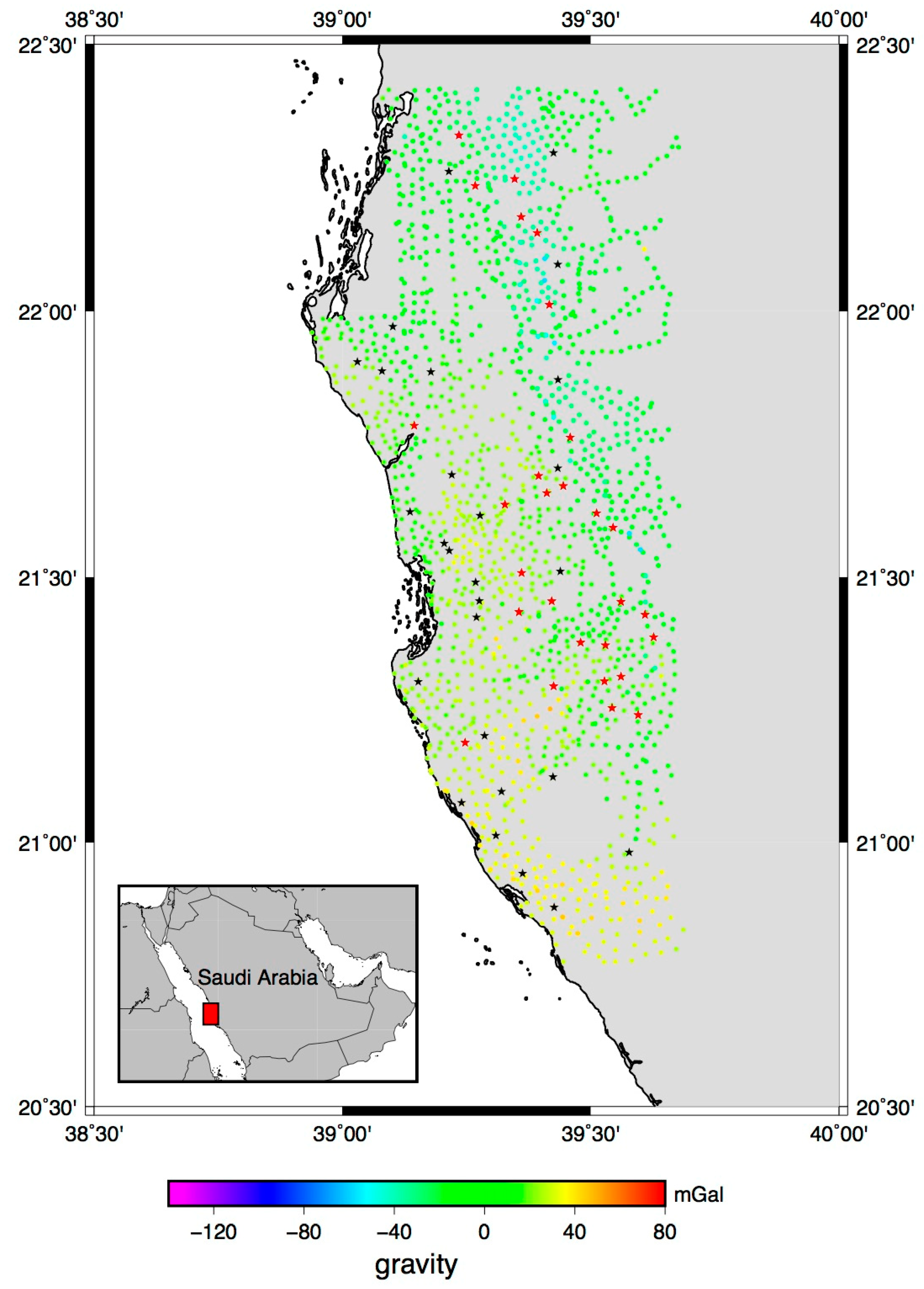
Following this procedure, 55 gravity values (3.3%) were selected as possible outliers, but only 21 of them were confirmed as such (1.2% of the total data set, with maximum and minimum difference values of 110.796 mgal and −32.590 mgal, respectively). In Figure 1, free-air gravity anomaly values are plotted in a color scale. The black stars are the suspected outliers pointed out by the 2σ rule, whereas the red ones are the outliers confirmed by Student’s t-inference test.
The new terrestrial gravity dataset was then combined by the sea gravity data provided by Bureau Gravimétrique International (BGI) [21] to improve the spatial coverage of the data and reduce the edge effects, and thus the gravity free-air database was formed with 4411 points.
3.3. The Global Geopotential Model
Nowadays, different Global Geopotential Models (GGM) are available thanks to the new satellite gravity missions, especially the Gravity Recovery and Climate Experiment (GRACE) [3,4] and the Gravity Field and Steady-State Ocean Circulation Explorer (GOCE) [2].
Different GGMs were taken into account and tested, looking for the one giving the best fit to the new terrestrial gravity dataset used in this study. Among the available GGMs investigated, satellite-only GGMs have also been considered, even if their maximum degree and order (300) in the spherical harmonic expansion is significantly lower than the one of combined GGMs (satellite and terrestrial combined solutions) that are complete to a higher degree and order (d/o) (e.g., 2190).
This has been done in order to check how effective new satellite-only GGMs, based on the GRACE and GOCE satellite missions, are in representing the low-frequency components of the gravity field, while also comparing them to the high-degree GGMs that are based on the combination of satellite and ground data. What we wanted to investigate with this comparison is the effectiveness of the high-degree GGMs in areas where only a small amount of terrestrial data were available, as is the case for the Arabic Peninsula. As is well known, in the EGM2008 computation [20], the 5 arc minute area mean gravity anomalies used for this geographic area are labelled as “fill-in” data. This means that, for this region, the 5 arc minute gravity anomalies were derived by 15 arc minute area mean value classified data. Thus, in this region, the quality of the data is quite poor. Furthermore, these “fill-in” data are also present in the other high-degree GGMs since they have been estimated using the same terrestrial database of EGM2008.
In this paper, GGMs labelled as timewise (GO_TIM), direct (GO_DIR) and spacewise (GO_SPW) are the satellite-only GGMs that have been considered [2]. The R4, R5 and R6 labels indicate the release of the GOCE-based GGMs. For instance, the R5 and R6 releases use GOCE data, spanning the complete mission lifetime, including the low-orbit data collected in the re-entry phase of the satellite in November 2013. The three solutions (GO_TIM, GO_DIR and GO_SPW) differ for the processing strategies of the same GOCE observations. GO_TIM and GO_DIR are based on the so-called timewise (GO_TIM) and direct (GO_DIR) approaches, respectively, whereas the latter is based on the so-called spacewise (GO_SPW) method [2]. The R6 release in each processing strategy (direct, timewise and spacewise) differs from the R5 release for an improved re-calibration of the GOCE satellite gradiometer components [22].
In Table 2, the global potential models are tested and their main characteristics are reported. The models highlighted in a grey color are the ones already tested and used in the 2014 geoid undulation estimate, whereas the others are the most recent models used in the new validation procedure for the geoid estimate.
3.4. Digital Terrain Model
The availability of a detailed Digital Terrain Model (DTM) is a key point in the computation of the residual terrain correction. Although a high resolution DTM (5 m × 5 m) is available for the Jeddah Municipality, the 3″ × 3″ DTM from the Shuttle Radar Topography Mission (SRTM3 [28] was preferred, because the gravity measurements are affected by the signal of the topography in an area larger than the computation area. Thus, a digital terrain model in an area wider than the one containing the gravity data is needed. For this reason, a homogeneous terrain model was preferred with respect to the highest resolution Jeddah DTM, which was available only over the Jeddah Municipality region.
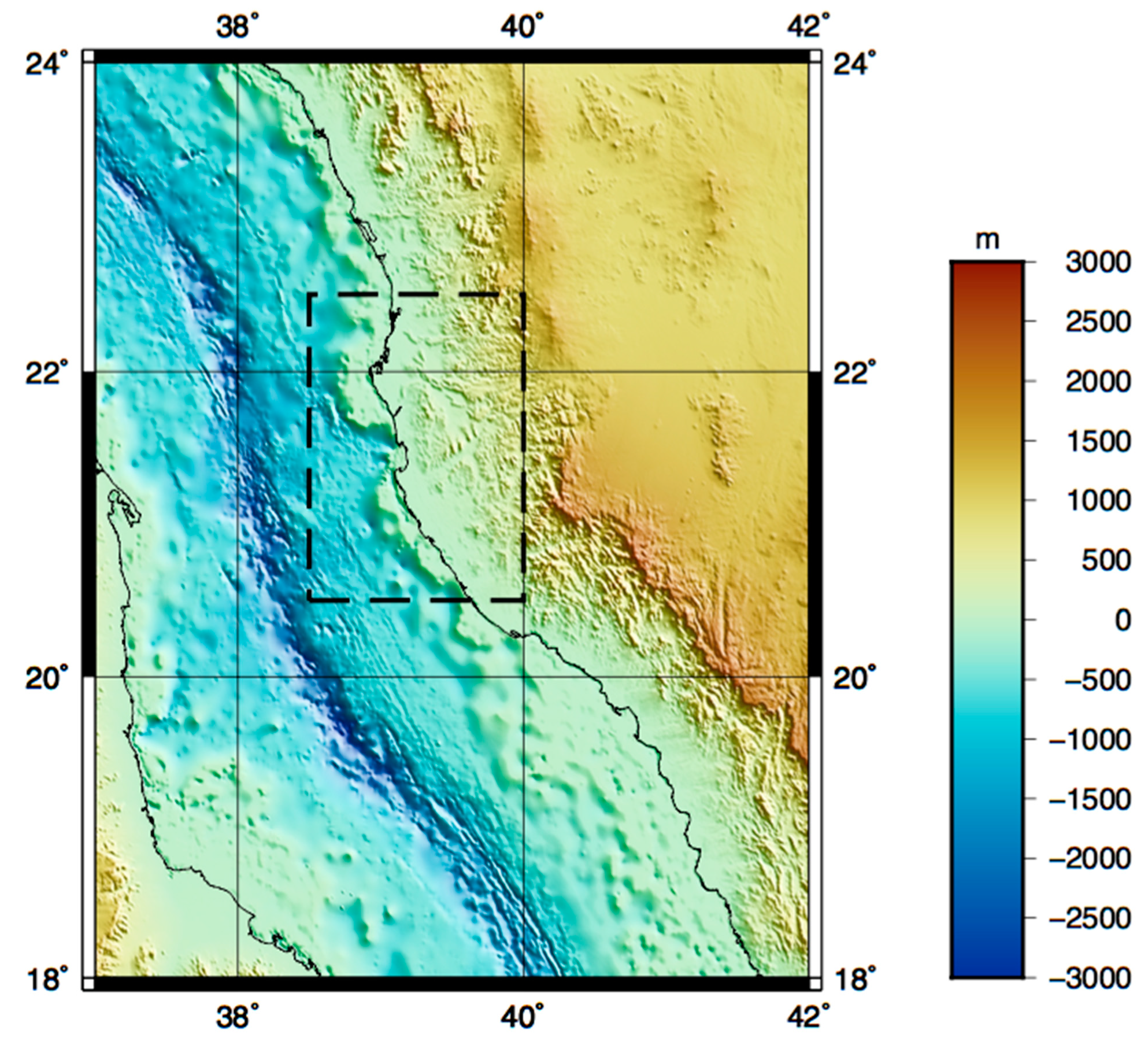
As the computation zone includes a portion of the Red Sea, the DTM model must be integrated with a bathymetric model. To this end, the bathymetric General Bathymetric Chart of the Oceans (GEBCO, [29]) grid has been merged with the SRTM3 model. The GEBCO grid has been interpolated by means of a bilinear interpolation to have the same resolution as the SRTM3 grid. Furthermore, the GEBCO grid, with a resolution of 30″ × 30″, has also data on land. These values have been used to fill the gaps in the SRTM3 grid. Figure 2 illustrates the assembled detailed DTM.
As is well known, Residual Terrain Correction (RTC) consists of the computation of the gravimetric effect of the terrain bounded by two surfaces. We computed this effect using the TC software of the GRAVSOFT package [11], selecting the standard density values 2670 kg m−3 and 1030 kg m−3 for the land and for the water, respectively. The first surface is the topographic surface, represented by the detailed DTM in Figure 2. The reference DTM is smoother than the first ones and should be correlated to the topography effect that is already taken into account by the used GGM (see Table 2). This surface is not known a priori and it depends on the maximum degree of the spherical harmonic expansion of the applied GGM. This smoother surface can be statistically identified by testing different smoothed versions of the available detailed DTM, computed by a moving average procedure based on different window sizes (in this work, from 5’ to 50’). The statistics of the residual gravity anomalies (Δgres) are then used in the choice of the best window size for the DTM averaging procedure. The smoothed reference DTM that gives the lowest values of the mean and standard deviation of the residual gravity anomalies is the proper reference DTM to be considered in the RTC computation. As the average DTM is correlated to the geopotential model used to compute the residuals, for each considered GGM, an analysis of the size of the averaging window has been performed. By using this approach, we optimized both the d/o of each considered GGM and the reference DTM to be used in the RCR procedure (Table 2).
4. Result and Discussion
4.1. The Remove–Compute–Restore Results
In the remove step of the RCR procedure, gravity data are reduced for the low- and high- frequency components. In Table 3, the statistics of the remove step are given for each used GGM. For each solution based on different GGMs, the statistics of the ∆gres show the different features of the gravity residuals in relation to the d/o of the used GGM. This can also be seen in the structure of the empirical auto-covariance functions that are described herein.
The prediction on a 1′ × 1′ mesh grid of the residual height anomaly estimation ζres was performed using the least squares collocation (LSC) method ([13,14]). The LSC method is based on the estimate of the empirical auto-covariance function (ACF) of the residual gravity anomalies and its interpolation with a positive definite function, called the covariance function model ([30,31,32]).
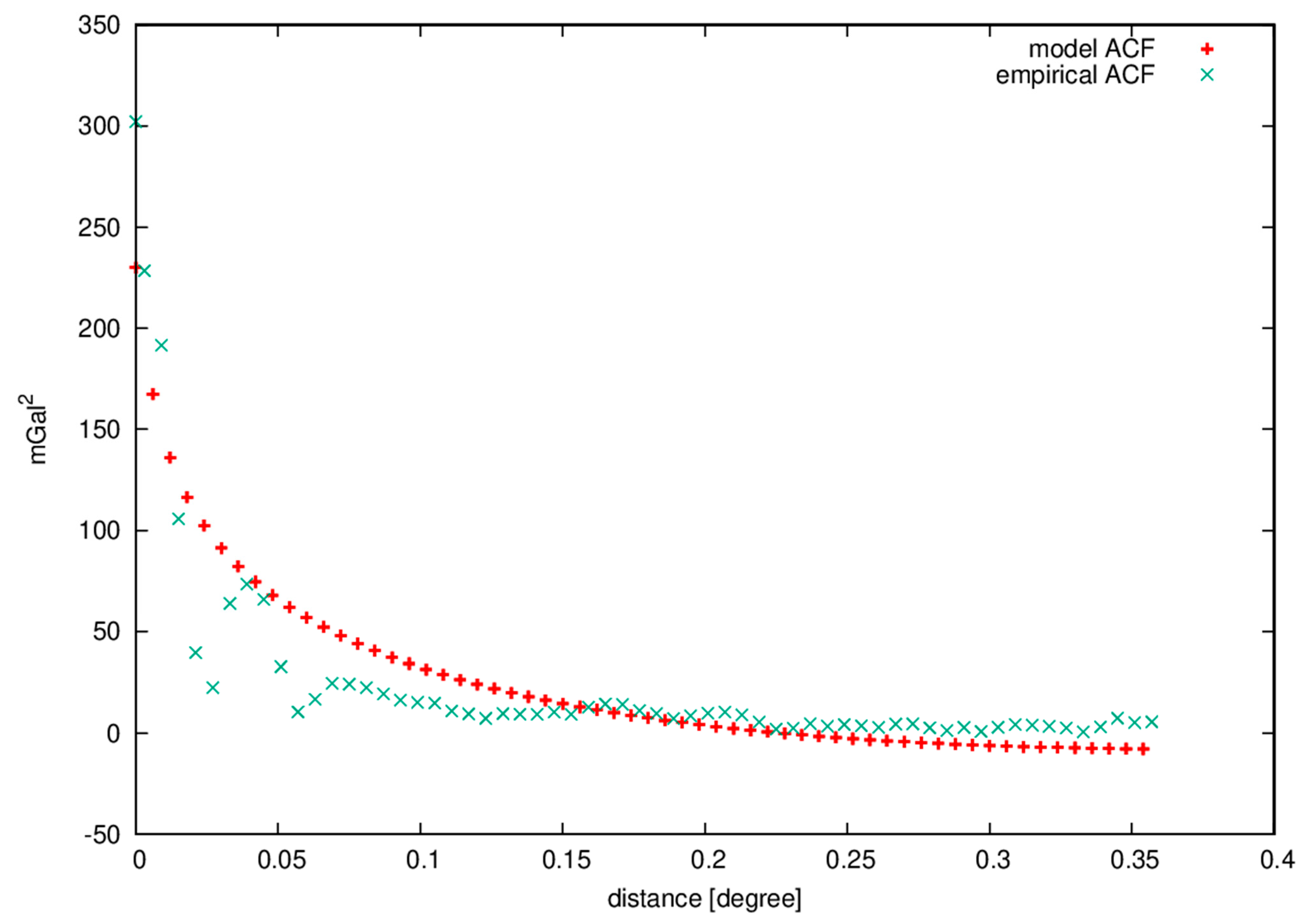
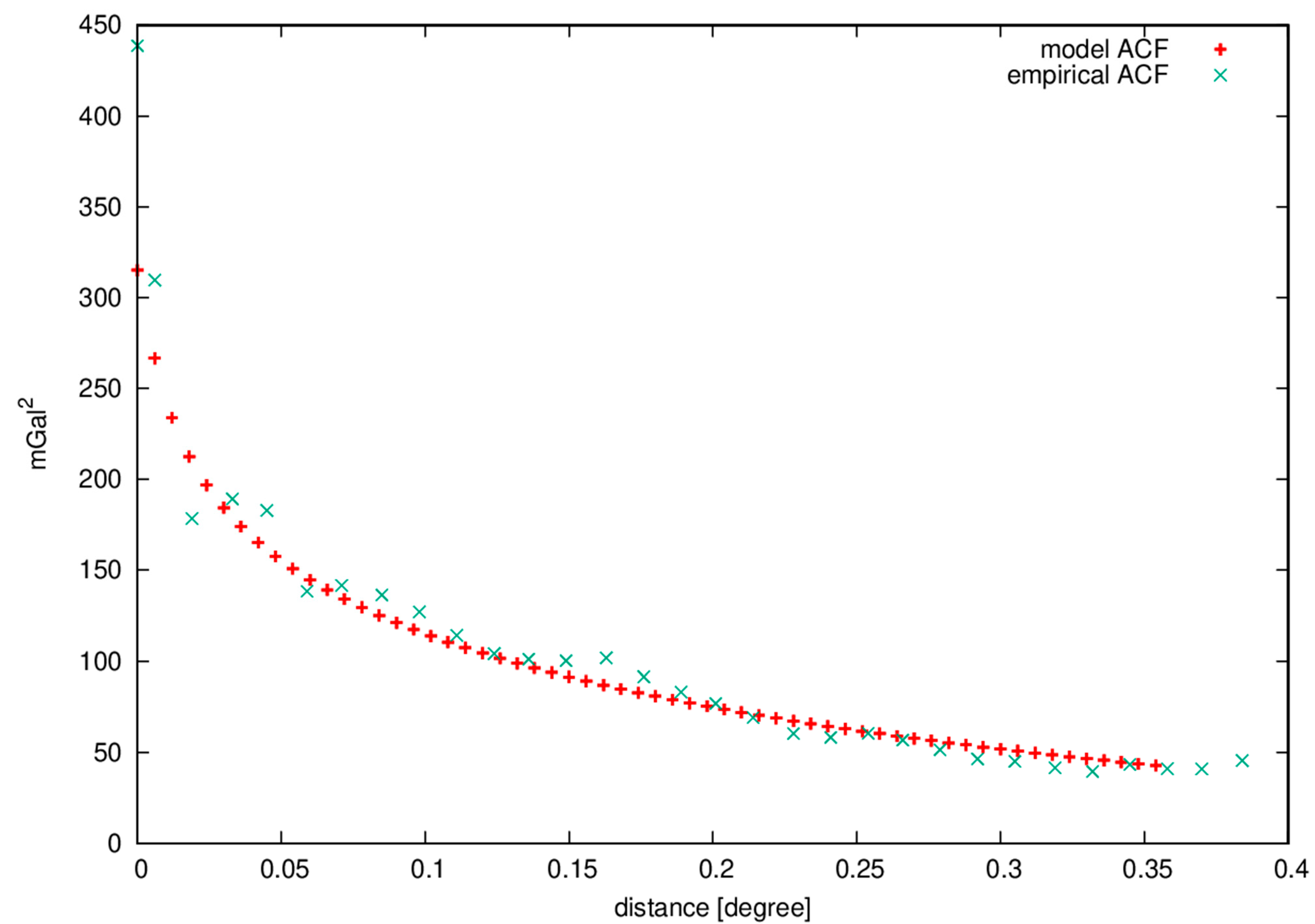
The magnitude of the variance of the signal and the correlation length of the ACFs are different, due to different GGMs and RTC computations used in the remove step. In Figure 3 and Figure 4, empirical auto-covariance functions and best-fit covariance models for the reduced values obtained with EGM2008 and GO_DIR_R5 are plotted, respectively. As expected, the residual free-air gravity anomalies obtained with GO_DIR_R5 have a longer correlation length than the corresponding ones obtained using a higher order degree model, i.e., EGM2008, even though the difference in the correlation length is not as sharp.
The magnitude of the residual signals ζres (Table 4), estimated by LSC, also reflects the different behaviors based on the adopted GGM. The solutions based on the low d/o GGMs (up to 250) have height anomaly values that can reach 1 m with a mean value of about 30 cm or more. On the contrary, the height anomaly values ζres estimated from the high-resolution GGMs (d/o 1800) have mean values of about 8 cm and maximum and minimum values smaller than 25 cm in absolute value. The solutions based on GOCO05c and XGM2016 have intermediate statistics with respect to the ones described above.
The Compute step of the RCR procedure was then followed by the restore step. The long-wavelength components (GGM) coming from the different GGMs considered in this study and the topographic short-wavelength components (RTC) of the height anomaly were then computed and added to the residual height anomaly (), obtained by LSC.
4.2. Validation of the Gravimetric Geoid Model
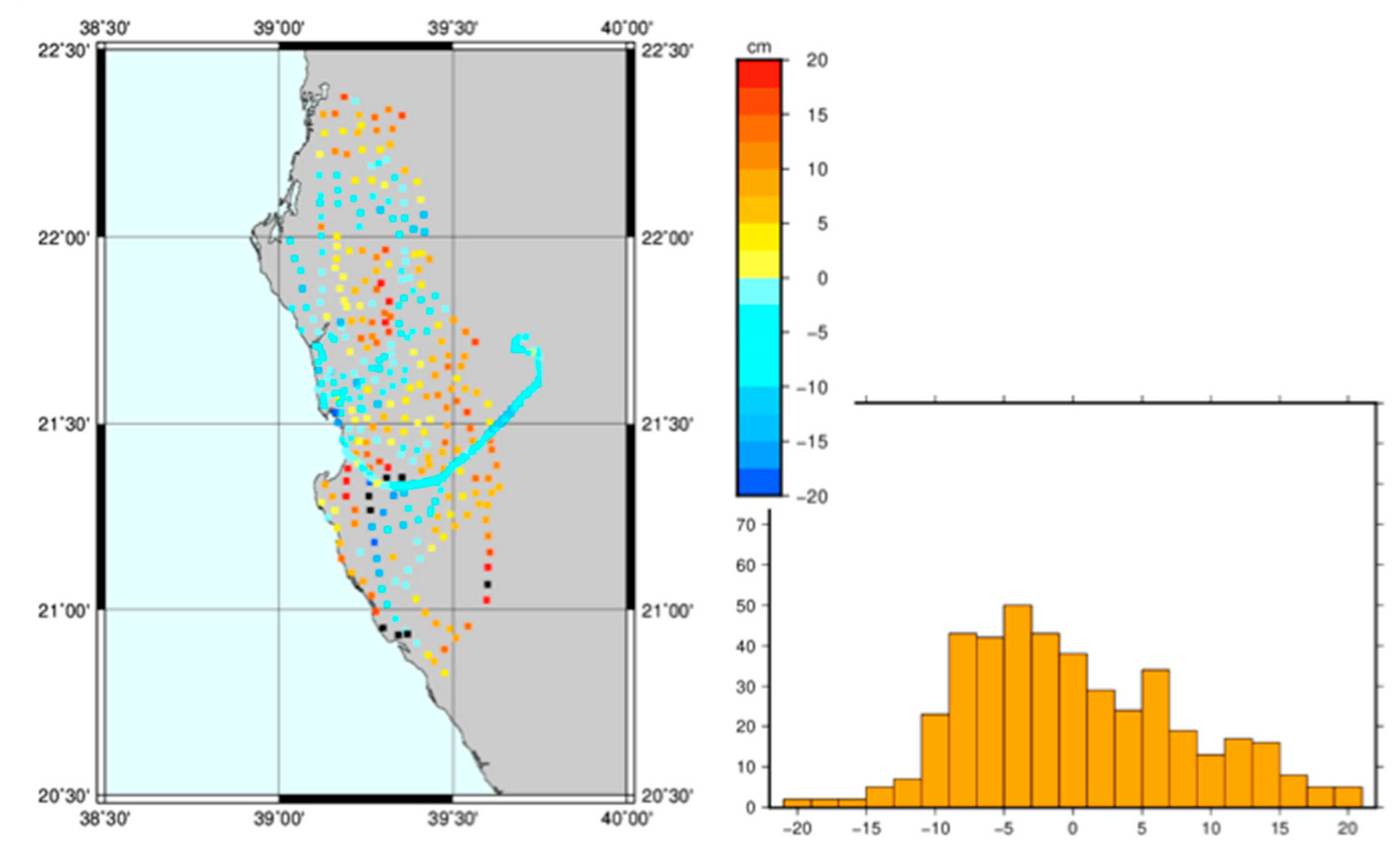
The precision of the estimated gravimetric geoid models has been assessed by comparing their geoid undulation values with those obtained by GPS/levelling observations collected in the framework of this project for a set of points distributed in the investigated area (see Figure 5).
As we have adopted the Molodensky theory, the estimated height anomalies have to be transformed in geoid undulations using Equation (2) to be coherently compared with the geoid undulations obtained by the orthometric H and the GPS ellipsoidal heights hGPS, that is NGPS/lev = hGPS –H. In Table 5, statistics of the differences between the gravimetric geoid undulations and NGPS/lev are reported. Independently of the GGM used, the differences present significant discrepancies. This is mainly due to the different reference systems in which the gravimetric and the GPS/levelling-derived geoid undulations are given. Thus, in order to enable a proper comparison, a datum transformation must be estimated. According to Section 2 [33], a three-parameter transformation (dx, dy, dz) using formula (5) can be used:
where θ is the co-latitude, that is θ = 90° − ϕ, and λ ϕ are the longitude and the latitude of the computation point.
Ngrav = NGPS/lev + ΔN(θ,λ) = NGPS/lev + dx sinθ cosλ+ dy sinθ sinλ + dz cosθ
The statistics of the least squares differences represent an estimate of the precision of the gravimetric geoid undulation (Table 6). An outlier rejection is also performed on the least squares differences of the datum transformation, under the hypothesis of normally distributed values at a significance level of 1%. As can be observed, the number of points reported in Table 5 is different from one solution to another since different geoid solutions were used and the outlier rejection gave us different results.
As the standard deviation of the differences is about 7.5–8.0 cm, the geoid estimates obtained using the satellite-only GGMs and the XGM2016 GGM are those that are in better agreement with the GPS/levelling geoid undulation values with respect the model based on the other GGMs. These statistics confirm our hypothesis about the reliability of the satellite-only GGMs in areas poorly covered by terrestrial gravity data and show the important contribution of the GOCE mission.
4.3. The Hybrid Estimate of the Height Anomaly and Geoid Undulation
The availability of a dense set of GPS/levelling points—that is, points with known orthometric and ellipsoidal heights, allows for the estimation of a hybrid geoid model for the Jeddah Municipality ([9,10]). The gravimetric observations and the height anomalies coming from the difference in the GPS and spirit levelling observations can be integrated together, again, by using the LSC estimator.
The integration procedure is based on a revised “Remove–Compute–Restore” approach: the residual gravity anomalies (Δgres) are integrated into the LSC procedure with the residual GPS/levelling height anomalies (GPS/lev_res obtained by GPS/levelling geoid undulations and applying formula (2)), found by subtracting the long-wavelength component (GGM), using a global geopotential model and the topographic short-wavelength component (RTC). In the LSC estimator, the vector of the observations is now given by ) and the covariance matrix C is a block matrix, composed of the gravity covariance matrix CΔgΔg, the covariance matrix Cζζ of the height anomalies and the cross-covariance matrix CζΔg. The covariance matrix of the gravity data is the same used in the pure gravimetric solution (Figure 1), whereas the covariance matrix Cζζ and the cross-covariance CζΔg are obtained via covariance propagation from CΔgΔg. On the main diagonal of the Cζζ matrix, the height anomaly variance is added. This value is chosen by assuming that the standard deviation of the height anomalies obtained from GPS/levelling data is about 3 cm, which represents a realistic value, taking into account the precision in the GPS and the levelling observations given in Section 3.
The result of the LSC computation is the set of hybrid residual height anomalies , as shown in Equation (5), to which the long-wavelength term (GGM) and the topographic high-frequency component (RTC) will be added in order to complete the restore step.
As we have presented in the previous section, the available GPS/levelling data set consisted of 443 points. Some of these values have been detected as outliers in the validation procedure of the pure gravimetric geoid model, so these points have been removed from the data set considered in the hybrid estimate. In the hybrid geoid estimate, only the values in the range from −10 to 10 cm, with respect to the pure gravimetric geoid undulations, have been taken into account. These values, about 80% of the total database, are selected according a 3σ criterion, based on the precision of the GPS-derived heights (see Section 3). Furthermore, this reduced data set was randomly divided into two subsets, A and B, where about the 2/3 of the entire dataset is in set A. Set A was integrated with the gravimetric observations to obtain the hybrid quasigeoid model, whereas set B was used as an independent dataset to validate the results.
At the end of this estimate, the height anomaly values were converted into geoid undulation, according to the approximate formula of Equation (2).
4.4. Validation of the Hybrid Geoid Model
The first validation of the data was performed on set A of the GPS/levelling geoid undulations. This is only a consistency control to check whether the relative weights between gravity and geoid undulation data are correctly set up. In Table 7, the statistics of the differences between the hybrid geoid models and GPS/levelling geoid undulations, after the datum shift reduction, are reported.
The second independent validation was then done for set B. The hybrid geoid model was interpolated onto the points in set B with a bilinear interpolation and the differences between the GPS/levelling geoid undulations were computed (statistics in Table 7).
The integration procedure has significantly improved the precision of the geoid estimate in the Jeddah Municipality. The standard deviations of the best pure gravimetric solutions are of the order of 7.5–7.8 cm, while the standard deviation of the hybrid solution decreases to 3.7 cm. The different hybrid solutions obtained by using different satellite-only GGMs have similar statistics, better than the ones of the combined GGMs, such as EGM2008, EIGEN-6c2, EIGEN-6c4 and GOCO05c. Furthermore, the recent XGM2016 model gives results of the same order of precision of the solutions based on the satellite-only GGMs.
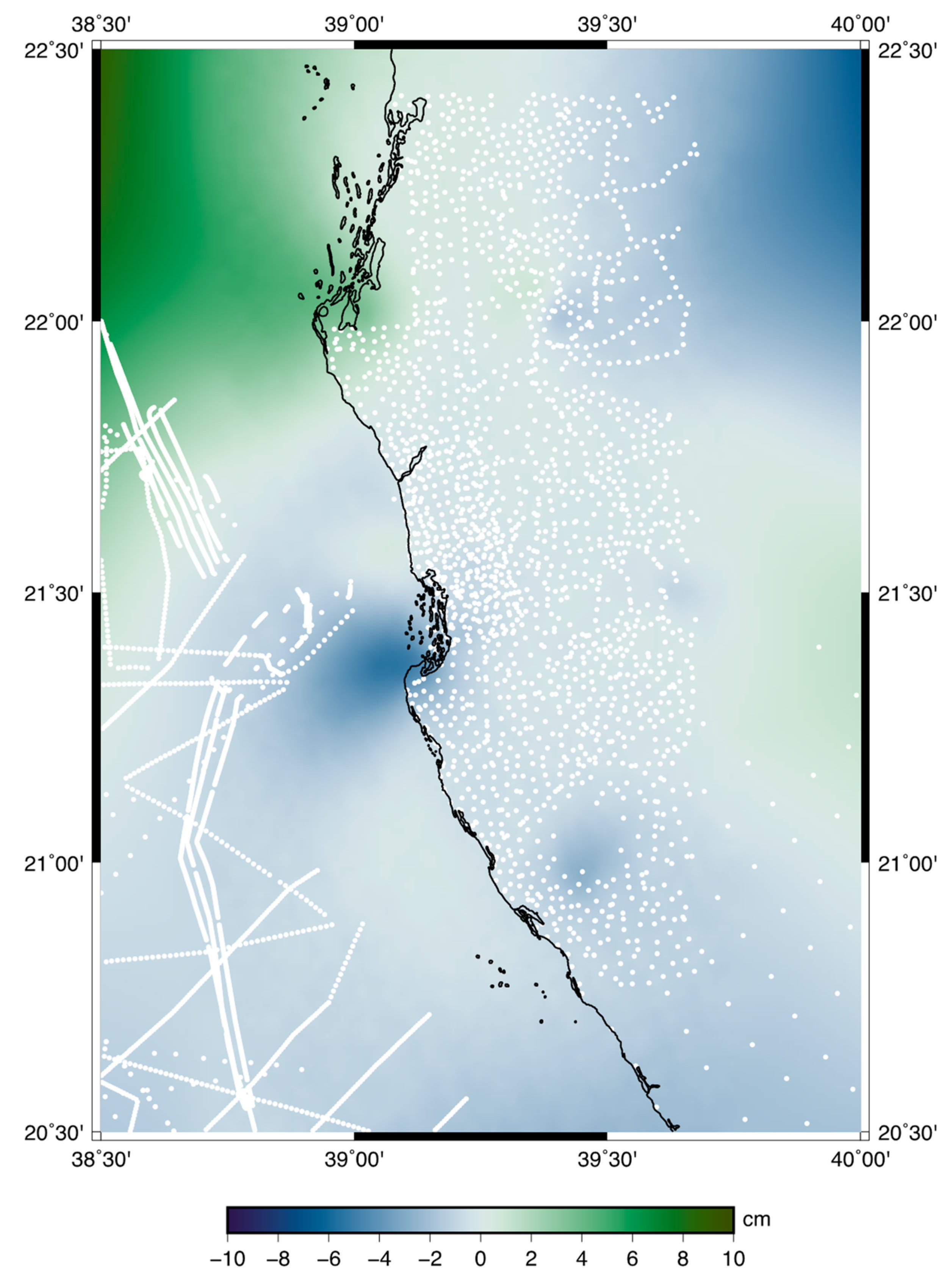
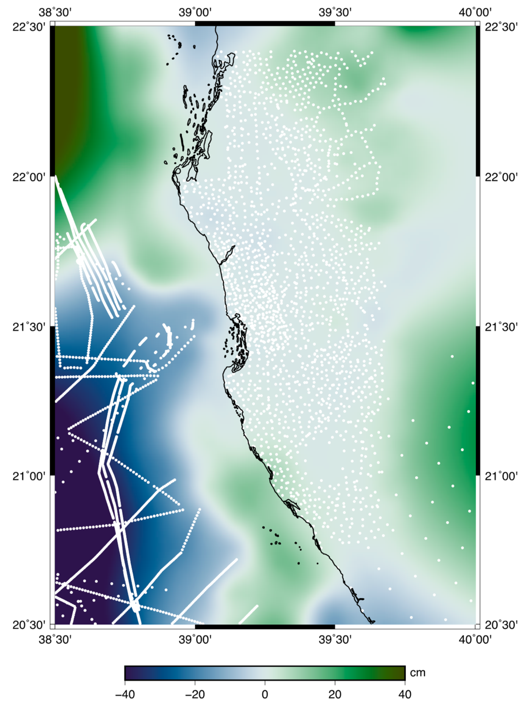
The comparison of different geoid undulation solutions shows good agreement in the area covered by terrestrial gravity data and GPS/levelling points, as shown in Figure 6, where the differences between the hybrid geoid model determined by the solution GO_SPW_R5 and the ones developed by the solution GO_DIR_R5 are reported. Outside the area covered by ground data, the differences are larger, in the range from −10 to 10 cm when we compare solutions based on satellite-only models. On the other hand, when comparing, for instance, the solution based on GO_SPW_R5 and the solution based on XGM2016, one has higher differences in the sea, even where gravity data are present (Figure 7). This behavior seems to prove that, between the two geoid models, there is a tilt effect that has been mitigated only in the central part of the computation area where the GPS/levelling data were collected.
5. Conclusions
In 2014, the Jeddah Municipality made a call for an estimate of a centimetric precision geoid model to be used for engineering and surveying applications. A project was set up to this end and dedicated sets of gravity and GPS/levelling data were acquired in the framework of this project. In this paper, a thorough analysis of these newly acquired data, of the DTM and of the available GGMs has been exploited in order to obtain a geoid undulation estimate with the prescribed precision. In the framework of the RCR approach, the least squares collocation method was used to estimate the height anomaly estimation, which was then converted to geoid undulation. This procedure has been applied based on different GGMs with different d/o resolutions. Furthermore, two different quasi-geoid collocation estimates were computed, based on gravity data only and on gravity plus GPS/levelling data (the so-called hybrid estimate). The best solutions were obtained in the hybrid geoid estimate. This was tested by comparison with an independent set of GPS/levelling geoid undulations that were not included in the computed solutions. Through these tests, the precision of the hybrid geoid, i.e., 3.7 cm, proved to be better, by a factor of two, compared to the precision of the pure gravimetric geoid, i.e., 7.5 cm.
As a byproduct, the estimate of the geoid undulation for the Jeddah Municipality using the newly collected data also gave us the opportunity to test the newly developed GGMs, estimated with the data from the GRACE and the GOCE satellite gravity missions.
All the solutions based on satellite-only GGMs had higher precision in terms of the geoid undulation estimate. Moreover, the old releases of the satellite-only GGMs, as well as the R4 release of the GO_DIR approach, show a good performance, somehow even better than the newer solutions. Thus, for this reason, the geoid undulation model computed in 2014 for the Jeddah Municipality can be still considered reliable.
Finally, it must be remarked that the new XGM2016 GGM is also a promising model in view of the computation of the new generation of combined GGMs. In fact this model can be considered the precursor step for the combined Earth Gravitational Model 2020 (EGM2020).
Through the definition of the Jeddah2014 Vertical Reference Frame, different research groups have improved and validated geoid undulation models all over the Kingdom of Saudi Arabia (KSA), i.e., KSA-GEOID17 and SAGE013 [34,35,36], so we believe that this work, although focused on a small region of the KSA, could give important information about the GGMs that can be used and about their expected precision.
Author Contributions
Conceptualization, A.B., R.B. and O.A.-B.; methodology, A.B and R.B.; software, A.B. and R.B.; validation, A.B and R.B.; resources, O.A.-B. and S.A.M.; writing—original draft preparation, A.B.; writing—review and editing, A.B. and R.B.; project administration, O.A.-B. and S.A.M.; funding acquisition, S.A.M. All authors have read and agreed to the published version of the manuscript.
Funding
This research received no external funding.
Conflicts of Interest
The authors declare no conflict of interest.
References
- Alothman, A.; Bouman, J.; Gruber, T.; Lieb, V.; Alsubael, M.; Alomar, A.; Fuchs, M.; Schmidt, M. Validation of Regional Geoid Models for Saudi Arabia Using GPS/Levelling Data and GOCE Models. In Gravity, Geoid and Height Systems; Marti, U., Ed.; Springer: Cham, Switzerland, 2014; Volume 141, pp. 193–199. [Google Scholar] [CrossRef]
- Pail, R.; Bruinsma, S.L.; Migliaccio, F.; Förste, C.; Goiginger, H.; Schuh, W.D.; Höck, E.; Reguzzoni, M.; Brockmann, J.M.; Abrikosov, O.; et al. First GOCE gravity field models derived by three different approaches. J. Geod. 2011, 85, 819–843. [Google Scholar] [CrossRef] [Green Version]
- Tapley, B.D.; Bettadpur, S.; Ries, J.C.; Thompson, P.F.; Watkins, M.M. GRACE measurements of mass variability in the earth system. Science 2004, 305, 503–505. [Google Scholar] [CrossRef] [PubMed] [Green Version]
- Tapley, B.D.; Bettadpur, S.; Watkins, M.; Reigber, C. The gravity recovery and climate experiment: Mission overview and early results. Geophys. Res. Lett. 2004, 31, L09607. [Google Scholar] [CrossRef] [Green Version]
- Ince, E.S.; Barthelmes, F.; Reißland, S.; Elger, K.; Förste, C.; Flechtner, F.; Schuh, H. ICGEM–15 years of successful collection and distribution of global gravitational models, associated services, and future plans. Earth Syst. Sci. Data 2019, 11, 647–674. [Google Scholar] [CrossRef] [Green Version]
- Förste, C.; Bruinsma, S.L.; Abrikosov, O.; Lemoine, J.M.; Marty, J.C.; Flechtner, F.; Balmino, G.; Barthelmes, F.; Biancale, R. EIGEN-6C4 the latest combined global gravity field model including GOCE data up to degree and order 2190 of GFZ Potsdam and GRGS Toulouse. GFZ Data Serv. 2014. [Google Scholar] [CrossRef]
- Fecher, T.; Pail, R.; Gruber, T. Global gravity field modeling based on GOCE and complementary gravity data. Int. J. Appl. Earth Obs. Geoinf. 2015, 35, 120–127. [Google Scholar] [CrossRef]
- Pail, R.; Fecher, T.; Barnes, D.; Factor, J.F.; Holmes, S.A.; Gruber, T.; Zingerle, P. Short note: The experimental geopotential model XGM2016. J. Geod. 2018, 92, 443–451. [Google Scholar] [CrossRef]
- Albertella, A.; Barzaghi, R.; Carrion, D.; Maggi, A. The joint use of gravity data and GPS/levelling undulations in geoid estimation procedures. Bollettino di Geodesia e Scienze Affini 2008, 1, 47–57. [Google Scholar]
- Chen, Y.-Q.; Luo, Z. A hybrid method to determine a local geoid model-Case study. Earth Planets Space 2004, 56, 419–427. [Google Scholar] [CrossRef] [Green Version]
- Forsberg, R.; Tscherning, C.C. An. overview Manual for the GRAVSOFT Geodetic Gravity Field Modelling Programs, 2nd ed.; DTU Space: Kongens Lyngby, Denmark, 2008. [Google Scholar]
- Forsberg, R. A Study of Terrain Corrections, Density Anomalies and Geophysical Inversion Methods in Gravity Field Modelling. In Reports of the Department of Geodesy Science and Survey; Ohio State University: Columbus, OH, USA, 1984; Volume 355. [Google Scholar]
- Moritz, H. Advanced Physical Geodesy, 2nd ed.; Wichmann: Karlsruhe, Germany, 1980. [Google Scholar]
- Krarup, T. Mathematical Foundations of Geodesy; Borre, K., Ed.; Springer: Berlin, Germany, 2006. [Google Scholar]
- Sansò, F.; Sideris, M. Geoid Determination. In Theory and Methods; Springer Verlag GmbH: Heidelberg, Germany, 2013; ISBN 978-3-540-74699-7. [Google Scholar] [CrossRef]
- Hofmann-Wellenhof, B.; Moritz, H. Physical Geodesy; Springer Wien: NewYork, NY, USA, 2006. [Google Scholar]
- Flury, J.; Rummel, R. On the geoid–quasigeoid separation in mountain areas. J. Geod. 2009, 83, 829–847. [Google Scholar] [CrossRef]
- Moritz, H. Geodetic reference system. Bulletin Géodésique 1980, 54, 395–405. [Google Scholar] [CrossRef]
- Barzaghi, R.; Borghi, A.; Carrion, D.; Sona, G. Refining the estimate of the Italian quasi-geoid. Bollettino di Geodesia e Scienze Affini 2007, 3, 145–160. [Google Scholar]
- Pavlis, N.K.; Holmes, S.A.; Kenyon, S.C.; Factor, J.K. The development and evaluation of the Earth Gravitational Model 2008 (EGM2008). J. Geophys. Res. Solid Earth 2012, 117, B04406. [Google Scholar] [CrossRef] [Green Version]
- Bureau Gravimetrique International (BGI). Available online: http://bgi.omp.obs-mip.fr/data-products/terms_of_use (accessed on 24 June 2020). [CrossRef]
- Siemes, C.; Rexer, M.; Schlicht, A.; Haagmans, R. GOCE gradiometer data calibration. J. Geod. 2019, 93, 1603–1630. [Google Scholar] [CrossRef]
- Gatti, A.; Reguzzoni, M. GOCE gravity field model by means of the space-wise approach (release R5). GFZ Data Serv. 2017. [Google Scholar] [CrossRef]
- Bruinsma, S.L.; Forste, C.; Abrikosov, O.; Marty, J.-C.; Rio, M.-H.; Mulet, S.; Bonhlot, S. The new ESA satellite-only gravity field model via the direct approach. GRL 2014, 40, 3607–3612. [Google Scholar] [CrossRef] [Green Version]
- Förste, C.; Abrykosov, O.; Bruinsma, S.; Dahle, C.; König, R.; Lemoine, J.-M. ESA’s Release 6 GOCE gravity field model by means of the direct approach based on improved filtering of the reprocessed gradients of the entire mission (GO_CONS_GCF_2_DIR_R6). GFZ Data Serv. 2019. [Google Scholar] [CrossRef]
- Brockmann, J.M.; Schubert, T.; Mayer-Gürr, T.; Schuh, W.-D. The Earth’s gravity field as seen by the GOCE satellite—An improved sixth release derived with the time-wise approach (GO_CONS_GCF_2_TIM_R6). GFZ Data Serv. 2019. [Google Scholar] [CrossRef]
- Zingerle, P.; Brockmann, J.M.; Pail, R.; Gruber, T.; Willberg, M. The polar extended gravity field model TIM_R6e. GFZ Data Serv. 2019. [Google Scholar] [CrossRef]
- Farr, T.G.; Rosen, P.A.; Caro, E.; Crippen, R.; Duren, R.; Hensley, S.; Kobrick, M.; Paller, M.; Rodriguez, E.; Roth, L.; et al. The Shuttle Radar Topography Mission. Rev. Geophys. 2007, 45, RG2004. [Google Scholar] [CrossRef] [Green Version]
- GEBCO Bathymetric Compilation Group. The GEBCO_2019 Grid—A Continuous Terrain Model of the Global Oceans and Land; British Oceanographic Data Centre, National Oceanography Centre, NERC: Liverpool, UK, 2019. [Google Scholar]
- Tscherning, C.C.; Rapp, R.H. Closed Covariance Expressions for Gravity Anomalies, Geoid Undulations, and Deflections of the Vertical Implied by Anomaly Degree Variances; Rep No 208, Department of Geodetic Sciences and Surveying; The Ohio State University: Columbus, OH, USA, 1974. [Google Scholar]
- Tscherning, C.C. Covariance Expressions for Second and Lower Order Derivatives of the Anomalous Potential; Reports of the Department of Geodesy Science and Survey; Ohio State University: Columbus, OH, USA, 1976; Volume 225. [Google Scholar]
- Knudsen, P. Estimation and modelling of the local empirical covariance function using gravity and satellite altimeter data. Bull. Geod 1987, 61, 145–160. [Google Scholar] [CrossRef]
- Heiskanen, W.A.; Moritz, H. Physical Geodesy, Institute of Physical Geodesy; Technical University of Graz: Graz, Austria, 1990. [Google Scholar]
- Abdalla, A.; Mogren, S. Implementation of a rigorous least-squares modification of Stokes’ formula to compute a gravimetric geoid model over Saudi Arabia (SAGEO13). Can. J. Earth Sci. 2015, 52, 823–832. [Google Scholar] [CrossRef] [Green Version]
- Elsaka, B.; Alothman, A.; Godah, W. On the Contribution of GOCE Satellite-Based GGMs to Improve GNSS/Leveling Geoid Heights Determination in Saudi Arabia. IEEE J. Sel. Topics in Appl. Earth Obs. Remote Sens. 2016, 9, 5842–5850. [Google Scholar] [CrossRef]
- Alothman, A.; Godah, W.; Elsaka, B. Gravity field anomalies from recent GOCE satellite-based geopotential models and terrestrial gravity data: A comparative study over Saudi Arabia. Arab. J. Geosci. 2016, 9, 356. [Google Scholar] [CrossRef]
Figure 1.
Free-air gravity anomalies of the new measured database in the Jeddah Region of Saudi Arabia (red rectangle in the bottom left box). The black stars represent the suspected outliers; the red stars represent the confirmed outliers.
Figure 1.
Free-air gravity anomalies of the new measured database in the Jeddah Region of Saudi Arabia (red rectangle in the bottom left box). The black stars represent the suspected outliers; the red stars represent the confirmed outliers.

Figure 2.
Assembled 3″ × 3″ grid of DTM for the Residual Terrain Correction computation, obtained by merging the SRTM3 3″ × 3″ and General Bathymetric Chart of the Oceans (GEBCO) 30″ × 30″ grids. The dashed black box represents the computation area.
Figure 2.
Assembled 3″ × 3″ grid of DTM for the Residual Terrain Correction computation, obtained by merging the SRTM3 3″ × 3″ and General Bathymetric Chart of the Oceans (GEBCO) 30″ × 30″ grids. The dashed black box represents the computation area.

Figure 3.
Empirical (green crosses) and model (red symbols) [30,31] of the auto-covariance functions reducing the residual gravity observations for the Earth Gravitational Model 2008 (EGM2008) up to degree 1800 (see Table 2). Auto-covariance function (ACF).

Figure 4.
Empirical (green crosses) and model (red symbols) [30,31] of the auto-covariance functions reducing the residual gravity observations timewise (GO_TIM)_R5 up to degree 240.

Figure 5.
The spatial distribution and histogram of the differences between gravimetric undulations and the GPS/levelling values after datum shift estimate (values in centimeters). This represents the solution based on the spacewise (GO_SPW)_R5 GGM.
Figure 5.
The spatial distribution and histogram of the differences between gravimetric undulations and the GPS/levelling values after datum shift estimate (values in centimeters). This represents the solution based on the spacewise (GO_SPW)_R5 GGM.

Figure 6.
Differences between the geoid undulations derived by the hybrid models, based on GO_SPW_R5 and direct (GO_DIR)_R5 GGMs. The white dots represent the whole gravity database used.
Figure 6.
Differences between the geoid undulations derived by the hybrid models, based on GO_SPW_R5 and direct (GO_DIR)_R5 GGMs. The white dots represent the whole gravity database used.

Figure 7.
Differences between the geoid undulations derived by the hybrid models, based on GO_SPW_R5 and GO_XGM2016 GGM. The white dots represent the whole gravity database used.
Figure 7.
Differences between the geoid undulations derived by the hybrid models, based on GO_SPW_R5 and GO_XGM2016 GGM. The white dots represent the whole gravity database used.


Table 1.
Scheme of the Remove–Compute–Restore (RCR) procedure for the estimate of the geoid undulation, using gravity anomalies Δg and the Molodensky theory. Free air (FA); derived by a Global Gravity Field Model (GGM); residual terrain correction (RTC); residual component (res). N is the geoid undulation; is the height anomaly.
| Remove step: | ΔgFA − ∆gGGM − ∆gRTC = ∆gres |
| Compute step: | res = Collocation(∆gres) |
| Restore step: | res + GGM + RTC = |
| Geoid undulation | N = + ΔgB H |
Table 2.
Maximum degree/order (d/o) harmonic coefficients of the Global Gravity Models (GGMs) used in the computation and tested in relations to the spherical window size of the moving average of the detailed Digital Terrain Model (DTM). For each GGM, the fourth and fifth columns represent the chosen combination parameters (d/o and window size), giving the best statistics for the gravity residuals. In the last column, S means satellite, A altimetry and T gravity terrestrial data. The spherical models highlighted in grey are GGMs already tested in 2014 when the project was set up.
| GGM | Maximum d/o Available | d/o Tested | d/o Used | Window Size for the DTM Averaging | Type of Data |
|---|---|---|---|---|---|
| EGM2008 [20] | 2190 | 360, 720, 1080, 1440, 1800, 2190 | 1800 | 5’ | S–A–T |
| EIGEN-6c2 [5] | 1949 | 360, 720, 1080, 1440, 1800, 2190 | 1800 | 5’ | S–A–T |
| EIGEN-6c4 [6] | 2190 | 360, 720, 1080, 1440, 1800, 2190 | 1800 | 5’ | S–A–T |
| GOCO05c [7] | 720 | 360, 720 | 360 | 35’ | S–A–T |
| GO_SPW_R4 [5] | 280 | 220, 230, 240, 250, 260, 270, 280 | 250 | 35’ | S |
| GO_SPW_R5 [23] | 330 | 220, 230, 240, 250, 260, 270, 280, 290, 300, 310, 320, 330 | 240 | 35’ | S |
| GO_DIR_R4 [24] | 260 | 220, 230, 240, 250, 260 | 240 | 35’ | S |
| GO_DIR_R5 [24] | 300 | 220, 230, 240, 250, 260, 270, 280, 290, 300 | 240 | 35’ | S |
| GO_DIR_R6 [25] | 300 | 240 (437.172) | 240 | 35’ | S |
| GO_TIM_R4 [2] | 250 | 220, 230, 240, 250 | 230 | 35’ | S |
| GO_TIM_R5 [24] | 280 | 220, 230, 240, 250, 260, 270, 280 | 240 | 35’ | S |
| GO_TIM_R6 [26] | 300 | 220, 230, 240, 250, 260, 270, 280, 290, 300 | 240 | 35’ | S |
| GO_TIM_R6e [27] | 300 | 220, 230, 240, 250, 260, 270, 280, 290, 300 | 240 | 35’ | S |
| XGM2016 [8] | 719 | 360, 719 | 719 | 15’ | S–A–T |
Table 3.
Statistics of gravity residuals of 4411 gravity points, at the end of the “remove” step: ∆gFA − ∆gGGM − ∆gRTC = ∆gres testing different GGMs. For reference, in the last row (all highlighted in grey) we report the statistic values of ∆gFA (mGal).
Table 3.
Statistics of gravity residuals of 4411 gravity points, at the end of the “remove” step: ∆gFA − ∆gGGM − ∆gRTC = ∆gres testing different GGMs. For reference, in the last row (all highlighted in grey) we report the statistic values of ∆gFA (mGal).
| ∆gres | Mean | St. dev. | Min. | Max. | Root Mean Square |
|---|---|---|---|---|---|
| EGM2008 | 0.584 | 17.382 | −61.409 | 61.480 | 17.40 |
| EIGEN-6c2 | 1.715 | 17.229 | −57.859 | 62.405 | 17.31 |
| EIGEN-6c4 | 1.821 | 17.304 | −59.210 | 63.032 | 17.40 |
| GOCO05c | 4.519 | 19.986 | −71.299 | 88.139 | 20.49 |
| GO_SPW_R4 | 2.327 | 20.735 | −69.548 | 80.374 | 20.87 |
| GO_SPW_R5 | 2.346 | 21.117 | −70.904 | 76.367 | 21.25 |
| GO_DIR_R4 | 2.004 | 21.300 | −70.776 | 79.684 | 21.39 |
| GO_DIR_R5 | 2.372 | 20.796 | −71.121 | 76.530 | 20.93 |
| GO_DIR_R6 | 2.156 | 20.797 | −72.120 | -74.056 | 20.91 |
| GO_TIM_R4 | 2.549 | 21.143 | −71.379 | 84.047 | 21.30 |
| GO_TIM_R5 | 1.724 | 20.943 | −72.068 | 76.134 | 21.01 |
| GO_TIM_R6 | 1.925 | 20.851 | −72.571 | 73.907 | 20.94 |
| GO_TIM_R6e | 1.921 | 20.849 | −72.662 | 73.898 | 20.94 |
| XGM2016 | 1.796 | 20.004 | −76.500 | 68.744 | 20.08 |
| ΔgFA | −0.417 | 23.021 | −80.093 | 58.713 | 23.02 |
Table 4.
Statistics of the residual height anomalies computed by least squares collocation (res) on 1′ × 1′ grid (7381 values) (cm).
Table 4.
Statistics of the residual height anomalies computed by least squares collocation (res) on 1′ × 1′ grid (7381 values) (cm).
| Nres | Mean | St. dev. | Min. | Max. |
|---|---|---|---|---|
| EGM2008 | 9.0 | 8.3 | −14.0 | 26.0 |
| EIGEN-6c2 | 8.0 | 7.4 | −13.0 | 24.0 |
| EIGEN-6c4 | 8.0 | 7.9 | −13.0 | 25.0 |
| GOCO05c | 6.0 | 11.4 | −34.0 | 27.0 |
| GO_SPW_R4 | 31.1 | 29.0 | −31.0 | 90.0 |
| GO_SPW_R5 | 36.8 | 28.5 | −19.0 | 96.0 |
| GO_DIR_R4 | 32.5 | 34.6 | −37.0 | 104.0 |
| GO_DIR_R5 | 36.8 | 29.5 | −21.0 | 98.0 |
| GO_DIR_R6 | 38.5 | 28.0 | −18.0 | 98.0 |
| GO_TIM_R4 | 29.0 | 32.5 | −44.0 | 91.0 |
| GO_TIM_R5 | 33.2 | 29.2 | −21.0 | 96.0 |
| GO_TIM_R6 | 37.5 | 28.3 | −20.0 | 98.0 |
| GO_TIM_R6e | 37.6 | 28.3 | −20.0 | 99.0 |
| XGM2016 | 28.0 | 18.9 | −47.0 | 47.0 |
Table 5.
Statistics of the differences between the gravimetric geoid undulations (labelled with the name of the GGM used) and the Global Positioning System (GPS)/levelling values before the datum transformation (cm).
Table 5.
Statistics of the differences between the gravimetric geoid undulations (labelled with the name of the GGM used) and the Global Positioning System (GPS)/levelling values before the datum transformation (cm).
| Nres | Number of Points | Average | St. dev. | Min. | Max. |
|---|---|---|---|---|---|
| EGM2008 | 435 | 92.1 | 10.0 | 63.2 | 117.7 |
| EIGEN-6c2 | 435 | 82.7 | 10.8 | 54.1 | 107.2 |
| EIGEN-6c4 | 435 | 83.3 | 10.0 | 54.8 | 107.2 |
| GOCO05c | 435 | 71.5 | 16.9 | 23.8 | 104.7 |
| SPW_R4 | 435 | 91.0 | 16.2 | 50.4 | 129.8 |
| SPW_R5 | 435 | 92.2 | 16.5 | 50.7 | 131.1 |
| DIR_R4 | 435 | 90.6 | 16.8 | 48.5 | 132.1 |
| DIR_R5 | 435 | 91.8 | 16.8 | 49.1 | 132.1 |
| DIR_R6 | 435 | 92.6 | 16.4 | 51.2 | 132.2 |
| TIM_R4 | 435 | 91.0 | 17.7 | 45.4 | 132.4 |
| TIM_R5 | 435 | 91.1 | 16.8 | 48.3 | 131.9 |
| TIM_R6 | 435 | 94.6 | 16.4 | 53.4 | 134.2 |
| TIM_R6e | 435 | 94.7 | 16.4 | 53.2 | 134.2 |
| XGM2016 | 435 | 88.5 | 11.9 | 61.3 | 116.3 |
Table 6.
Statistics of the differences between the gravimetric geoid undulations (labelled with the name of the GGM used) and the GPS/levelling values after the datum transformation (cm).
Table 6.
Statistics of the differences between the gravimetric geoid undulations (labelled with the name of the GGM used) and the GPS/levelling values after the datum transformation (cm).
| Nres | Number of Points | St. dev. | Min. | Max. |
|---|---|---|---|---|
| EGM2008 | 418 | 8.4 | −20.9 | 20.1 |
| EIGEN-6c2 | 422 | 7.8 | −19.5 | 19.9 |
| EIGEN-6c4 | 422 | 7.9 | −20.1 | 20.2 |
| GOCO05c | 430 | 8.6 | −19.0 | 21.1 |
| SPW_R4 | 426 | 7.8 | −18.8 | 19.4 |
| SPW_R5 | 427 | 7.9 | −19.6 | 20.4 |
| DIR_R4 | 426 | 7.9 | −19.4 | 20.2 |
| DIR_R5 | 424 | 7.8 | −19.7 | 19.6 |
| DIR_R6 | 427 | 7.9 | −19.9 | 20.4 |
| TIM_R4 | 423 | 7.8 | −19.8 | 19.3 |
| TIM_R5 | 427 | 8.0 | −20.0 | 20.4 |
| TIM_R6 | 424 | 7.8 | −19.4 | 19.8 |
| TIM_R6e | 426 | 7.9 | −19.8 | 20.1 |
| XGM2016 | 426 | 7.5 | −18.3 | 19.0 |
Table 7.
Statistics of the differences between hybrid geoid undulations and GPS/levelling values (cm). Set A includes GPS/levelling points used in the hybrid procedure; set B includes the remaining GPS/levelling points that are not taken into account in the hybrid solution.
Table 7.
Statistics of the differences between hybrid geoid undulations and GPS/levelling values (cm). Set A includes GPS/levelling points used in the hybrid procedure; set B includes the remaining GPS/levelling points that are not taken into account in the hybrid solution.
| Nres | Set of Data | Points | St. dev. | Min. | Max. |
|---|---|---|---|---|---|
| EGM2008 | A | 190 | 6.7 | −16.0 | 15.1 |
| B | 87 | 7.9 | −20.1 | 17.2 | |
| EIGEN-6c2 | A | 224 | 6.1 | −14.7 | 12.0 |
| B | 103 | 8.4 | −20.9 | 20.0 | |
| EIGEN-6c4 | A | 228 | 4.5 | −10.4 | 10.1 |
| B | 106 | 4.8 | −11.8 | 9.9 | |
| GOCO05c | A | 207 | 6.6 | −16.9 | 13.5 |
| B | 98 | 8.2 | −18.9 | 16.7 | |
| SPW_R4 | A | 222 | 3.0 | −7.0 | 6.3 |
| B | 111 | 3.9 | −9.6 | 9.5 | |
| SPW_R5 | A | 224 | 3.1 | −7.7 | 7.1 |
| B | 109 | 3.7 | −8.3 | 8.3 | |
| DIR_R4 | A | 224 | 3.1 | −7.6 | 7.4 |
| B | 108 | 3.7 | −8.9 | 8.5 | |
| DIR_R5 | A | 226 | 3.2 | −8.1 | 7.7 |
| B | 110 | 3.8 | −9.1 | 8.0 | |
| DIR_R6 | A | 225 | 3.1 | −7.8 | 6.9 |
| B | 109 | 3.8 | −9.4 | 8.8 | |
| TIM_R4 | A | 224 | 3.1 | −7.8 | 6.6 |
| B | 109 | 3.8 | −8.3 | 8.6 | |
| TIM_R5 | A | 224 | 3.2 | −8.1 | 7.2 |
| B | 108 | 3.7 | −8.3 | 8.4 | |
| TIM_R6 | A | 226 | 3.2 | −8.1 | 7.6 |
| B | 111 | 3.9 | −9.3 | 8.8 | |
| TIM_R6e | A | 228 | 3.3 | −8.4 | 7.2 |
| B | 109 | 3.8 | −9.3 | 8.5 | |
| XGM2016 | A | 233 | 3.2 | −7.0 | 6.5 |
| B | 113 | 3.9 | −9.8 | 9.8 |
© 2020 by the authors. Licensee MDPI, Basel, Switzerland. This article is an open access article distributed under the terms and conditions of the Creative Commons Attribution (CC BY) license (http://creativecommons.org/licenses/by/4.0/).
Share and Cite
MDPI and ACS Style
Borghi, A.; Barzaghi, R.; Al-Bayari, O.; Al Madani, S. Centimeter Precision Geoid Model for Jeddah Region (Saudi Arabia). Remote Sens. 2020, 12, 2066. https://0-doi-org.brum.beds.ac.uk/10.3390/rs12122066
AMA Style
Borghi A, Barzaghi R, Al-Bayari O, Al Madani S. Centimeter Precision Geoid Model for Jeddah Region (Saudi Arabia). Remote Sensing. 2020; 12(12):2066. https://0-doi-org.brum.beds.ac.uk/10.3390/rs12122066
Chicago/Turabian StyleBorghi, Alessandra, Riccardo Barzaghi, Omar Al-Bayari, and Suhail Al Madani. 2020. "Centimeter Precision Geoid Model for Jeddah Region (Saudi Arabia)" Remote Sensing 12, no. 12: 2066. https://0-doi-org.brum.beds.ac.uk/10.3390/rs12122066
Note that from the first issue of 2016, this journal uses article numbers instead of page numbers. See further details here.