A Multi-Sensor Fusion Framework Based on Coupled Residual Convolutional Neural Networks

 ,
,  , ,
, , 
Abstract
:
1. Introduction
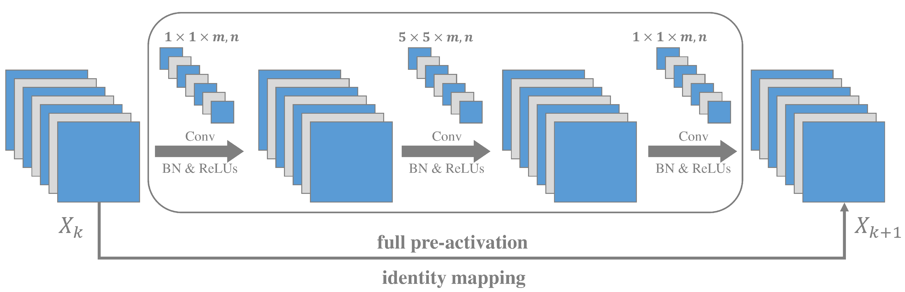
- The proposed CResNet adopts novel residual blocks (RBs) with identity mapping to address the gradient vanishing phenomenon and promotes the discriminant feature learning from multi-sensor datasets.
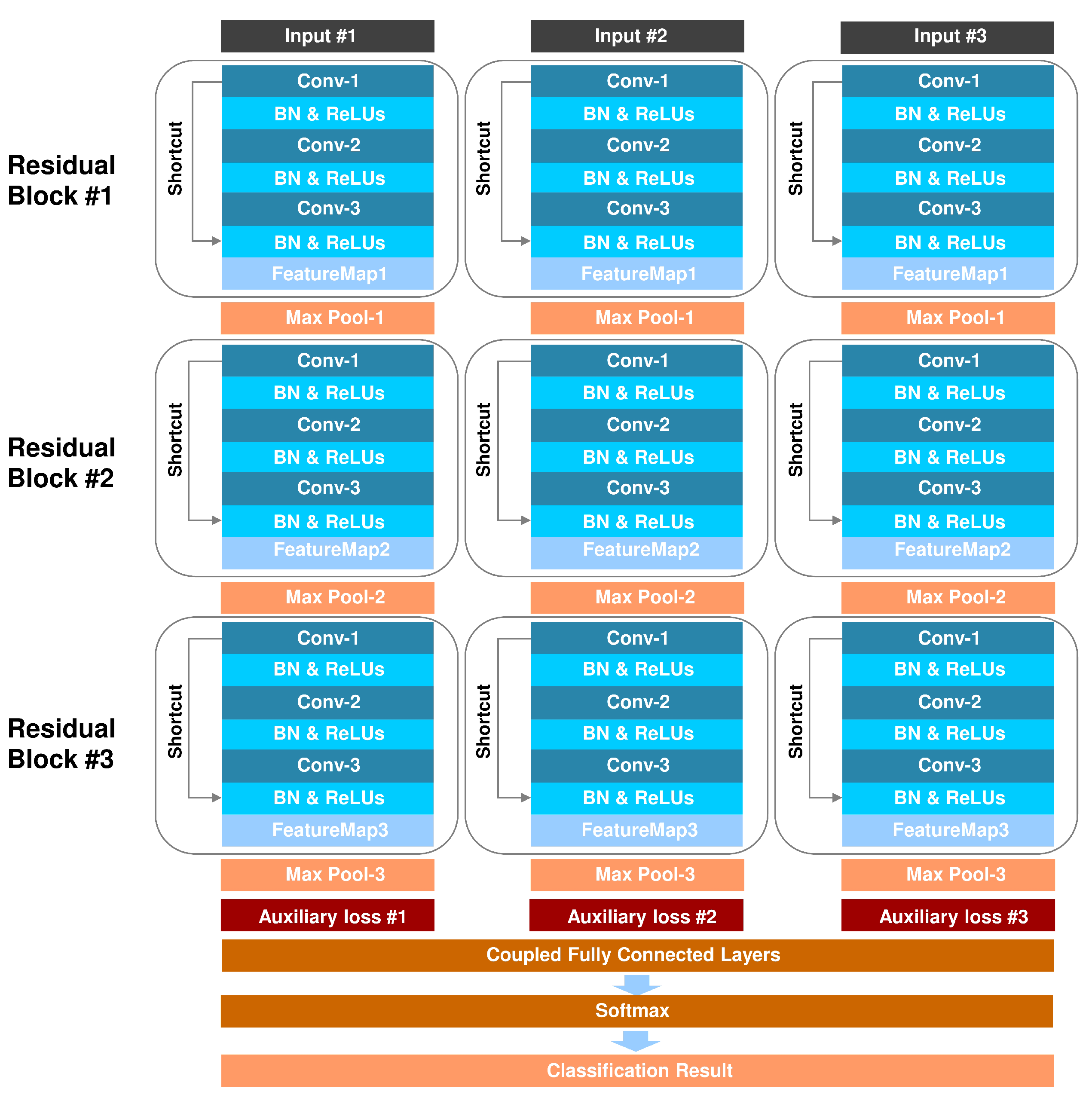
- The design of coupling individual ResNet with auxiliary loss enables the CResNet to simultaneously learn representative features from each dataset by considering an adjusted loss function, and fuse them in a fully automatic end-to-end manner.
- Considering that CResNet is highly modularized and flexible, the proposed framework leads to competitive data fusion performance on three commonly used multi-sensor datasets, where the state-of-the-art classification accuracy are achieved using limited training samples.
2. Methodology
2.1. Feature Learning via Residual Blocks
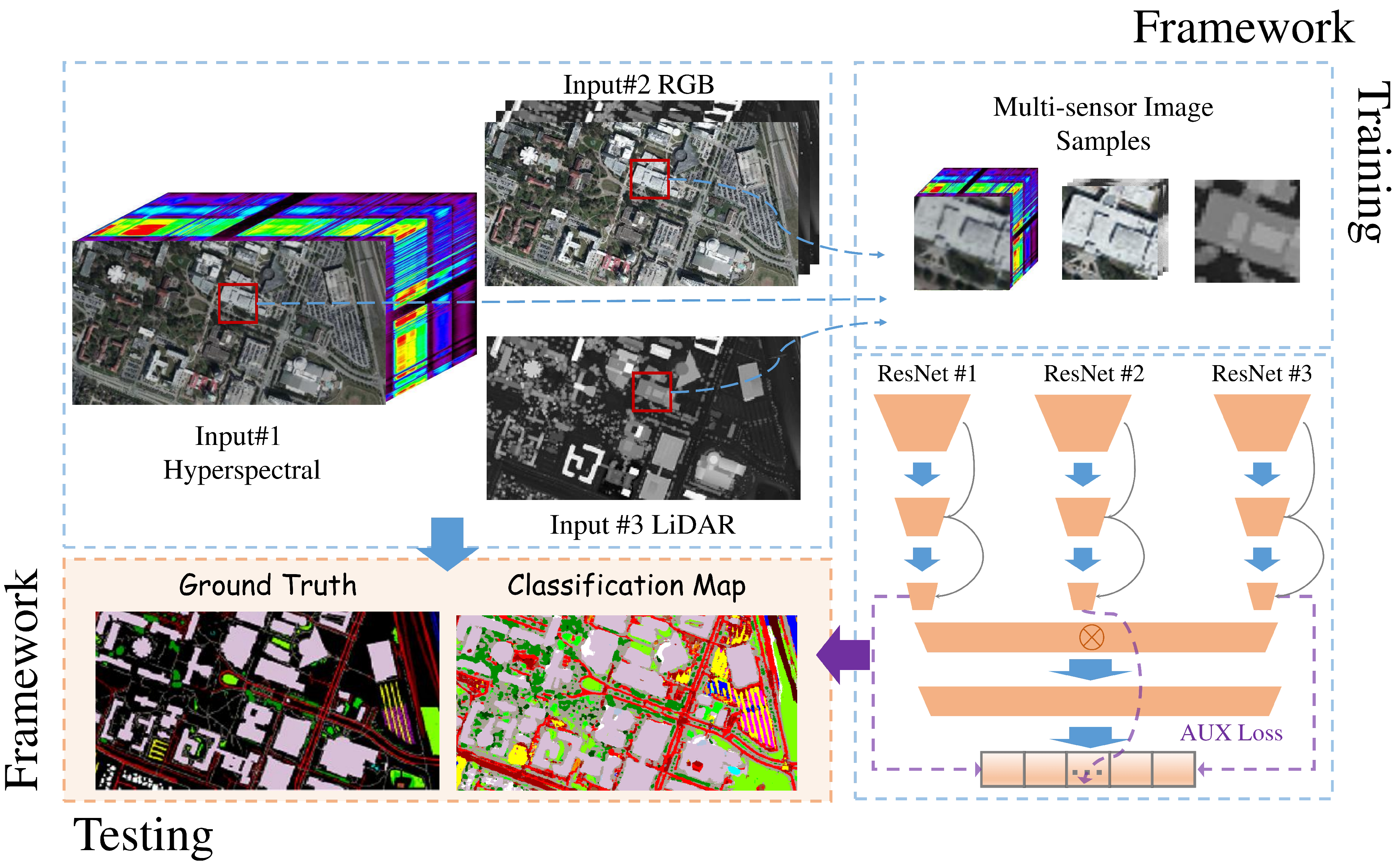
2.2. Multi-Sensor Data Fusion via Coupled ResNets
2.3. Auxiliary Training via Adjusted Loss Function
3. Experiment
3.1. Data Descriptions
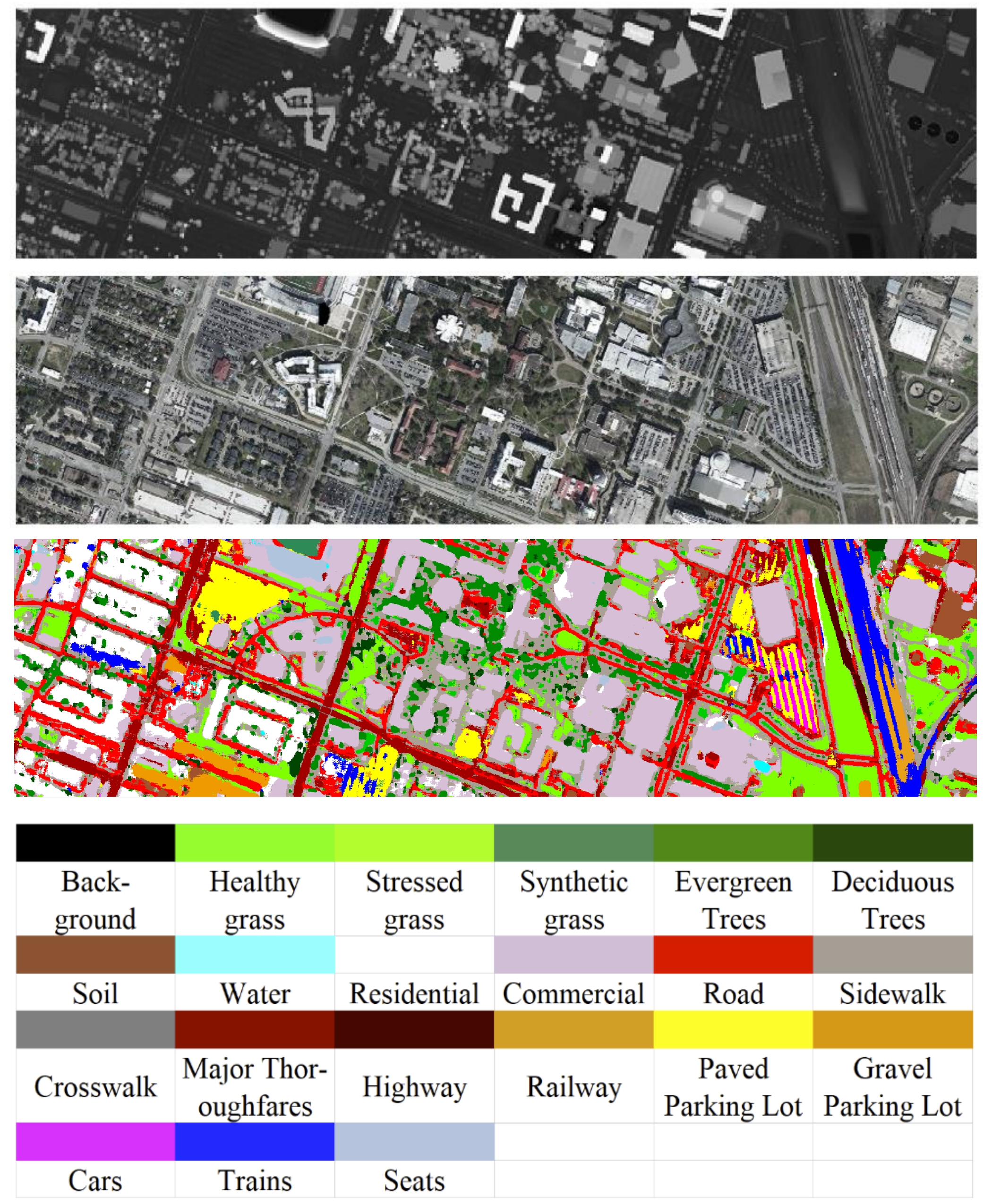
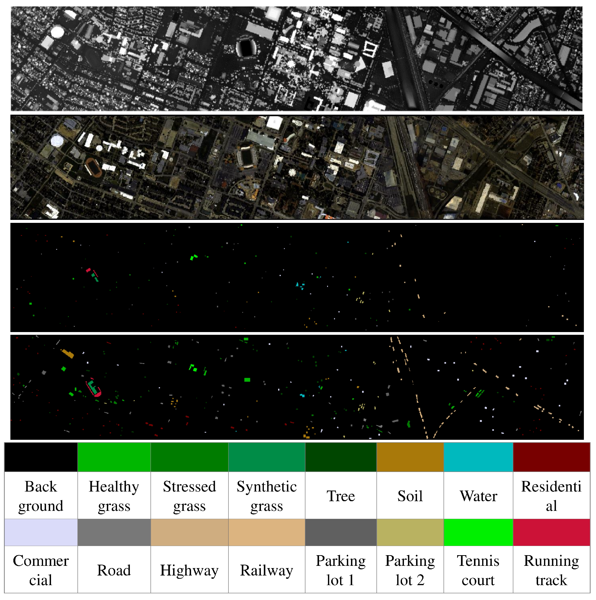
3.1.1. Houston 2013
3.1.2. Houston 2018
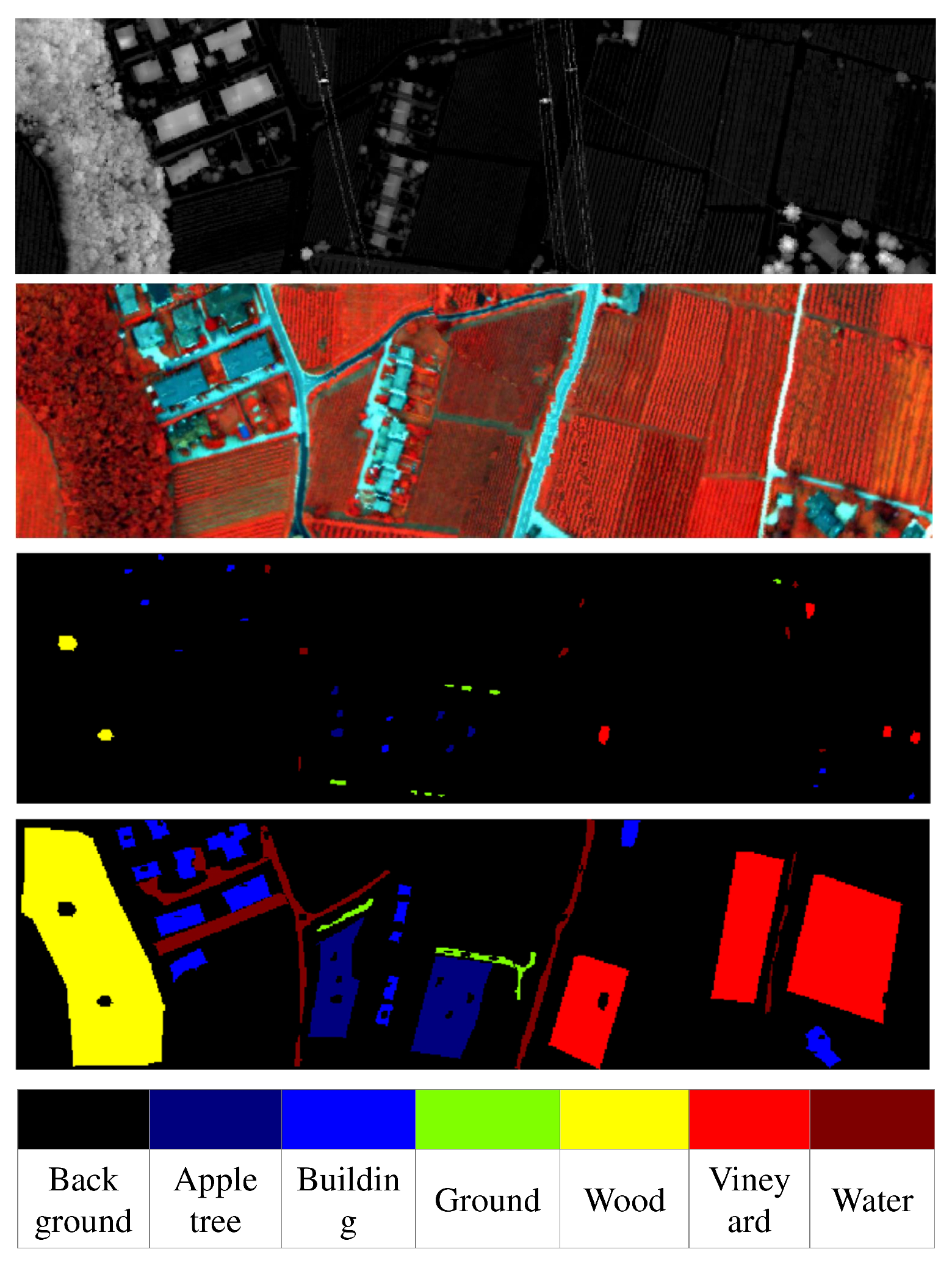
3.1.3. Trento
3.2. Experimental Setup
4. Discussion
4.1. Classification Results
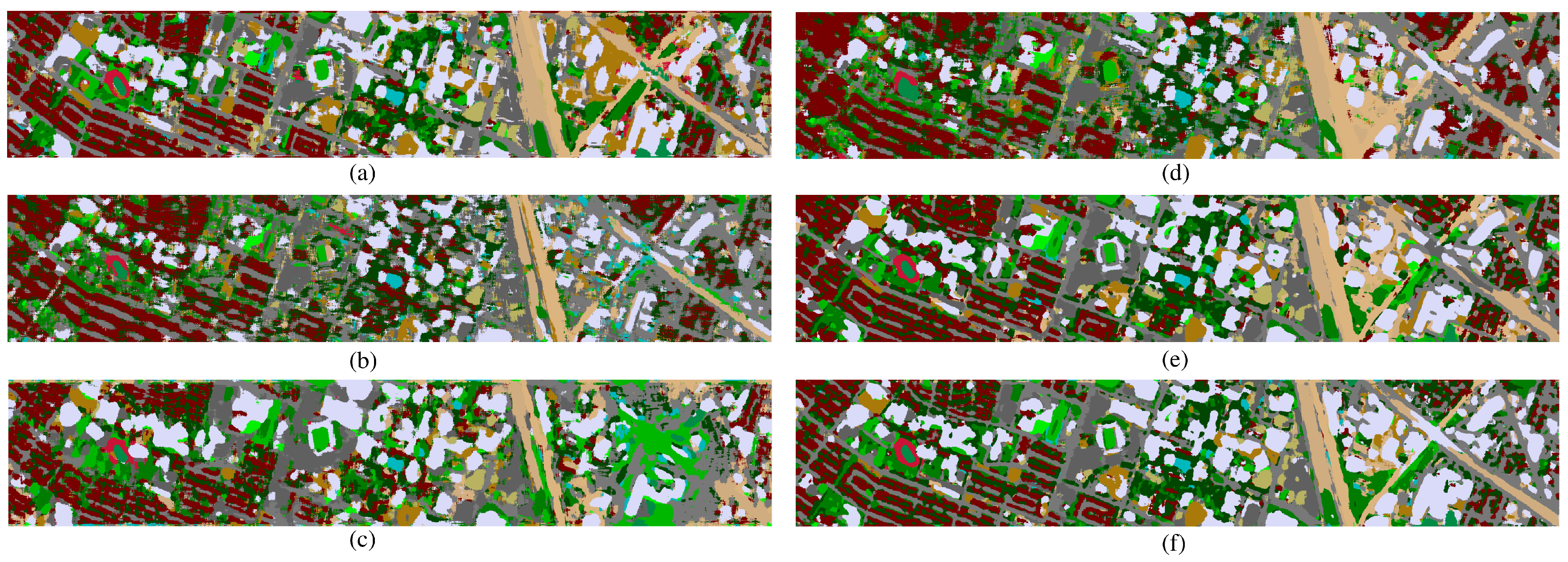
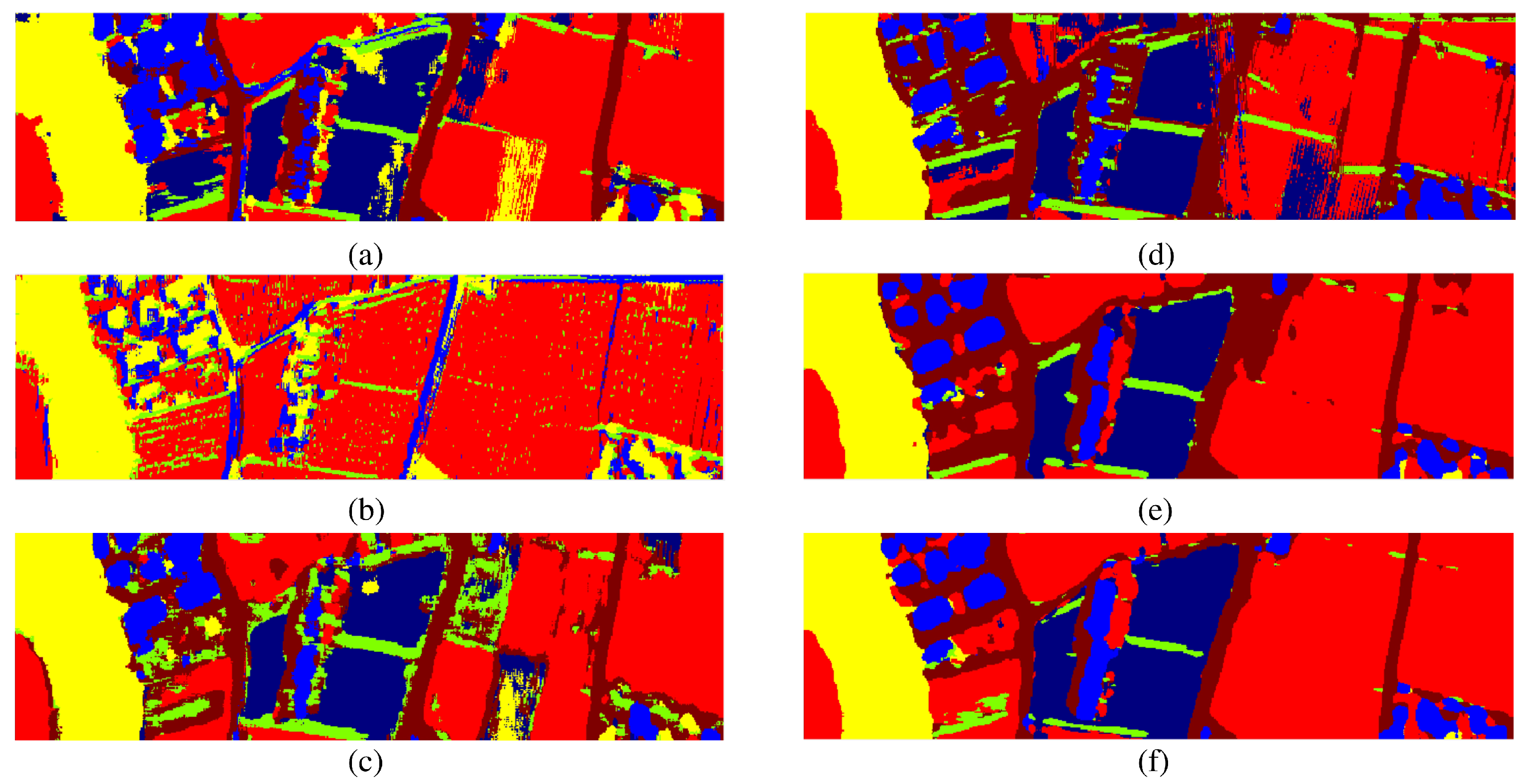
4.1.1. Fusion Performance of Morphological EPs and HSI
- First, it is observed that HSI-ResNet considerably outperforms LiDAR-ResNet for both datasets, which also supports that the redundant spectral-spatial information of HSI has higher discriminative capability than the elevation information of LiDAR data. However, we notice that such discriminative capability of morphological feature (EPs-HSI and EPs-LiDAR) may become relatively uniform, for which EPs-HSI outperforms by 1.24% in the Houston 2013 and EPs-LiDAR outperforms by 2.88% in the Trento dataset. The reason behind this could be that morphological features consist of low-level features based on hand-crafted feature engineering, which not only extracts informative features but also bring high redundancy into feature space, thus the integration of low-level hand-crafted features and high-level deep features can further boost the classification performance [24].
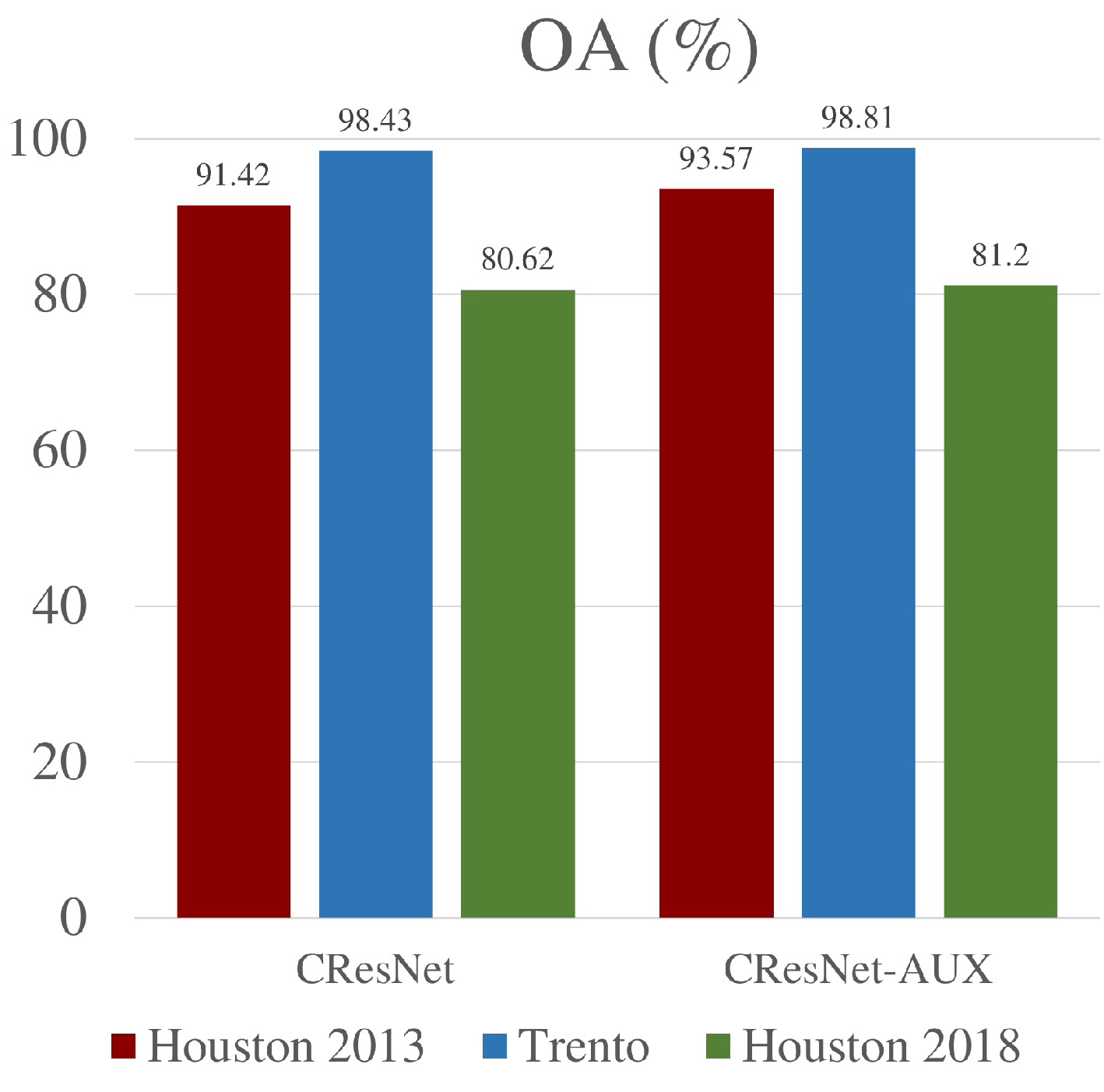
- Second, the fusion of EPs and HSI with CResNet+AUX achieves the best OA (93.57% and 98.81%), AA (93.44% and 94.50%) in both datasets, again confirming the capability and effectiveness of the proposed framework in invariant feature learning from both low-level morphological features and high-level deep features.
- Finally, we observe a common improvement of classification accuracy by training ResNet with adjusted auxiliary loss function. In the Houston 2013 dataset, CResNet-AUX outperforms the original CResNet by producing the highest OA (93.57%) and AA (93.44 %) as well as kappa value of 0.9302. Similar findings are also discovered in the Trento dataset. As explained in Section 2.3, the performance boosting can be attributed to the design of our auxiliary training strategy, where the overall loss function is regularized with the complementary losses from each individual dataset.
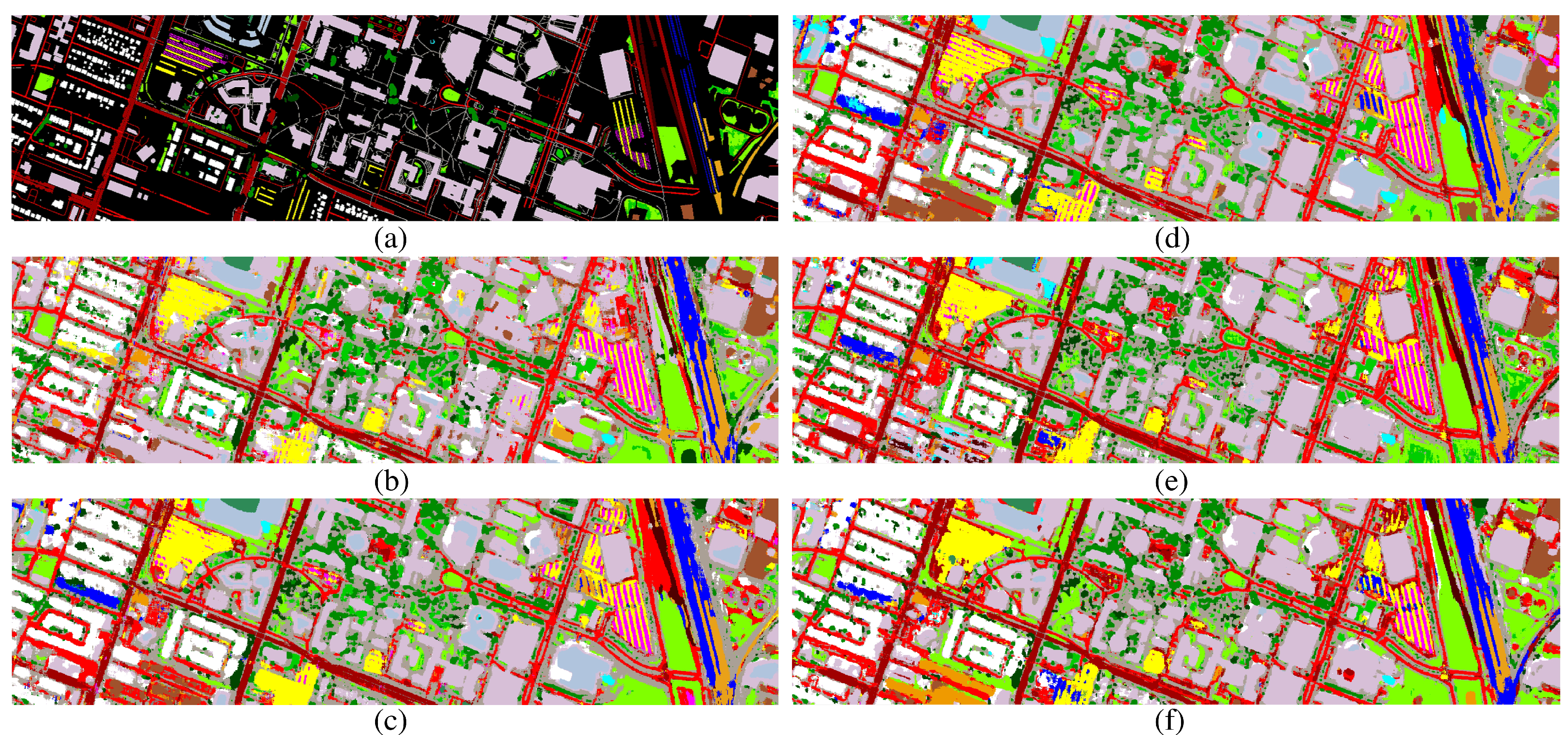
4.1.2. Fusion Performance of RGB, MS LiDAR, and HSI
4.2. Comparison to State-of-the-Art
4.3. The Performance with Respect to the Number of Training Samples
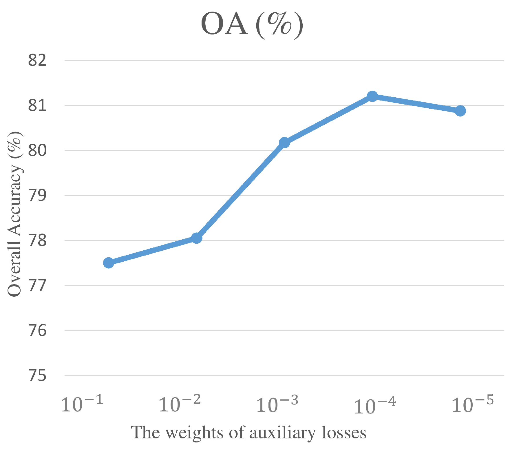
4.4. Sensitivity Analysis of OA with Respect to the Weights of Auxiliary Losses
4.5. Computational Cost
5. Conclusions
- The proposed CResNet fusion framework outperforms all the single sensor-based scenarios in the experiments for all three datasets.
- Both CResNet and CResNet-AUX outperform the state-of-the-art methods for the Houston 2013 dataset.
- The auxiliary training function boosts the performance of CResNet for all the datasets even for the case of limited training samples.
- The proposed CResNet fusion framework shows effective performance when the number of training samples is limited, which is of great importance in the case of applying deep learning techniques for remote sensing datasets.
- The experiments regarding the computational cost justifies the efficiency of the proposed algorithm considering the achievements in the classification accuracies.
Author Contributions
Funding
Acknowledgments
Conflicts of Interest
References
- Ghamisi, P.; Rasti, B.; Yokoya, N.; Wang, Q.; Hofle, B.; Bruzzone, L.; Bovolo, F.; Chi, M.; Anders, K.; Gloaguen, R.; et al. Multisource and Multitemporal Data Fusion in Remote Sensing: A Comprehensive Review of the State of the Art. IEEE Geosci. Remote Sens. Mag. 2019, 7, 6–39. [Google Scholar] [CrossRef] [Green Version]
- Goetz, A.F.H.; Vane, G.; Solomon, J.E.; Rock, B. Imaging Spectrometry for Earth Remote Sensing. Science 1985, 228, 1147–1153. Available online: https://science.sciencemag.org/content/228/4704/1147.full.pdf (accessed on 16 December 2019). [CrossRef]
- Bioucas-Dias, J.M.; Plaza, A.; Camps-Valls, G.; Scheunders, P.; Nasrabadi, N.; Chanussot, J. Hyperspectral Remote Sensing Data Analysis and Future Challenges. IEEE Geosci. Remote Sens. Mag. 2013, 1, 6–36. [Google Scholar] [CrossRef] [Green Version]
- Ghamisi, P.; Yokoya, N.; Li, J.; Liao, W.; Liu, S.; Plaza, J.; Rasti, B.; Plaza, A. Advances in Hyperspectral Image and Signal Processing: A Comprehensive Overview of the State of the Art. IEEE Geosci. Remote Sens. Mag. 2017, 5, 37–78. [Google Scholar] [CrossRef] [Green Version]
- Eitel, J.U.H.; Höfle, B.; Vierling, L.A.; Abellán, A.; Asner, G.P.; Deems, J.S.; Glennie, C.L.; Joerg, P.C.; LeWinter, A.L.; Magney, T.S.; et al. Beyond 3-D: The new spectrum of lidar applications for earth and ecological sciences. Remote. Sens. Environ. 2016, 186, 372–392. [Google Scholar] [CrossRef] [Green Version]
- Höfle, B.; Hollaus, M.; Hagenauer, J. Urban vegetation detection using radiometrically calibrated small-footprint full-waveform airborne LiDAR data. ISPRS J. Photogramm. Remote Sens. 2012, 67, 134–147. [Google Scholar] [CrossRef]
- Anders, K.; Winiwarter, L.; Lindenbergh, R.; Williams, J.G.; Vos, S.E.; Höfle, B. 4D objects-by-change: Spatiotemporal segmentation of geomorphic surface change from LiDAR time series. ISPRS J. Photogramm. Remote Sens. 2020, 159, 352–363. [Google Scholar] [CrossRef]
- Ghamisi, P.; Höfle, B.; Zhu, X.X. Hyperspectral and LiDAR Data Fusion Using Extinction Profiles and Deep Convolutional Neural Network. IEEE J. Sel. Top. Appl. Earth Obs. Remote Sens. 2017, 10, 3011–3024. [Google Scholar] [CrossRef]
- Hänsch, R.; Hellwich, O. Fusion of Multispectral LiDAR, Hyperspectral, and RGB Data for Urban Land Cover Classification. IEEE Geosci. Remote. Sens. Lett. 2020, 1–5. [Google Scholar] [CrossRef]
- Khodadadzadeh, M.; Li, J.; Prasad, S.; Plaza, A. Fusion of Hyperspectral and LiDAR Remote Sensing Data Using Multiple Feature Learning. IEEE J. Sel. Top. Appl. Earth Obs. Remote. Sens. 2015, 8, 2971–2983. [Google Scholar] [CrossRef]
- Pedergnana, M.; Marpu, P.R.; Dalla Mura, M.; Benediktsson, J.A.; Bruzzone, L. Classification of Remote Sensing Optical and LiDAR Data Using Extended Attribute Profiles. IEEE J. Sel. Top. Signal Process. 2012, 6, 856–865. [Google Scholar] [CrossRef]
- Ghamisi, P.; Souza, R.; Benediktsson, J.A.; Zhu, X.X.; Rittner, L.; Lotufo, R.A. Extinction Profiles for the Classification of Remote Sensing Data. IEEE Trans. Geosci. Remote Sens. 2016, 54, 5631–5645. [Google Scholar] [CrossRef]
- Rasti, B.; Ghamisi, P.; Gloaguen, R. Hyperspectral and LiDAR Fusion Using Extinction Profiles and Total Variation Component Analysis. IEEE Trans. Geosci. Remote Sens. 2017, 55, 3997–4007. [Google Scholar] [CrossRef]
- Liao, W.; Pizurica, A.; Bellens, R.; Gautama, S.; Philips, W. Generalized graph-based fusion of hyperspectral and LiDAR data using morphological features. IEEE Geosci. Remote Sens. Lett. 2015, 12, 552–556. [Google Scholar] [CrossRef]
- Rasti, B.; Ghamisi, P.; Plaza, J.; Plaza, A. Fusion of Hyperspectral and LiDAR Data Using Sparse and Low-Rank Component Analysis. IEEE Trans. Geosci. Remote Sens. 2017, 55, 6354–6365. [Google Scholar] [CrossRef] [Green Version]
- Ghamisi, P.; Rasti, B.; Benediktsson, J.A. Multisensor Composite Kernels Based on Extreme Learning Machines. IEEE Geosci. Remote Sens. Lett. 2019, 16, 196–200. [Google Scholar] [CrossRef]
- Zhong, Y.; Cao, Q.; Zhao, J.; Ma, A.; Zhao, B.; Zhang, L. Optimal Decision Fusion for Urban Land-Use/Land-Cover Classification Based on Adaptive Differential Evolution Using Hyperspectral and LiDAR Data. Remote Sens. 2017, 9, 868. [Google Scholar] [CrossRef] [Green Version]
- Xia, J.; Liao, W.; Du, P. Hyperspectral and LiDAR Classification With Semisupervised Graph Fusion. IEEE Geosci. Remote Sens. Lett. 2019, 1–5. [Google Scholar] [CrossRef]
- Jahan, F.; Zhou, J.; Awrangjeb, M.; Gao, Y. Fusion of Hyperspectral and LiDAR Data Using Discriminant Correlation Analysis for Land Cover Classification. IEEE J. Sel. Top. Appl. Earth Obs. Remote Sens. 2018, 11, 3905–3917. [Google Scholar] [CrossRef] [Green Version]
- Hughes, G.F. On the mean accuracy of statistical pattern recognizers. IEEE Trans. Inf. Theory 1968, 14, 55–63. [Google Scholar] [CrossRef] [Green Version]
- Li, S.; Song, W.; Fang, L.; Chen, Y.; Ghamisi, P.; Benediktsson, J.A. Deep Learning for Hyperspectral Image Classification: An Overview. IEEE Trans. Geosci. Remote Sens. 2019, 57, 6690–6709. [Google Scholar] [CrossRef] [Green Version]
- Rasti, B.; Hong, D.; Hang, R.; Ghamisi, P.; Kang, X.; Chanussot, J.; Benediktsson, J.A. Feature Extraction for Hyperspectral Imagery: The Evolution from Shallow to Deep (Overview and Toolbox). IEEE Geosci. Remote Sens. Mag. 2020. [Google Scholar] [CrossRef]
- Chen, Y.; Li, C.; Ghamisi, P.; Jia, X.; Gu, Y. Deep Fusion of Remote Sensing Data for Accurate Classification. IEEE Geosci. Remote Sens. Lett. 2017, 14, 1253–1257. [Google Scholar] [CrossRef]
- Li, H.; Ghamisi, P.; Soergel, U.; Zhu, X.X. Hyperspectral and LiDAR Fusion Using Deep Three-Stream Convolutional Neural Networks. Remote Sens. 2018, 10, 1649. [Google Scholar] [CrossRef] [Green Version]
- Xu, X.; Li, W.; Ran, Q.; Du, Q.; Gao, L.; Zhang, B. Multisource Remote Sensing Data Classification Based on Convolutional Neural Network. IEEE Trans. Geosci. Remote Sens. 2018, 56, 937–949. [Google Scholar] [CrossRef]
- Qiu, C.; Schmitt, M.; Mou, L.; Ghamisi, P.; Zhu, X.X. Feature Importance Analysis for Local Climate Zone Classification Using a Residual Convolutional Neural Network with Multi-Source Datasets. Remote Sens. 2018, 10, 1572. [Google Scholar] [CrossRef] [Green Version]
- Zhang, M.; Li, W.; Du, Q.; Gao, L.; Zhang, B. Feature Extraction for Classification of Hyperspectral and LiDAR Data Using Patch-to-Patch CNN. IEEE Trans. Cybern. 2020, 50, 100–111. [Google Scholar] [CrossRef]
- Xu, S.; Amira, O.; Liu, J.; Zhang, C.; Zhang, J.; Li, G. HAM-MFN: Hyperspectral and Multispectral Image Multiscale Fusion Network With RAP Loss. IEEE Trans. Geosci. Remote Sens. 2020, 1–11. [Google Scholar] [CrossRef]
- He, K.; Zhang, X.; Ren, S.; Sun, J. Deep Residual Learning for Image Recognition. In Proceedings of the 2016 IEEE Conference on Computer Vision and Pattern Recognition (CVPR), Las Vegas, NV, USA, 26 June–1 July 2016; pp. 770–778. [Google Scholar] [CrossRef] [Green Version]
- He, K.; Zhang, X.; Ren, S.; Sun, J. Identity Mappings in Deep Residual Networks. In Computer Vision – ECCV 2016; Leibe, B., Matas, J., Sebe, N., Welling, M., Eds.; Springer International Publishing: Cham, Switzerland, 2016; pp. 630–645. [Google Scholar]
- Zhong, Z.; Li, J.; Luo, Z.; Chapman, M. Spectral–Spatial Residual Network for Hyperspectral Image Classification: A 3-D Deep Learning Framework. IEEE Trans. Geosci. Remote Sens. 2018, 56, 847–858. [Google Scholar] [CrossRef]
- Qiu, C.; Mou, L.; Schmitt, M.; Zhu, X.X. Fusing Multiseasonal Sentinel-2 Imagery for Urban Land Cover Classification With Multibranch Residual Convolutional Neural Networks. IEEE Geosci. Remote Sens. Lett. 2020, 1–5. [Google Scholar] [CrossRef]
- Ioffe, S.; Szegedy, C. Batch Normalization: Accelerating Deep Network Training by Reducing Internal Covariate Shift. In Proceedings of the 32nd International Conference on Machine Learning, Lille, France, 6–11 July 2015; Bach, F., Blei, D., Eds.; PMLR: Lille, France, 2015; Volume 37, pp. 448–456. [Google Scholar]
- Nair, V.; Hinton, G.E. Rectified Linear Units Improve Restricted Boltzmann Machines. In Proceedings of the 27th International Conference on Machine Learning (ICML 2010), Haifa, Israel, 21–24 June 2010. [Google Scholar]
- Chen, Y.H.; Jiang, C.L.; Jia, X.; Ghamisi, P. Deep Feature Extraction and Classification of Hyperspectral Images Based on Convolutional Neural Networks. IEEE Trans. Geosci. Remote Sens. 2016, 54, 6232–6250. [Google Scholar] [CrossRef] [Green Version]
- Ghamisi, P.; Souza, R.; Benediktsson, J.A.; Rittner, L.; Lotufo, R.; Zhu, X.X. Hyperspectral Data Classification Using Extended Extinction Profiles. IEEE Geosci. Remote Sens. Lett. 2016, 13, 1641–1645. [Google Scholar] [CrossRef] [Green Version]
- Szegedy, C.; Liu, W.; Jia, Y.; Sermanet, P.; Reed, S.; Anguelov, D.; Erhan, D.; Vanhoucke, V.; Rabinovich, A. Going deeper with convolutions. In Proceedings of the 2015 IEEE Conference on Computer Vision and Pattern Recognition (CVPR), Boston, MA, USA, 7–12 June 2015; pp. 1–9. [Google Scholar] [CrossRef] [Green Version]
- Debes, C.; Merentitis, A.; Heremans, R.; Hahn, J.; Frangiadakis, N.; van Kasteren, T.; Liao, W.; Bellens, R.; Pizurica, A.; Gautama, S.; et al. Hyperspectral and LiDAR Data Fusion: Outcome of the 2013 GRSS Data Fusion Contest. IEEE J. Sel. Top. Appl. Earth Obs. Remote Sens. 2014, 7, 2405–2418. [Google Scholar] [CrossRef]
- Xu, Y.; Du, B.; Zhang, L.; Cerra, D.; Pato, M.; Carmona, E.; Prasad, S.; Yokoya, N.; Hänsch, R.; Le Saux, B. Advanced Multi-Sensor Optical Remote Sensing for Urban Land Use and Land Cover Classification: Outcome of the 2018 IEEE GRSS Data Fusion Contest. IEEE J. Sel. Top. Appl. Earth Obs. Remote Sens. 2019, 12, 1709–1724. [Google Scholar] [CrossRef]


| Class No. | Class Name | Training | Testing | Samples |
|---|---|---|---|---|
| 1 | Healthy grass | 198 | 1053 | 1251 |
| 2 | Stressed grass | 190 | 1064 | 1254 |
| 3 | Synthetic grass | 192 | 505 | 697 |
| 4 | Tree | 188 | 1056 | 1244 |
| 5 | Soil | 186 | 1056 | 1242 |
| 6 | Water | 182 | 143 | 325 |
| 7 | Residential | 196 | 1072 | 1268 |
| 8 | Commercial | 191 | 1053 | 1244 |
| 9 | Road | 193 | 1059 | 1252 |
| 10 | Highway | 191 | 1036 | 1227 |
| 11 | Railway | 181 | 1054 | 1235 |
| 12 | Parking Lot 1 | 192 | 1041 | 1233 |
| 13 | Parking Lot 2 | 184 | 285 | 469 |
| 14 | Tennis court | 181 | 247 | 428 |
| 15 | Running track | 187 | 473 | 660 |
| Total | 2832 | 12,197 | 15,029 |
| Class No. | Class Name | Training | Testing | Samples |
|---|---|---|---|---|
| 1 | Healthy grass | 1458 | 8341 | 9799 |
| 2 | Stressed grass | 4316 | 28,186 | 32,502 |
| 3 | Synthetic grass | 331 | 353 | 684 |
| 4 | Evergreen Trees | 2005 | 11,583 | 13,588 |
| 5 | Deciduous Trees | 676 | 4372 | 5048 |
| 6 | Soil | 1757 | 2759 | 4516 |
| 7 | Water | 147 | 119 | 266 |
| 8 | Residential | 3809 | 35,953 | 39,762 |
| 9 | Commercial | 2789 | 220,895 | 223,684 |
| 10 | Road | 3188 | 42,622 | 45,810 |
| 11 | Sidewalk | 2699 | 31,303 | 34,002 |
| 12 | Crosswalk | 225 | 1291 | 1516 |
| 13 | Major Thoroughfares | 5193 | 41,165 | 46,358 |
| 14 | Highway | 700 | 9149 | 9849 |
| 15 | Railway | 1224 | 5713 | 6937 |
| 16 | Paved Parking Lot | 1179 | 10,296 | 11,475 |
| 17 | Gravel Parking Lot | 127 | 22 | 149 |
| 18 | Cars | 848 | 5730 | 6578 |
| 19 | Trains | 493 | 4872 | 5365 |
| 20 | Seats | 1313 | 5511 | 6824 |
| Total | 34,477 | 470,235 | 504,712 |
| Class No. | Class Name | Training | Testing | Samples |
|---|---|---|---|---|
| 1 | Apple trees | 129 | 3905 | 4034 |
| 2 | Buildings | 125 | 2778 | 2903 |
| 3 | Ground | 105 | 374 | 479 |
| 4 | Wood | 154 | 8969 | 9123 |
| 5 | Vineyard | 184 | 10,317 | 10,501 |
| 6 | Roads | 122 | 3052 | 3174 |
| Total | 819 | 29,395 | 30,214 |
| # | Class | HSI-ResNet | LiDAR-ResNet | EPs-HSI-ResNet | EPs-LiDAR-ResNet | CResNet | CResNet-AUX |
|---|---|---|---|---|---|---|---|
| Number of features | (144) | (1) | (225) | (71) | (144+225+71) | (144+225+71) | |
| 1 | Healthy grass | 77.68 | 51.76 | 74.83 | 54.13 | 83.00 | 86.51 |
| 2 | Stressed grass | 98.59 | 47.09 | 76.60 | 56.77 | 99.81 | 98.01 |
| 3 | Synthetic grass | 86.53 | 87.33 | 87.33 | 94.06 | 84.36 | 87.87 |
| 4 | Tree | 86.46 | 51.52 | 51.89 | 68.09 | 96.69 | 85.52 |
| 5 | Soil | 89.11 | 43.56 | 93.94 | 52.37 | 99.91 | 87.02 |
| 6 | Water | 81.12 | 78.32 | 91.61 | 79.02 | 95.80 | 99.81 |
| 7 | Residential | 93.75 | 67.07 | 74.07 | 75.93 | 90.11 | 100.00 |
| 8 | Commercial | 81.86 | 75.12 | 80.53 | 83.57 | 95.73 | 95.72 |
| 9 | Road | 88.67 | 58.55 | 55.71 | 59.87 | 90.65 | 96.68 |
| 10 | Highway | 74.52 | 73.84 | 54.05 | 72.78 | 70.46 | 100.00 |
| 11 | Railway | 95.64 | 90.32 | 68.98 | 98.29 | 94.68 | 85.54 |
| 12 | Parking Lot 1 | 85.78 | 68.20 | 73.20 | 78.10 | 97.50 | 95.80 |
| 13 | Parking Lot 2 | 82.81 | 75.44 | 68.07 | 72.28 | 79.30 | 94.05 |
| 14 | Tennis court | 100.00 | 90.28 | 93.12 | 88.66 | 100.00 | 95.10 |
| 15 | Running track | 68.92 | 39.32 | 41.23 | 15.43 | 89.85 | 93.87 |
| OA(%) | 86.60 | 63.82 | 70.63 | 69.39 | 91.42 | 93.57 | |
| AA(%) | 86.10 | 66.51 | 72.34 | 69.96 | 91.19 | 93.44 | |
| Kappa | 0.8545 | 0.6074 | 0.6809 | 0.6676 | 0.9068 | 0.9302 |
| # | Class | HSI-ResNet | LiDAR-ResNet | EPs-HSI-ResNet | EPs-LiDAR-ResNet | CResNet | CResNet-AUX |
|---|---|---|---|---|---|---|---|
| Number of Features | (63) | (1) | (225) | (71) | (63+225+71) | (63+225+71) | |
| 1 | Apple trees | 98.21 | 0.00 | 96.67 | 98.39 | 98.10 | 99.74 |
| 2 | Buildings | 93.12 | 15.77 | 87.83 | 97.52 | 97.77 | 99.60 |
| 3 | Ground | 77.54 | 39.84 | 77.01 | 64.71 | 77.01 | 75.40 |
| 4 | Wood | 98.99 | 98.27 | 99.74 | 100.00 | 99.90 | 100.00 |
| 5 | Vineyard | 99.96 | 97.00 | 94.92 | 97.77 | 100.00 | 100.00 |
| 6 | Roads | 60.52 | 2.62 | 75.75 | 83.65 | 92.46 | 92.27 |
| OA (%) | 94.40 | 66.30 | 93.74 | 96.62 | 98.43 | 98.81 | |
| AA (%) | 88.06 | 42.25 | 88.65 | 90.34 | 94.21 | 94.50 | |
| Kappa | 0.9250 | 0.5178 | 0.9166 | 0.9548 | 0.9790 | 0.9841 |
| # | Class | HSI-ResNet | LiDAR-ResNet | RGB-ResNet | CResNet | CResNet-AUX |
|---|---|---|---|---|---|---|
| Number of features | (48) | (7) | (3) | (48+7+3) | (48+7+3) | |
| 1 | Healthy grass | 46.35 | 24.25 | 41.54 | 18.77 | 75.90 |
| 2 | Stressed grass | 79.64 | 74.80 | 79.37 | 90.43 | 67.79 |
| 3 | Synthetic grass | 82.72 | 100.00 | 100.00 | 100.00 | 100.00 |
| 4 | Evergreen Trees | 93.59 | 90.02 | 93.05 | 94.74 | 95.24 |
| 5 | Deciduous Trees | 46.27 | 43.62 | 44.26 | 59.54 | 59.47 |
| 6 | Soil | 36.17 | 31.39 | 86.48 | 43.82 | 36.82 |
| 7 | Water | 42.02 | 0.00 | 22.69 | 30.25 | 1.68 |
| 8 | Residential | 89.86 | 87.51 | 91.08 | 90.79 | 88.00 |
| 9 | Commercial | 71.24 | 70.89 | 66.35 | 92.71 | 92.75 |
| 10 | Road | 54.44 | 61.35 | 65.97 | 64.14 | 72.77 |
| 11 | Sidewalk | 63.14 | 73.80 | 75.18 | 62.26 | 71.27 |
| 12 | Crosswalk | 3.95 | 2.40 | 2.87 | 3.02 | 3.95 |
| 13 | Major Thoroughfares | 47.50 | 62.67 | 56.97 | 65.15 | 57.62 |
| 14 | Highway | 31.82 | 34.97 | 37.22 | 42.34 | 44.82 |
| 15 | Railway | 77.58 | 84.75 | 84.74 | 63.77 | 63.96 |
| 16 | Paved parking Lot | 85.60 | 97.31 | 94.80 | 83.64 | 89.48 |
| 17 | Gravel parking Lot | 100.00 | 100.00 | 100.00 | 100.00 | 100.00 |
| 18 | Cars | 32.24 | 37.24 | 50.89 | 29.91 | 34.57 |
| 19 | Trains | 93.49 | 99.36 | 98.75 | 92.44 | 97.74 |
| 20 | Seats | 63.49 | 99.84 | 98.42 | 61.13 | 73.42 |
| OA (%) | 67.83 | 70.26 | 69.53 | 80.62 | 81.20 | |
| AA (%) | 62.16 | 63.81 | 69.53 | 64.47 | 66.36 | |
| Kappa | 0.5944 | 0.6287 | 0.6253 | 0.7416 | 0.7506 |
| Methods | MLRsub [10] | OTVCA [13] | SLRCA [15] | DeepFusion [23] | EPs-CNN [8] | CK-CNN [24] | CResNet | CResNet-AUX |
|---|---|---|---|---|---|---|---|---|
| OA (%) | 92.05 | 92.45 | 91.30 | 91.32 | 91.02 | 92.57 | 91.42 | 93.57 |
| AA (%) | 92.85 | 92.68 | 91.95 | 91.96 | 91.82 | 92.48 | 91.19 | 93.44 |
| Kappa | 0.9137 | 0.9181 | 0.9056 | 0.9057 | 0.9033 | 0.9193 | 0.9068 | 0.9302 |
| Houston 2013 | HSI-ResNet | LiDAR-ResNet | EPs-HSI-ResNet | EPs-LiDAR-ResNet | CResNet | CResNet-AUX |
| Train (min) | 8.84 | 5.837 | 8.61 | 5.67 | 16.11 | 16.61 |
| Test (s) | 4.38 | 3.04 | 5.53 | 3.61 | 8.15 | 16.25 |
| Trento | HSI-ResNet | LiDAR-ResNet | EPs-HSI-ResNet | EPs-LiDAR-ResNet | CResNet | CResNet-AUX |
| Train (min) | 5.69 | 5.04 | 6.88 | 5.79 | 11.73 | 13.66 |
| Test (s) | 6.28 | 5.62 | 9.15 | 7.13 | 13.57 | 14.06 |
| Houston 2018 | HSI-ResNet | LiDAR-ResNet | RGB-ResNet | CResNet | CResNet-AUX | |
| Train (min) | 82.50 | 63.11 | 58.13 | 159.9 | 168.33 | |
| Test (s) | 53.64 | 35.84 | 38.38 | 102.91 | 107.79 |
© 2020 by the authors. Licensee MDPI, Basel, Switzerland. This article is an open access article distributed under the terms and conditions of the Creative Commons Attribution (CC BY) license (http://creativecommons.org/licenses/by/4.0/).
Share and Cite
Li, H.; Ghamisi, P.; Rasti, B.; Wu, Z.; Shapiro, A.; Schultz, M.; Zipf, A. A Multi-Sensor Fusion Framework Based on Coupled Residual Convolutional Neural Networks. Remote Sens. 2020, 12, 2067. https://0-doi-org.brum.beds.ac.uk/10.3390/rs12122067
Li H, Ghamisi P, Rasti B, Wu Z, Shapiro A, Schultz M, Zipf A. A Multi-Sensor Fusion Framework Based on Coupled Residual Convolutional Neural Networks. Remote Sensing. 2020; 12(12):2067. https://0-doi-org.brum.beds.ac.uk/10.3390/rs12122067
Chicago/Turabian StyleLi, Hao, Pedram Ghamisi, Behnood Rasti, Zhaoyan Wu, Aurelie Shapiro, Michael Schultz, and Alexander Zipf. 2020. "A Multi-Sensor Fusion Framework Based on Coupled Residual Convolutional Neural Networks" Remote Sensing 12, no. 12: 2067. https://0-doi-org.brum.beds.ac.uk/10.3390/rs12122067