Article

Comparison of Object Detection and Patch-Based Classification Deep Learning Models on Mid- to Late-Season Weed Detection in UAV Imagery

1
Department of Biological Systems Engineering, University of Nebraska-Lincoln, Lincoln, NE 68583, USA
2
Department of Computer Science and Engineering, University of Nebraska-Lincoln, Lincoln, NE 68588, USA
3
Department of Electrical and Computer Engineering, University of Nebraska-Lincoln, Lincoln, NE 68588, USA
4
Department of Agronomy and Horticulture, University of Nebraska-Lincoln, Lincoln, NE 68583, USA
*
Author to whom correspondence should be addressed.
Remote Sens. 2020, 12(13), 2136; https://0-doi-org.brum.beds.ac.uk/10.3390/rs12132136
Submission received: 30 April 2020 / Revised: 28 June 2020 / Accepted: 29 June 2020 / Published: 3 July 2020
(This article belongs to the Special Issue UAVs for Vegetation Monitoring)

Abstract

:
Mid- to late-season weeds that escape from the routine early-season weed management threaten agricultural production by creating a large number of seeds for several future growing seasons. Rapid and accurate detection of weed patches in field is the first step of site-specific weed management. In this study, object detection-based convolutional neural network models were trained and evaluated over low-altitude unmanned aerial vehicle (UAV) imagery for mid- to late-season weed detection in soybean fields. The performance of two object detection models, Faster RCNN and the Single Shot Detector (SSD), were evaluated and compared in terms of weed detection performance using mean Intersection over Union (IoU) and inference speed. It was found that the Faster RCNN model with 200 box proposals had similar good weed detection performance to the SSD model in terms of precision, recall, f1 score, and IoU, as well as a similar inference time. The precision, recall, f1 score and IoU were 0.65, 0.68, 0.66 and 0.85 for Faster RCNN with 200 proposals, and 0.66, 0.68, 0.67 and 0.84 for SSD, respectively. However, the optimal confidence threshold of the SSD model was found to be much lower than that of the Faster RCNN model, which indicated that SSD might have lower generalization performance than Faster RCNN for mid- to late-season weed detection in soybean fields using UAV imagery. The performance of the object detection model was also compared with patch-based CNN model. The Faster RCNN model yielded a better weed detection performance than the patch-based CNN with and without overlap. The inference time of Faster RCNN was similar to patch-based CNN without overlap, but significantly less than patch-based CNN with overlap. Hence, Faster RCNN was found to be the best model in terms of weed detection performance and inference time among the different models compared in this study. This work is important in understanding the potential and identifying the algorithms for an on-farm, near real-time weed detection and management.

1. Introduction

Weeds are unwanted plants that grow in the field and compete with the crops for water, light, nutrients, and space. If uncontrolled, weeds can have several negative consequences, such as crop yield loss, production of a large number of seeds thereby creating a weed seed bank in the field, and contamination of grain during harvesting [1,2]. Traditionally, weed management programs involve the control of weeds through chemical or mechanical means such as the uniform application of herbicides throughout the field. However, the spatial density of weeds is not uniform across the field, thereby leading to overuse of chemicals which results in environmental concerns and evolution of herbicide-resistant weeds. To overcome this issue, a concept of site-specific weed management (SSWM), which refers to detecting weed patches and spot spraying or removal by mechanical means, was proposed in the early 1990s [3,4,5]. Weed control early in the season is critical, since otherwise the weeds would compete with the crops for resources during the critical growth stage of the crops resulting in possible yield loss [6,7]. Therefore, in addition to the application of pre-emergence herbicides, the early application of post emergence herbicides is preferred for effective weed control and also to reduce the damage to crops. The effectiveness of weed control from post-emergence herbicides depends on the timing of application [8,9]. Detection of early season weeds in an accurate and timely manner helps in the creation of prescription maps for the site-specific application of post-emergence herbicides [10,11,12]. Prescription maps for post-emergence application can also be created from late-season weeds detected during the previous seasons [13,14,15,16,17]. Compared to early season weeds, late-season weeds do not directly affect the yield of the crop, since it is not competing for resources during the critical growth period of the crop. However, if unattended, late-season weeds can produce large numbers of seeds creating problems in the subsequent growing seasons. Therefore, the detection and control of late-season weeds can be complementary to early season weed control.
Earlier studies on weed detection often used Color Co-occurrence Matrix-based texture analysis for digital images [18,19]. Following this, there were several studies on combining optical sensing, image processing algorithms, and variable rate application implements for real-time site-specific herbicide application on weeds. However, the speed of these systems was limited by computational power constraints for real-time detection, which in turn limited their ability to cover large areas of fields [20]. Unmanned aerial vehicles (UAVs) with their ability to cover large areas in a short amount of time and payload capacity to carry optical sensors provide an alternative. UAVs have been studied for various applications in precision farming such as weed, disease, pest, biotic and abiotic stress detection using high-resolution aerial imagery [21,22,23,24]. Several studies have investigated the potential of using remote sensing to discriminate between crops and weeds for weed mapping at different phenological stages and found that results differ based on the phenology [2,10,25,26,27,28,29,30,31,32,33]. The similar spectral signature of the crops and the weeds, occurrence of weeds as small patches and interference of soil pixels in detection are the major challenges for remote sensing in early season weed detection [2,12]. A common approach is to use vegetation indices to segment the vegetation pixels from the soil pixels, followed by crop row detection for weed classification using techniques such as object-based image analysis (OBIA) and Hough Transform [29,32,34]. However, crop row detection-based approaches cannot detect intra-row weeds. Hence, machine learning based classifiers using features computed from OBIA were used to detect intra-row weeds as well [10]. However, the performance of OBIA is sensitive to the segmentation accuracy and so optimal parameters for the segmentation step in OBIA have to be found for different crops and field conditions [35].
With advancements in parallel computing and the availability of large datasets, convolutional neural networks (CNN) were found to perform very well in computer vision tasks such as classification, prediction, and object detection [36]. In addition to performance, another principal advantage of CNN is that the network learns the features by itself during the training process, and hence manual feature engineering is not necessary. CNNs have been studied for various image-based applications in agriculture such as weed detection, disease detection, fruit counting, crop yield estimation, obstacle detection for autonomous farm machines, and soil moisture content estimation [37,38,39,40,41]. CNNs have been used for weed detection using data obtained in three different ways—using UAVs, using the autonomous ground robot, and high-resolution images obtained manually in the field. A simple CNN binary classifier was trained to classify manually collected small high-resolution images of maize and weeds [42,43]. The performance of the classifier with transfer learning on various pre-trained networks such as LeNet and AlexNet was compared, but this study was limited in variability in the obtained dataset and on the evaluation of the classification approach with large images. Dyrmann et al. [23] used a pre-trained VGG-16 network and replaced the fully connected layer with a deconvolution layer to output a pixel-wise classification map of maize, weeds, and soil. The training images were simulated by overlapping a small number of available images of soil, maize, and weeds with various sizes and orientations. The use of an encoder-decoder architecture for real-time output of pixel-wise classification maps for site-specific spraying was studied. It was found that by adding hand-crafted features such as vegetation indices, different color spaces, and edges as input channels to CNN, the model’s ability to generalize to different locations and at the different growth stages of the crop improved [44,45,46]. Furthermore, to improve the generalization performance of the CNN-based weed detection system, Lottes et al. [25] studied the use of fully-convolutional DenseNet with spatiotemporal fusion and spatiotemporal decoder with sequential images to learn the local geometry of crops in fixed straight lines along the path of a ground robot. In the case of overlapping crop and weed objects, Lottes et al. [15] proposed a key point based feature extraction approach that was used to detect weed objects that overlap with the crop. In addition to weed detection, for effective removal of weeds using mechanical or laser-based methods, it is necessary to detect the stem location of weeds prior to actuation. A fully-convolutional DenseNet was trained to output the stem location as well as a pixel-wise segmentation map of crops and weeds [47,48].
In the case of weed detection using UAV imagery, similar to OBIA approaches mentioned above, dos Santos Ferreira et al. [3] used a Superpixel segmentation algorithm to segment objects and trained a CNN to classify these clusters. They then compared the performance with other machine learning classifiers which use handcrafted features. Sa et al. [27] studied the use of an encoder-decoder architecture, Segnet, for the pixel-wise classification of multispectral imagery and followed up with a performance evaluation of this detection system using different UAV platforms and multispectral cameras [49,50,51]. Bah et al. [29] used the Hough transform along with a patch-based CNN to detect weeds from UAV imagery and found that overlapping weed and crop objects led to some errors in this approach. It is to be noted that, in this approach, the patches are sliced from the large image in a non-overlapping manner. Huang et al. [30] studied the performance of various deep learning architectures for pixel-wise classification of rice and weeds and found that the fully-convolutional network architecture outperformed other architectures. Yu et al. [52] studied the use of CNN for multispecies weed detection in rye grass.
From the literature reviewed, it can be seen that automated weed detection has been primarily focused on early season weeds, since that is found to be the critical period for weed management and to prevent crop yield loss. However, it should be noted that mid- to late-season weeds that escape from the routine early-season management also threaten production by creating a large number of seeds which creates problems for several future growing seasons. With herbicide resistance, escaped weeds can proliferate and become difficult to manage. Studies on early season weeds can use vegetation segmentation as a preprocessing step to reduce the memory requirements; however, this does not apply to mid- to late-season weed imaging with no soil pixels due to canopy closure. Furthermore, because of the significant overlap between crops and weeds, it is challenging to find the optimal scale and other parameters of segmentation in OBIA to achieve the maximum performance. With deep learning-based object detection methods proving successful for tasks such as fruit counting—another situation with a cluttered background—it is hypothesized that such methods would be able to detect mid- to late-season weeds from UAV imagery. Hence, the objective of this study was to evaluate deep learning-based object detection models on detecting mid- to late-season weeds and compare their performance with patch-based CNN method for near-real time weed detection. Near-real time refers to on-farm processing of the aerial imagery on the edge device as it is collected. We refer to this as near-real time rather than real-time because there is no real time control output generated from the collected imagery and so we refer to near-real time as the completion of processing shortly after completion of data collection. The specific objectives of the study are:
  • Evaluate the performance of two object detection models with different detection performance and inference speed—Faster RCNN and the Single Shot Detector (SSD) models—in detecting mid- to late-season weeds from UAV imagery using precision, recall, f1 score, and mean IoU as the evaluation metrics for their detection performance and inference time as the metric for their speed;
  • Compare the performance of object detection CNN models with the patch-based CNN model in terms of weed detection performance using mean IoU and inference time.

2. Materials and Methods
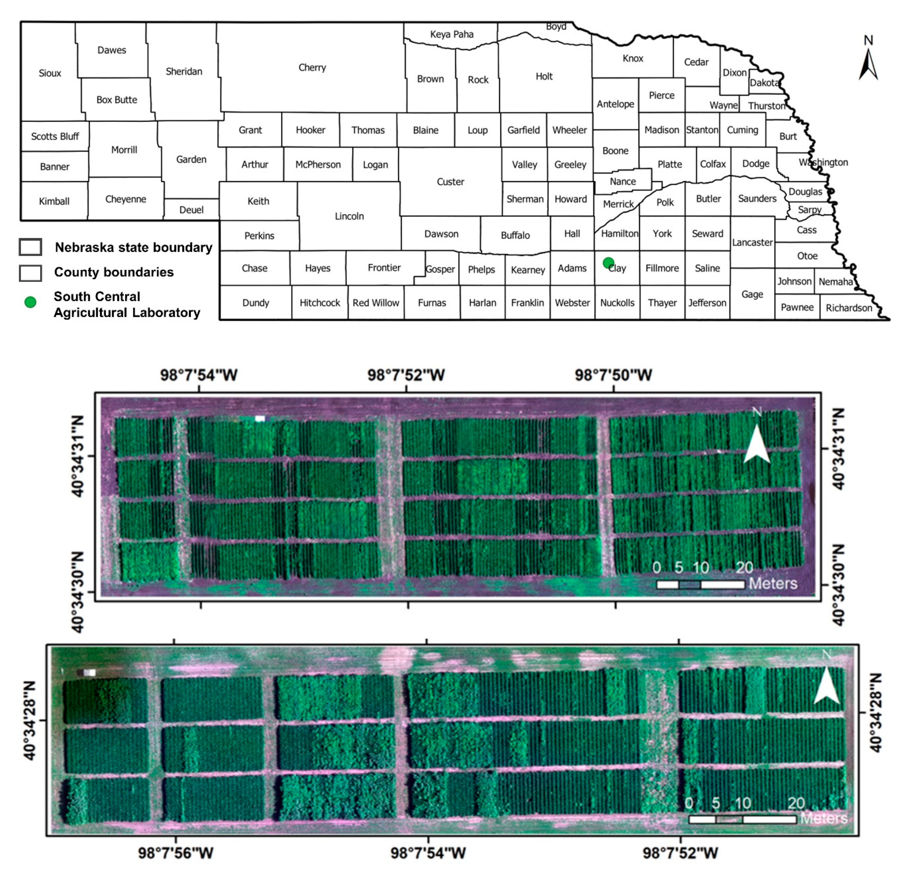
2.1. Study Site

The study sites were located in the South Central Agricultural Laboratory of the University of Nebraska, Lincoln at Clay Center, NE, USA (40.5751, -98.1309). The two study sites were located adjacent to each other. They were different soybean weed management research plots. Figure 1 shows the stitched maps of the study sites.

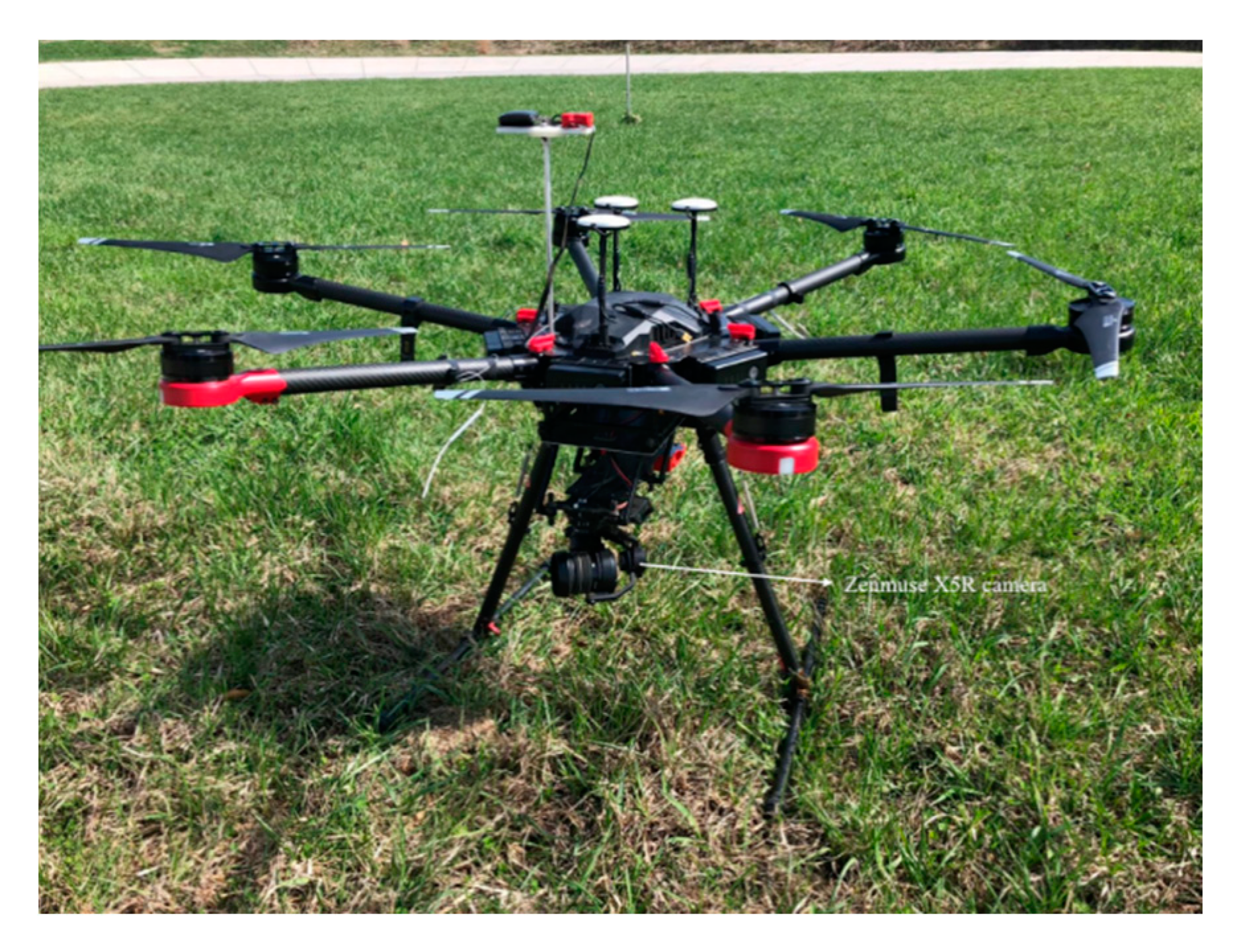
2.2. UAV Data Collection

A DJI Matrice 600 pro unmanned aerial vehicle (UAV) platform (Figure 2) was used with a Zenmuse X5R camera to capture aerial imagery. In order to collect data with varying growth stages of the crop as well as variations in illumination conditions, the images from study site 1 (shown at the top in Figure 1) were collected on 2 July 2018 whereas the images from study site 2 (shown at the bottom in Figure 1) were collected on 12 July 2018. The flight altitude in both the cases was 20m above ground level. The Zenmuse X5R camera used is a 16 megapixel camera with 4/3” sensor and 72 degree diagonal field of view. The dimension of the captured images is 4608 × 3456 pixels in three bands—Red, Green, and Blue. To develop an economical solution, this study focuses on only using RGB imagery. At a 20-m altitude, for the given sensor specifications, the spatial resolution of the output image is 0.5 cm/pixel. DJI Ground Station pro software was used for flight control. Common weed species at the experimental site were waterhemp (Amaranthus tuberculatus), Palmer amaranthus (Amaranthus palmeri), common lambsquarters (Chenopodiam album), velvetleaf (Abutilon theophrasti), and foxtail species such as yellow and green foxtails. The weeds were naturally infesting the crop and were forming patches. The two data collections were performed after 45 to 50 days after soybean planting and 15 to 20 days after post-emergence herbicides were applied in most treatments, except in plots where only pre-emergence herbicides were applied and in non-treated control plots. Soybean was at V6 (six trifoliate stage) to R2 (full flowering) growth stage.

2.3. Data Annotation and Processing

The objective of the study is to develop a weed detection system with on-farm data processing capability. Since the mosaicking of overlapping aerial images is the time-consuming process in the workflow and is not required in this case, overlapping images were removed, and only the non-overlapping raw images were retained. The original dimension of the raw image is too large to fit in the memory for processing so each raw image of size 4608 × 3456 pixels was sliced into 12 sub-images of size 1152 × 1152 pixels. The weed areas in each sub-image were annotated as rectangular bounding boxes using the python labeling tool LabelImg [53]. Only one annotator was involved in the labeling process. The annotator was trained to draw rectangular bounding boxes around weed patches. In case of weed patches of complex shapes, multiple rectangular bounding boxes were drawn to cover such patches. A total of 450 sub-images were annotated manually and were then randomly split into 90% training images and 10% test images

2.4. Patch Based CNN

Convolutional neural networks (CNNs) are feedforward artificial neural networks with the fully connected layers in the input hidden layers replaced with convolutional filters. This reduces the number of filters in each layer and enables CNNs to learn spatial patterns in images and other two-dimensional data. The advantage of a CNN is its ability to learn the features by itself, thereby preventing the need for time-consuming hand engineering of features needed in case of other Computer Vision algorithms. CNN architectures have been proposed, and its use in applications, such as document recognition by using backpropagation for training, has been studied much earlier [54]. However, their applications were limited because of the need for very large datasets to train a large number of parameters in deep networks, and also the computational needs for training. In the last decade, with advancements in parallel processing capabilities using graphical processing units and increases in the availability of large datasets, Krizhevsky et al. [36] showed the potential of CNNs in complex multiclass image classification tasks. However, in most cases, it was found that there were not enough data available to train a deep CNN from scratch. Transfer learning helped overcome this limitation. Transfer learning is the technique of using the weights of pre-trained networks trained on very large datasets such as Alexnet or GoogleNet and retraining them with small datasets for other applications [55]. This has been found to lead to exceptional classification performance and one hypothetical explanation is that the features learned in the initial convolutional layers are global features common across various image classification tasks. Several studies have looked at the application of neural networks for weed detection, such as [28,56].
In this study, a pre-trained network called Mobilenet v2 has been used for transfer learning [57]. Mobilenet v2 was developed primarily for use in mobile devices with limited memory capabilities. Hence, in order to reduce the number of parameters, each convolutional block of Mobilenet v2 consists of an expansion layer with a convolutional kernel of window size 1. This layer increases the number of channels in the input. This is followed by a depthwise convolutional layer which is then followed by a projection layer that consists of a convolutional kernel of window size 1. The depthwise convolution layer applies a single convolutional filter per input channel. The 1 × 1 convolutional layer that follows is called point wise layer. It reduces the number of channels in the output, thereby reducing the number of parameters in the next convolutional block. Hence in each block, feature maps are projected to a high dimensional space followed by learning higher dimensional features in the depthwise convolutional layer which are then encoded using a pointwise convolutional projection layer. The Mobilenet v2 network was trained on the ImageNet dataset containing 1.4 million images belonging to 1000 classes [57]. This network was then fine-tuned using the training patches belonging to both the classes in this study. Initially, for the first 10 epochs, only the classifier layer of the network were trained by freezing the weights of all other layers. This was performed to use the global features learned on the ImageNet dataset and fine-tune the classifier for this specific application. After this, fine-tuning was performed in which all the top layers were unfrozen and to allow the network to adapt to this specific application. The fine tuning was performed for 10 epochs and, hence, the model was only trained for 20 epochs in total [58].

2.5. Object Detection Models
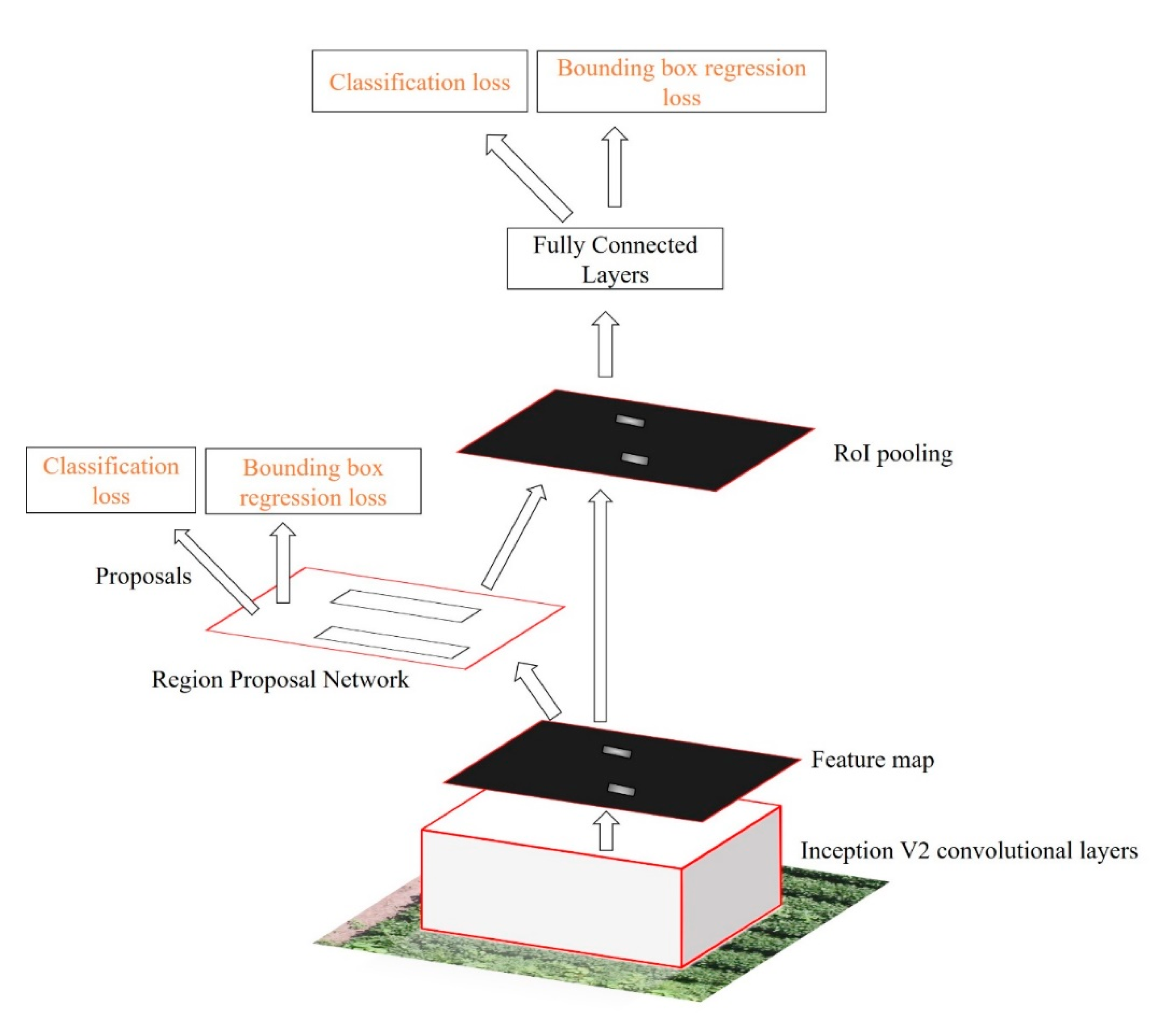
An object in Computer Vision refers to a connected, single element present in the image. Object detection is defined as the problem of finding the class of an object, and also localizing it in the image [59]. Hence, for every object in the image, the model is expected to regress the coordinates of the bounding box of the object in addition to the class probabilities for classification. Two different models have been investigated—Faster RCNN and SSD, both with Inception v2 as a feature extractor. Faster RCNN and SSD were chosen since Faster RCNN was found to have better performance, whereas SSD was found to have better speed [60]. Several different models trained on Imagenet dataset such as Inception v2 [61], Mobilenet v2 [57], Resnet 101 [62], VGG 16 [63] can be used as feature extractors for transfer learning. Of these, Inception v2 and Mobilenet v2 have been found to be the fastest in terms of inference speed [60]. The objective was to develop a weed detection system with on-farm real-time data processing capabilities. Since with similar inference speed, Inception v2 has better performance than Mobilenet v2 for object detection tasks, Inception v2 was chosen as the feature extractor [60].

2.5.1. Faster RCNN

Faster RCNN is a region proposal method-based object detection algorithm. Region-based CNN (R-CNN) was the first region proposal method-based model [64]. However, it was computationally expensive since CNN based feature extraction has to be performed for each proposed region. Fast RCNN was proposed to reduce the computational time by sharing convolutional features across the region proposals [65]. To improve the speed, Faster RCNN was proposed with fully convolutional Region Proposal Networks (RPN) that are trained to propose better object regions [66]. The Faster RCNN model consists of four sections: the feature extractor, the region proposal network, Region of Interest (RoI) pooling, and classification (as shown in Figure 3).
For feature extraction, the convolutional layers from Inception v2 were used. The advantage of the Inception v2 network is its use of wider networks with filters of different kernel sizes in each layer which makes it translation and scale invariant. Hence, the Inception v2 architecture outputs a reduced-dimensional feature map for the region proposal layer. The region proposal network is defined by anchors or fixed boundary boxes at each location. At each location, anchors of different scale and aspect ratio are defined, thereby enabling the region proposal network to make scale invariant proposals. The region proposal layer uses a convolutional filter on the feature map to output a confidence score for two classes; object and background. This is called the objectness score. Furthermore, the convolutional filter outputs regression offsets for anchor boxes. Hence, assuming there are k anchors at a location, the convolutional filter in the region proposal network outputs 6k values, namely 4k coordinates and 2k scores. Two losses are calculated from this output—classification loss and bounding box regression loss. The bounding box coordinates of anchors classified as objects are then combined with the feature map from feature extractor. In the RoI pooling layer, bounding box regions of different sizes and aspect ratios are resized to fixed size outputs using max pooling. Pooling layer refers to a down sampling layer and in case of max pooling, the down sampling is done by maximum of pixels [36]. The max-pooled feature map of a fixed size corresponding to each output is then classified, and its bounding box offsets with respect to ground truth boxes are regressed. Hence, as in the region proposal layer, two losses are computed at this output, namely the classification loss and bounding box regression loss.

2.5.2. Hyperparameters of the Architecture

In the framework that was used, the input images to the Faster RCNN network were resized to images of fixed size 1024 × 1024 pixels. At each location in the region proposal layer, 4 different scales namely 0.25, 0.5, 1.0, 2.0 and 3 different aspect ratios namely 0.5, 1.0 and 2.0 were used. Hence, in total, there were 12 anchors at each location. The model was trained for 25,000 epochs with a batch size of 1 using stochastic gradient descent with momentum optimizer. The training dataset was split into training and validation datasets and the performance of the model on validation data was continuously monitored during training to check if the model starts to overfit. Random horizontal flip and random crop operations were performed to augment the training data. The data collected had the crop rows always parallel to the horizontal axis of the image, therefore random horizontal flip and crop operations augment the training data.

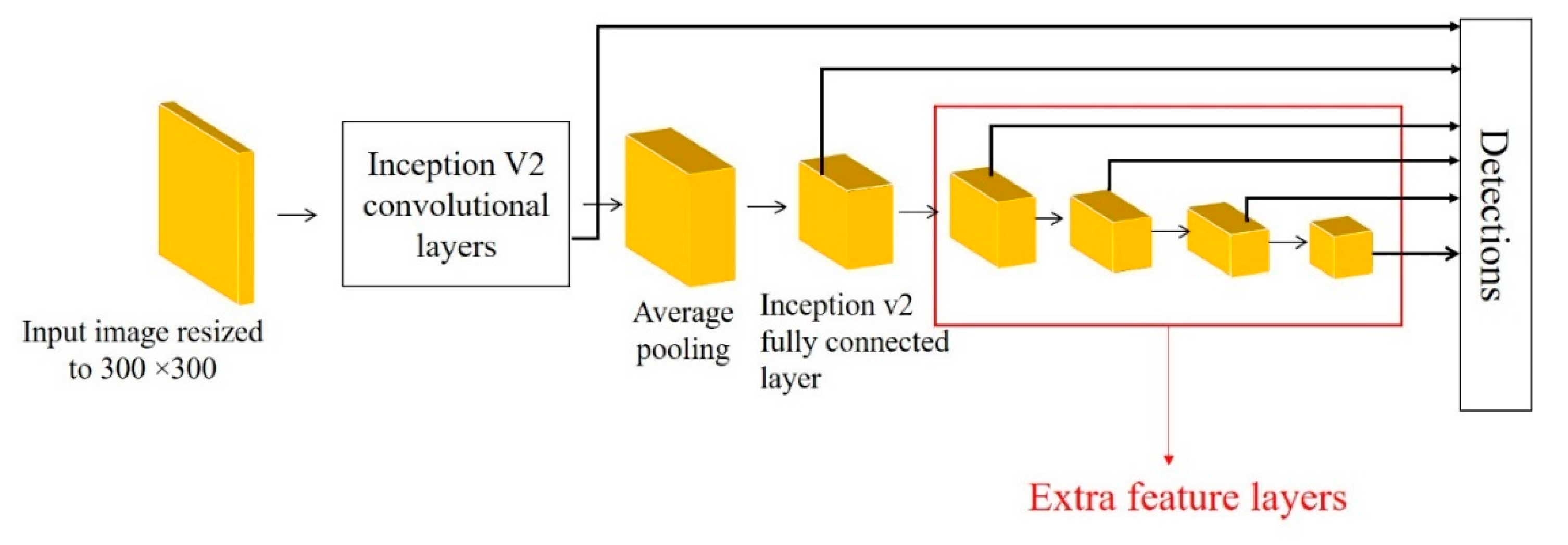
2.5.3. Single Shot Detector

The Single Shot Detector (SSD) (Figure 4) model was proposed to improve the inference time of objection detection models with region proposal network such as Faster RCNN. The main difference in SSD compared to Faster RCNN is the generation of detection outputs without a separate region proposal layer. Similar to Faster RCNN, SSD uses a feature extractor which is the Inception v2 architecture in this case. At each location of the feature map output, the model outputs a set of bounding boxes of different scales and aspect ratios. This is very similar to Faster RCNN but the difference being the convolutional filter on the feature map directly outputs the confidence scores corresponding to the output classes along with regression box offsets. Hence, the class and bounding box offsets are output in a single shot as the name suggests. For the model to be scale and translation invariant, rather than outputting bounding boxes from only the feature map, extra feature layers are added to the feature map output and detection boxes are output at different scales from each output. Hence, in total, the SSD model has 6 layers that output detection boxes at different scales [67].

2.5.4. Hyperparameters of the Architecture

In the case of SSD, in the framework that has been used, the input images are always reshaped to a fixed dimension of 300 × 300 pixels. After the feature extraction, in 6 different layers that output detection boxes, 6 different scales in the range 0.2–0.95 were used. Five different aspect ratios namely 1.0, 2.0, 0.5, 3.0 and 0.333 were generated at each location. The model was trained for 25,000 epochs as in the case of Faster RCNN. A batch size of 24 was used in training and the RMS prop optimizer was used. Data augmentation was applied with random horizontal flipping and random cropping of images. Validation images were, again, evaluated periodically during the training to check if the model is overfitting.

2.6. Hardware and Software Used

The models were trained and evaluation of the models was performed on a computer with Intel i9 processor with 18 cores and 64 GB of RAM and NVIDIA GeForce RTX 2080 Ti graphics card. Tensorflow object detection API [61] in Python was used to train and evaluate Faster RCNN and SSD. Tensorflow tutorial on transfer learning [58] was used to train the MobileNet v2 architecture for patch-based CNN.

2.7. Evaluation Metrics

Precision, recall, f1 score, and Intersection over Union (IoU) are the evaluation metrics used in this study.
Precision = TP TP + FP
Recall = TP TP + FN
F 1   score = 2 × Precision × Recall   Precision   + Recall  
Here TP refers to True Positive, FP refers to False Positive, and FN refers to False negative. Moreover, mean Average Precision (mAP) is another metric that is commonly used in object detection problems [59,68]. It is the mean of the average precision at all recall values at different IoUs for prediction and ground truth thresholds from 0.5 to 0.95. It should be noted that these metrics were primarily formulated for object detection. Even though, in this study, we use object detection models, the objective is not to find weed objects rather all the area covered by weeds for management purposes. In case of a deep learning-based object detection model, multiple objects with their bounding box are predicted. Of these, only the boxes which have IoU with the ground truth greater than threshold and class score (probability of that object being in each class) greater than confidence threshold are considered positive prediction boxes. Among these, only the box with highest class score is considered as the true positive and other positive boxes are considered as false positives. In our case, for a weed patch that is marked as a ground truth box, the model might have multiple positive weed boxes corresponding to that one ground truth box. However, only one of those would be considered as true positive and other boxes are false positives. As can be seen in the following Figure 5, the output of this image has two prediction boxes covering the weed area in the left but in the ground truth it was marked as one bounding box. Hence, if precision is used as the evaluation metric, the box on the bottom will be regarded as False Positive even though that box adds to more weed area being detected. Therefore, the Intersection over Union (IoU) of binary output image representing weed and background pixels with the ground truth binary image is used as the primary evaluation metric. The binary output images corresponding to prediction outputs and ground truth are obtained by considering pixels representing weed objects as 1 and other areas as 0. The intersection and union of the two binary images obtained are then used to find the IoU ratio. Hence, IoU here represents the ratio between the intersection of all positive prediction boxes (true positive and false positives in object detection terms) and all ground truth boxes in an image.
IoU = Area   of   overlap   Area   of   union  
To evaluate the patch-based CNN on the sub-image, an overlap slicing approach is used. The sub-image of size 1152 × 1152 pixels is sliced into patches of size 128 × 128 pixels with a stride of 32 on the horizontal and vertical. Therefore, the sliced patches have 75% horizontal and vertical overlap. Hence, each small area of size 32 × 32 is part of 8 patches and the class with maximum votes from the 4 patches is assigned as the class of the small area. To evaluate this result with ground truth and to compare with the results of Faster RCNN and SSD, IoU is used as the evaluation metric.

3. Results and Discussion

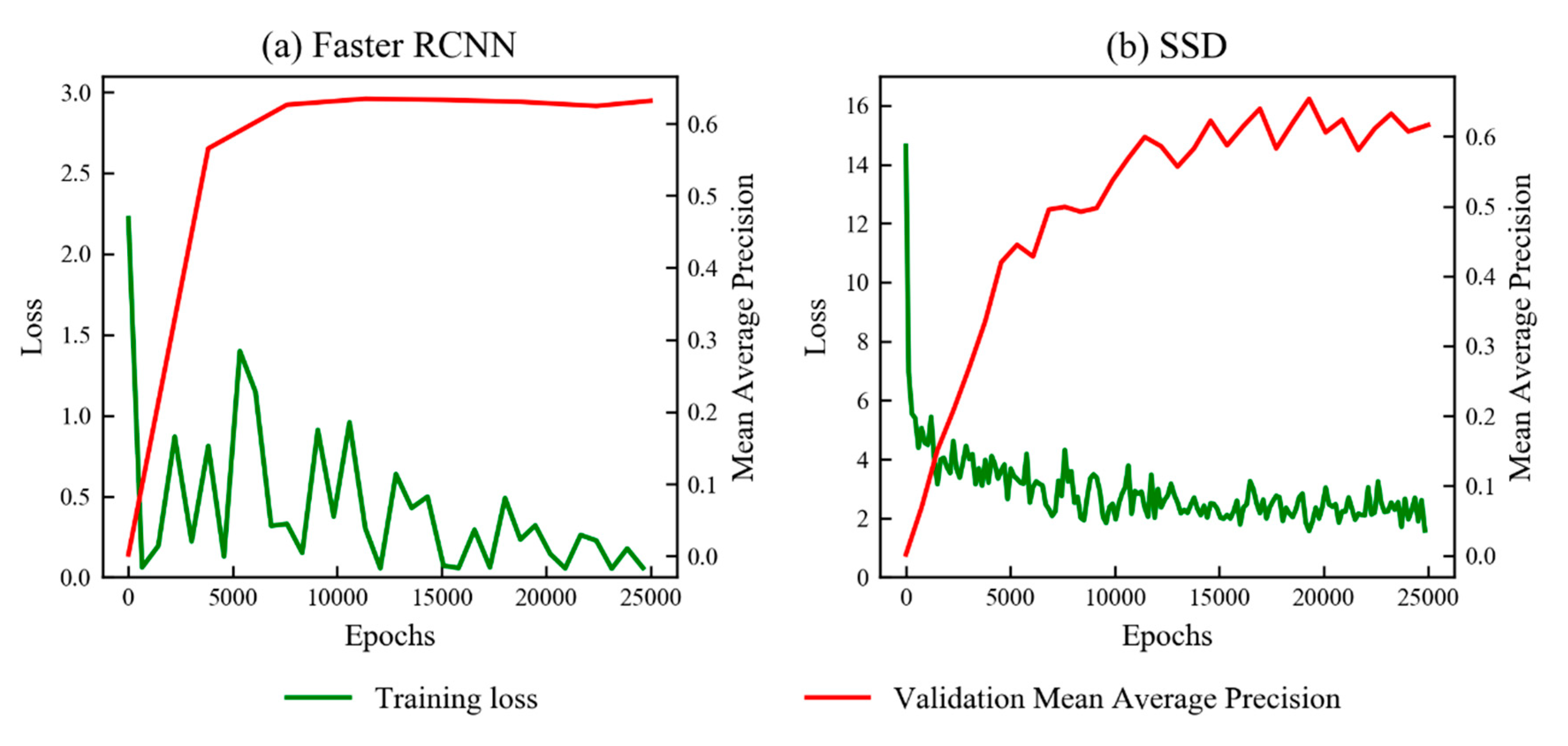
3.1. Training of Faster RCNN and SSD

Figure 6 shows the training graph for Faster RCNN and SSD. The decrease in training loss and the increase in mAP of the validation data with training epochs can be seen. By the end of the training, very little difference in the mAP of Faster RCNN and the SSD validation data was obtained. Faster RCNN converged faster than SSD. The training process of Faster RCNN might appear to oscillate more than SSD, which could be due to the different batch sizes and optimizers being used by the two models. However, it should be noted that the scale of the two loss plots was different. The different batch size and optimizer could also be the reason for the Faster RCNN model converging to high validation mAP earlier than SSD, since a batch size of 1 for Faster RCNN leads to 24 times more gradient updates than SSD with a batch size of 24.

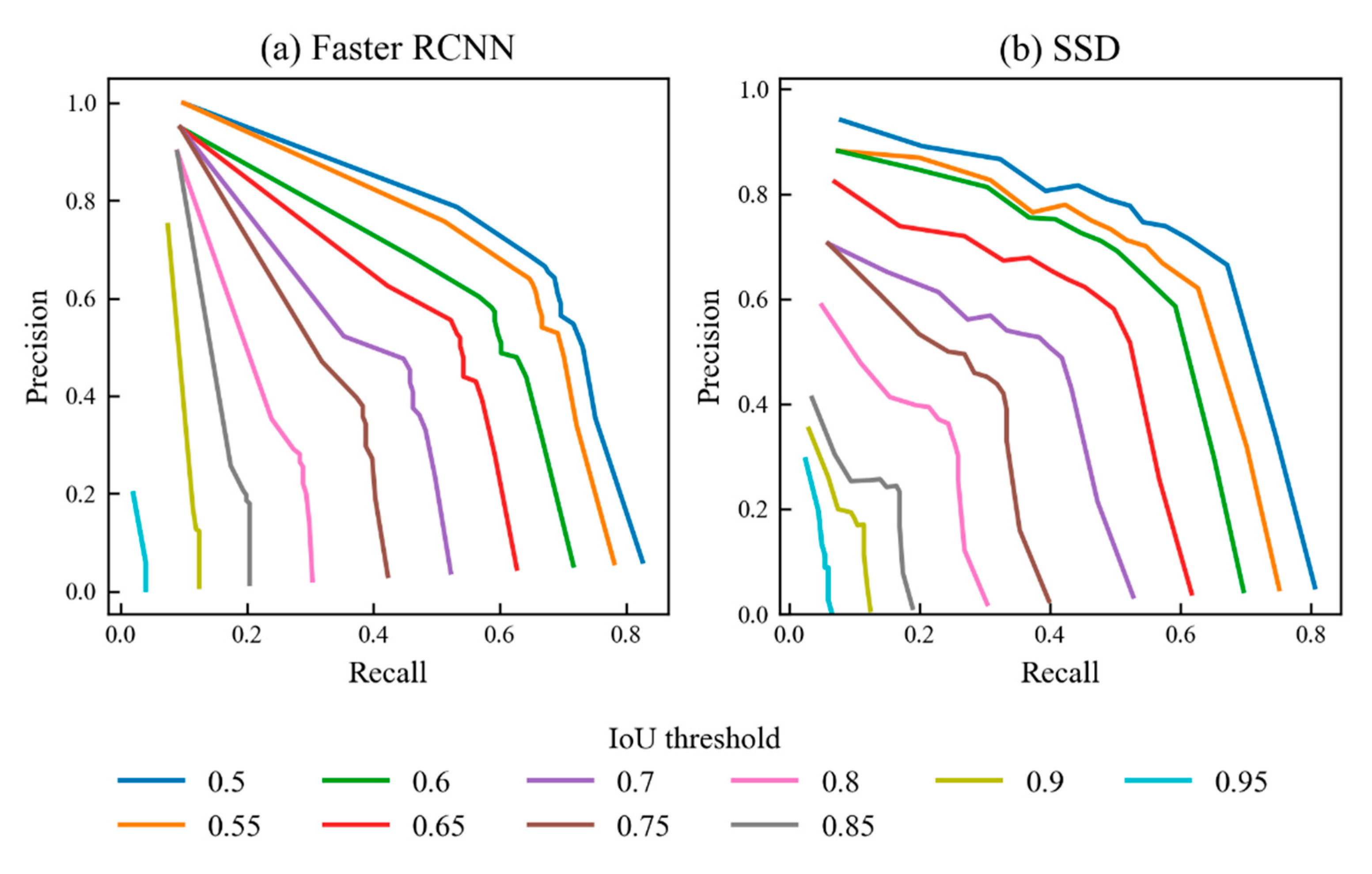
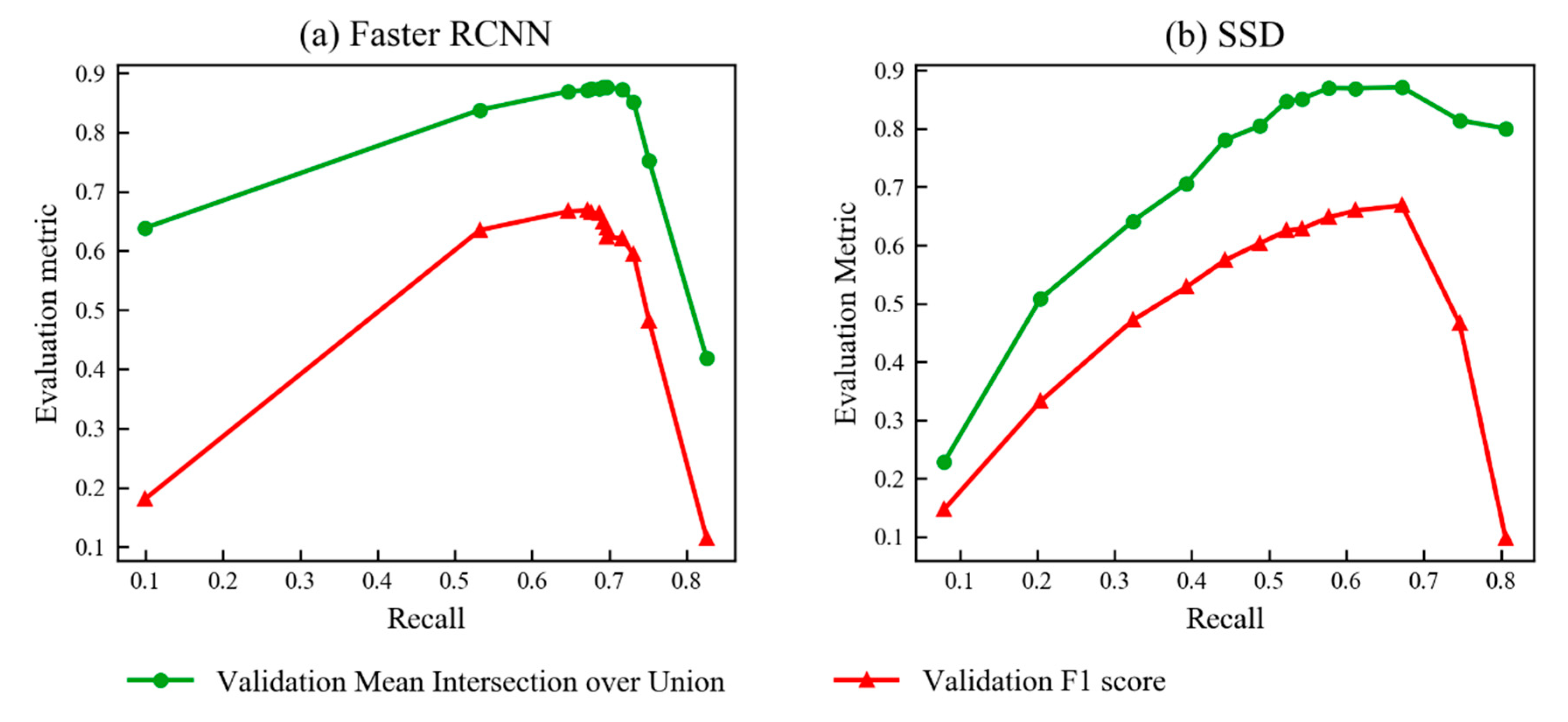
3.2. Optimal IoU and Confidence Thresholds for Faster RCNN and SSD

In order to find the optimal threshold for IoU of the prediction boxes and ground truth boxes that would result in best performance of the model, precision recall curves were drawn using various confidence thresholds from 0 to 1 at various IoU thresholds ranging from 0.5 to 0.95 (Figure 7).
It can be seen that the area under the precision-recall curve is almost the same in case of Faster RCNN and SSD which explains the fact that the validation mAP during the final epochs as seen from the training graph was very similar (0.63 in Faster RCNN and 0.62 in SSD). Furthermore, both Faster RCNN and SSD achieved the maximum area under the precision-recall curve at an IoU threshold of 0.5 for the prediction box and ground truth box. Hence, for each ground truth box, among all prediction boxes with a confidence score greater than the threshold for confidence score, the prediction box with the highest value of IoU with the ground truth box and also whose IoU with ground truth box is greater than the threshold for IoU was considered a true positive. All prediction boxes that were not a true positive with any ground truth box are regarded as false positives. The number of false negatives is equal to the number of ground truth boxes that do not have a corresponding true positive. With the optimal IoU threshold found for Faster RCNN and SSD, the following graph (Figure 8) was plotted to find the optimal confidence threshold for Faster RCNN and SSD that results in the best performance.
Figure 8 shows the change in f1 score and the mean IoU of the output binary image of the model with the ground truth binary image with change in recall. From the figure, the recall value which results in the best IoU and F1 score was found using the peak. The recall at which the best mean IoU and f1 score were observed was around 0.7 and its corresponding confidence threshold for class scores was 0.6 in the case of Faster RCNN, and 0.1 in the case of SSD. It is to be noted that mean IoU here refers to the Intersection over Union of the whole binary model output image with the ground truth binary image whereas the IoU mentioned earlier was the Intersection over Union of individual prediction bounding boxes with individual ground truth bounding boxes.

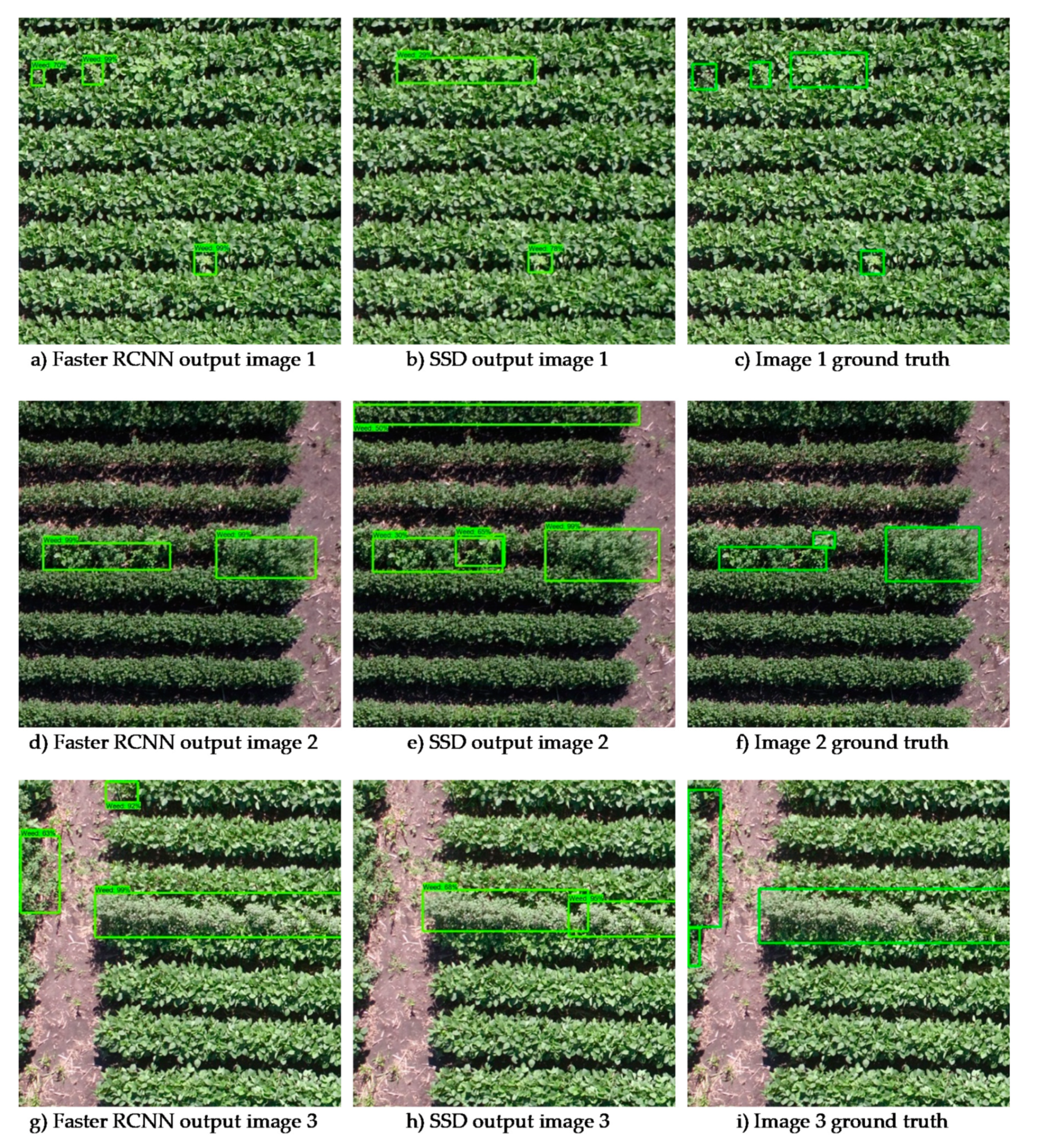
3.3. Comparison of Performance of Faster RCNN and SSD

Table 1 shows the precision, recall, f1 score, and mean IoU of the model output binary image and the ground truth binary along with the inference time for a 1152 × 1152 image. The precision, recall, f1 score, and mean IoU of both the models were similar but the SSD model was slightly faster in execution than Faster RCNN. It should be noted that the above performance was in the case that the Faster RCNN network outputs 300 proposals from the region proposal network. However, Huang et al. [36] found that by reducing the number of proposals output by Faster RCNN, the inference time of Faster RCNN can be improved with a slight cost in precision, recall, and f1 score. Therefore, experiments were conducted to study the change in inference time, precision, recall, f1 score and mean IoU, by varying the number of proposal boxes from the Faster RCNN network from 50 to 300 and the results are plotted in Figure 9.
The inference time of Faster RCNN had a linear time complexity with the number of proposal boxes output from the region proposal network. It can be seen that, from 200 to 300 proposals, there was no change in performance of the model but the inference time decreased. Hence, 200 proposals was selected as the optimal number of proposals for this dataset. At 200 proposals, the inference time of Faster RCNN was 0.21 seconds, which was the same as SSD. In the case of constraints in computational power, using 100 proposal boxes would result in significant compute savings with minimal loss in mean IoU. Hence, no difference in performance was found between Faster RCNN with 200 proposals and SSD in terms of the evaluation metrics used in this study. However, it is to be noted that, even with the same performance metric, Faster RCNN output weed objects with high confidence compared to SSD, since the confidence threshold being used for Faster RCNN was 0.6, whereas it was a very low 0.1 for SSD. Though this threshold might result in the best performance with the current validation test, it might affect the generalization performance of the model in the case of a test dataset from a different location or from a field with different management practices. In such cases, the low threshold might lead to reduced precision.
On visual observation of the outputs of all the 44 test images, it was found that in 41 images, both the networks detected all the weed areas. Hence, in these images, the difference in IoU between the model output and the ground truth is only because of the slight displacements of the boundaries of the bounding boxes from each other. As mentioned in Section 2.7, the low values of precision, recall, and f1 score obtained are primarily because of the way these metrics are calculated, since only one bounding box is considered as a true positive for one ground truth box, whereas the model in case of some weed areas with slight discontinuities outputs multiple prediction boxes to detect those areas. Therefore, the mean IoU of the binary output image with the binary image of the ground truth is the appropriate metric. In three of the test images (shown in Figure 10), there was a difference in the output of Faster RCNN and SSD. In the output image 1, Faster RCNN failed to detect a small strip of weed between the crop rows, but this was detected by SSD. However, by looking at the confidence score of the weed object from SSD, it can be understood that SSD was only able to detect this weed object because of the very low confidence threshold set for it. Whereas in output image 2, SSD misclassified a row of soybean crops with herbicide drift injury as weeds. Moreover, in case of output image 3, SSD could not detect the weeds on the left vertical border of the image. With both the failure areas being present in the border of the images, this might show the susceptibility of the SSD model in the image border. This could be due to the architecture of SSD that does detection of objects and classification into its class in a single shot, unlike Faster RCNN. Another possible reason could be that, by default, the API used to train both the models was resizing the input images of Faster RCNN to 600 × 600 whereas in case of SSD it was resized to 300 × 300. Therefore, this further loss of detail in the input image compared to the Faster RCNN input image might have led to the misclassifications in the border. Hence, further study with the same input image resolution is needed for a fair comparison.
Other than the above-mentioned three images, Faster RCNN, as well as SSD, performed exceptionally well in detecting weed objects of various scales as seen in Figure 11. As mentioned earlier, it can be seen that though SSD detected all the weed objects that were detected by Faster RCNN, the confidence of many of those predictions were very low and ended up as true positive because of the low confidence threshold. Since, by reducing the number of proposals to 200, Faster RCNN can be as fast SSD in terms of inference time, it can be concluded that Faster RCNN has better speed performance tradeoff.

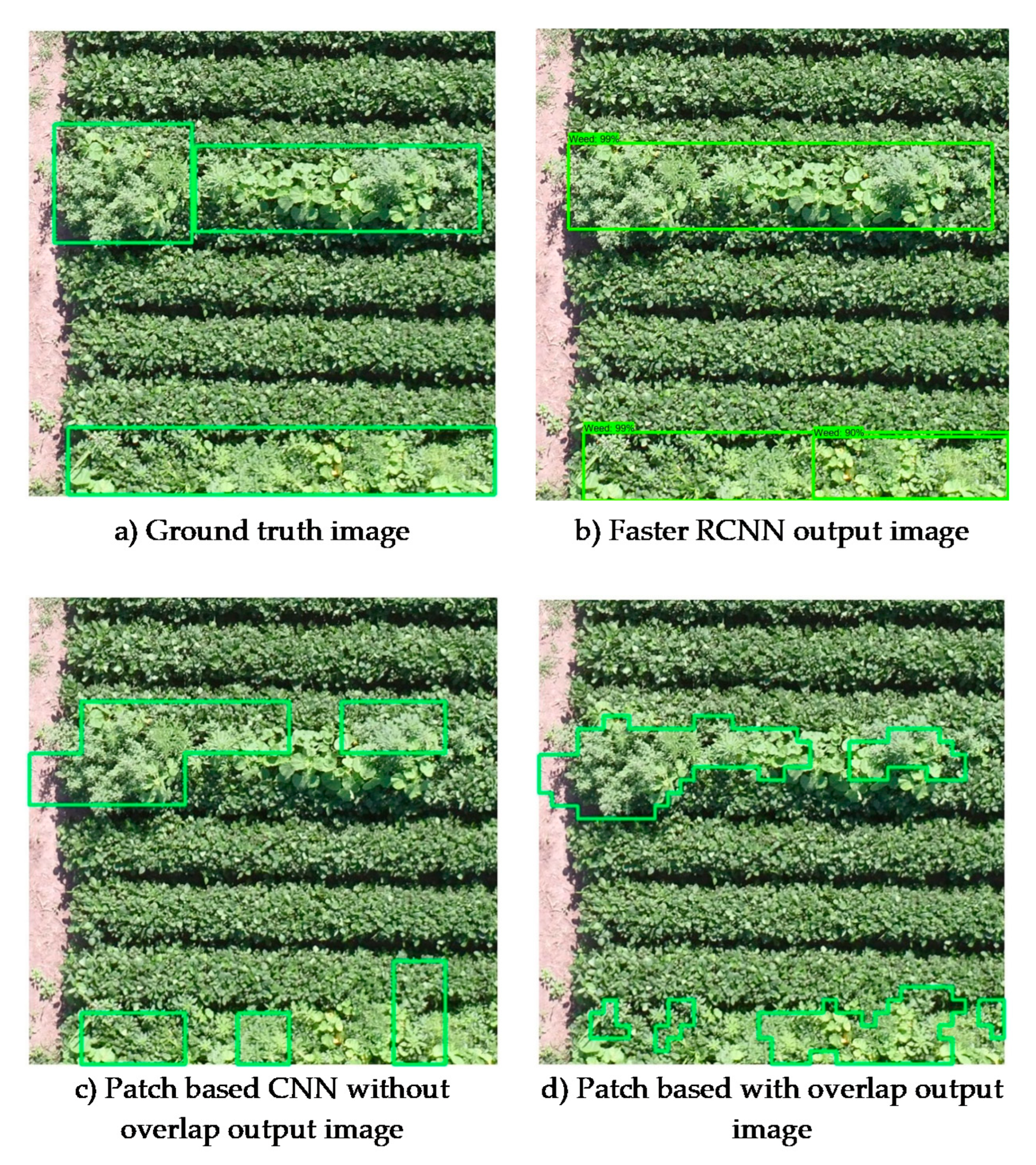
3.4. Comparison of Performance of Faster RCNN and Patch-Based CNN

The Mobilenet v2 network trained on the training patches showed very high performance in classifying test patches with an f1 score of 0.98. However, in order to evaluate its performance in detecting the weed objects in the sub-image and compare its performance with the Faster RCNN object detection model, the overlapping approach explained earlier was used. Table 2 shows the mean IoU of the output binary image from Faster RCNN and patch-based CNN with the ground truth binary image. Furthermore, the table shows the time taken to evaluate one sub-image by both the models.
Faster RCNN had better performance than patch-based CNN with overlap, both in terms of mean IoU and inference time. However, patch-based CNN without overlap has an inference time which is almost the same as Faster RCNN. The low values of IoU of patch-based CNN without overlap were because of the coarse nature of this algorithm. Since each sub-image was split into 81 patches in this approach, weeds that were smaller in size would not be detected in this approach. Furthermore, because of the way the patches were sliced, there could be a lot of patches with weeds and background in equal proportion, whereas the Mobilenet v2 model had only been trained with patches that contained only weed or only background, and hence the model was prone to error in this approach. To reduce this error, the slicing with overlap approach was tested. Since, for each small block within a patch, the class was determined by majority vote in eight patches, the problem of mixed patches was solved to some extent. Still, the similar IoU of slicing with overlap and without overlap is because the ground truth binary image represents weed objects as rectangular boxes whereas output binary images from the patch-based overlap approach consist of weed objects, which are polygonal in nature because of the majority vote as can be seen in Figure 12. Therefore, patch-based CNN with overlap has better performance than the IoU value with ground truth image suggests. However, the drawback of this approach is the very high inference time compared to Faster RCNN and patch-based RCNN without overlap. Further studies can be done with different levels of horizontal and vertical overlap and its influence on the inference time of this approach. However, with the inference time of Faster RCNN being the same as the patch-based CNN without overlap, any amount of overlap would lead to more patches to be evaluated than the non-overlap approach and hence greater inference time. Therefore, among the approaches investigated in this study, Faster RCNN had the best overall performance. It would be interesting to study a modified Fast RCNN architecture with the region proposal part replaced with an image analysis method that selects polygons. This could achieve faster computational speed as well as better performance for a patch-based CNN method.
In order to implement this system for on-farm detection, further evaluation of the performance of these approaches at higher altitudes is needed. At the altitude of 20m at which these data were collected, it is practically impossible to cover the large soybean fields with the current limitations on the battery capacity of UAV systems. Therefore, the evaluation of the performance of these models at low-resolution images from high altitude is needed for practical adoption of these systems. Like SSD, it can be seen that there is a higher misclassification rate of patches in the border of the images. In this case, it is suggested to collect images with some overlap, such as 15%, so that weed objects present in the border of one image end up in the interior of the next image. Furthermore, it is to be noted that the dataset used to train the models in the study was only collected on two different days. Therefore, the differences in phenological stage of the crop and the weed and lighting conditions are limited within the dataset. Further experiments with wide variations in lighting conditions, flight altitudes, different phenological stages are needed to analyze and compare the generalizability of performance of these models in varying conditions in the field. In addition, since the manual labeling of bounding boxes used in this study was labeled by one annotator, it is possible that there is error due to bias of the observer. Therefore, further studies using multiple annotators for labeling data with more variations as mentioned above is needed to remove bias and study the generalizability of the model. With the manual annotation of images being a time-consuming process, use of multiresolution segmentation approaches from OBIA could help in automating this. In that case, OBIA could help generate polygon labels from which rectangular bounding box labels can be generated for object detection tasks.

4. Conclusions

In this study, Faster RCNN and SSD object detection models were trained and evaluated over UAV imagery for mid- to late-season weed detection in soybean fields. The performance of two object detection models, Faster RCNN and the Single Shot Detector (SSD) models, as well as the performance of object detection CNN models with the patch-based CNN model, were evaluated and compared in terms of weed detection performance using mean IoU and inference speed.
It was found that the Faster RCNN model with 200 box proposals had a similar weed detection performance to the SSD model in terms of precision, recall, f1 score, and IoU as well as similar inference time. The precision, recall, f1 score and IoU were 0.65, 0.68, 0.66 and 0.85 for Faster RCNN with 200 proposals, and 0.66, 0.68, 0.67 and 0.84 for SSD respectively. However, the optimal confidence threshold of SSD was found to be 0.1, indicating the lower confidence of this model in the case of weed objects detected, whereas the optimal confidence threshold was found to be 0.6 in the case of Faster RCNN, meaning higher confidence in the weed objects detected. In addition, SSD was susceptible to misclassification in the border of some test images. These findings indicate that SSD might have lower generalization performance than Faster RCNN for mid- to late-season weed detection in soybean fields using UAV imagery. Hence, Faster RCNN was determined to be the better performing model among the two in this study. Between Faster RCNN and patch-based CNN, Faster RCNN had better weed detection performance than patch-based CNN with overlap as well as without overlap. The inference time of Faster RCNN was similar to patch-based CNN without overlap, but significantly less than patch-based CNN with overlap. Hence, Faster RCNN was found to be the best model in terms of weed detection performance and inference time among the different models compared in this study.
Future work can evaluate the performance variation of models in different weed species. In addition, the performance of Faster RCNN at different altitudes by resampling high-resolution images to low-resolution images can be studied. Furthermore, the inference time experiments at different altitudes should be performed on low computational power devices such as regular laptops and mini-PCs used for the flight control of UAV systems. Inference time experiments should also be performed on low cost hardware accelerators available for edge computing such as the Intel Neural Compute Stick or Google Coral. This would help understand the potential of using such devices for on-farm, near real-time data processing and actuation. In addition, the effect of model compression techniques and approximation algorithms developed for neural networks can be studied to understand the limit of edge computing for in-field near real-time weed detection. Moreover, further work can be performed on using the RTK GPS data of individual images and their corresponding IMU data to orthorectify the image and find the geolocation of the weed patches detected by the object detection models. In addition, the performance of object detection models for weed detection can be compared between raw individual images as used in this study and stitched mosaic maps. With the manual annotation of images being a laborious part of the process, using techniques such as self-supervised learning [69] and active learning [70] to reduce the amount of manual labeling for this task can be studied. Furthermore, few-shot learning algorithms can be studied to investigate the transfer learning of this algorithm to other crops and weed species by training with a few labeled instances from those crops and weed species.

Author Contributions

Conceptualization, Y.S. and E.P.; methodology, A.N.V.S., Y.S. and S.S.; data acquisition, A.N.V.S. and J.L.; software, analysis and evaluation, A.N.V.S.; writing—original draft preparation, A.N.V.S.; writing—review and editing, Y.S., E.P., S.S., A.J.J., J.D.L. and J.L.; project administration, Y.S.; funding acquisition, Y.S., E.P. and A.J.J. All authors have read and agreed to the published version of the manuscript.

Funding

This research was funded by the Nebraska Research Initiative (NRI) Collaboration Initiative Seed Grant 2132250011, the Nebraska Corn Board, and the Nebraska Agricultural Experiment Station through the Hatch Act capacity funding program (Accession Number 1011130) from the USDA National Institute of Food and Agriculture.

Acknowledgments

Thanks to Jonathan Forbes for their assistance in data collection.

Conflicts of Interest

The authors declare no conflict of interest. The funders had no role in the design of the study; in the collection, analyses, or interpretation of data; in the writing of the manuscript, or in the decision to publish the results.

References

  1. Dos Santos Ferreira, A.; Matte Freitas, D.; Gonçalves da Silva, G.; Pistori, H.; Theophilo Folhes, M. Weed detection in soybean crops using ConvNets. Comput. Electron. Agric. 2017, 143, 314–324. [Google Scholar] [CrossRef]
  2. Thorp, K.R.; Tian, L.F. A Review on Remote Sensing of Weeds in Agriculture. Precis. Agric. 2004, 5, 477–508. [Google Scholar] [CrossRef]
  3. Weis, M.; Gutjahr, C.; Rueda Ayala, V.; Gerhards, R.; Ritter, C.; Schölderle, F. Precision farming for weed management: Techniques. Gesunde Pflanz. 2008, 60, 171–181. [Google Scholar] [CrossRef]
  4. Christensen, S.; SØgaard, H.T.; Kudsk, P.; NØrremark, M.; Lund, I.; Nadimi, E.S.; JØrgensen, R. Site-specific weed control technologies. Weed Res. 2009. [Google Scholar] [CrossRef]
  5. Zhang, N.; Wang, M.; Wang, N. Precision agriculture—A worldwide overview. Comput. Electron. Agric. 2002, 36, 113–132. [Google Scholar] [CrossRef]
  6. O’Donovan, J.T.; De St. Remy, E.A.; O’Sullivan, P.A.; Dew, D.A.; Sharma, A.K. Influence of the Relative Time of Emergence of Wild Oat ( Avena fatua ) on Yield Loss of Barley ( Hordeum vulgare ) and Wheat ( Triticum aestivum). Weed Sci. 1985. [Google Scholar] [CrossRef]
  7. Swanton, C.J.; Mahoney, K.J.; Chandler, K.; Gulden, R.H. Integrated Weed Management: Knowledge-Based Weed Management Systems. Weed Sci. 2008. [Google Scholar] [CrossRef]
  8. JUDGE, C.A.; NEAL, J.C.; DERR, J.F. Response of Japanese Stiltgrass (Microstegium vimineum) to Application Timing, Rate, and Frequency of Postemergence Herbicides 1. Weed Technol. 2005. [Google Scholar] [CrossRef]
  9. Chauhan, B.S.; Singh, R.G.; Mahajan, G. Ecology and management of weeds under conservation agriculture: A review. Crop. Prot. 2012, 38, 57–65. [Google Scholar] [CrossRef]
  10. De Castro, A.I.; Torres-Sánchez, J.; Peña, J.M.; Jiménez-Brenes, F.M.; Csillik, O.; López-Granados, F. An automatic random forest-OBIA algorithm for early weed mapping between and within crop rows using UAV imagery. Remote Sens. 2018, 10, 285. [Google Scholar] [CrossRef] [Green Version]
  11. Fernández-Quintanilla, C.; Peña, J.M.; Andújar, D.; Dorado, J.; Ribeiro, A.; López-Granados, F. Is the current state of the art of weed monitoring suitable for site-specific weed management in arable crops? Weed Res. 2018, 58, 259–272. [Google Scholar] [CrossRef]
  12. López-Granados, F. Weed detection for site-specific weed management: Mapping and real-time approaches. Weed Res. 2011. [Google Scholar] [CrossRef] [Green Version]
  13. Barroso, J.; Fernàndez-Quintanilla, C.; Ruiz, D.; Hernaiz, P.; Rew, L.J. Spatial stability of Avena sterilis ssp. ludoviciana populations under annual applications of low rates of imazamethabenz. Weed Res. 2004. [Google Scholar] [CrossRef]
  14. Koger, C.H.; Shaw, D.R.; Watson, C.E.; Reddy, K.N. Detecting Late-Season Weed Infestations in Soybean (Glycine max) 1. Weed Technol. 2003. [Google Scholar] [CrossRef]
  15. De Castro, A.I.; Jurado-Expósito, M.; Peña-Barragán, J.M.; López-Granados, F. Airborne multi-spectral imagery for mapping cruciferous weeds in cereal and legume crops. Precis. Agric. 2012. [Google Scholar] [CrossRef] [Green Version]
  16. De Castro, A.I.; López-Granados, F.; Jurado-Expósito, M. Broad-scale cruciferous weed patch classification in winter wheat using QuickBird imagery for in-season site-specific control. Precis. Agric. 2013. [Google Scholar] [CrossRef] [Green Version]
  17. Castillejo-González, I.L.; López-Granados, F.; García-Ferrer, A.; Peña-Barragán, J.M.; Jurado-Expósito, M.; de la Orden, M.S.; González-Audicana, M. Object- and pixel-based analysis for mapping crops and their agro-environmental associated measures using QuickBird imagery. Comput. Electron. Agric. 2009. [Google Scholar] [CrossRef]
  18. Meyer, G.E.; Mehta, T.; Kocher, M.F.; Mortensen, D.A.; Samal, A. Textural imaging and discriminant analysis for distinguishing weeds for spot spraying. Trans. Am. Soc. Agric. Eng. 1998. [Google Scholar] [CrossRef]
  19. Burks, T.F.; Shearer, S.A.; Payne, F.A. Classification of weed species using color texture features and discriminant analysis. Trans. Am. Soc. Agric. Eng. 2000, 43, 411. [Google Scholar] [CrossRef]
  20. Wang, A.; Zhang, W.; Wei, X. A review on weed detection using ground-based machine vision and image processing techniques. Comput. Electron. Agric. 2019, 158, 226–240. [Google Scholar] [CrossRef]
  21. Sankaran, S.; Khot, L.R.; Espinoza, C.Z.; Jarolmasjed, S.; Sathuvalli, V.R.; Vandemark, G.J.; Miklas, P.N.; Carter, A.H.; Pumphrey, M.O.; Knowles, N.R.; et al. Low-altitude, high-resolution aerial imaging systems for row and field crop phenotyping: A review. Eur. J. Agron. 2015, 70, 112–123. [Google Scholar] [CrossRef]
  22. Rasmussen, J.; Nielsen, J.; Streibig, J.C.; Jensen, J.E.; Pedersen, K.S.; Olsen, S.I. Pre-harvest weed mapping of Cirsium arvense in wheat and barley with off-the-shelf UAVs. Precis. Agric. 2019. [Google Scholar] [CrossRef]
  23. Casa, R.; Pascucci, S.; Pignatti, S.; Palombo, A.; Nanni, U.; Harfouche, A.; Laura, L.; Di Rocco, M.; Fantozzi, P. UAV-based hyperspectral imaging for weed discrimination in maize. In Proceedings of the Precision Agriculture 2019—Papers Presented at the 12th European Conference on Precision Agriculture, ECPA 2019, Montpellier, France, 8–11 July 2019; Wageningen Academic Publishers: Wageningen, The Netherlands, 2019; pp. 365–371. [Google Scholar]
  24. Sánchez-Sastre, L.F.; Casterad, M.A.; Guillén, M.; Ruiz-Potosme, N.M.; Veiga, N.M.S.A.; da Navas-Gracia, L.M.; Martín-Ramos, P. UAV Detection of Sinapis arvensis Infestation in Alfalfa Plots Using Simple Vegetation Indices from Conventional Digital Cameras. AgriEngineering 2020, 2, 12. [Google Scholar] [CrossRef] [Green Version]
  25. Peña-Barragán, J.M.; López-Granados, F.; Jurado-Expósito, M.; García-Torres, L. Spectral discrimination of Ridolfia segetum and sunflower as affected by phenological stage. Weed Res. 2006. [Google Scholar] [CrossRef]
  26. Gray, C.J.; Shaw, D.R.; Gerard, P.D.; Bruce, L.M. Utility of Multispectral Imagery for Soybean and Weed Species Differentiation. Weed Technol. 2008. [Google Scholar] [CrossRef]
  27. Martin, M.P.; Barreto, L.; RiañO, D.; Fernandez-Quintanilla, C.; Vaughan, P. Assessing the potential of hyperspectral remote sensing for the discrimination of grassweeds in winter cereal crops. Int. J. Remote Sens. 2011. [Google Scholar] [CrossRef]
  28. De Castro, A.I.; Jurado-Expósito, M.; Gómez-Casero, M.T.; López-Granados, F. Applying neural networks to hyperspectral and multispectral field data for discrimination of cruciferous weeds in winter crops. Sci. World J. 2012. [Google Scholar] [CrossRef] [Green Version]
  29. Peña, J.M.; Torres-Sánchez, J.; de Castro, A.I.; Kelly, M.; López-Granados, F. Weed Mapping in Early-Season Maize Fields Using Object-Based Analysis of Unmanned Aerial Vehicle (UAV) Images. PLoS ONE 2013, 8, e77151. [Google Scholar] [CrossRef] [Green Version]
  30. Torres-Sánchez, J.; López-Granados, F.; De Castro, A.I.; Peña-Barragán, J.M. Configuration and Specifications of an Unmanned Aerial Vehicle (UAV) for Early Site Specific Weed Management. PLoS ONE 2013, 8, e58210. [Google Scholar] [CrossRef] [Green Version]
  31. Torres-Sánchez, J.; Peña, J.M.; de Castro, A.I.; López-Granados, F. Multi-temporal mapping of the vegetation fraction in early-season wheat fields using images from UAV. Comput. Electron. Agric. 2014. [Google Scholar] [CrossRef]
  32. Pérez-Ortiz, M.; Peña, J.M.; Gutiérrez, P.A.; Torres-Sánchez, J.; Hervás-Martínez, C.; López-Granados, F. A semi-supervised system for weed mapping in sunflower crops using unmanned aerial vehicles and a crop row detection method. Appl. Soft Comput. 2015, 37, 533–544. [Google Scholar] [CrossRef]
  33. Castaldi, F.; Pelosi, F.; Pascucci, S.; Casa, R. Assessing the potential of images from unmanned aerial vehicles (UAV) to support herbicide patch spraying in maize. Precis. Agric. 2017. [Google Scholar] [CrossRef]
  34. López-Granados, F.; Torres-Sánchez, J.; Serrano-Pérez, A.; de Castro, A.I.; Mesas-Carrascosa, F.-J.; Peña, J.-M. Early season weed mapping in sunflower using UAV technology: Variability of herbicide treatment maps against weed thresholds. Precis. Agric. 2016, 17, 183–199. [Google Scholar] [CrossRef]
  35. Liu, D.; Xia, F. Assessing object-based classification: Advantages and limitations Assessing object-based classification: Advantages and limitations. Remote Sens. Lett. 2010. [Google Scholar] [CrossRef]
  36. Krizhevsky, A.; Sutskever, I.; Hinton, G.E. ImageNet classification with deep convolutional neural networks. In Proceedings of the Advances in Neural Information Processing Systems, Lake Tahoe, NV, USA, 3–6 December 2012; pp. 1097–1105. [Google Scholar]
  37. Steen, K.; Christiansen, P.; Karstoft, H.; Jørgensen, R.; Steen, K.A.; Christiansen, P.; Karstoft, H.; Jørgensen, R.N. Using Deep Learning to Challenge Safety Standard for Highly Autonomous Machines in Agriculture. J. Imaging 2016, 2, 6. [Google Scholar] [CrossRef] [Green Version]
  38. Song, X.; Zhang, G.; Liu, F.; Li, D.; Zhao, Y.; Yang, J. Modeling spatio-temporal distribution of soil moisture by deep learning-based cellular automata model. J. Arid Land 2016, 8, 734–748. [Google Scholar] [CrossRef] [Green Version]
  39. Mohanty, S.P.; Hughes, D.P.; Salathé, M. Using Deep Learning for Image-Based Plant Disease Detection. Front. Plant. Sci. 2016, 7, 1419. [Google Scholar] [CrossRef] [Green Version]
  40. Kuwata, K.; Shibasaki, R. Estimating crop yields with deep learning and remotely sensed data. In Proceedings of the 2015 IEEE International Geoscience and Remote Sensing Symposium (IGARSS), Milan, Italy, 26–31 July 2015; pp. 858–861. [Google Scholar]
  41. Rahnemoonfar, M.; Sheppard, C.; Rahnemoonfar, M.; Sheppard, C. Deep Count: Fruit Counting Based on Deep Simulated Learning. Sensors 2017, 17, 905. [Google Scholar] [CrossRef] [Green Version]
  42. Andrea, C.-C.; Mauricio Daniel, B.B.; Jose Misael, J.B. Precise weed and maize classification through convolutional neuronal networks. In Proceedings of the 2017 IEEE Second Ecuador Technical Chapters Meeting (ETCM), Salinas, Ecuador, 16–20 October 2017; pp. 1–6. [Google Scholar]
  43. Dyrmann, M.; Mortensen, A.; Midtiby, H.; Jørgensen, R. Pixel-wise classification of weeds and crops in images by using a fully convolutional neural network. In Proceedings of the International Conference on Agricultural Engineering, Aarhus, Denmark, 26–29 June 2016; pp. 26–29. [Google Scholar]
  44. Milioto, A.; Lottes, P.; Stachniss, C. Real-Time Semantic Segmentation of Crop and Weed for Precision Agriculture Robots Leveraging Background Knowledge in CNNs. In Proceedings of the 2018 IEEE International Conference on Robotics and Automation (ICRA), Brisbane, Australia, 21–25 May 2018; pp. 2229–2235. [Google Scholar]
  45. Lottes, P.; Behley, J.; Milioto, A.; Stachniss, C. Fully Convolutional Networks With Sequential Information for Robust Crop and Weed Detection in Precision Farming. IEEE Robot. Autom. Lett. 2018, 3, 2870–2877. [Google Scholar] [CrossRef] [Green Version]
  46. Lottes, P.; Khanna, R.; Pfeifer, J.; Siegwart, R.; Stachniss, C. UAV-based crop and weed classification for smart farming. In Proceedings of the 2017 IEEE International Conference on Robotics and Automation (ICRA), Singapore, 29 May–3 June 2017; pp. 3024–3031. [Google Scholar]
  47. Lottes, P.; Behley, J.; Chebrolu, N.; Milioto, A.; Stachniss, C. Robust joint stem detection and crop-weed classification using image sequences for plant-specific treatment in precision farming. J. Field Robot. 2020, 37, 20–34. [Google Scholar] [CrossRef]
  48. Sa, I.; Chen, Z.; Popovic, M.; Khanna, R.; Liebisch, F.; Nieto, J.; Siegwart, R. WeedNet: Dense Semantic Weed Classification Using Multispectral Images and MAV for Smart Farming. IEEE Robot. Autom. Lett. 2018, 3, 588–595. [Google Scholar] [CrossRef] [Green Version]
  49. Sa, I.; Popović, M.; Khanna, R.; Chen, Z.; Lottes, P.; Liebisch, F.; Nieto, J.; Stachniss, C.; Walter, A.; Siegwart, R.; et al. WeedMap: A Large-Scale Semantic Weed Mapping Framework Using Aerial Multispectral Imaging and Deep Neural Network for Precision Farming. Remote Sens. 2018, 10, 1423. [Google Scholar] [CrossRef] [Green Version]
  50. Bah, M.D.; Dericquebourg, E.; Hafiane, A.; Canals, R. Deep Learning Based Classification System for Identifying Weeds Using High-Resolution UAV Imagery. In Intelligent Computing. SAI 2018; Advances in Intelligent Systems and Computing: Cham, Switzerland, 2019; Volume 857, pp. 176–187. [Google Scholar]
  51. Huang, H.; Deng, J.; Lan, Y.; Yang, A.; Deng, X.; Zhang, L. A fully convolutional network for weed mapping of unmanned aerial vehicle (UAV) imagery. PLoS ONE 2018, 13, e0196302. [Google Scholar] [CrossRef] [Green Version]
  52. Yu, J.; Schumann, A.W.; Cao, Z.; Sharpe, S.M.; Boyd, N.S. Weed Detection in Perennial Ryegrass With Deep Learning Convolutional Neural Network. Front. Plant Sci. 2019, 10. [Google Scholar] [CrossRef] [PubMed] [Green Version]
  53. Tzutalin LabelImg. LabelImg 2015. Available online: https://github.com/tzutalin/labelImg (accessed on 30 June 2020).
  54. LeCun, Y.; Bottou, L.; Bengio, Y.; Haffner, P. Gradient-based learning applied to document recognition. Proc. IEEE 1998, 86, 2278–2324. [Google Scholar] [CrossRef] [Green Version]
  55. Torrey, L.; Shavlik, J. Transfer learning. In Handbook of Research on Machine Learning Applications and Trends: Algorithms, Methods, and Techniques; IGI Global: Hershey, PA, USA, 2010; pp. 242–264. [Google Scholar]
  56. Karimi, Y.; Prasher, S.O.; McNairn, H.; Bonnell, R.B.; Dutilleul, P.; Goel, P.K. Classification accuracy of discriminant analysis, artificial neural networks, and decision trees for weed and nitrogen stress detection in corn. Trans. Am. Soc. Agric. Eng. 2005. [Google Scholar] [CrossRef]
  57. Sandler, M.; Howard, A.; Zhu, M.; Zhmoginov, A.; Chen, L.C. MobileNetV2: Inverted Residuals and Linear Bottlenecks. In Proceedings of the IEEE Computer Society Conference on Computer Vision and Pattern Recognition, Salt Lake City, UT, USA, 18–23 June 2018; pp. 4510–4520. [Google Scholar]
  58. Chollet, F. Transfer Learning Using Pretrained ConvNets. Available online: https://www.tensorflow.org/alpha/tutorials/images/transfer_learning (accessed on 30 June 2020).
  59. Lin, T.Y.; Maire, M.; Belongie, S.; Hays, J.; Perona, P.; Ramanan, D.; Dollár, P.; Zitnick, C.L. Microsoft COCO: Common objects in context. In Computer Vision—ECCV 2014; Lecture Notes in Computer Science: Cham, Switzerland, 2014; pp. 740–755. [Google Scholar] [CrossRef] [Green Version]
  60. Huang, J.; Rathod, V.; Sun, C.; Zhu, M.; Korattikara, A.; Fathi, A.; Murphy, K. Speed/accuracy trade-offs for modern convolutional object detectors. In Proceedings of the IEEE Conference on Computer Vision and Pattern Recognition, Honolulu, HI, USA, 21–26 July 2017; pp. 7310–7311. [Google Scholar]
  61. Szegedy, C.; Vanhoucke, V.; Ioffe, S.; Shlens, J.; Wojna, Z. Rethinking the Inception Architecture for Computer Vision. In Proceedings of the IEEE Computer Society Conference on Computer Vision and Pattern Recognition, Las Vegas, NV, USA, 27–30 June 2016; Volume 2016, pp. 2818–2826. [Google Scholar]
  62. He, K.; Zhang, X.; Ren, S.; Sun, J. Deep residual learning for image recognition. In Proceedings of the IEEE Computer Society Conference on Computer Vision and Pattern Recognition, Las Vegas, NV, USA, 27–30 June 2016; Volume 2016, pp. 770–778. [Google Scholar]
  63. Liu, S.; Deng, W. Very deep convolutional neural network based image classification using small training sample size. In Proceedings of the 3rd IAPR Asian Conference on Pattern Recognition, ACPR 2015, Kuala Lumpur, Malaysia, 3–6 November 2015; pp. 730–734. [Google Scholar]
  64. Girshick, R.; Donahue, J.; Darrell, T.; Malik, J. Region-Based Convolutional Networks for Accurate Object Detection and Segmentation. IEEE Trans. Pattern Anal. Mach. Intell. 2016, 38, 142–158. [Google Scholar] [CrossRef]
  65. Girshick, R. Fast R-CNN. In Proceedings of the IEEE International Conference on Computer Vision, Santiago, Chile, 7–13 December 2015. [Google Scholar]
  66. Ren, S.; He, K.; Girshick, R.; Sun, J. Faster R-CNN: Towards Real-Time Object Detection with Region Proposal Networks. IEEE Trans. Pattern Anal. Mach. Intell. 2017, 39, 1137–1149. [Google Scholar] [CrossRef] [Green Version]
  67. Liu, W.; Anguelov, D.; Erhan, D.; Szegedy, C.; Reed, S.; Fu, C.-Y.; Berg, A.C. SSD: Single Shot MultiBox Detector. In Computer Vision—ECCV 2016; Lecture Notes in Computer Science: Cham, Switzerland, 2015. [Google Scholar] [CrossRef] [Green Version]
  68. Everingham, M.; Van Gool, L.; Williams, C.K.I.; Winn, J.; Zisserman, A. The pascal visual object classes (VOC) challenge. Int. J. Comput. Vis. 2010, 88, 303–338. [Google Scholar] [CrossRef] [Green Version]
  69. Doersch, C.; Gupta, A.; Efros, A.A. Unsupervised visual representation learning by context prediction. In Proceedings of the IEEE International Conference on Computer Vision, Santiago, Chile, 7–13 December 2015. [Google Scholar]
  70. Brust, C.A.; Käding, C.; Denzler, J. Active learning for deep object detection. In Proceedings of the VISIGRAPP 2019—14th International Joint Conference on Computer Vision, Imaging and Computer Graphics Theory and Applications, Prague, Czech, 25–27 February 2019; SciTePress: Setúbal, Portugal, 2019; Volume 5, pp. 181–190. [Google Scholar]
Figure 1. Study area at South Central Ag Laboratory in Clay Center, NE.
Remotesensing 12 02136 g001
Figure 2. DJI Matrice 600 pro UAV platform with Zenmuse X5R camera.
Remotesensing 12 02136 g002
Figure 3. Faster RCNN architecture.
Remotesensing 12 02136 g003
Figure 4. Single Shot Detector (SSD) architecture.
Remotesensing 12 02136 g004
Figure 5. Example output image showing a weed patch annotated with single box in ground truth image detected as two boxes in output. This will lead to lesser precision as only the bigger box is considered true positive and therefore IoU is a better evaluation metric for this problem.
Remotesensing 12 02136 g005
Figure 6. Change in training loss and Validation Mean Average Precision with number of epochs of (a) Faster RCNN and (b) SSD.
Remotesensing 12 02136 g006
Figure 7. Precision-recall curve at different thresholds for IoU of the predicted box and ground truth box (a) Faster RCNN and (b) SSD.
Remotesensing 12 02136 g007
Figure 8. Change in IoU of output binary image and ground truth binary image as well as f1 score with change in recall.
Remotesensing 12 02136 g008
Figure 9. Change in evaluation metrics and inference time of Faster RCNN model with increase in number of proposals.
Remotesensing 12 02136 g009
Figure 10. Output images with discrepancies between Faster RCNN and SSD and their corresponding ground truth.
Remotesensing 12 02136 g010
Figure 11. Example output images with good model performance.
Remotesensing 12 02136 g011
Figure 12. Output images of patch-based CNN and Faster RCNN.
Remotesensing 12 02136 g012
Table 1. Performance of test data in Faster RCNN and Single Shot Detector (SSD).
ModelPrecisionRecallF1 ScoreMean IoUInference Time of 1152 × 1152 Image in Seconds
Faster RCNN0.650.680.660.850.23
SSD0.660.680.670.840.21
Table 2. Performance of Faster RCNN and patch-based CNN in test sub-images.
ModelMean IoUInference Time in Seconds for Each Sub-Image (1152 × 1152)
Faster RCNN with 200 proposals0.850.21
Patch based CNN sliced with overlap0.611.03
Patch based CNN sliced without overlap0.60.22

