Identification of Short-Rotation Eucalyptus Plantation at Large Scale Using Multi-Satellite Imageries and Cloud Computing Platform


Abstract
:1. Introduction
2. Study Area
3. Method
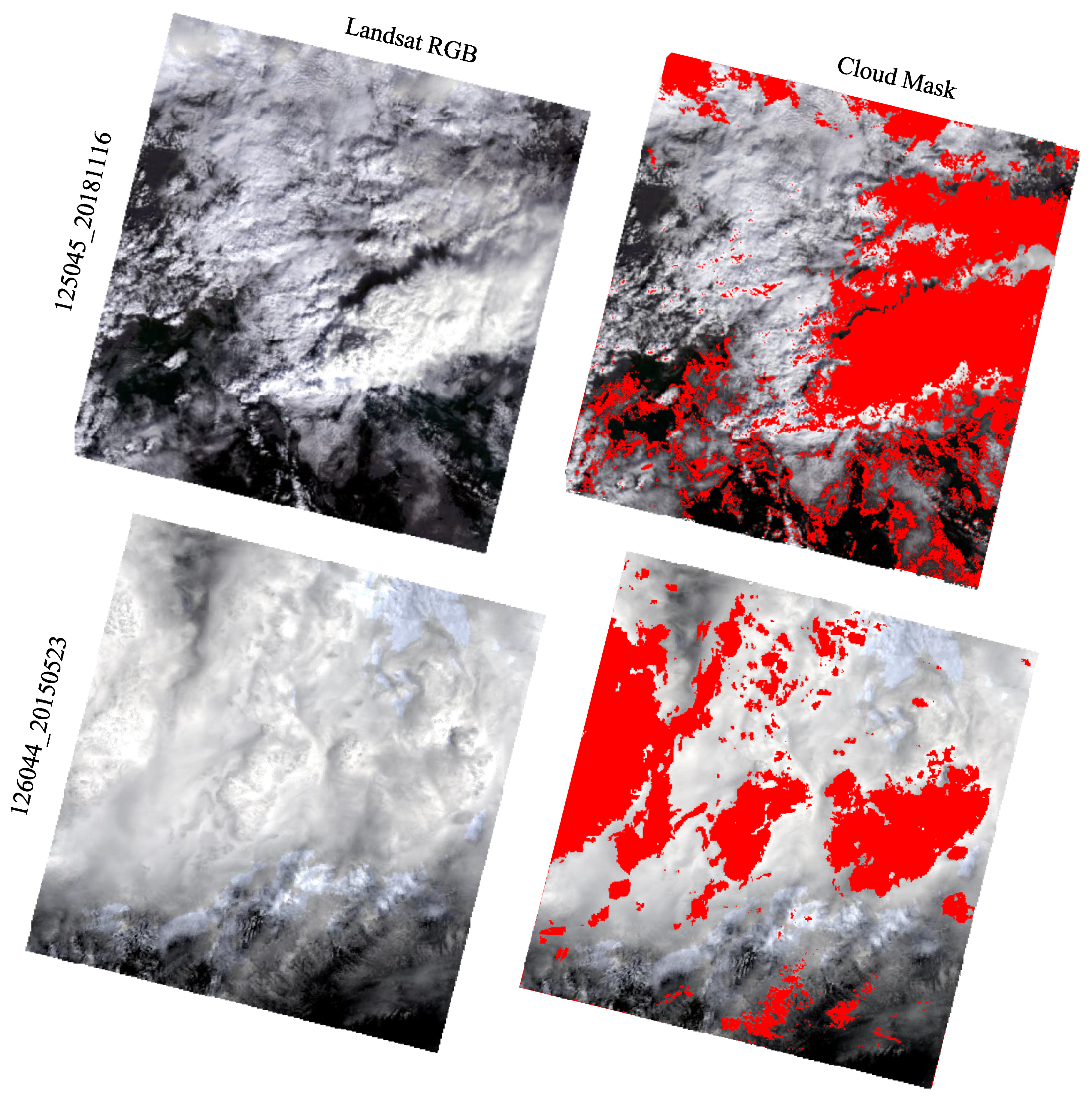
3.1. Pre-Processing
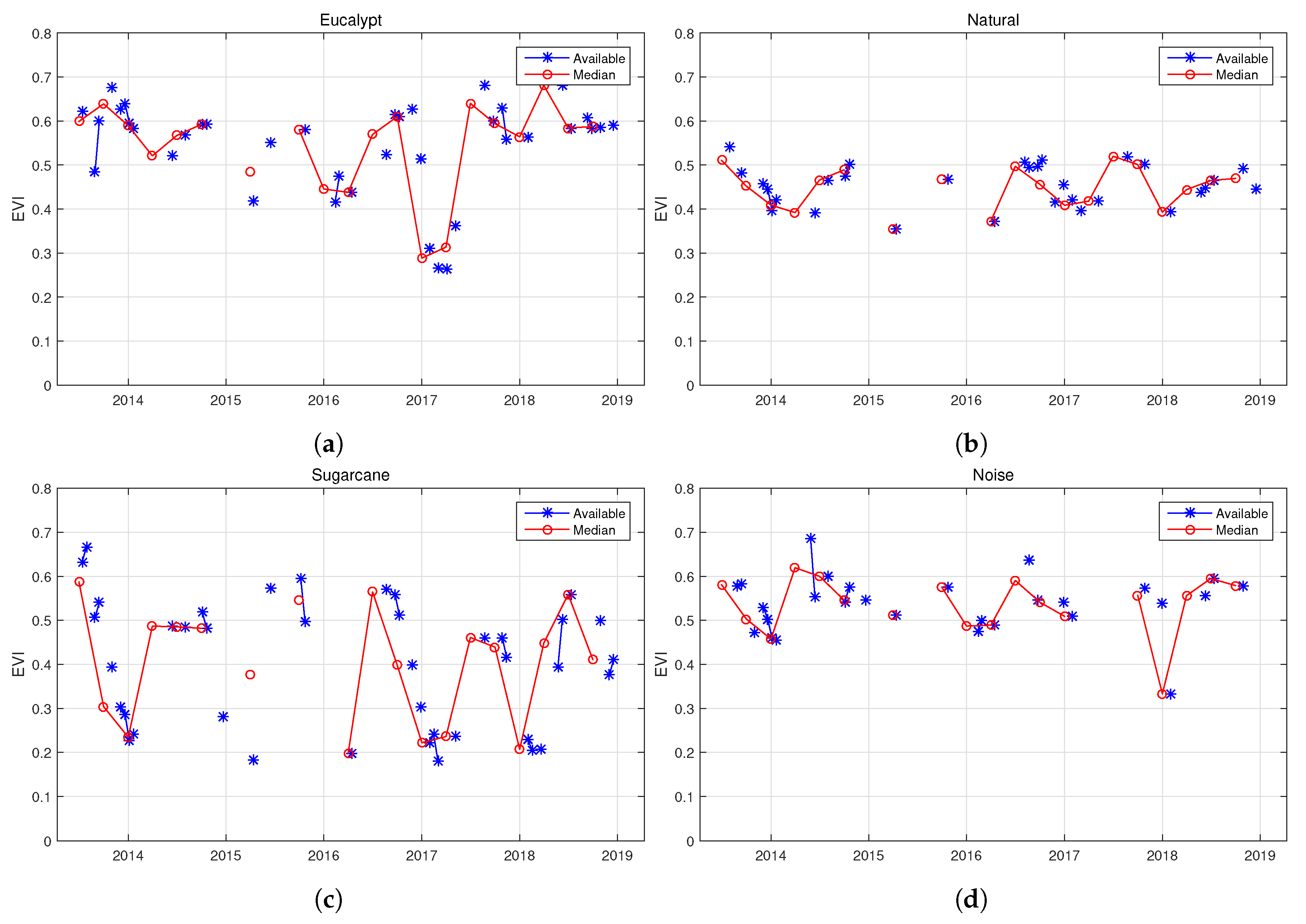
3.2. Clear-Cut Detection
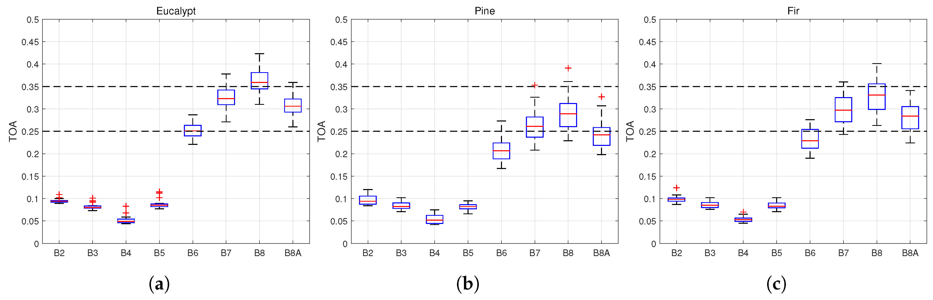
3.3. Broadleaf/Needleleaf Classification
3.4. Refinements Based on Superpixels
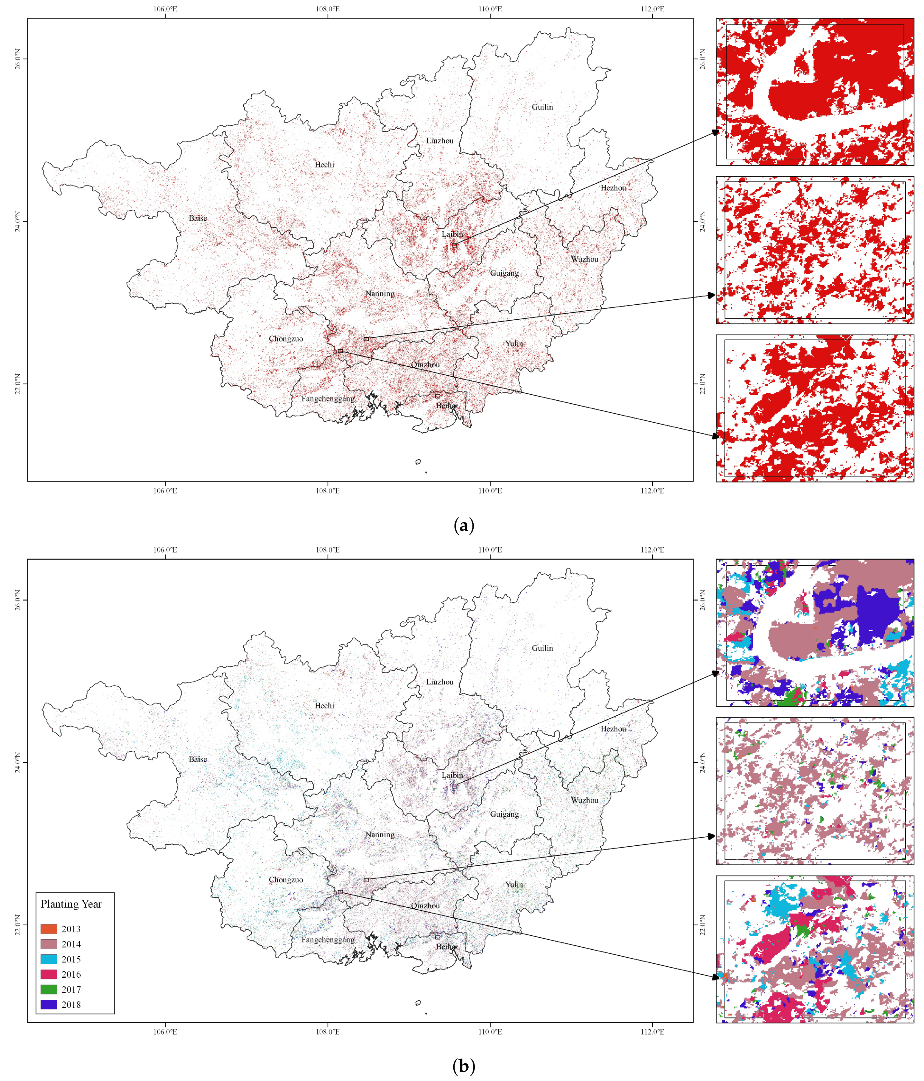
4. Result and Assessment
5. Discussions
6. Conclusions
Author Contributions
Funding
Acknowledgments
Conflicts of Interest
References
- Kennedy, R.E.; Cohen, W.B.; Schroeder, T.A. Trajectory-based change detection for automated characterization of forest disturbance dynamics. Remote Sens. Environ. 2007, 110, 370–386. [Google Scholar] [CrossRef]
- Kennedy, R.E.; Yang, Z.; Cohen, W.B. Detecting trends in forest disturbance and recovery using yearly Landsat time series: 1. LandTrendr - Temporal segmentation algorithms. Remote Sens. Environ. 2010, 114, 2897–2910. [Google Scholar] [CrossRef]
- Huang, C.; Goward, S.N.; Masek, J.G.; Thomas, N.; Zhu, Z.; Vogelmann, J.E. An automated approach for reconstructing recent forest disturbance history using dense Landsat time series stacks. Remote Sens. Environ. 2010, 114, 183–198. [Google Scholar] [CrossRef]
- Langner, A.; Miettinen, J.; Kukkonen, M.; Vancutsem, C.; Simonetti, D.; Vieilledent, G.; Verhegghen, A.; Gallego, J.; Stibig, H.J. Towards Operational Monitoring of Forest Canopy Disturbance in Evergreen Rain Forests: A Test Case in Continental Southeast Asia. Remote Sens. 2018, 10, 544. [Google Scholar] [CrossRef] [Green Version]
- Hansen, M.C.; Potapov, P.V.; Moore, R.; Hancher, M.; Turubanova, S.A.; Tyukavina, A.; Thau, D.; Stehman, S.V.; Goetz, S.J.; Loveland, T.R.; et al. High-Resolution Global Maps of 21st-Century Forest Cover Change. Science 2013, 342, 850–853. [Google Scholar] [CrossRef] [PubMed] [Green Version]
- Le Maire, G.; Dupuy, S.; Nouvellon, Y.; Loos, R.A.; Hakamada, R. Mapping short-rotation plantations at regional scale using MODIS time series: Case of eucalypt plantations in Brazil. Remote Sens. Environ. 2014, 152, 136–149. [Google Scholar] [CrossRef]
- MacDicken, K.; Jonsson, Ö.; Piña, L.; Maulo, S.; Contessa, V.; Adikari, Y.; Garzuglia, M.; Lindquist, E.; Reams, G.; D’Annunzio, R. Global Forest Resources Assessment 2015. How are the World’s Forests Changing? 2nd ed.; FAO: Rome, Italy, 2016. [Google Scholar]
- Zhang, C.; Fu, S. Allelopathic effects of eucalyptus and the establishment of mixed stands of eucalyptus and native species. For. Ecol. Manag. 2009, 258, 1391–1396. [Google Scholar] [CrossRef]
- Tan, Z.H.; Zhang, Y.P.; Song, Q.H.; Liu, W.J.; Deng, X.B.; Tang, J.W.; Deng, Y.; Zhou, W.J.; Yang, L.Y.; Yu, G.R.; et al. Rubber plantations act as water pumps in tropical China. Geophys. Res. Lett. 2011, 38. [Google Scholar] [CrossRef] [Green Version]
- Vihervaara, P.; Marjokorpi, A.; Kumpula, T.; Walls, M.; Kamppinen, M. Ecosystem services of fast-growing tree plantations: A case study on integrating social valuations with land-use changes in Uruguay. For. Policy Econ. 2012, 14, 58–68. [Google Scholar] [CrossRef]
- FAO. Global Planted Forests Thematic Study: Results and Analysis; Lungo, A.D., Ball, J., Carle, J., Eds.; Planted Forests and Trees Working Paper 38; FAO: Rome, Italy, 2006; Available online: www.fao.org/forestry/fra/38995/en (accessed on 4 July 2020).
- FAO. Eucalyptus in East Africa: Socio-Economic and Environmental Issues; Dessie, G., Erkossa, T., Eds.; Planted Forests and Trees Working Paper 46/E; FAO: Rome, Italy, 2011; unpublished. [Google Scholar]
- Jagger, P.; Pender, J. The role of trees for sustainable management of less-favored lands: The case of eucalyptus in Ethiopia. For. Policy Econ. 2003, 5, 83–95. [Google Scholar] [CrossRef] [Green Version]
- Zinn, Y.; Resck, D.V.; da Silva, J.E. Soil organic carbon as affected by afforestation with Eucalyptus and Pinus in the Cerrado region of Brazil. For. Ecol. Manag. 2002, 166, 285–294. [Google Scholar] [CrossRef]
- Forrester, D.I.; Bauhus, J.; Cowie, A.L.; Vanclay, J.K. Mixed-species plantations of Eucalyptus with nitrogen-fixing trees: A review. For. Ecol. Manag. 2006, 233, 211–230. [Google Scholar] [CrossRef] [Green Version]
- Qiao, H.; Wu, M.; Shakir, M.; Wang, L.; Kang, J.; Niu, Z. Classification of Small-Scale Eucalyptus Plantations Based on NDVI Time Series Obtained from Multiple High-Resolution Datasets. Remote Sens. 2016, 8, 117. [Google Scholar] [CrossRef] [Green Version]
- Chen, J.; Chen, J.; Liao, A.; Cao, X.; Chen, L.; Chen, X.; He, C.; Han, G.; Peng, S.; Lu, M.; et al. Global land cover mapping at 30 m resolution: A POK-based operational approach. ISPRS J. Photogramm. Remote Sens. 2015, 103, 7–27. [Google Scholar] [CrossRef] [Green Version]
- Esch, T.; Üreyen, S.; Zeidler, J.; Metz–Marconcini, A.; Hirner, A.; Asamer, H.; Tum, M.; Böttcher, M.; Kuchar, S.; Svaton, V.; et al. Exploiting big earth data from space - first experiences with the timescan processing chain. Big Earth Data 2018, 2, 36–55. [Google Scholar] [CrossRef] [Green Version]
- Gorelick, N.; Hancher, M.; Dixon, M.; Ilyushchenko, S.; Thau, D.; Moore, R. Google Earth Engine: Planetary-scale geospatial analysis for everyone. Remote Sens. Environ. 2017, 202, 18–27. [Google Scholar] [CrossRef]
- Esch, T.; Uereyen, S.; Asamer, H.; Hirner, A.; Marconcini, M.; Metz, A.; Zeidler, J.; Boettcher, M.; Permana, H.; Brito, F.; et al. Earth observation-supported service platform for the development and provision of thematic information on the built environment—The TEP-Urban project. In Proceedings of the 2017 Joint Urban Remote Sensing Event (JURSE), Dubai, UAE, 6–8 March 2017; pp. 1–4. [Google Scholar] [CrossRef]
- Dong, J.; Xiao, X.; Menarguez, M.A.; Zhang, G.; Qin, Y.; Thau, D.; Biradar, C.; Moore, B. Mapping paddy rice planting area in northeastern Asia with Landsat 8 images, phenology-based algorithm and Google Earth Engine. Remote Sens. Environ. 2016, 185, 142–154. [Google Scholar] [CrossRef] [Green Version]
- Xiong, J.; Thenkabail, P.S.; Gumma, M.K.; Teluguntla, P.; Poehnelt, J.; Congalton, R.G.; Yadav, K.; Thau, D. Automated cropland mapping of continental Africa using Google Earth Engine cloud computing. ISPRS J. Photogramm. Remote Sens. 2017, 126, 225–244. [Google Scholar] [CrossRef] [Green Version]
- Teluguntla, P.; Thenkabail, P.S.; Oliphant, A.; Xiong, J.; Gumma, M.K.; Congalton, R.G.; Yadav, K.; Huete, A. A 30-m landsat-derived cropland extent product of Australia and China using random forest machine learning algorithm on Google Earth Engine cloud computing platform. ISPRS J. Photogramm. Remote Sens. 2018, 144, 325–340. [Google Scholar] [CrossRef]
- Koskinen, J.; Leinonen, U.; Vollrath, A.; Ortmann, A.; Lindquist, E.; d’Annunzio, R.; Pekkarinen, A.; Käyhkö, N. Participatory mapping of forest plantations with Open Foris and Google Earth Engine. ISPRS J. Photogramm. Remote Sens. 2019, 148, 63–74. [Google Scholar] [CrossRef]
- Forestry Bureau of Guangxi. The Planning and Development of Guangxi Forestry Industry in The 13th Five-Year. 2018. Available online: http://www.gxly.cn/Upload/file/20180521/20180521175756_8592.doc (accessed on 18 June 2019). (In Chinese).
- Liu, J.Y.; Zhuang, D.F.; Luo, D.; Xiao, X. Land-cover classification of China: Integrated analysis of AVHRR imagery and geophysical data. Int. J. Remote. Sens. 2003, 24, 2485–2500. [Google Scholar] [CrossRef]
- Chen, J.; Ban, Y.; Li, S. China: Open access to Earth land-cover map. Nature 2014, 514, 434. [Google Scholar]
- Hu, Y.; Zhen, L.; Zhuang, D. Assessment of Land-Use and Land-Cover Change in Guangxi, China. Sci. Rep. 2019, 9, 2189. [Google Scholar] [CrossRef] [PubMed] [Green Version]
- Huete, A.; Didan, K.; Miura, T.; Rodriguez, E.; Gao, X.; Ferreira, L. Overview of the radiometric and biophysical performance of the MODIS vegetation indices. Remote Sens. Environ. 2002, 83, 195–213. [Google Scholar] [CrossRef]
- Zhu, Z.; Wang, S.; Woodcock, C.E. Improvement and expansion of the Fmask algorithm: Cloud, cloud shadow, and snow detection for Landsats 4-7, 8, and Sentinel 2 images. Remote Sens. Environ. 2015, 159, 269–277. [Google Scholar] [CrossRef]
- Vermote, E.; Justice, C.; Claverie, M.; Franch, B. Preliminary analysis of the performance of the Landsat 8/OLI land surface reflectance product. Remote Sens. Environ. 2016, 185, 46–56. [Google Scholar] [CrossRef]
- Maiersperger, T.; Scaramuzza, P.; Leigh, L.; Shrestha, S.; Gallo, K.; Jenkerson, C.; Dwyer, J. Characterizing LEDAPS surface reflectance products by comparisons with AERONET, field spectrometer, and MODIS data. Remote Sens. Environ. 2013, 136, 1–13. [Google Scholar] [CrossRef] [Green Version]
- Feng, M.; Sexton, J.O.; Huang, C.; Masek, J.G.; Vermote, E.F.; Gao, F.; Narasimhan, R.; Channan, S.; Wolfe, R.E.; Townshend, J.R. Global surface reflectance products from Landsat: Assessment using coincident MODIS observations. Remote Sens. Environ. 2013, 134, 276–293. [Google Scholar] [CrossRef]
- Ye, S.; Rogan, J.; Sangermano, F. Monitoring rubber plantation expansion using Landsat data time series and a Shapelet-based approach. ISPRS J. Photogramm. Remote Sens. 2018, 136, 134–143. [Google Scholar] [CrossRef]
- Fernández-Manso, A.; Fernández-Manso, O.; Quintano, C. SENTINEL-2A red-edge spectral indices suitability for discriminating burn severity. Int. J. Appl. Earth Obs. Geoinf. 2016, 50, 170–175. [Google Scholar] [CrossRef]
- Immitzer, M.; Vuolo, F.; Atzberger, C. First Experience with Sentinel-2 Data for Crop and Tree Species Classifications in Central Europe. Remote Sens. 2016, 8, 166. [Google Scholar] [CrossRef]
- Forkuor, G.; Dimobe, K.; Serme, I.; Tondoh, J. Landsat-8 vs. Sentinel-2: Examining the added value of Sentinel-2’s red-edge bands to land-use and land-cover mapping in Burkina Faso. Gisci. Remote Sens. 2017. [Google Scholar] [CrossRef]
- Wessel, M.; Brandmeier, M.; Tiede, D. Evaluation of Different Machine Learning Algorithms for Scalable Classification of Tree Types and Tree Species Based on Sentinel-2 Data. Remote Sens. 2018, 10, 1419. [Google Scholar] [CrossRef] [Green Version]
- Sothe, C.; Almeida, C.M.D.; Liesenberg, V.; Schimalski, M.B. Evaluating Sentinel-2 and Landsat-8 Data to Map Sucessional Forest Stages in a Subtropical Forest in Southern Brazil. Remote Sens. 2017, 9, 838. [Google Scholar] [CrossRef] [Green Version]
- Huang, C.; Davis, L.S.; Townshend, J.R.G. An assessment of support vector machines for land cover classification. Int. J. Remote Sens. 2002, 23, 725–749. [Google Scholar] [CrossRef]
- Mountrakis, G.; Im, J.; Ogole, C. Support vector machines in remote sensing: A review. ISPRS J. Photogramm. Remote Sens. 2011, 66, 247–259. [Google Scholar] [CrossRef]
- Blaschke, T. Object based image analysis for remote sensing. ISPRS J. Photogramm. Remote Sens. 2010, 65, 2–16. [Google Scholar] [CrossRef] [Green Version]
- Myint, S.W.; Gober, P.; Brazel, A.; Grossman-Clarke, S.; Weng, Q. Per-pixel vs. object-based classification of urban land cover extraction using high spatial resolution imagery. Remote Sens. Environ. 2011, 115, 1145–1161. [Google Scholar] [CrossRef]
- Hussain, M.; Chen, D.; Cheng, A.; Wei, H.; Stanley, D. Change detection from remotely sensed images: From pixel-based to object-based approaches. ISPRS J. Photogramm. Remote Sens. 2013, 80, 91–106. [Google Scholar] [CrossRef]
- Achanta, R.; Susstrunk, S. Superpixels and Polygons using Simple Non-Iterative Clustering. In Proceedings of the IEEE Conference on Computer Vision and Pattern Recognition (CVPR), Honolulu, HI, USA, 21–26 July 2017. [Google Scholar]


| District | Area (ha) | % of Land Area |
|---|---|---|
| Baise | 123,659.73 | 3.10% |
| Beihai | 44,619.39 | 11.88% |
| Chongzuo | 98,650.98 | 5.22% |
| Fangchenggang | 57,632.76 | 8.86% |
| Guigang | 78,898.50 | 6.79% |
| Guilin | 35,009.64 | 1.14% |
| Hechi | 124,611.66 | 3.38% |
| Hezhou | 45,170.10 | 3.51% |
| Laibin | 163,282.95 | 11.30% |
| Liuzhou | 100,117.26 | 4.80% |
| Nanning | 210,990.60 | 8.74% |
| Qinzhou | 150,095.16 | 12.91% |
| Wuzhou | 87,910.92 | 6.45% |
| Yulin | 118,571.85 | 8.48% |
| Total | 1,439,221.50 | 5.54% |
| Samples | Eucalypt (Detected) | Non-Eucalypt (Detected) | Producer’s Accuracy |
| Eucalypt (Reference) | 1374 | 778 | 63.85% |
| Non-Eucalypt (Reference) | 680 | 9285 | 93.18% |
| User’s Accuracy | 66.89% | 92.27% | 87.97% |
| ROI | Eucalypt (Detected) | Non-Eucalypt (Detected) | Producer’s Accuracy |
| Eucalypt (Reference) | 22,547 | 14,946 | 60.14% |
| Non-Eucalypt (Reference) | 11,876 | 369,177 | 96.88% |
| User’s Accuracy | 65.50% | 96.11% | 93.59% |
| SVM | Eucalypt (Detected) | Non-Eucalypt (Detected) | Producer’s Accuracy |
| Eucalypt (Reference) | 971 | 1181 | 45.12% |
| Non-Eucalypt (Reference) | 2489 | 7476 | 75.02% |
| User’s Accuracy | 28.06% | 86.36% | 69.71% |
| Year | Area (ha) |
|---|---|
| 2013 | 155,538.91 |
| 2014 | 565,096.22 |
| 2015 | 239,765.04 |
| 2016 | 129,719.43 |
| 2017 | 154,069.11 |
| 2018 | 195,032.79 |
© 2020 by the authors. Licensee MDPI, Basel, Switzerland. This article is an open access article distributed under the terms and conditions of the Creative Commons Attribution (CC BY) license (http://creativecommons.org/licenses/by/4.0/).
Share and Cite
Deng, X.; Guo, S.; Sun, L.; Chen, J. Identification of Short-Rotation Eucalyptus Plantation at Large Scale Using Multi-Satellite Imageries and Cloud Computing Platform. Remote Sens. 2020, 12, 2153. https://0-doi-org.brum.beds.ac.uk/10.3390/rs12132153
Deng X, Guo S, Sun L, Chen J. Identification of Short-Rotation Eucalyptus Plantation at Large Scale Using Multi-Satellite Imageries and Cloud Computing Platform. Remote Sensing. 2020; 12(13):2153. https://0-doi-org.brum.beds.ac.uk/10.3390/rs12132153
Chicago/Turabian StyleDeng, Xinping, Shanxin Guo, Luyi Sun, and Jinsong Chen. 2020. "Identification of Short-Rotation Eucalyptus Plantation at Large Scale Using Multi-Satellite Imageries and Cloud Computing Platform" Remote Sensing 12, no. 13: 2153. https://0-doi-org.brum.beds.ac.uk/10.3390/rs12132153