Next Article in Journal
Understanding the Land Surface Phenology and Gross Primary Production of Sugarcane Plantations by Eddy Flux Measurements, MODIS Images, and Data-Driven Models
Next Article in Special Issue
Correction: Niculescu, S., et al. Synergy of High-Resolution Radar and Optical Images Satellite for Identification and Mapping of Wetland Macrophytes on the Danube Delta. Remote Sensing 2020, 12(14), 2188
Previous Article in Journal
Soil Conservation Service Spatiotemporal Variability and Its Driving Mechanism on the Guizhou Plateau, China
 
 
Correction published on 6 August 2020, see Remote Sens. 2020, 12(16), 2529.
Article

Synergy of High-Resolution Radar and Optical Images Satellite for Identification and Mapping of Wetland Macrophytes on the Danube Delta

1
Department of Geography, University of Western Brittany, 3 Rue des Archives, 29238 Brest, France
2
Department of Geography, University of Rennes 2, Place Recteur Henri le Moal, 35000 Rennes, France
3
ONF International, 45 bis avenue de la Belle Gabrielle, 94736 Nogent-sur-Marne, France
4
Department of Geography, University Santa Barbara, Santa Barbara, CA 93106, USA
5
Danube Delta National Institute for Research and Development, Strada Babadag nr. 165, Tulcea 820112, Romania
*
Author to whom correspondence should be addressed.
Remote Sens. 2020, 12(14), 2188; https://0-doi-org.brum.beds.ac.uk/10.3390/rs12142188
Submission received: 22 May 2020 / Revised: 3 July 2020 / Accepted: 5 July 2020 / Published: 8 July 2020
(This article belongs to the Special Issue Remote Sensing of Wetland Vegetation Patterns and Dynamics)

Abstract

:
In wetland environments, vegetation has an important role in ecological functioning. The main goal of this work was to identify an optimal combination of Sentinel-1 (S1), Sentinel-2 (S2), and Pleiades data using ground-reference data to accurately map wetland macrophytes in the Danube Delta. We tested several combinations of optical and Synthetic Aperture Radar (SAR) data rigorously at two levels. First, in order to reduce the confusion between reed (Phragmites australis (Cav.) Trin. ex Steud.) and other macrophyte communities, a time series analysis of S1 data was performed. The potential of S1 for detection of compact reed on plaur, compact reed on plaur/reed cut, open reed on plaur, pure reed, and reed on salinized soil was evaluated through time series of backscatter coefficient and coherence ratio images, calculated mainly according to the phenology of the reed. The analysis of backscattering coefficients allowed separation of reed classes that strongly overlapped. The coherence coefficient showed that C-band SAR repeat pass interferometric coherence for cut reed detection is feasible. In the second section, random forest (RF) classification was applied to the S2, Pleiades, and S1 data and in situ observations to discriminate and map reed against other aquatic macrophytes (submerged aquatic vegetation (SAV), emergent macrophytes, some floating broad-leaved and floating vegetation of delta lakes). In addition, different optical indices were included in the RF. A total of 67 classification models were made in several sensor combinations with two series of validation samples (with the reed and without reed) using both a simple and more detailed classification schema. The results showed that reed is completely discriminable compared to other macrophyte communities with all sensor combinations. In all combinations, the model-based producer’s accuracy (PA) and user’s accuracy (UA) for reed with both nomenclatures were over 90%. The diverse combinations of sensors were valuable for improving the overall classification accuracy of all of the communities of aquatic macrophytes except Myriophyllum spicatum L.

Graphical Abstract

1. Introduction

Wetlands are described as “the lands of transition zone between aquatic and terrestrial ecosystems where the land is covered by shallow water” [1]. Wetlands (marshes, peat bogs, coastal mudflats, alluvial forests, etc.) form a complex set of environments. They have a high biological productivity and great biological diversity and are considered dynamic ecologically. Wetland vegetation is an important component of wetland ecosystems and plays an important role in maintaining ecosystem structure and function [2]. Wetland vegetation ecosystems depend on water levels and therefore climate change, especially changes in precipitation, is likely to have a significant impact on these habitats and associated species. Phragmites australis (common reed) is one of the most widely distributed wetland macrophyte plant species. Reed is a key species and plays a significant role in wetland ecosystems, with high biomass and abundance.
Aquatic macrophytes are also key components of wetland ecosystems. Knowing the function of aquatic macrophytes in wetlands and shallow lake ecosystems is critical for understanding basic ecosystem processes. It is also important for numerous applications, such as wetland restoration, wastewater treatment, and management of invasive species [3]. Accurate wetland vegetation mapping is needed to distinguish the different classes of macrophyte vegetation, understand their functions, and analyze the response of wetlands to climate change and human activities. Recently, remote sensing methodology for the study of wetland vegetation has been used by many researchers [4,5,6,7,8,9,10,11].
Advances in sensors and data analysis techniques have made remote sensing a means of monitoring vegetation in wetlands. Optical remote sensing data have been used widely since the 1970s to study vegetation and the environment [12]. In order to improve the accuracy of research, several scholars have recently used fine spatial resolution images in vegetation wetland studies [13,14,15,16,17]. Fine spatial resolution images offer many advantages for the identification of wetland boundaries and plant formations. In this study, the optical domain was used to differentiate submergent macrophytes from emergent vegetation. Aquatic plants and their properties, however, are not as easily detected as terrestrial vegetation. The major difficulty for the classification of aquatic macrophytes is the modification of the reflectance by the water column. The water column absorbs part of the radiation from aquatic plants and makes them more difficult to detect. Elements in the water column, such as plankton or sediment, also modify the optical signal and further complicate species detection. Some research also recommends including bathymetric information in models and classifications to reduce the influence of the water column [18]. At the leaf level, the presence and concentration of leaf pigments determines the response in the visible region of the spectrum, and leaf morphology and water content are the main factors acting in the near-infrared. At the individual level, biophysical factors such as leaf distribution, leaf density and orientation, and overall canopy structure are important [18]. In the same study, Silva et al., [18] highlight the difference between detection of submergent and emergent macrophytes. Submergent macrophytes are much more difficult to detect because the plants are not visible on the surface. Aquatic plant reflectance can also vary greatly depending on the phenological stage of the plant, which is important in choosing the date of the image to be processed. This variability also explains the recurring confusion between emergent macrophytes and terrestrial vegetation. Another important factor is the density of a macrophyte surface, which as it increases will also increase canopy reflectance in the Near-infrared (NIR) wavelengths (between 700 and 1000 nanometers).
Radar may be relevant for studying aquatic macrophytes because of the ability of microwaves to distinguish dry vegetation from moist or even submerged vegetation. The longer microwave wavelengths penetrate into the canopy, resulting in a “volumetric” signal. However, as radar wavelengths do not penetrate into water, radar systems can only be applied to emergent macrophytes. For backscatter, the radar response to aquatic vegetation is similar to that of terrestrial species, with predominantly volume and geometric scattering.
It is difficult to monitor vegetation within wetlands only using optical images because the dense vegetation cover leads to signal saturation [19] and because of very high spatial and spectral variability, due to very short ecotones between wetland vegetation units [20,21,22]. In this context, radar imagery is widely used in mapping wetlands. Radar data provide completely different information from sensors that operate in the visible and near-infrared range of the electromagnetic spectrum. For some years now, a new generation of radar images has been available. Radar systems have great potential for delineating wetland characteristics, including species composition, water surface detection, vegetation health, or structural properties [23,24,25]. Many studies have demonstrated the importance of microwave sensors for vegetation monitoring [26,27,28,29].
In this study, Sentinel-1 (S1) radar (C band) was used to distinguish macrophyte vegetation such as several classes of reed (Phragmites australis) compared to other macrophyte communities. Two reed surfaces were observed: compact reed (dense reed) and cut reed. The period of cut in the Danube Delta is from November to March. Most scholars agree that the radar signal is the sum of several components: diffuse scattering of the soil surface, volume scattering by vegetation, and multiple interactions between vegetation and soil. In our case, the soil contributes very little to the signal because most surfaces are made up of water (according to the phenological calendar of the reed (Figure 1a). The growth of the reed results in an increase in the height of the stems and the number and the size of the leaves. The contribution of each component to the total radar signal depends on the characteristics of the reed, the soil (roughness and moisture content)/water, and other parameters (incidence and polarization). For dense reed surfaces, the radar signal is composed of the double-bounce interaction from the radiation and return to the sensor (Figure 1b), the surface backscatter from the ground surface and the volumetric backscatter from the canopy elements, the result of the interaction of the radiation within the vegetation canopy, leaves, and stems (Figure 1c). For cut reed, the surfaces are composed of water and less dense leftover stems. For similar surfaces (herbaceous plants in flooded wetlands), Pope et al. [30] observed that the backscattering values are not as high as those observed for high density stands due to the increase in the forward scattering in water patches.
The information potential of radar images with regard to the inventory and mapping of vegetation is highlighted by analyzing these images in combination with optical images. Recently, processes such as stacking, coregistration, and data fusion of optical with radar products have been applied to improve classification quality and its accuracy. Multi-source integration should be the trend of future wetland remote sensing [12]. A combination of data from multiple sensors can achieve a high level of accuracy in the classification of vegetation in the Danube Delta [31,32]. A data fusion approach combining SAR data, optical multi-spectral data, and airborne laser scanning light detection and ranging (LIDAR) for wetland vegetation detection was conducted by Niculescu et al. [31] in the Danube Delta. In recent years, machine learning approaches such as support vector machine (SVM), random forests (RF), and artificial neural networks (ANN) have become very popular classifiers for SAR data or optical data classification, as they can provide accurate wetland maps [32,33,34,35]. RF, used in this study, has also been successful in many studies of classification of vegetation and complex environments, such as wetlands [36,37,38].
The main goal of this research was to distinguish and map Phragmites australis from aquatic machrophytes (submerged aquatic vegetation (SAV), emergent macrophytes, and some floating broad-leaved) in the Danube Delta using time series of the S1 (high spatial resolution radar images) and Sentinel-2 (S2) (high spatial resolution optical images) and Pleiades images (very high spatial resolution optical images). The novelty of this study resides in determination of the optimal combination of sensors, periods of observations, diverse nomenclatures, different environments of wetlands and an adapted methodology for reducing confusion in discriminating several classes of the Phragmites australis (compact reed on plaur, compact reed on plaur/reed cut, open reed on plaur, pure reed, and reed on salinized soil) and aquatic macrophytes within the lakes of delta. The S1 time-series radar was used to distinguish the different types of surface covers by the many classes of reed, including cut reed. In this first section, the potential of S1 is evaluated through time series of the backscatter coefficient and coherence ratio images, calculated mainly according to the phenology of the reed. In the second section, RF was used to build up classification models in three different sensor combinations: the first using only S1 data, the second using only S2 data, and the third using both S1 and S2 data. The RF classification model was used to test all data sets and select the most thematically accurate product for macrophyte wetlands in Danube Delta.

2. Materials and Methods

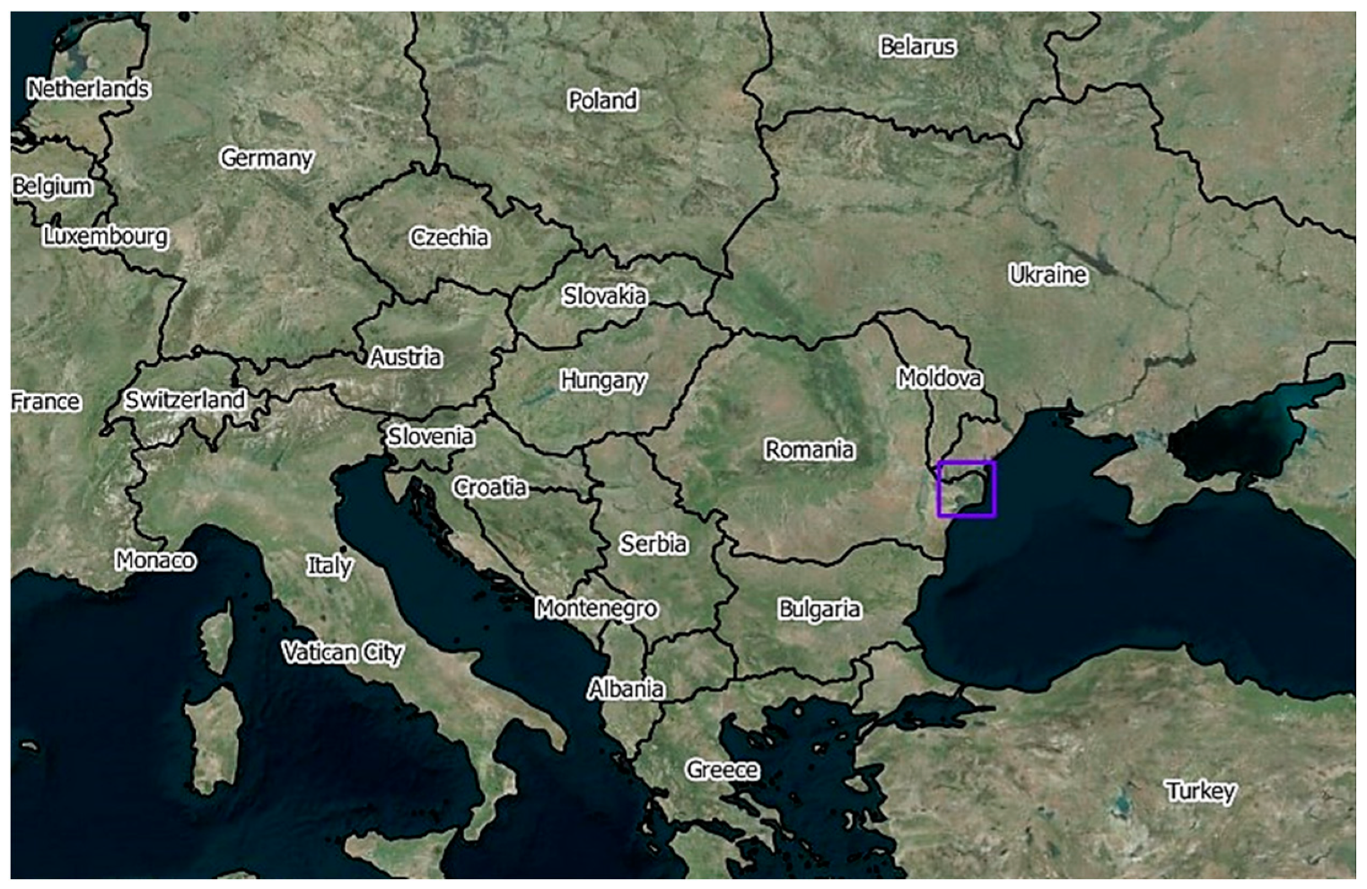
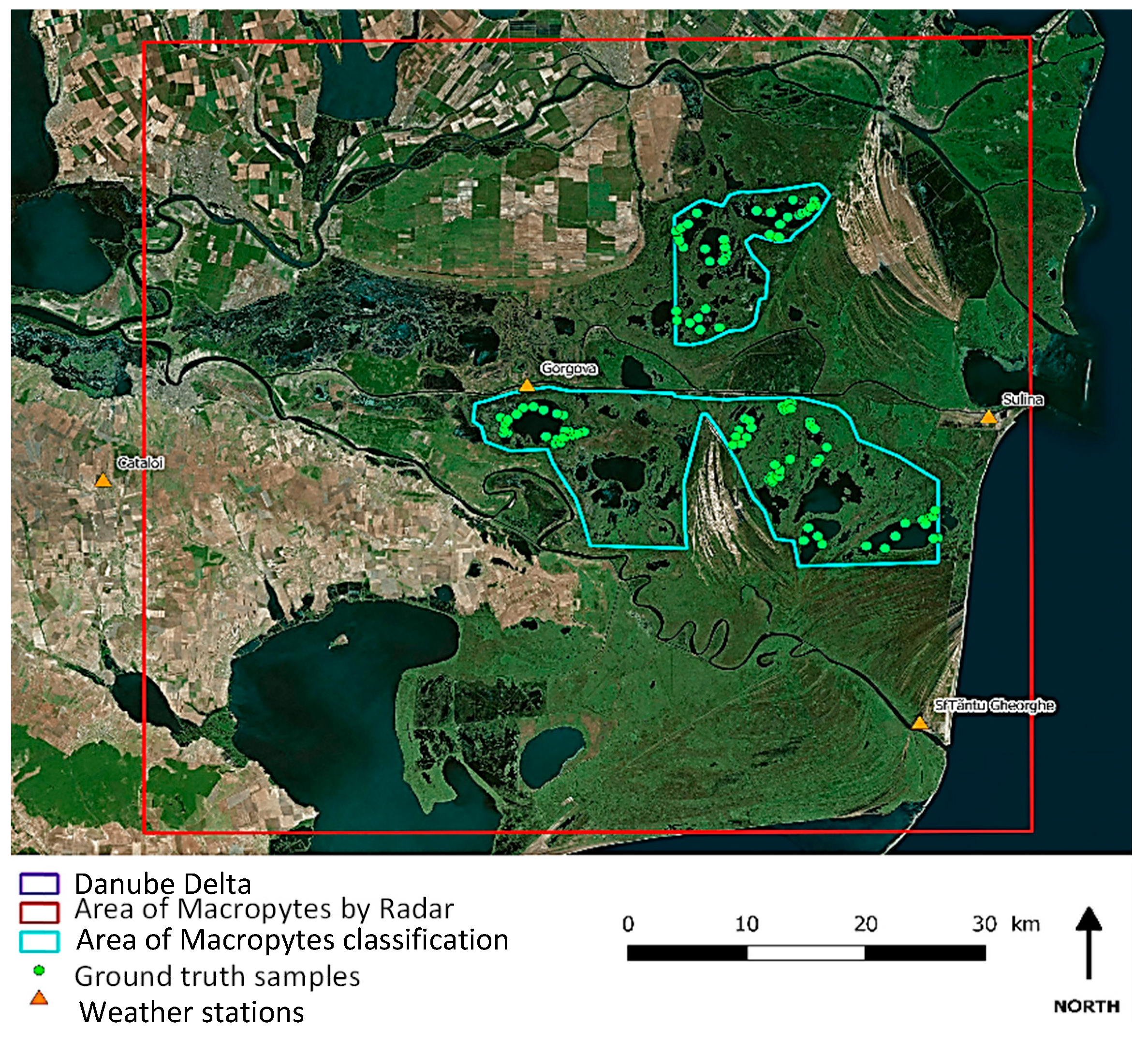
2.1. Study Area and Vegetation of Danube Delta

2.1.1. Study Area

The study was conducted in the Danube Delta (45°10′29″N, 29°22′58″E) (Figure 2). It is located in southeastern Romania and southern Ukraine. The delta consists mainly of wetland vegetation with lakes in the center and southwest, some forests and dune areas, some cities along the three main arms, and finally an agricultural area to the northwest.
Natural marsh vegetation dominated by reed (44%) and other aquatic vegetation (27%) is the most widespread class in the Danube Delta. The area covered by these vegetation classes is 398,676 ha, of which 362,965 ha is in the Romanian part and 35,711 ha is in the Ukrainian part [39].
For the section on the potential of radar to detect the many classes of Phragmites australis, the study area includes almost all the delta (red footprint, Figure 2). For the macrophyte classification section, two more boundaries were selected for lake areas (cyan, Figure 2). The two zones were chosen according of the overlap between the Pléiades satellite data, S1 and S2, and the terrain data.

2.1.2. Phragmites australis

Reed marshes, covering more than 220,000 hectares [39], are the Danube Delta’s most dominant vegetation unit. The first detailed vegetation map of the Danube Delta was based on aerial photo interpretation, satellite images, and verification through field checks [39]. Most of the photointerpretation was carried out at a scale 1:22,000 up to 1:25,000. The primary plant community is Scirpo-Phragmitetum Koch. The dominant species is Phragmites australis, usually accompanied by hydrophilous species as Typha angustifolia L., Carex sp., Schoenoplectus lacustris (L.) Palla and Thelypteris palustris (A. Gray) Schot. There is high variability in the floristic structure and composition of reed vegetation of the Danube Delta due to variation in the main ecological factors such as hydrology, soil substrate, and salinity. Such variation, in connection with biometrical parameters of the specific reed populations, determines the individual categorization of reed subassociations and distribution [39]. Bolboschoenus-Phragmitetum Borhidi and Balogh, creates a variable width band around the exterior edge of the marsh. Located on the edge of temporary flooded marshes, it grows on gleyic soil and moderate-to-strong saline arenosoils with low alkaline pH. It is recognized as a type of halophyle species. Astero tripolii-Phragmitetum Krisch is found on the shores of maritime areas that experience temporary, low levels of flooding and is prone to saline psammosoil and alkaline reactions. Another vegetation formation specific of the delta is floating reed beds covering around 109,000 ha [39]. Often, reed marshes are invaded by grey willow (Salix cinerea L.) bushes.
In this study, many classes of Phragmites australis were observed: compact reed on plaur, /reed cut, open reed on plaur, pure reed, and reed on salinized soil. In the Danube Delta, a local name for a peat marsh is “plaur”. In its initial stage, this reed peat is not connected either to the mineral lagoon bottom or to the lake bottom itself. It is literally a floating layer, consisting of a network of viable rhizomes (fibric peat) with a thickness of 0.8–1.3 m, often with many patches of water in it. The layer grows gradually thicker. Eventually it establishes contact with the mineral floor. In the final stage, the layer with viable rhizomes rests on layers of older and more mineralized peat (hemic or sapric peat).

2.1.3. Aquatic Macrophyte Vegetation

Over 300 lakes are found in the Danube Delta, and lake size varies from 14 to 4530 ha [40]. Lakes are supplied with fresh river water through vast networks of natural and artificial canals. The water level in lakes is variable and dependent on the river pulse. The highest water level is recorded in spring (May–June) [40]. With water depths of 1.5–4 m and a chloride concentration below 60 mg/L, the Danube Delta lakes are characterized as shallow freshwater lakes. Based on the classification scheme of Vollenweider [41], these lakes are eutrophic with respect to phosphorus.
There are strong differences in vegetation dominance between these lakes. These are the main controlling factors that play an important role in the distribution of aquatic macrophytes that influence the trophic gradient recognizing that most of the floodplain lakes are to some extent connected with a river [40,42,43]. In our data, we distinguished three type of lakes: (1) lakes with the highest connectivity dominated by Potamogeton trichoides Cham. & Schltdl., P. crispus, Elodea nuttallii, (2) long distance, large turbid lakes located at the deeper parts of the former marine lagoons with Potamogeton crispus L. and Myriophyllum spicatum, and (3) long distance lakes with low connectivity characterised by Nitellopsis obtusa (Desvaux in Loiseleur) J. Groves, Chara globularis Thuiller, Chara aspera Willdenow, Myriophyllum spicatum L., Myriophyllum verticillatum L., Stratiotes aloides L., Utricularia vulgaris L., Nuphar lutea (L.) Sm., Nymphaea alba L., Nymphaea candida C.Presl, Hydrocharis morsus-ranae L., and Nymphoides peltata (S.G.Gmel.) Kuntze.

2.2. Data Set

2.2.1. Satellite Data

Three types of satellite data were used. For the radar domain, S1 data using both systems (1A and 1B) were used. The Copernicus Sentinel-1 mission, operated by the European Space Agency, provides the opportunity to monitor Earth’s surface using radar at high spatial and temporal resolution. The Sentinel-1 satellites carry synthetic aperture radars (SAR), providing backscatter at C-band (5.405 GHz). They have a spatial resolution of 10 m and a temporal resolution of 12 days (6 by combining the two satellites) and can take images according to several modes of acquisition. The “interferometric wide swath” (IW) mode was used in this study. It facilitates interferometry and provides images with a swath width of 250 km. Fifty-nine images were downloaded on the Plateforme d’exploitation des produits Sentinel (PEPS) platform (https://peps.cnes.fr) over the period 2016–2017, in “single look complex” (SLC) format and in “ground range detected” (GRD) format. The first includes the phase and intensity information of the radar signal, while the second contains only the intensity information.
For the optical domain, S2 and Pleiades data (Tables S1 and S2/Supplementary material) were used. The first is a pair of European satellites (2A and 2B). Their spatial resolution is 10, 20, or 60 m depending on the bands, providing a 5-day temporal resolution by combining the two satellites, and a 290 km swath. The Danube Delta is included on two footprints, and 76 images (38 for each path) were downloaded with processing level 1C (without atmospheric correction), also on the PEPS platform.
Pleiades data were provided by GEOSUD. Pleiades is a pair of French satellites (1A and 1B). They have four (4) bands (visible and NIR) acquired at 0.7 m spatial resolution and a panchromatic band at 0.5 m (Table S1/Supplementary material). The images acquired by the satellites have a swath of up to 100 km. The three images ordered were previously orthorectified, and the bands of the visible and PIR were resampled to 0.5 m spatial resolution from the panchromatic band by the supplier.
A summary of the properties of the three sensor types is included in Table 1.

2.2.2. Environmental Data
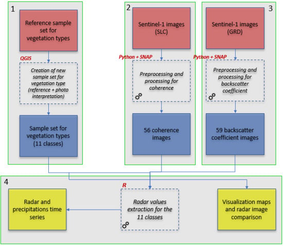
In order to compare the values of the radar images with the precipitation, daily data from four weather stations (Sfanta Gheorghe, Sulina, Gorgova, and Cataloi) (Figure 2) located on the delta acquired from 2016 to 2017 were downloaded from the NOAA platform: https://www7.ncdc.noaa.gov.

2.3. Methodology

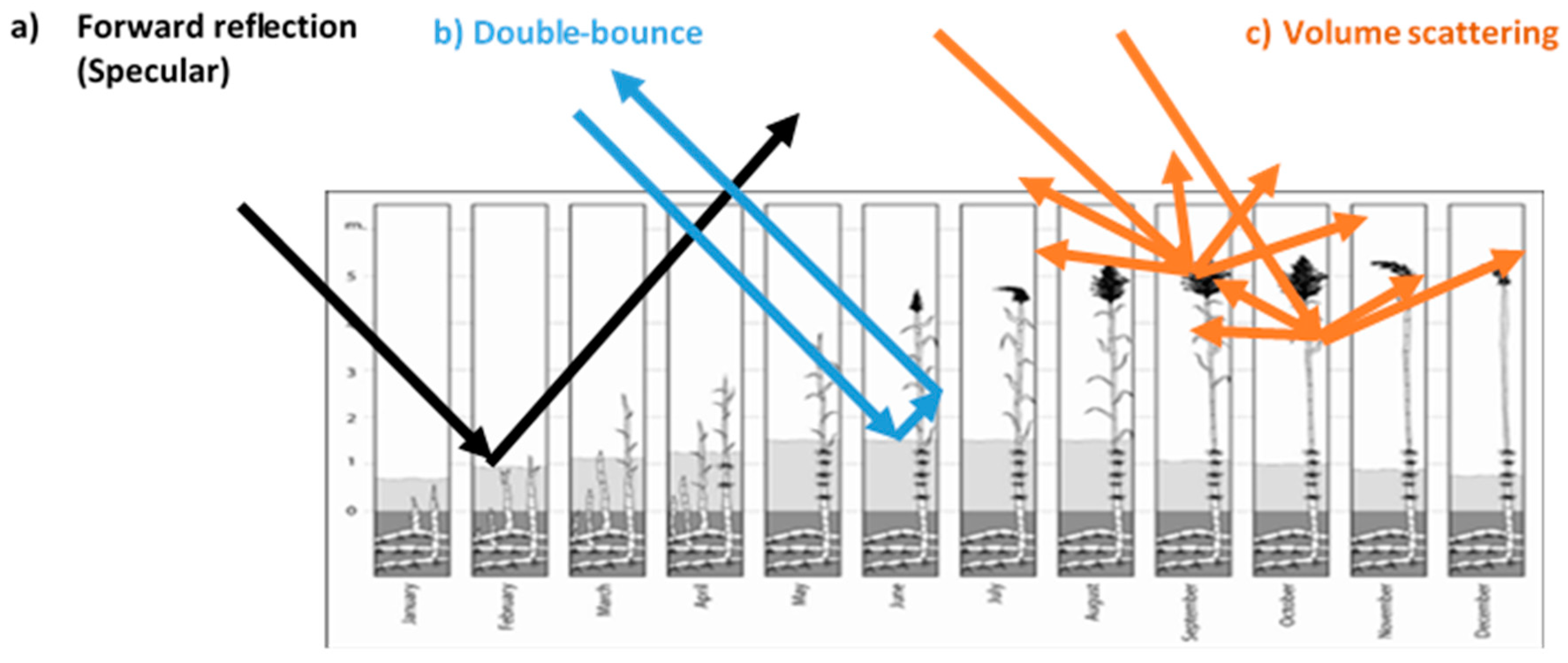
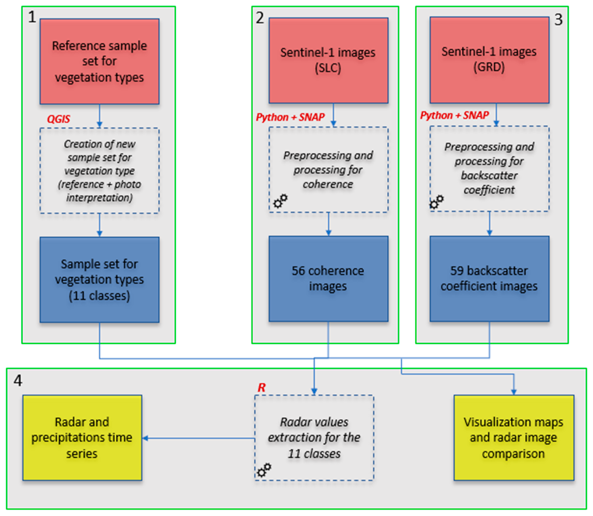
2.3.1. Backscatter Coefficient and Coherence Estimation

In the first section, several steps were applied: calculation of coherence from SLC Sentinel-1 data and calculation of backscatter coefficients from Sentinel-1 GRD data and extraction of the radar values from the sample set. In this work, two types of radar images were used, namely backscatter (signal intensity) and coherence (based on a phase comparison of two images) (Figure 3).
The backscatter images allow us to observe what interacted with the emitted wave, according to the roughness of the surface, target roughness moisture content or the various elements on the ground. These are expressed in intensity (ESA).
The coherence product is based on the comparison of two radar images by interferometry. Because microwaves are sensitive to the water content of the soil and vegetation and other variables influencing backscatter, i.e., soil roughness and vegetation structure, the challenge in microwave remote sensing is to retrieve the vegetation signal. In this study, it is shown that backscattering clearly reflects the different phenological stages of reed.
The most important step in calculating coherence is the transition from S1 SLC images to coherence images. For this, a methodology described by ESA documents was applied [44]. This goes through the free software SNAP, developed by ESA. The coherence images are achieved after four stages: 1—coregistration, 2—coherence calculation, 3—deburst, and 4—terrain correction (TC). Once the different treatments were finished, they were applied to all images, by calling the SNAP functions directly into Python. The transition from SLC to coherence images is as follows. The two images whose phase we want to compare are aligned together so that their pixels correspond, then the correlation of their phase value is calculated for each pixel and thus gives an image of coherence.
The last step of the first part of the methodology included radar values extraction for the classes of the vegetation, namely the Phragmites australis. The extraction of the coherence and backscattering coefficient values was performed in R. The time-series of coherence (VH and VV) and backscattering coefficient (VH, VV, and VH on VV) were thus obtained for all classes of vegetation of the sample set. For the Phragmites australis we used the following samples (Table 2).

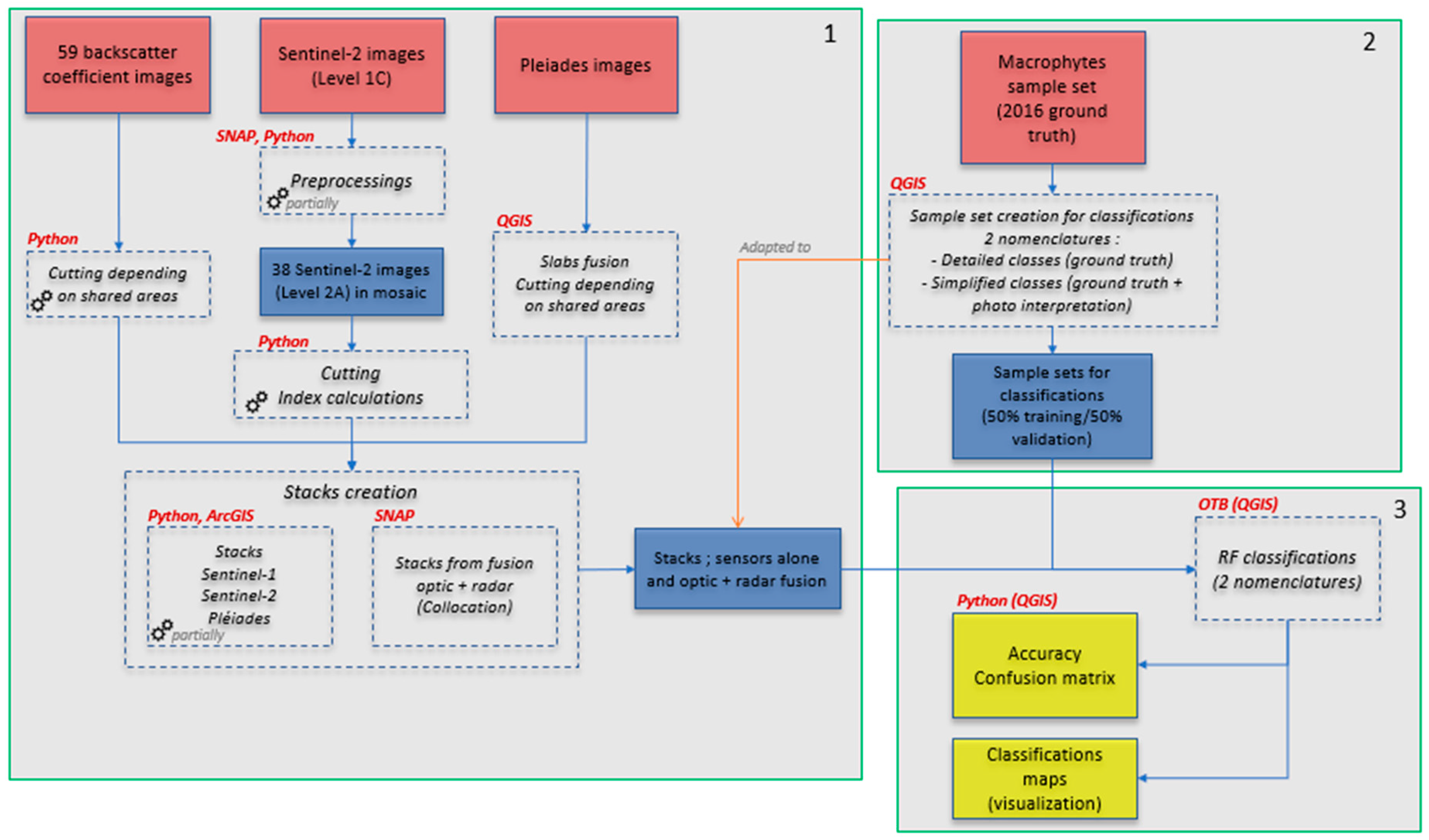
2.3.2. Machine Learning Method (Random Forest) and Classification of Macrophytes

The second section entailed identification and and mapping of Phragmites australis and other aquatic macrophytes (submerged, emergent, floating-leaved, etc.) from optical images (S2 and Pleiades) and radar images (S1) (Figure 4).
To compare the different classifications with each other, we chose the same two areas for each sensor (Figure 2). As Pleiades had the smallest number of satellite images, we used it to choose areas. These areas were then cross-referenced based on locations where there were field surveys. The northern zone of classification corresponds to the lakes whose field samples were made from 25 to 26 July 2016 and the south to those made from 17 to 19 May 2016. For the radar data to be included in the classifications, the backscattering coefficient was preferred to the coherence because it corresponds to a single date and not to a comparison of two dates. Moreover, the coherence images did not allow us to correctly distinguish elements on the lakes contrary to the coefficient of backscatter. For S2 data, an atmospheric correction (transition from Level 1C to Level 2A) was applied to all images via the ESA SEN2COR module. They were then resampled in SNAP to put all the bands at a resolution of 10 m, then mosaicked to get the image of the entire delta. Finally, the images have been adjusted to classifications as S1 data, by the python script. The PIR bands at 20 m (8A), water vapor (9) and cirrus (10) were not used, but that of the coastal and aerosol (1) was retained as useful for studying the shallow waters. The calculations of the eight S2 indices: enhanced vegetation index, modified chlorophyll absorption in reflectance index, normalized difference pond index, normalized difference turbidity index, normalized difference vegetation index (NDVI), normalized difference water index (NDWI), and pigment specific simple ratio (Table S3/Supplementary material) were automated in the python script.
The Pleiades images were reconstituted in QGIS, then cut to the boundaries of the classification areas, also in QGIS. Only NDVI and NDWI were calculated, to limit the weight of Pleiades stacks, and because the satellite only has visible bands and NIR. Stacks fusing optical data and radar were made with the SNAP Collocation feature, which resamples a data source to coincide with another. Here we resampled the radar according to the optical data. S1 stacks were created with 3 bands each time, VH, VV, and VH/VV. S2 stacks were created according to 3 variants; the original bands alone (10 bands), the indices alone (8 bands), and the two sets (18 bands). For Pleiades, two variants were created; the original bands alone (4 bands) and the latter with the indices (6 bands). Once all optical stacks were carried out, a version of each was fused with the corresponding radar stack. The choice to produce many diverse stacks was made to observe the separate influence of the bands, indices, and radar images in the results of the classifications.
The last step was to calculate the random forest algorithm to all stacks for the classification of aquatic macrophytes in lakes within the delta and Phragmites australis. This step was realized on the free software Orfeo ToolBox (OTB), in the version incorporated into QGIS. Random forests is a nonparametric ensemble classification and regression machine learning approach based on many decision trees as base classifiers [45,46,47]. To classify an image, it randomly selects training data and variables many times to develop numerous trees, then applies each unique set of trees to classify the image, generating a final classification that is an ensemble of multiple trees, assigning the class by majority model. The tree depth and minimum sample size are the two most important parameters in the RF classifier. In this work, the number of trees was set to 500 and the number of features in a subset was the square root of the total number of features used in this study. In order to train and validate the model on independent datasets, we randomly split the database into 50% for training and 50% for validation [48].

2.3.3. Ground Reference Data Collection

To ensure a nonbiased assessment of classification accuracy, both model training data and model validation data were collected using a sampling framework. In this study, the ground data collection step to validate the results of the supervised classifications combines two categories of survey methods, random methods (probabilistic) and empirical methods (nonrandom). Implementing a probabilistic sampling design contributes to a scientifically defensible accuracy assessment. Probabilistic sampling designs include systematic, clustered, simple random, and stratified random. Probabilistic sample methods were applied for the homogeneous thematic areas classes of macrophytes. Satellite imagery (Pleiades) served as the sampling frame for the references data. A total of 100 points in zone north and 105 points in zone south with a confidence interval of 95% were surveyed. The random survey was chosen and applied using the ENVI software.
This survey determines the membership of an observation unit in a sample based on a random draw. In this case, the probability is known. The random draw was stratified from the set of homogeneous thematic areas. The stratification was carried out before the field investigation phase. The front stratification allows a radiometric contact of the ground to set up the sampling. The stratification at this first stage is a morphological type stratification, which is based on criteria of textural homogeneity, backscattering (in the case of radar images), and then thematic homogenization. Zoning by homogeneous sector with respect to the variable studied (macrophytes) from this morphological stratification is essential. The stratification improves the precision of the accuracy and area estimates [49].
For the observation of the macrophytes, first, an empirical survey was conducted to guide the data collection phase. Sample coordinates were collected during the survey using a global positioning system (GPS). In this stage, the following aspects are achieved: the geographic position of the points, their description (the description of the vegetation is physiognomic with an estimate of the cover), and their location on the classified satellite image or on a color composite of optical images. Second, a survey by route for areas accessible only by boat was carried out (except for lakes). The routes were chosen according to the channels existing in our area of work. Along the route, the points on the grid of the random stratified survey were first observed. This survey first asks for a selection of the main elements of the plant landscape. Thus, a few typical units, representative of the vegetation units crossed, were analyzed. This survey is also known as “sample units,” according to the name of the sample of individuals. Observations by standard units were chosen by vegetation stratum [50]. Stratification was carried out on satellite documents (Pleiades) before the field mission to validate the results. The objective of this stratification is to ensure a good thematic dispersion of the sample. In general, a minimum of two units per stratum is required for this stage of field data collection. The positioning of the standard units was chosen in a station physiognomically homogeneous from a point of view of flora and plant formations. The data included floristic composition and vegetation structure, using Braun–Blanquet estimates. The description of the vegetation is physiognomic with an estimate of the cover. The size of the observation unit is more or less important depending on the size of the homogeneous area. The structure as well as the type of vegetation were noted at each point within a radius of 25 m around the observer. The information collected were: date, precise location (mapping), and total vegetation cover. Some floristic information was also recorded: list of species classified by physiognomic stratum (different classes of Phragmites australis and emergent aquatic macrophytes).
In our analyses, we used an aquatic macrophytes database from 2016 [51], that covers 43 representative lakes of the Danube Delta. The database includes 895 species records and 205 surveys. Sampling of aquatic vegetation was done by boat or canoe. The number of surveys on the lake was established according to the size of the lake. The total cover of the plants and the individual cover of the species of plants and filamentous algae were estimated visually and by harvesting with a harvesting rake. For each species, the percentage of cover was estimated using a 5-point scale according to Kohler, A. [43].

2.3.4. Accuracy Assessment

To be relevant, an accuracy assessment should meet certain requirements, such as confusion matrix normalization [52]. Indeed, after generating the raw error matrix, also called a confusion matrix, it is necessary to normalize it by the proportion of the number of control points as well as to normalize it by the proportion of the area classes obtained in the classification. Based on our validation points, we normalized the raw error matrix in order to generate common statistics such as the overall accuracy (OA), the producer accuracy (PA) and the user accuracy (UA). We assessed classification performance using these metrics for all 67 classifications.
The OA is intended to check the conformity of the classifications at a global scale for all the classes. The OA describes the proportion of total map area that has been correctly mapped. The PA is a class indicator that characterizes the omission error (PA = 1—omission) where UA is a class indicator characterizing the commission error (UA = 1—commision).
Reporting only accuracy measures such as the overall accuracy is insufficient without taking into account uncertainties. A confidence interval is very useful because it provides valuable information regarding the margin of error in estimation and gives a range of probable values for the parameter. Indeed, whatever the sampling design, uncertainties will give the confidence interval the measure allowing an objective analysis of the results. A confidence interval provides a range of values for a parameter taking into account the uncertainty of the sample-based estimate [52].
In Olofsson [52], the confusion matrix used in accuracy assessment provides information on the magnitude of the classification errors that allow for an adjustment to be made in the area estimator. In order to quantify the sampling variability of the estimated area, the confidence intervals were calculated. The calculations of the confidence intervals were automated in the python script included in QGIS.

3. Results

3.1. Sentinel-1 Radar Images to Differentiate the Different Classes of Phragmites australis

The graphs presented in this part of the results show the temporal changes in the backscattering coefficient (Figure 5) for the classes sampled (Table 2), over the period 2016–2017, compared to daily precipitation for the same period. The left curves correspond to the reed classes and the right ones to the other classes (Table 2). An average value for each sample of each class was extracted, then each of these was averaged for all dates. We thus obtained the coherence (VH and VV) and backscatter coefficient (VH, VV, and VH on VV) time series for the 11 classes of the sample set, compared on the graphs with rainfall. We identified the backscatter double bouncing (built-up areas) and volumetric (different class of reed). The identification of the backscattering increases the possibility of RF to identify the class reed.

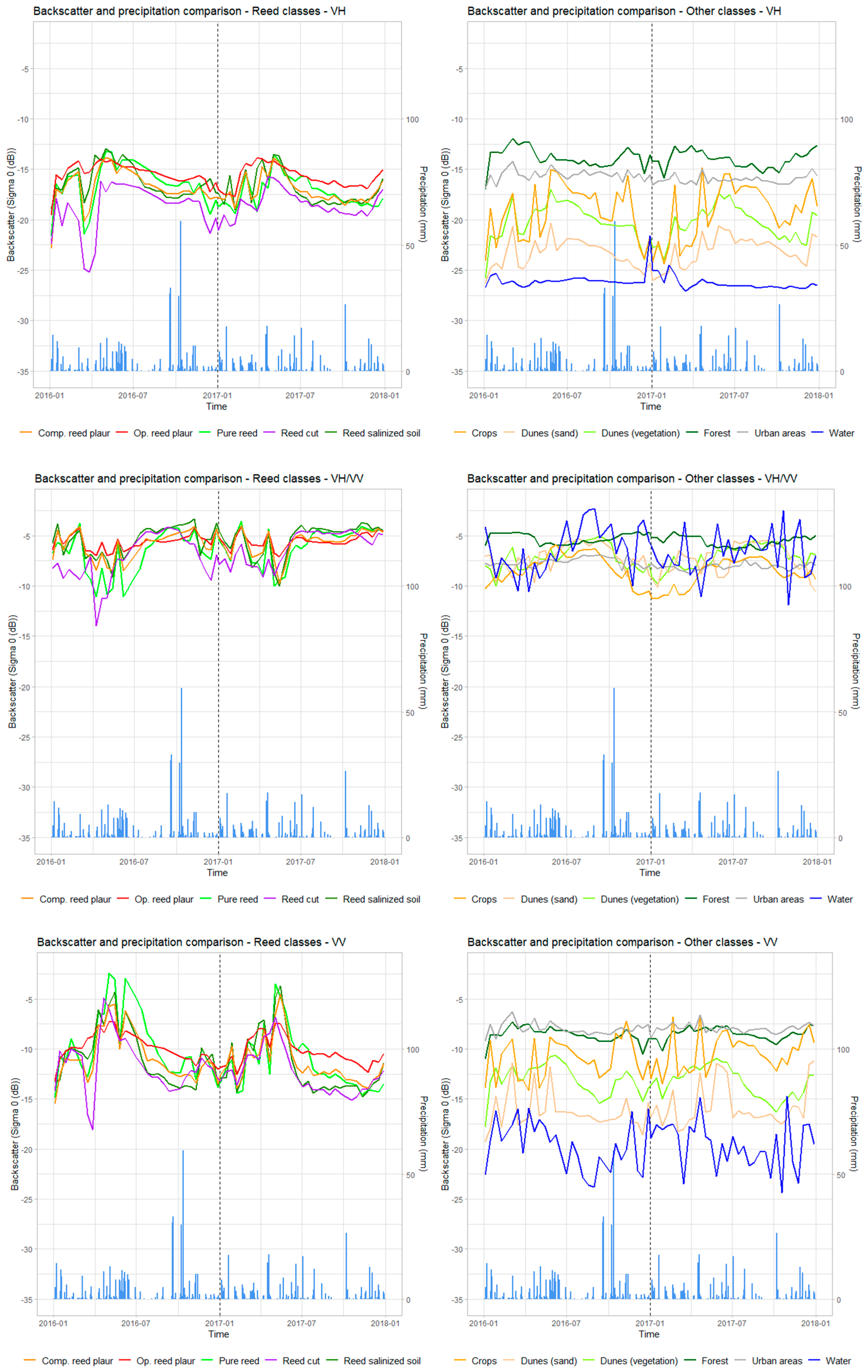
3.1.1. Backscattering Coefficient to Identify the Phragmites australis

Mean backscatter (Figure 5) varied logically between the different polarizations of the class observed. The analysis of the backscattering coefficient allowed us to provide information for separation between classes of macrophytes, some of which overlap strongly.
To interpret the backscattering, it can be recalled that the vegetation tends to return the radar signal in many directions and therefore has high values, while water and flat surfaces such as bare ground will tend to only send the signal in one direction and thus have low values. The backscatter values are lowest for VH (a), slightly higher for VV (b), and even higher for VH/VV (c). The ratio has a small amplitude compared to the other two polarizations, with values almost all between 0 and −12.5 decibels (dB). VV has the largest amplitude and shows significant backscattering peaks, especially for Phragmites australis classes. For the classes themselves we note that the different types of reed have similar curves for the 3 polarizations. On the other hand, polarizations differed between the types of reeds. VH shows an increase from January to April (about +5 dB), then a gradual decline (about −3 dB) until the end of the year, while VV shows a larger increase (about +10 to 15 dB) until April–May, then a decline of the same amplitude until the end of the year. VH/VV shows alternating small increases then decreases on the order of 2 dB, stabilizing around −5 dB after July. Between 2016 and 2017, there are two differences in behavior; the first is the sudden decrease in backscatter in March and early April 2016, visible especially for the cut grass (in purple), but also to a lesser extent for other types of reed. This variation may be related to a late cut of the reed at the beginning of the year. The second difference is the behavior of backscattering at the end of the year (November and especially December), where in 2016 fluctuations are noted (and continue in early 2017), while in 2017 there is an increase (or stagnation for VH/VV). The cut reed is the class that is the most separable from the other classes, with the weakest backscattering values and the largest annual variation. The pure reed class (light green) also stands out, with the most important VV backscattering peaks in mid-2016. For the other classes, the interpretation is simpler. In VH, as in VV, the curves do not change much. VV shows larger peaks for dunes (sand) and water. Buildings and forests have the strongest and most consistent values for VH and VV. This seems logical since it is these surfaces that retain an important geometry all year round (buildings and tree trunks). Dunes with vegetation have a very similar behavior, with slightly higher values for vegetation. Their curves showed a peak in late spring and summer, and a low in winter over the two years observed.
By visualizing the calculated images, we obtain significant results for the identification of the reed plaur and the aquatic macrophytes (Figure 6).
It is possible to follow the displacements of the plaur reed on the surface of the lakes with images of the backscattering coefficient (Figure 6, in red), in particular with the VV polarization. VH only distinguishes water surfaces, while VH/VV seems to track algal blooms for certain dates. It is also noted that these VV backscattering data make it possible to see changes in lake cover by aquatic macrophytes (Figure 6, in cyan).

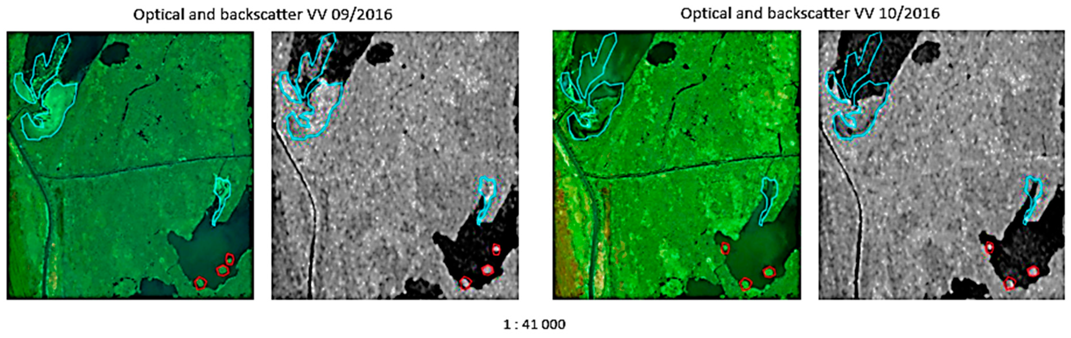
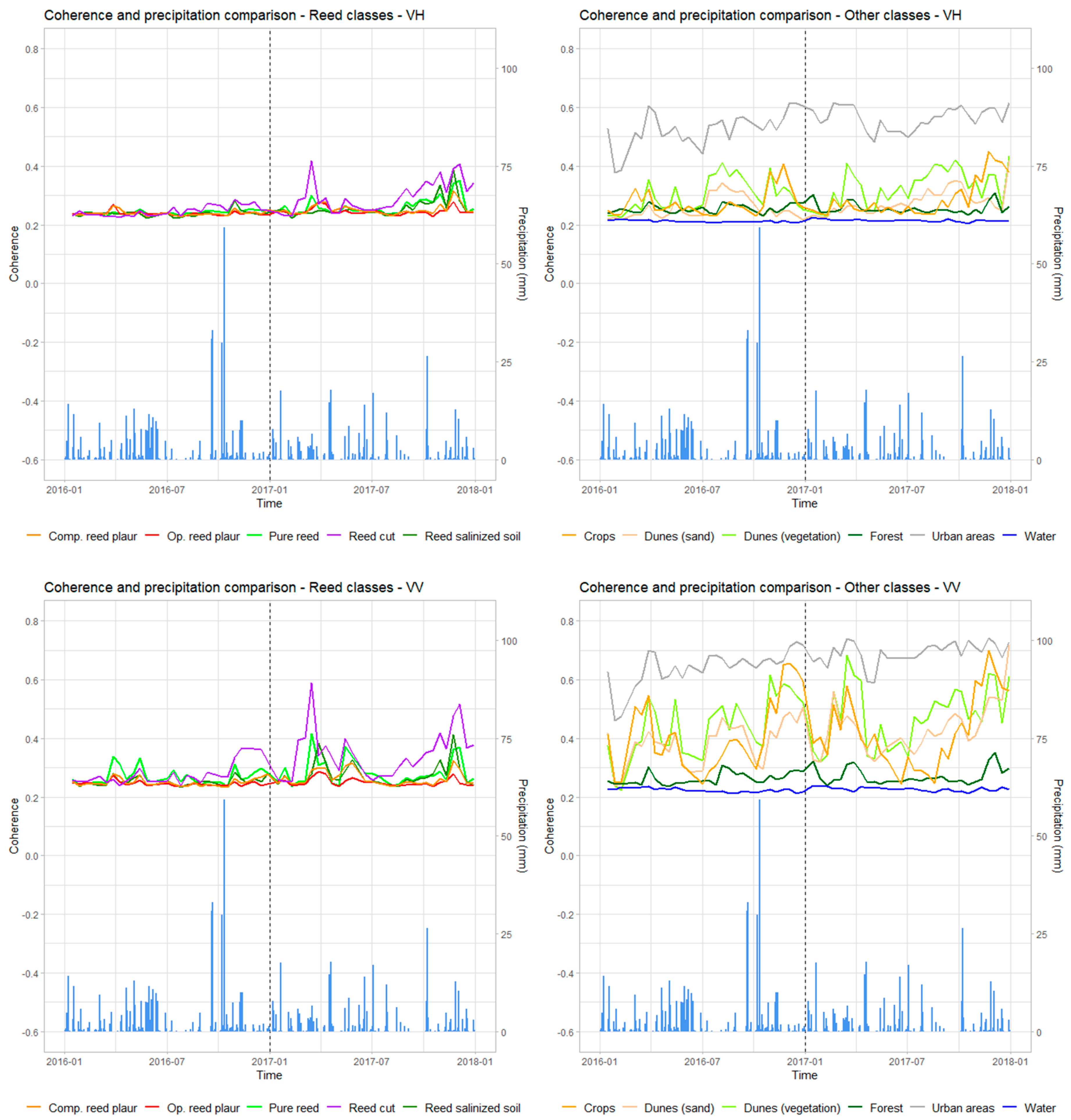
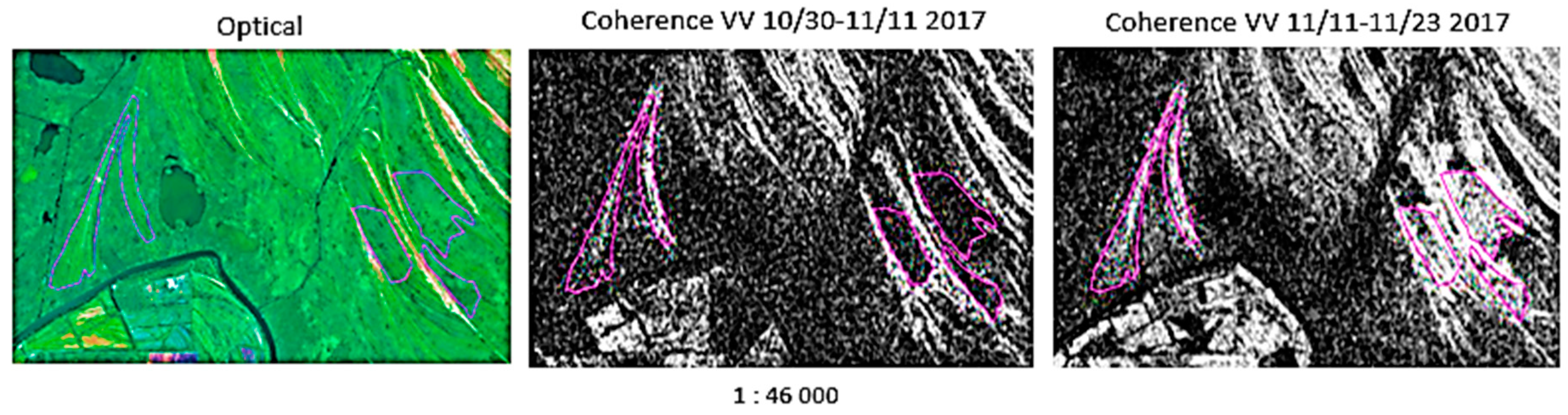
3.1.2. Coherence for the Different Classes of Phragmites australis and Identification of the Cut Reed

The interpretation of the coherence values is different from that of the backscattering coefficient. Surfaces with stable backscatter and phase such as urban or bare soils have high values. When we study vegetation with coherence, we observe the moment when it disappears to reveal the soil, resulting in an increase in values. As for the backscattering coefficient, the VV coherence shows a larger amplitude and larger peak than VH (Figure 7).
For the reed classes, there is a great similarity in the behavior of the different types, and between VH and VV as well. For both polarizations, the reeds had low values of coherence between 0.2 and 0.3 throughout the year. Some classes such as pure reed or reed on saline soil had rare peaks between 0.3 and 0.4. The cut reed is the class of reed whose coherence shows the highest values (0.42 for VH and 0.59 for VV). These increases in coherence occur at the end of the year and can therefore be linked to cutting events. Similar results can be found in cutting crops and sugar in other studies [53,54]. For the other classes, the amplitude is higher, with the frame that conserves in VH as in VV of strong values throughout the two years (between 0.38 and 0.74). The water and forest also remain fairly constant, in the low values, between 0.2 and 0.3. The forest has small increases to 0.3 or more, mainly in winter, which could be related to the loss of leaves and exposed trunks, a little more stable in their phase. This is similar to the results of another study [53]. Crops and dunes (vegetation and sand) show the most important variations in all classes. They are also more marked in VV. For crops, there are many periods of bare soil with increases in winter, partially corresponding to low backscatter values at the same time periods.
As for the backscattering coefficient, the coherence values for 2016 and 2017 do not seem to be influenced by precipitation trend. By visualizing the calculated images, we obtain significant results for the idntification of the reed cut (Figure 8).
VV coherence is the best data for monitoring the reed. In Figure 8, we can observe the appearance of strong values of coherence for several areas (in purple). The dates correspond to the cutting period, late autumn and early winter. The image is located in the center-east of the delta, an area where the reed is very exploited. The same trend of the reed surfaces is observable in November 2016 and March 2017 (for this period, the link with a reed cut is less certain). The phenomenon does not happen gradually, and we can probably date a section between 11/11 and 11/23/2017.

3.2. Macrophyte Classifications

3.2.1. Nomenclature

In this study, we used detailed nomenclature and simple nomenclature. The detailed nomenclature distinguishes macrophyte species and is based mainly on field survey records, although some classes contained very few records. For this nomenclature, it was assumed that macrophytes remained more or less at the same place in time on the lakes, since they are attached to a substrate. So we created only one set of samples per zone and one adapted to each classified date. The simple nomenclature differentiates submerged macrophytes from emergent macrophytes. Dates for satellite images were selected differently according to the nomenclature used. For the detailed nomenclature, the dates closest to the sampling date were selected for S1 and S2. For Pleiades, the date was necessarily on at 11/07/2017. On the other hand, for the simple nomenclature, which is largely dependent on the samples, the date for each zone with visibility on the lakes (no clouds, acceptable water turbidity) and the most apparent macrophytes were selected. The detailed nomenclature took up all the classes of the field samples, grouping together some of them when they were very similar (e.g., Potamogeton pectinatus and Potamogeton trichoides, or Ceratophyllum demersum and Ceratophyllum submersum L.). For the northern classification area, seven classes of macrophytes and one class of reed/other were distinguished for areas that surround the lakes, a water class, and a class of “no data”, i.e., 10 classes. For the southern classification zone, 10 classes of macrophytes and also classes of reed/other, water, and no data were taken into account, i.e., 13 classes. To create the samples of this nomenclature, we relied on field samples, especially because the species were not visually distinguishable to create them by photo-interpretation, especially on S2. For this reason, two sets of samples (one for each zone) were created so that they were suitable for Pleiades, S2 and S1, and also for the different dates of the images used. The simplified nomenclature was created by serving classes of field samples for macrophytes that can be seen visually on the images and whose species were known precisely with field data. This was the case for two emergent species (floating, broad-leaved), Nuphar lutea or yellow water lily and Trapa natans. The rest of the species, visually indistinguishable from each other, were united in a class of submerged macrophytes. For the northern classification zone, five classes were differentiated (Nuphar lutea, submerged macrophytes, water, a class of reed/other, and a class of “no data”). For the southern zone, the same classes were differentiated, to which Trapa natans was added, as well as those of algal bloom and sediments, visible at the dates studied, i.e., height classes. With this simpler nomenclature, we were able to create more samples per class that were more extended and better distributed throughout the territory to be classified. On the other hand, as this nomenclature is based on photo-interpretation, we created a set of samples for each date. We had two sets (north and south zones) adapted to S2 (2016 images) and two adapted to Pleiades (images from 11/07/2017) or four sample sets in total. For each optical classification, the image S1 corresponding to the level of the date was classified. The sample set used was adapted according to whether the optical reference classification was on S2 or on Pleiades.

3.2.2. Estimating Overall Accuracy

Validation of the classifications was done with and without samples for the reed/other class, to highlight its influence on the results. In the Table 3, the values of OA for validation with reed class without this class.
The results following the calculations of the OA and their confidence intervals applying the RF model classifications for three sensors show the difference between classifier accuracies of various variable stacks. The detailed nomenclature overall has lower accuracies of OA compared to those using the simple nomenclature for all sensors and for all combinaisons (Table 3). Overall, the northern zone presents higher accuracy of OA for the different stacks compared to the southern zone. Systematically, accuracy of OA with samples validation reed is greater than accuracy of OA without samples validation reed (Table 3).
For classifications using the detailed nomenclature, the highest accuracy was obtained with S2 (bands and indices) fused with S1 (as of 17/07/2016) (Table 3). The less efficient stack for obtaining high accuracy was S1 for detailed nomenclature. This is in agreement with what is found in the literature [55,56,57]. The stack S2 set and Pleiades gave very high accuracy for this nomenclature. The stack S1 was a high accuracy in the simple nomenclature (Table 3).
The first results of the classifications showed that the emergent macrophytes were well classified, except some species, in particular for the detailed nomenclature, and it seemed interesting to test the evaluation of the classifications with and without this class to see its influence. This is possible because the evaluation is done only on the pixels included in the validation samples. No validation sample was created for the “no data” class (created simply to isolate these pixels from the others), because all of its pixels were invariably well classified. At the same time, height and vegetation and water indices were included in the RF classifications. The application of optical radiometric indices is widely accepted as a means to improve classifications [55,58,59]. For the accuracy that included different optical indices in the RF classifications, we analyzed the different stacks of S2 and Pleiades. Regarding the test of the different stacks for optical images (bands, height indices, and bands and indices), the three sets provided similar accuracy, with a slight increase overall when the bands and indices were used together. For the detailed nomenclature (north zone) for the date of 07/17/2016, the eight indices had the lowest accuracy (OA: 64.21 ± 2.1), the bands an intermediate result (OA: 69.02 ± 0.02), and the bands and indices a slightly higher result (OA: 72.32 ± 3.2) (Table 3). Most of this was also observed for the other dates, for the two zones and with or without the addition of the radar, with sometimes the eight indices giving better results than the bands, but in general with the third stack giving the highest accuracy.
In conclusion, for the accuracy of OA for the detailed nomenclature in north zone, the following stack obtained accuracy greater than 90%: S1 + S2 (bands + indices) (90.31 ± 1.2) Table 3. Between 80% and 90% accuracy we had the following stacks: S2 (bands) and S1+ S2 indices. An accuracy of less than 80% was obtained for the following stacks: P + S1, S1, S1 + S2 (bands), and S2 (bands + indices)). In south zone, the situation was different: no accuracy greater than 90% for detailed nomenclature was obtained. The most efficient stack was the P + S1 with an accuracy of 78.79 ± 1.02 Table 3. Accuracy greater than 70% was obtained with the following stacks: S2 (bands), S1+ S2 indices , and S1 + S2 (bands). In the case of simple nomenclature, all the stacks used presented very high accuracy (greater than 90%) for the northern zone. The most efficient stack with very high accuracy was P + S2 (indices) + S1 (98.15 ± 0.02) Table 3. Other stacks with notable accuracy higher than 95% were: P + S2 (indices), S1 + S2 (bands + indices), S2 indices, and S1 + S2 (bands). In the south zone, the most efficient stacks were S1 + S2 (bands + indices) (98.53 ± 0.08) and S2 indices (98.18 ± 0.14) Table 3. Other stacks have obtained high accuracy, higher than 90%: P + S2 (indices) + S1, S1 + S2 indices, and P + S2 (indices).

3.2.3. Estimating Producer’s Accuracy (PA), User’s accuracy (UA)

In order to analyze in more detail the error for the different classes, we focused the analysis on class accuracy indicators (Table 4). The confidence intervals was calculated at 95%.
The best results were obtained for the following combinations: classification of the S2 stack (bands and indices; 07/17/2016) with S1, using detailed nomenclature; classification of the Pleiades stack (bands and indices; 07/11/2017) with S1 in simple nomenclature; classification of the Pleiades stack (bands and indices; 07/11/2017) with S1 in simple nomenclature.; classification of the S1 + S2 stack (bands and indices), 08/06/2016, in simple nomenclature; and classification of the S2 stack (bands and indices; 08/16/2016) in simple nomenclature.
The second analysis was carried out by species of macrophytes. The best results are presented in the table (Table 5).
The Phragmites australis is distinguished in all combinations in comparison with other macrophytes in the two nomenclatures. All stacks presented UA and PA higher than 90%. Some stacks presented maximum accuracy (100%) for the two parameters: with detailed nomenclature: S1 + S2 (indices) and S1, S2 (bands) in the north zone. In the case of simple nomenclature, S2 (bands) had the maximum accuracy in the north zone. In simple nomenclature, other stacks presented accuracy (UA and PA) close to the maximum values: S2 (indices) (99.91 ± 0.06 and 99.62 ± 0.11) and P + S1 (99.52 ± 0.01 and 99.01 ± 0.01) Table 5 in the north zone. In the south zone, the following stack had high accuracy: S2 (indices) (99.89 ± 0.02 and 99.72 ± 0.1), S1 + S2 (99.50 ± 0.06 and 99.99 ± 0.02), and P + S1 (99.43 ± 0.01 and 97.81 ± 0.01) (Table 5).
The aquatic macrophyte Nuphar lutea had a very high accuracy (100%) for PA and UA in detailed nomenclature for the north zone for the following stacks: S1 + S2 and S2 (bands). The stack P + S2 (indices) had a very high accuracy too for the two parameters (Table 5). In simple nomenclature, four stacks were performing with accuracy greater than 90%: S1 + S2 (in north zone) and S2 (bands + indices), S2 (bands), and S1 + S2 (in south zone). The submerged macrophytes give the highest accuracy for the north zone. Some stacks had a maximum accuracy for the detailed nomenclature: S1 + S2, S2 (bands) and S2 (bands + indices). Ceratophyllum sp. had a very high accuracy only in the north zone for the detailed nomenclature: S1 + S2 (100% and 100%). The stack P + S1 was detected at high accuracy (99.86% ± 0.26 and 99.49% ± 0.35). Trapa natans was detected at high accuracy only in south zone with the simple nomenclature in S1 + S2 indices.
Most macrophyte species were identified with good accuracy with the stack S1 + S2 indices except for the Myriophyllum spicatum with minimum accuracy for the two parameters (0.0% ± 0.0 and 0.0% ± 0.0) (Table 5). The same accuracy was found for the same macrophyte for all dates of the stack S1 for the north zone. Vallisneria sp. presented the same results for stack S1 for the north zone. In the south zone, the same accuracy (0.0% ± 0.0 and 0.0% ± 0.0) was found for Elodea nuttallii (Planch.) H.St.John, in the stack S1+ S2 (bands and indices) with the detailed nomenclature.

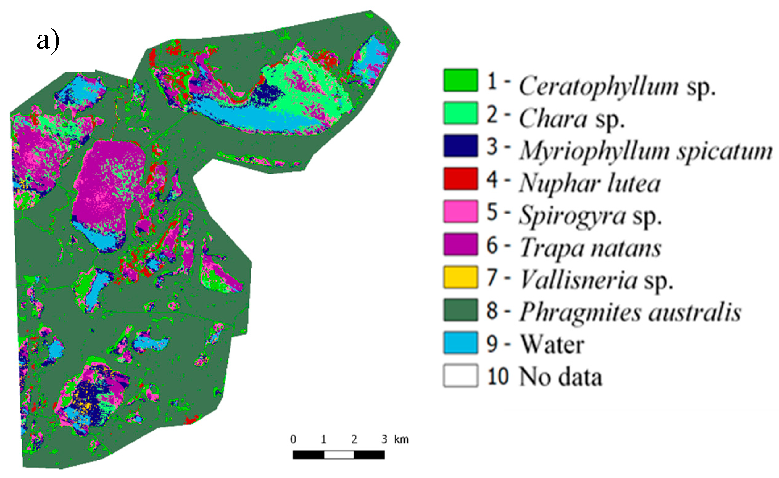
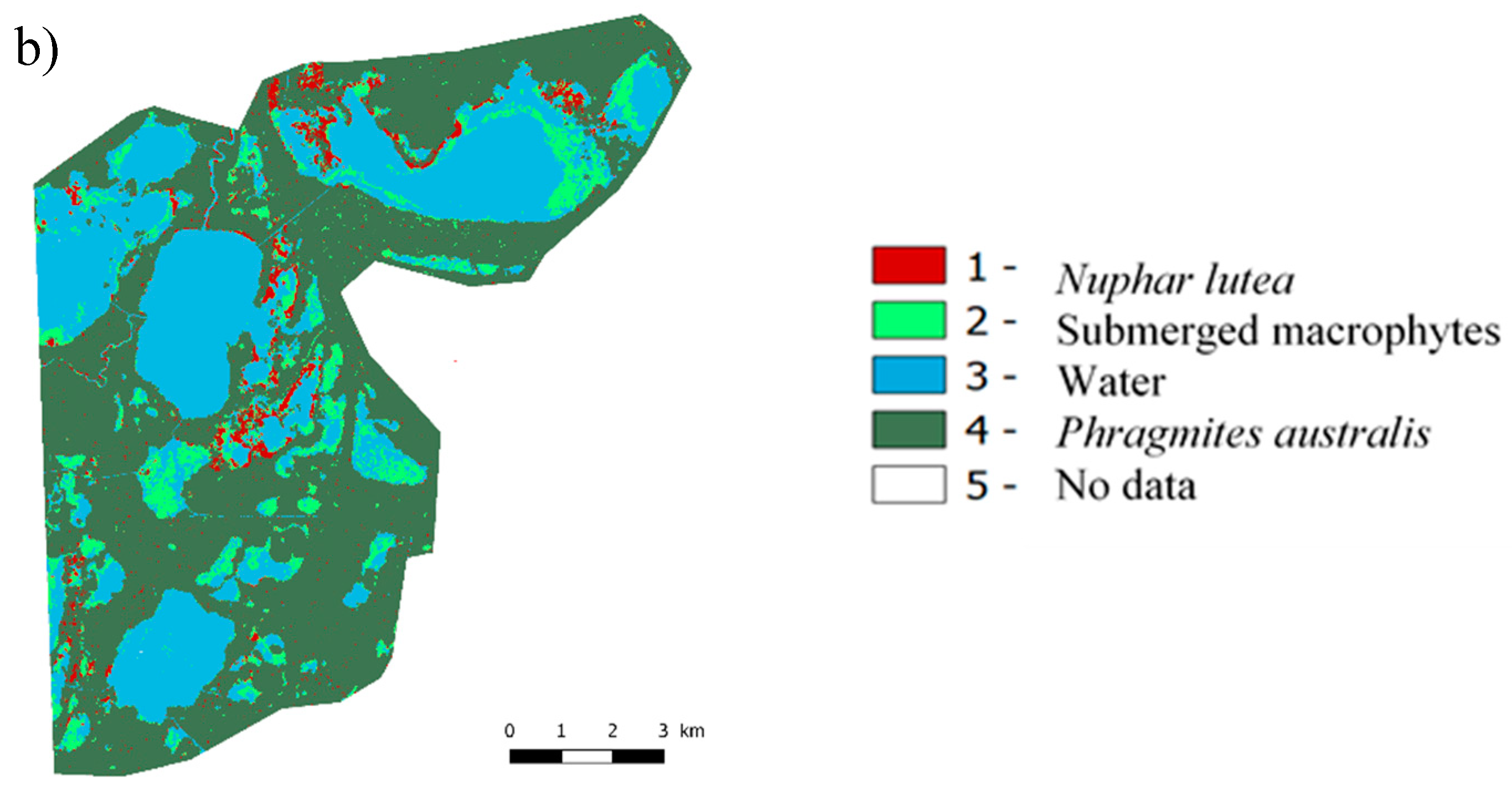
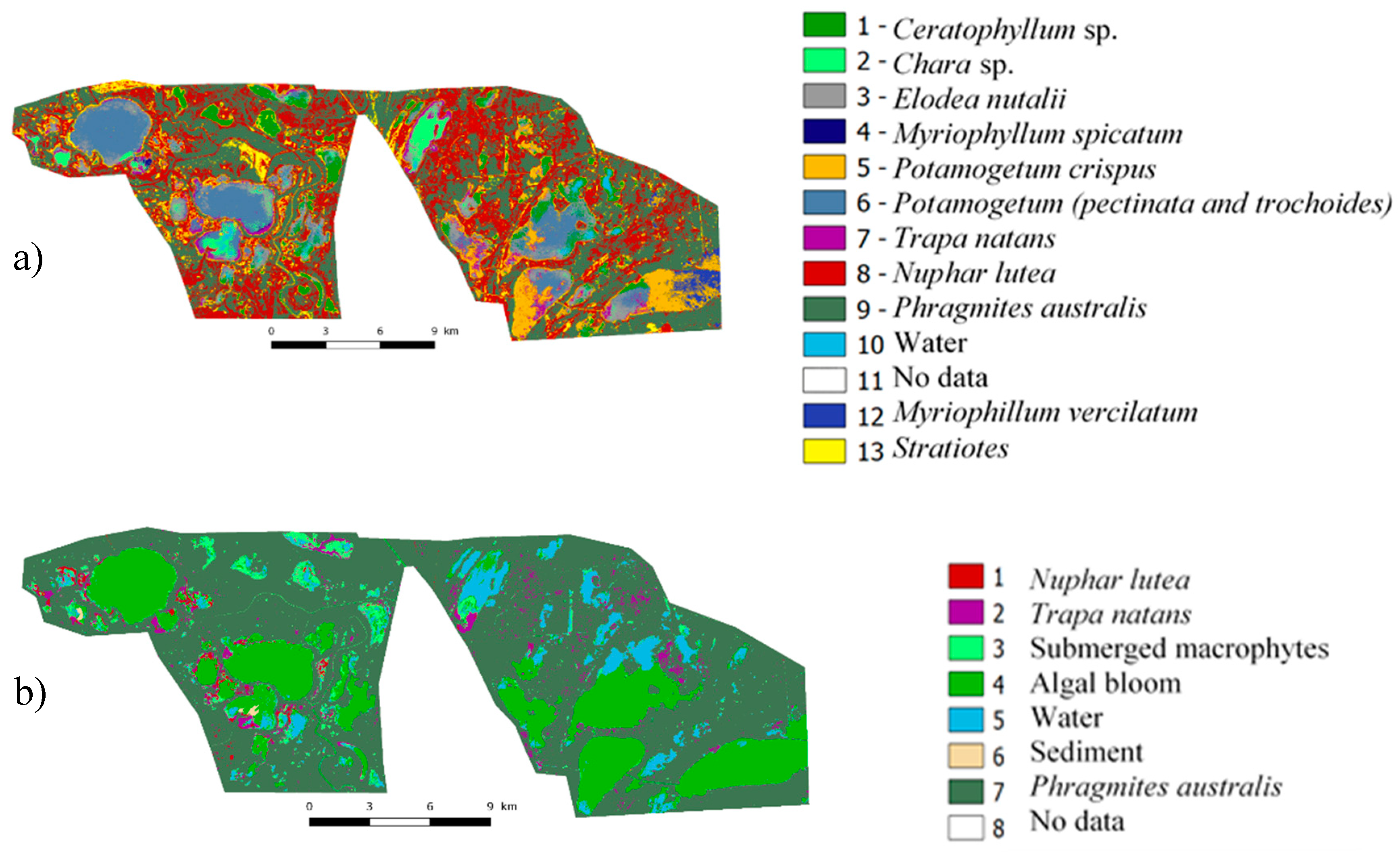
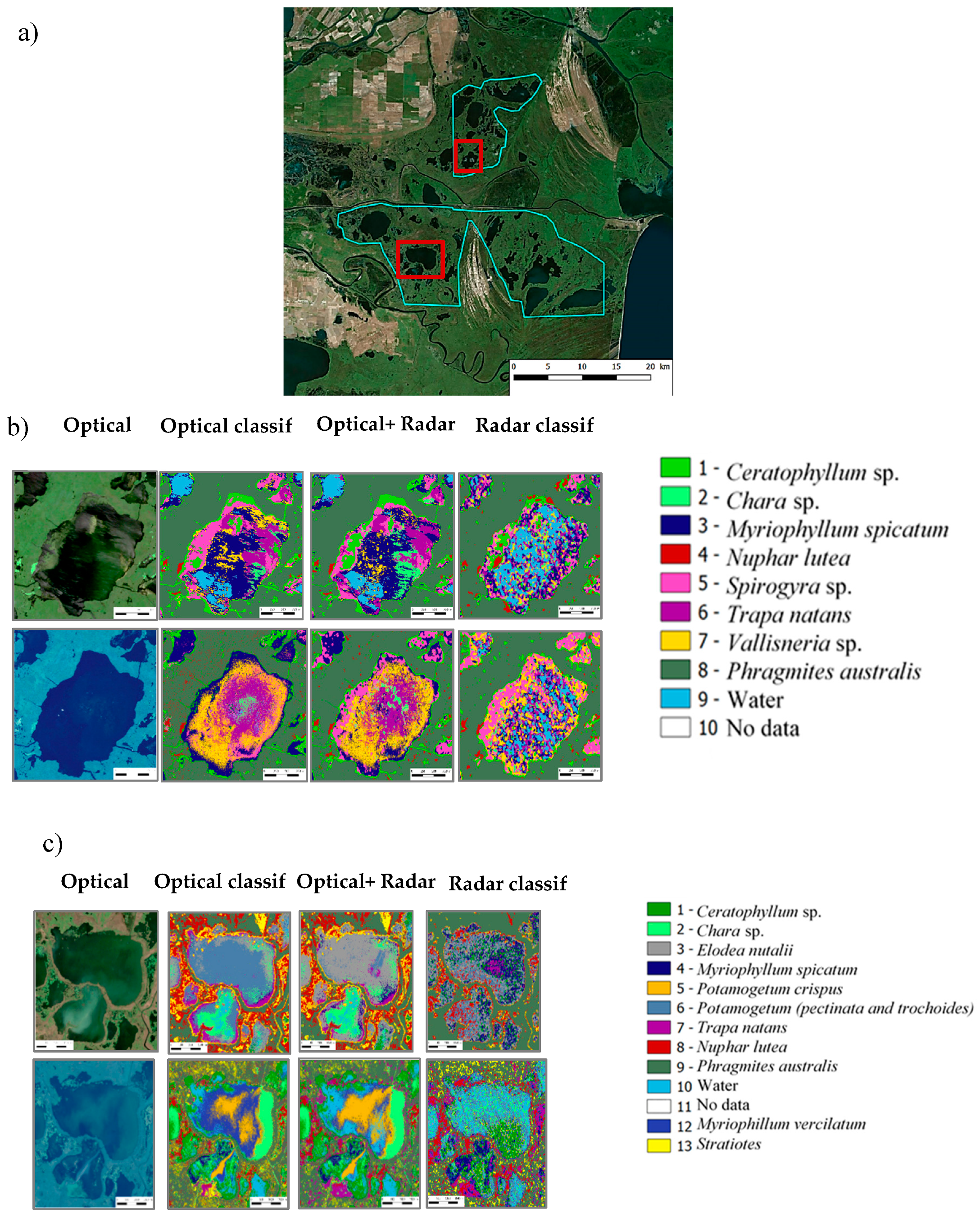
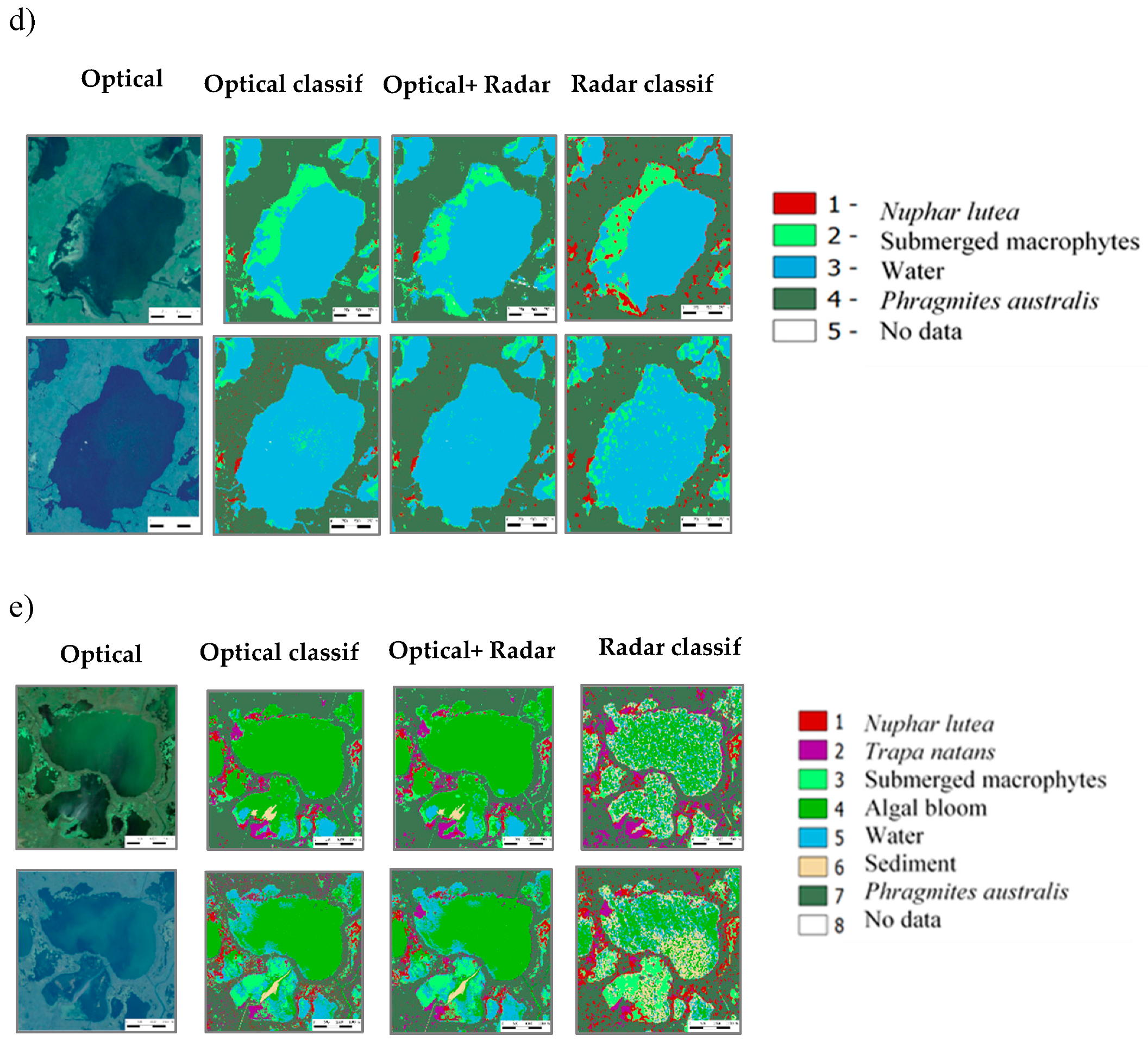
3.2.4. Mapping Macrophytes

The classifications derived from the precise nomenclature were more complex to interpret, and their classes were much more mixed. For that of the northern zone (Figure 9), many different classes of aquatic macrophytes were found on the same lake, and for that of the southern zone (Figure 10), the Nuphar lutea and Stratiotes aloides L. classes were strongly confused with the reed class. Classifications in simple nomenclature were easier to analyze. There seems to be little confusion between classes, and the reed was well separated from other classes.
There was a big difference between the S2 and Pleiades results for the distribution of the detected classes between the north and the south zone. The species of macrophytes were not the same. For example, for the north zone, Pleiades detect a lot of Vallisneria sp., where S2 rather detects Myriophyllum spicatum, Spirogyra sp., and water (Figure 7 and Figure 8). Conversely, the classifications of the simple nomenclature showed a concordance of the Pléiades and S2 results. As for the detailed nomenclature, their dates were not the same, but the common elements visible on the true color images were found on the classifications of the two sensors. This was true for the reed or for the species Nuphar lutea and Trapa natans in particular (Figure 11b–e).
To better illustrate these classfications we show an enlarged image of two lakes in the two zones (Figure 11a).

4. Discussion

4.1. Sentinel-1 Radar Images Identified the Different Classes of Phragmites australis

In the first section, the results showing time series of backscattering and coherence coefficients captured the phenology of the main classes of Phragmites australis, or the period of cut for this macrophyte. The vegetation’s phenological cycle helped the separation of different types of Phragmites australis in the multi-seasonal approach. The increase and then the stability of the reed class values from June to November/December for VH/VV correspond to the phenology of the species. These results provide an additional argument for enhancing the correlation between phenology of the species and observation of the backscattering coefficient. Precipitation does not influence the backscatter of the different classes. Even unusual rain events do not correspond to sudden changes in backscatter. It can be hypothesized that this is due to the very wet character of the delta, which means that precipitation does not change moisture on surfaces. Finally, the vegetation phenological cycle helped differentiate the different types of Phragmites australis in a multi-seasonal approach.
Using the identification of the multi-seasonal backscattering increases the possibility of RF to identify the reed. The results agree with the results of other research [28,60,61,62]. This study demonstrates the large potential of microwave coefficients for identification of the several classes of Phragmites australis and their phenology. The coherence coefficient shows that C-band SAR repeat pass interferometric coherence for cut reed detection is feasible. Sentinel-1 data with high spatial resolution are useful for monitoring the reed cut when acquisition dates surround the cut date. The interpretation of the images shows that the difference between the coherence coefficient of the mature reed and the cut reed is very pronounced. Low values of coefficient of coherence are observed at periods when the reed is generally cut off and therefore one can know more or less precisely when they have occurred. The results also showed that the radar signal could be very independent of precipitations, taking into account that the environment is very wet by its nature.

4.2. Macrophyte Classifications

Various tests to compare results using different RF input parameters and data types were conducted. The RF approach provides relatively good accuracy without the danger of overfitting. The random forest classifier has less difficulty in simply differentiating between emergent macrophytes and submerged macrophytes than differentiating between species.

4.2.1. Accuracy Assessment

When sensor combinations were compared, OA, PA, and UA showed that a synergistic use of S1 and S2/Pleiades produced higher accuracies than use of SAR alone in most of the cases. The stack S1 alone could have high accuracy, for example in simple nomenclature (OA: 94.57 ± 0.26). The stack in combination with the radar increased accuracy for Pleiades and S2, and especially for the detailed nomenclature. For simple nomenclature, this trend was less apparent; the results that included the radar changed little (+/− 1% or 2% in most cases). Only Pleiades showed an increase with the radar in this nomenclature, especially for the southern zone (97.94 ± 0.01). Pleiades has a finer spatial resolution compared to Sentinel-2 (Tables S1 and S2/Supplementary material). It was assumed that for species analysis of macrophytes, this sensor could be very useful. But ultimately, the results with S2 demonstrated that it is possible to distinguish most of the macrophytes observed. Our study shows that the Pleiades images provide more information than the S2 in wetlands when only this sensor is used. In combination with other sensors, such as the S1, Pleiades gave very good accuracy for discrimination and mapping of the macrophytes.
The results show that classifications with simple nomenclature have stable classes, often between 90% and 100% OA for both types of sensors, except for certain classifications with only S1. This was not the case, however, for classifications with detailed nomenclature. We observed that the macrophyte and water classes are often confused. This is particularly true for the Pleiades classifications because this sensor’s finer spatial resolution has more pixels included in the validation samples than for S2 and S1. Only the reed and water classes appear stable with high accuracy. It is difficult to find particular trends for the other classes in this detailed nomenclature, except for lower overall values for S1 than for optical sensors. For the simple nomenclature, there is much less confusion of macrophytes with water. There is more confusion between the emergent macrophytes themselves (classes of Nuphar lutea, Trapa natans, and reed), even if it remains in small proportions.
The second accuracy analysis was carried out by species of macrophytes. The optical integration with radar and the optical-only classifiers stand out with generally good results of PA and UA. The accuracies increased by as much as 10% when radar and optical data were fused. However, the stack S1 showed that the radar S1 was able to identify Phragmites australis with the maximum UA and PA (100% and 100%). However, the reed was completely discriminated from the other macrophytes in all combinations and for all sensors. In all cases, the PA and PU for Phragmites australis for the north zone and with the detailed nomenclature had values over 95%. For this species of macrophyte, the very good accuracy for the PA and UA and its confidence interval was namely for the Sentinel sensors in different combinations and for the north zone. Pleiades had good results in combination with S1 in the simple nomenclature and in both zones.

4.2.2. Comparison to Other Studies

Our results agree with Whyte et al. [55], except that we have obtained good results for most macrophytes with optical data in fusion with radar data. Whyte et al. [55] applied RF and SVM algorithms for wetland classification using S-1 and S-2. In their article, using the RF algorithm, 15 classes were selected, and the best results were achieved using all products (S-1, S-2, and their derivatives). The OA was 83.3% and the Kappa coefficient was 0.72. All fusion scenarios showed higher results than using optical data only. Tian et al. [35], studying wetlands in China, applied RF classification for the retrieval of wetland land cover in arid regions by fusing Pleiade-1B data with multi-date Landsat-8 data; in our study the Pleiades data produced very high accuracies (99.87% ± 0.26 and 99.49% ± 0.35) for some species of aquatic macrophytes on the Danube Delta when fused with S1 data. In Tian et al. [35], the RF classifier achieved an overall accuracy of 93% and a Kappa coefficient of 0.92. The same nonparametric (RF) classifier was used in the work of Dubeau et al. [63], where they used a combination of dry and wet season data to study wetlands in Ethiopia. In this study, the fusion of optical and radar data was proposed. This combination of multispectral optical, radar, and topographic variables provided the best overall classification accuracy, 94.4% and 92.9% for the dry and wet season, respectively. Spectral and topographic data (radar data excluded) performed nearly as well, while accuracies using only radar and topographic data were 82–89%. In our study, the radar only (S1) gave modest results in comparison with the optical radar synergy, but for Phragmites australis, the radar (S1) had the highest precision for the areas studied and for the dates available. Fu et al. [34] used optical and radar fusion to study wetland vegetation. Comparison of six classification scenarios indicates that the use of additional multi-source data sets achieved higher classification accuracy. In this work, object-based and pixel-based RF classifications both achieved greater than 80% overall accuracy for both GF-1 and GF-1 (Chinese Gaofen-1) fused with SAR images (L-band PALSAR and C-band Radarsat-2). In our study, the synergy of optical and radar data (S1, S2, and Pleiades) for most of the species of macrophytes indicates higher classification accuracy. In other studies on the vegetation of wetlands (Selenga River Delta of Lake Baikal, Russia), Lane et al. [64] have proposed 22 classes of aquatic and wetland habitats. They explored and evaluated the utility of an eight-band satellite system (Worldview-2). Their OA accuracy was 86.5% (Kappa coefficient: 0.85). In our work, we used a maximum of 13 class of macrophytes including the reed, but we used the SAR in synergy with two optical sensors, and the diverse accuracy was greater than the OA of study of Lane et al. [64].

4.3. Future Directions

Optical and infrared indices have limitations associated with opacity of the atmosphere due to clouds, water vapor, and aerosols. It is known also that vegetation indices developed in optical remote sensing can only provide information on the surface of the canopy. NDVI and leaf area index (LAI), for example, are correlated with the amount of plant biomass to a certain limit. Radar remote sensing can overcome some of these limitations given the ability to work with multiple data configurations (multi-temporal, multi-frequency, multi-polarization, and multi-angle). With a frequency, an angle of incidence, and if the polarization signal is adequate, the radar signal can interact better with the canopy and provide volumetric information about the vegetation. At low frequency, the radar signal can more or less penetrate thick canopies and provide information on the total amount of biomass available. The radar vegetation index, as first introduced by Kim and van Zyl, (2004) [65], is a measure of volume scattering (from randomly oriented dipoles), a scattering mechanism usually caused by complex structural elements of vegetation (e.g., combination of leaves, branches, and trunks). In this context, some future research can be planned: a comparative analysis of the radar indices, namely the radar vegetation index (RVI) and the dual polarized radar vegetation index (IVRDvv) in two frequencies (C and X) and the difference vegetation index standard (NDVI) used in optical multispectral remote sensing in deltaic environments.

5. Conclusions

Wetlands are complex systems with the presence of lakes, channels, and several natural ecosystems more or less saturated by water that favor development of specific plant communities. Mapping, identification, and classification of wetland macrophytes using remote sensing are important because this data provide many beneficial services in planning, restoring, and managing wetlands. S2, Pleiades, and C-band dual-polarimetric SAR of S1 were deemed suitable in this study for identification and mapping of wetland macrophytes. This study showed that the chosen methodology is good for mapping the wetland macrophytes with freely available spatial data at a good temporal resolution, due to addition of the S1, S2, and Pleiades.
Random forest was applied to the S2, Pleiades, and S1 data and in situ observations for discrimination and mapping of reed against submerged aquatic vegetation (SAV), emergent macrophytes, some floating broad-leaved plants communities, and floating vegetation of delta lakes. A total of 67 classifications models, in several combinations, with two series of validation samples (with the reed and without reed) were run. The results showed that reed is completely discriminable in comparison to other macrophyte communities with all sensor combinations. In all combinations, the producer’s accuracy (PA) and user’s accuracy (UA) for the reed with both nomenclatures were over 90%. These diverse combinations of sensors were valuable for improving the overall classification accuracy of all communities of aquatic macrophytes, except Myriophyllum spicatum L.
These research findings can contribute to current knowledge of mapping macrophyte distributions since the methodology applied produces more accurate local data. The classification procedures produced from the S1, S2, and Pleiades images are reproducible, which allows their implementation on another wetlands. The maps produced are of interest to highlight habitat distribution between wetland sectors and for the assessment of ecological status of the water bodies by showing location of the aquatic macrophyte indicator species.

Supplementary Materials

The following are available online at https://0-www-mdpi-com.brum.beds.ac.uk/2072-4292/12/14/2188/s1, Table S1: Pleiades images: Bands, wavelengths, and spatial resolution; Table S2: Sentinel-2 images: Bands, wavelengths, and spatial resolution; Table S3: Different indices used for classifications.

Author Contributions

S.N. developed the concept of this study, reviewed the literature, collected in situ samples, and wrote the majority of this paper with J.-B.B. J.-B.B. designed and prepared all figures. C.L., J.H. provided written input and feedback on the content of this manuscript during the revision, D.R. provided written input and feedback on the content of this manuscript during the revision. J.H., M.D. and A.C. collected in situ samples and provided input on analysis of results. A.B. contributed analysis tools. All authors have read and agreed to the published version of the manuscript.

Funding

“This work was supported by the Centre national d’études spatiales (CNES). It is based on observations with Pleiades. This work was supported by a grant of the Romanian National Authority for Scientific Research and Innovation, CCCDI–UEFISCDI, by the Contract no. 41N/2019-Foundation of measures for ecological reconstruction of lakes in the Danube Delta based on the study of the dynamics of aquatic macrophyte habitats.

Conflicts of Interest

The authors declare no conflict of interest.

References

  1. Mitsch, W.J.; Gosselink, J.G. Wetlands; Van Nostrand Reinhold: New York, NY, USA, 1986; 722p. [Google Scholar]
  2. Van der Putten, W.H. Die back of Phragmites australis in European wetlands: An overview of the European Research Programme on reed die-back and progression (1993–1994). Aquat. Bot. 1997, 59, 263–275. [Google Scholar] [CrossRef]
  3. RejmánkováJ, E. The role of macrophytes in wetland ecosystems. Ecol. Field Biol. 2011, 34, 333–345. [Google Scholar]
  4. Casanova, M.T. Using water plant functional groups to investigate environmental water requirements. Freshw. Biol. 2011, 56, 2637–2652. [Google Scholar] [CrossRef]
  5. Taddeo, S.; Dronova, I.; Depsky, N. Spectral vegetation indices of wetland greenness: Responses to vegetation structure, composition, and spatial distribution. Remote Sens. Environ. 2019, 234, 111467. [Google Scholar] [CrossRef]
  6. Jensen, D.; Cavanaugh, K.C.; Simard, M.; Okin, G.S.; Castaneda-Moya, E.; McCall, A.; Twilley, R.R. Integrating imaging spectrometer and synthetic aperture radar data for estimating wetland vegetation aboveground biomass in coastal louisiana. Remote Sens. 2019, 11, 2533. [Google Scholar] [CrossRef] [Green Version]
  7. Van Deventer, H.; Cho, M.A.; Mutanga, O. Multi-season RapidEye imagery improves the classification of wetland and dryland communities in a subtropical coastal region. ISPRS-J. Photogramm. Remote Sens. 2019, 157, 171–187. [Google Scholar] [CrossRef]
  8. Rapinel, S.; Fabre, E.; Dufour, S.; Arvor, D.; Mony, C.; Hubert-Moy, L. Mapping potential, existing and efficient wetlands using free remote sensing data. J. Environ. Manag. 2019, 247, 829–839. [Google Scholar] [CrossRef]
  9. Rupasinghe, P.A.; Chow-Fraser, P. Identification of most spectrally distinguishable phenological stage of invasive Phramites australis in Lake Erie wetlands (Canada) for accurate mapping using multispectral satellite imagery. Wetl. Ecol. Manag. 2019, 27, 513–538. [Google Scholar] [CrossRef]
  10. Abeysinghe, T.; Milas, A.S.; Arend, K.; Hohman, B.; Reil, P.; Gregory, A.; Vazquez-Ortega, A. Mapping invasive phragmites australis in the old woman creek estuary using UAV remote sensing and machine learning classifiers. Remote Sens. 2019, 11, 1380. [Google Scholar] [CrossRef] [Green Version]
  11. Wang, H.; Ma, M. Impacts of climate change and anthropogenic activities on the ecological restoration of wetlands in the arid regions of china. Energies 2016, 9, 166. [Google Scholar] [CrossRef] [Green Version]
  12. Niculescu, S.; Billey, A.; Talab Ou Ali, H. Random Forest Classification using Sentinel-1 and Sentinel-2 series for vegetation monitoring in the Pays de Brest (France). SPIE DIGITAL LIBRARY SPIE Remote Sens. 2018, 10783, 1078305. [Google Scholar] [CrossRef]
  13. Guo, M.; Li, J.; Sheng, C.; Xu, J.; Wu, L. A review of wetland remote sensing. Sensors (Basel) 2017, 17, 777. [Google Scholar] [CrossRef] [PubMed] [Green Version]
  14. Nguyen, T.T.H.; De Bie, C.A.J.M.; Ali, A.; Smaling, E.M.A.; Chu, T.H. Mapping the irrigated rice cropping patterns of the Mekong Delta, Vietnam, through hyper-temporal SPOT NDVI image analysis. Int. J. Remote Sens. 2012, 33, 415–434. [Google Scholar] [CrossRef]
  15. Gonzalez, E.; Gonzalez Trilla, G.; San Martin, L.; Grimson, R.; Kandus, P. Vegetation patterns in a South American coastal wetland using high-resolution imagery. J. Maps 2019, 15, 642–650. [Google Scholar] [CrossRef] [Green Version]
  16. Proenca, B.; Frappart, F.; Lubac, B.; Marieu, V.; Ygorra, B.; Bombrun, L.; Michalet, R.; Sottolichio, A. Potential of High-Resolution Pleiades Imagery to Monitor Salt Marsh Evolution After Spartina Invasion. Remote Sens. 2019, 11, 968. [Google Scholar] [CrossRef] [Green Version]
  17. McCarthy, M.J.; Radabaugh, K.R.; Moyer, R.P.; Muller-Karger, F.E. Enabling efficient, large-scale high-spatial resolution wetland mapping using satellites. Remote Sens. Environ. 2018, 208, 189–201. [Google Scholar] [CrossRef]
  18. Schmidt, K.S.; Skidmore, A.K. Spectral discrimination of vegetation types in a coastal wetland. Remote Sens. Environ. 2003, 85, 92–108. [Google Scholar] [CrossRef]
  19. Silva, T.S.F.; Costa, M.P.F.; Melack, J.M.; Novo, E.M.L.M. Remote sensing of aquatic vegetation: Theory and applications. Environ. Monit. Assess. 2008, 140, 131–145. [Google Scholar] [CrossRef]
  20. Morandeira, N.S.; Grings, F.; Facchinetti, C.; Kandus, P. Mapping plant functional types in floodplain wetlands: An analysis of C-band polarimetric SAR data from RADARSAT-2. Remote Sens. 2016, 8, 174. [Google Scholar] [CrossRef] [Green Version]
  21. Adam, E.; Mutanga, O.; Rugege, D. Multispectral and hyperspectral remote sensing for identification and mapping of wetland vegetation: A review. Wetl. Ecol. Manag. 2010, 18, 281–296. [Google Scholar] [CrossRef]
  22. Zomer, R.; Trabucco, A.; Ustin, S. Building spectral libraries for wetlands land cover classification and hyperspectral remote sensing. J. Environ. Manag. 2009, 90, 2170–2177. [Google Scholar] [CrossRef] [PubMed]
  23. Ozesmi, S.L.; Bauer, M.E. Satellite remote sensing of wetlands. Wetl. Ecol. Manag. 2002, 10, 381–402. [Google Scholar] [CrossRef]
  24. Henderson, F.M.; Lewis, A.J. Radar detection of wetland ecosystems: A review. Int. J. Remote Sens. 2008, 29, 5809–5835. [Google Scholar] [CrossRef]
  25. Martinis, S.; Kuenzer, C.; Wendleder, A.; Huth, J.; Twele, A.; Roth, A.; Dech, S. Comparing four operational SAR-based water and flood detection approaches. Int. J. Remote Sens. 2015, 36, 3519–3543. [Google Scholar] [CrossRef]
  26. White, L.; Brisco, B.; Dabboor, M.; Schmitt, A.; Pratt, A. A collection of SAR methodologies for monitoring wetlands. Remote Sens. 2015, 7, 7615–7645. [Google Scholar] [CrossRef] [Green Version]
  27. Vreugdenhil, M.; Dorigo, W.A.; Wagner, W.; De Jeu, R.A.; Hahn, S.; Van Marle, M.J. Analyzing the vegetation parameterization in the TU-Wien ASCAT soil moisture retrieval. IEEE Trans. Geosci. Remote Sens. 2016, 54, 3513–3531. [Google Scholar] [CrossRef]
  28. Ferrazzoli, P.; Paloscia, S.; Pampaloni, P.; Schiavon, G.; Solimini, D.; Coppo, P. Sensitivity of microwave measurements to vegetation biomass and soil moisture content: A case study. IEEE Trans. Geosci. Remote Sens. 1992, 30, 750–756. [Google Scholar] [CrossRef]
  29. Paloscia, S.; Macelloni, G.; Pampaloni, P.; Sigismondi, S. The potential of C- and L-band SAR in estimating vegetation biomass: The ERS-1 and JERS-1 experiments. IEEE Trans. Geosci. Remote Sens. 1999, 37, 2107–2110. [Google Scholar] [CrossRef]
  30. Pope, K.O.; Rejmankova, E.; Paris, J.F.; Woodruff, R. Detecting seasonal flooding cycles in marshes of the Yucatán peninsula with SIR-C polarimetric radar imagery. Remote Sens. Environ. 1997, 59, 157–166. [Google Scholar] [CrossRef]
  31. Niculescu, S.; Lardeux, C.; Grigoras, I.; Hanganu, J.; David, L. Synergy between LiDAR, RADARSAT-2 and SPOT-5 images for the detection and mapping of wetland vegetation in the Danube Delta. IEEE J. Sel. Top. Appl. Earth Obs. Remote Sens. 2016, 9, 3651–3666. [Google Scholar] [CrossRef]
  32. Niculescu, S.; Lardeux, C.; Hanganu, J. Alteration and Remediation of Coastal Wetland Ecosystems in the Danube Delta: A Remote-Sensing Approach. In Coastal Research Library; Chapter 17; Springer International Publishing: Cham, Switzerland, 2017; Volume 21, pp. 513–554. [Google Scholar] [CrossRef] [Green Version]
  33. Niculescu, S.; Ienco, D.; Hanganu, J. Application of Deep Learning of multi-temporal Sentinel-1 images for the classification of coastal vegetation zone of the Danube Delta. Int. Arch. Photogramm. Remote Sens. Spat. Inf. Sci. 2018, 42, 1311–1318. [Google Scholar] [CrossRef] [Green Version]
  34. Fu, B.; Wang, Y.; Campbell, A.; Li, Y.; Zhang, B.; Yin, S.; Xing, Z.; Jin, X. Comparison of object-based and pixel-based Random Forest algorithm for wetland vegetation mapping using high spatial resolution GF-1 and SAR data. Ecol. Indic. 2017, 73, 105–117. [Google Scholar] [CrossRef]
  35. Tian, S.; Zhang, X.; Tian, J.; Sun, Q. Random Forest Classification of Wetland Land covers from Multi-Sensor Data in the Arid Region of Xinjiang, China. Remote Sens. 2016, 8, 954. [Google Scholar] [CrossRef] [Green Version]
  36. Mutanga, O.; Adam, E.; Cho, M.A. High density biomass estimation for wetland vegetation using WorldView-2 imagery and random forest regression algorithm. Int. J Appl. Earth Obs. Geoinf. 2012, 18, 399–406. [Google Scholar] [CrossRef]
  37. Mahdianpari, M.; Salehi, B.; Mohammadimanesh, F.; Motagh, M. Random forest wetland classification using ALOS-2 L-band, RADARSAT-2 C-band, and TerraSAR-X imagery. ISPRS J. Photogramm. Remote Sens. 2017, 130, 13–31. [Google Scholar] [CrossRef]
  38. Berhane, T.M.; Lane, C.R.; Wu, Q.; Autrey, B.C.; Anenkhonov, O.A.; Chepinoga, V.V.; Liu, H. Decision-tree, rule-based, and random forest classification of high-resolution multispectral imagery for wetland mapping and inventory. Remote Sens (Basel) 2018, 10, 580. [Google Scholar] [CrossRef] [PubMed] [Green Version]
  39. Hanganu, J.; Dubyna, D.; Zhmud, E.; Grigoraş, I.; Menke, U.; Drost, H.; Ştefan, N.; Sârbu, I. Vegetation of the Biosphere Reserve Danube Delta—With Transboundary Vegetation Map on a 1:150.000 Scale, Danube Delta National Institute, Romania; Kholodny, M.G., Ed.; Institute of Botany and Danube Delta Biosphre Reserve, Ukraine and RIZA: Lelystad, The Netherlands, 2002. [Google Scholar]
  40. Oosterberg, W.; Buijse, A.D.; Coops, H.; Ibelings, B.W.; Menting, G.A.M. Ecological Gradients in the Danube Delta lakes: Present State and Man-Induced Changes; RIZA: Lelystad, The Netherlands, 2000. [Google Scholar]
  41. Vollenweider, R.A.; Kerekes, J. Eutrophication of Waters. Monitoring, Assessment and Control. Methoden der Kartierung von Flora und Vegetation von Süßwasserbiotopen. In Cooperative Programme on Monitoring of Inland Waters (Eutrophication Control); Environment Directorate OECD: Paris, France, 1982. [Google Scholar]
  42. Kohler, A. Methoden der Kartierung von Flora und Vegetation von Süßwasserbiotopen. Landschaft 1978, 10, 73–85. [Google Scholar]
  43. Hanganu, J.; Doroftei, M. Physical landscape—Danube delta reed beds. In The Biopolitics of the Danube Delta: Nature, History, Policies; Lexington Books: Lanham, MD, USA, 2016. [Google Scholar]
  44. ESA. TOPS Interferometry Tutorial; Sentinel 1 Toolbox; Array Systems Computing: 2015. Available online: http://step.esa.int/docs/tutorials/S1TBX%20TOPSAR%20Interferometry%20with%20Sentinel-1%20Tutorial_v2.pdf (accessed on 7 July 2020).
  45. Breiman, L. Random forests. Mach. Learn. 2001, 45, 5–32. [Google Scholar] [CrossRef] [Green Version]
  46. Houborg, R.; McCabe, M.F. A hybrid training approach for leaf area index estimation via cubist and random forests machine learning. ISPRS J. Photogramm. Remote Sens. 2018, 135, 173–188. [Google Scholar] [CrossRef]
  47. Belgiu, M.; Drăguţ, L. Random forest in remote sensing: A review of applications and future directions. ISPRS J. Photogramm. Remote Sens. 2016, 114, 24–31. [Google Scholar] [CrossRef]
  48. Wang, D.; Wan, B.; Qiu, P.; Su, Y.; Guo, Q.; Wu, X. Artificial mangrove species mapping using pléiades-1: An evaluation of pixel-based and object-based classifications with selected machine learning algorithms. Remote Sens. 2018, 10, 294. [Google Scholar] [CrossRef] [Green Version]
  49. Olofsson, P.; Foody, G.M.; Herold, M.; Stehman, S.V.; Woodcock, C.E.; Wulder, M.A. Good practices for estimating area and assessing accuracy of land change. Remote Sens. Environ. 2014, 148, 42–57. [Google Scholar] [CrossRef]
  50. Wulder, M.A.; White, J.C.; Magnussen, S.; McDonald, S. Validation of a largearea land cover product using purpose-acquired airborne video. Remote Sens. Environ. 2007, 106, 480–491. [Google Scholar] [CrossRef]
  51. ***, 2019 – Fundamentarea măsurilor de reconstrucție ecologică a lacurilor din Delta Dunării pe baza studiului dinamicii habitatelor de macrofite acvatice, 19 pagini. Raport Faza 4 / Decembrie/2019, al proiectului nr. PN 19 12 02 01 04 (coord. Jenică Hanganu) al contractului nr. 41N/2019/MCI, executant: INCDDD—Tulcea. România (publication in progress).
  52. Olofsson, P.; Foody, G.M.; Stehman, S.V.; Woodcock, C.E. Making better use of accuracy data in land change studies: Estimating accuracy and area and quantifying uncertainty using stratified estimation. Remote Sens. Environ. 2013, 129, 122–131. [Google Scholar] [CrossRef]
  53. Baghdadi, N.; Moinet, S.; Todoroff, P.; Cresson, R. Utilisation de l’imagerie radar Terrasar-X THRS pour le suivi de la coupe de canne à sucre à l’Ile de la Réunion. Revue Fr. Photogramm. Télédétect. 2014, 197, 63–75. [Google Scholar]
  54. Tamm, T.; Zalite, K.; Voormansik, K.; Talgre, L. Relating Sentinel-1 Interferometric Coherence to Mowing Events on Grasslands. Remote Sens. 2016, 8, 802. [Google Scholar] [CrossRef] [Green Version]
  55. Whyte, A.; Ferentinos, K.P.; Petropoulos, G.P. A new synergistic approach for monitoring wetlands using Sentinels-1 and 2 data with object-based machine learning algorithms. Environ. Model. Softw. 2018, 104, 40–54. [Google Scholar] [CrossRef] [Green Version]
  56. Clerici, N.; Valbuena Calderón, C.A.; Posada, J.M. Fusion of sentinel-1a and sentinel-2A data for land cover mapping: A case study in the lower Magdalena region, Colombia. J. Maps 2017, 13, 718–726. [Google Scholar] [CrossRef] [Green Version]
  57. Tavares, P.A.; Beltrão, N.E.S.; Guimarães, U.S.; Teodoro, A.C. Integration of Sentinel-1 and Sentinel-2 for Classification and LULC Mapping in the Urban Area of Belém, Eastern Brazilian Amazon. Sensors (Basel) 2019, 19. [Google Scholar] [CrossRef] [PubMed] [Green Version]
  58. Erinjery, J.J.; Singh, M.; Kent, R. Mapping and assessment of vegetation types in the tropical rainforests of the Western Ghats using multispectral Sentinel-2 and SAR Sentinel-1 satellite imagery. Remote Sens. Environ. 2018, 216, 345–354. [Google Scholar] [CrossRef]
  59. Chatziantoniou, A.; Petropoulos, G.P.; Psomiadis, E. Co-Orbital Sentinel 1 and 2 for LULC Mapping with Emphasis on Wetlands in a Mediterranean Setting Based on Machine Learning. Remote Sens. 2017, 9, 1259. [Google Scholar] [CrossRef] [Green Version]
  60. Frison, P.-L.; Kmiha, S.; Fruneau, B.; Soudani, K.; Dufrêne, E.; Koleck, T.; Villard, L.; Lepage, M.; Dejoux, J.-F.; Rudant, J.-P.; et al. Contribution of Sentinel-1 data for the monitoring of seasonal variations of the vegetation. MULTITEMP 2017, Bruges, Belgium. Available online: https://multitemp2017.vito.be/sites/multitemp2017.vito.be/files/1600-1-for_websitemultitemp_27jun17_plf.pdf (accessed on 7 June 2020).
  61. Talab Ou Ali, H.; Niculescu, S.; Sellin, V.; Bougault, C. Contribution of the new satellites (Sentinel-1, Sentinel-2 and SPOT-6) to the coastal vegetation monitoring in the Pays de Brest (France). In Proceedings of the SPIE, Warsaw, Poland, 2 November 2017; Volume 10421, p. 1042129. [Google Scholar]
  62. Marbouti, M.; Praks, J.; Antropov, O.; Rinne, E.; Leppäranta, M. A study of landfast ice with Sentinel-1 repeat-pass interferometry over the Baltic Sea. Remote Sens. 2017, 9, 833. [Google Scholar] [CrossRef] [Green Version]
  63. Dubeau, P.; King, D.J.; Unbushe, D.G.; Rebelo, L.-M. Mapping the Dabus Wetlands, Ethiopia, Using Random Forest Classification of Landsat, PALSAR and Topographic Data. Remote Sens. 2017, 9, 1056. [Google Scholar] [CrossRef] [Green Version]
  64. Lane, C.; Liu, H.; Autrey, B.; Anenkhonov, O.; Chepinoga, V.; Wu, Q. Improved Wetland Classification Using Eight-Band High Resolution Satellite Imagery and a Hybrid Approach. Remote Sens. 2014, 6, 12187–12216. [Google Scholar] [CrossRef] [Green Version]
  65. Kim, Y.; van Zyl, J. Vegetation effects on soil moisture estimation. In Proceedings of the Geoscience and Remote Sensing Symposium, Anchorage, AK, USA, 20–24 September 2004; Volume 2, pp. 800–802. [Google Scholar]
Figure 1. Phenological calendar of reed in the Danube Delta; schematic representation of scattering mechanisms at C band for macrophytes vegetation Phragmites australis: (a) forward reflection (specular); (b) double-bounce; and (c) volume scattering.
Remotesensing 12 02188 g001
Figure 2. Location of the study site, ground reference samples, and weather stations.
Remotesensing 12 02188 g002aRemotesensing 12 02188 g002b
Figure 3. Process flowchart for identification of Phragmites australis in the delta by radar Sentinel-1. The red rectangles correspond to the basic data, the blue ones to the intermediate data, the yellow ones to the final products created, and those in dotted lines to the processing images.
Remotesensing 12 02188 g003
Figure 4. Process flowchart for classification of macrophytes. The red rectangles correspond to the basic data, the blue ones to the intermediate data, the yellow ones to the final products created, and those in dotted lines to the processing images.
Remotesensing 12 02188 g004
Figure 5. Comparisons of backscattering time series means for different classes of Phragmites australis and precipitation, over the period 2016–2017. Polarization VH, VV, and VH/VV. On the left the classes of the reed. On the right the other classes of land cover.
Remotesensing 12 02188 g005
Figure 6. Identification of plaurs (macrophytes red) and aquatic macrophytes (cyan) from backscatter coefficient images (September–October 2016). RGB bands combination for the optical image.
Remotesensing 12 02188 g006
Figure 7. Comparisons of the time series of coherence mean for the different classes of Phragmites australis + other classes of land cover and precipitation, over the period 2016–2017. Polarization VH and VV.
Remotesensing 12 02188 g007
Figure 8. Reed cut identification (in purple) by visual interpretation of coherence images (November 2017). RGB bands combination for the optical image.
Remotesensing 12 02188 g008
Figure 9. Macrophyte classifications for the north zone. (a) Classification of the S2 stack (bands and indices; 07/17/2016) with S1, in detailed nomenclature. (b) Classification of the Pleiades stack (bands and indices; 07/11/2017) with S1 in simple nomenclature.
Remotesensing 12 02188 g009aRemotesensing 12 02188 g009b
Figure 10. Macrophyte classifications for the southern zone. (a) Classification of the S2 stack (bands and indices; 04/28/2016) in detailed nomenclature. (b) Classification of the S2 stack (bands and indices; 08/16/2016) in simple nomenclature.
Remotesensing 12 02188 g010
Figure 11. (a) Localization of the detailed view of two lakes in the two zones. Comparisons of classification with detailed nomenclature: (b) north classifications/detailed nomenclature (10 classes) (c) south classifications/detailed nomenclature (13 classes). S2 used: 07/17/2016, bands and indices and Pleiades used: 07/11/2017, bands and indices. Comparisons of classification with simple nomenclature. (d) North classifications/simple nomenclature (5 classes). S2 used: 08/06/2016, bands and indices. Pleiades used: 07/11/2017, bands and indices. (e) South classifications: simple nomenclature (8 classes).
Remotesensing 12 02188 g011aRemotesensing 12 02188 g011b
Table 1. Data set available.
SensorType of SensorBandsSpatial ResolutionNumber of Images Dates of Recording
Sentinel-1 (GRD and SLC)RADARVH
VV
10 m 59 images
03/01/2016–29/12/2017
Sentinel-2
(Level 1C)
OPTICAL13 bands10 m/20 m/60 m2 × 38 images
02/18/2016–12/09/2017
PléiadesOPTICAL5 bands0.7 m
0.5 m panchromatic
3 images
08/14/2016 1 image
07/11/2017 2 images
Table 2. On the left the reed classes and the number of samples per class. On the right the other land cover classes and their samples.
5 Phragmites australis Classes6 Other Classes
Type of Phragmites australisSamplesType of land coverSamples
Compact reed on plaur30Urban areas10
Compact reed on plaur/reed cut19Crops12
Open reed on plaur24Dunes (sand)28
Pure reed29Dunes (vegetation)18
Reed on salinized soil11Water16
Forest26
Table 3. The OA significant results for detailed nomenclature classifications + simple nomenclature classifications and standard errors.
NomenclatureStackOA with Samples Validation Reed North OA without Samples Validation Reed NorthOA with Samples Validation Reed SouthOA without Samples Validation Reed South
Detailed nomenclatureP + S163.82 ± 0.1621,2 ± 1.278.79 ± 1.0228.57 ± 1.02
S173.5 ± 3.0243.3 ± 2.9768.36 ± 2.8525.85 ± 0.99
S2 (bands)88.33 ± 2.4869.55 ± 10.1274.97 ± 1.5426.41 ± 1.41
S1 + S2 (bands)79.08 ± 5.6754.5 ± 12.3370.01 ± 3.3169.05 ± 4.16
S1 + S2 indices82.22 ± 3.7160.73 ± 8.1871.28 ± 1.660.27 ± 0.05
S2 (bands + indices)76.1 ± 7.849.31 ± 1.868.02 ± 1.2362.25 ± 2.81
S1 + S2 (bands + indices)90.31 ± 1.280.23 ± 0.868.05 ± 4.3767.72 ± 3.43
Simple NomenclatureP (bands)95.87 ± 0.0497.24 ± 0.0488.34 ± 0.0243.07 ± 0.01
P + S2 (indices)97.56 ± 0.0398.92 ± 0.0291.07 ± 0.0282.28 ± 0.0
P + S2 (indices) + S198.15 ± 0.0298.75 ± 0.0197.94 ± 0.0184.36 ± 0.0
S194.57 ± 0.2690.28 ± 0.2578.61 ± 0.3171.24 ± 0.24
S2 indices96.91 ± 0.2994.02 ± 0.6198.18 ± 0.1480.03 ± 0.08
S1 + S2 indices94.07 ± 0.3691.02 ± 0.2495.77 ± 0.2480.93 ± 0.22
S1 + S2 (bands + indices)97.02 ± 0.2395.35 ± 0.0298.53 ± 0.0885.81 ± 0.07
S1 + S2 (bands)96.54 ± 0.398.24 ± 0.0297.15 ± 0.2281.77 ± 0.16
Table 4. Some examples of the best results by the classification of the user’s accuracy (%), producer’s accuracy (%) and standard errors of the macrophytes.
ZoneStackOverall Accuracy (%)ClassUser’s Accuracy (%)Producer’s Accuracy (%)
NorthS1 + S282.22 ± 3.71Ceratophyllum sp.100100
Chara sp.26.91 ± 4.9690.91 ± 16.99
Myriophylum spicatum00
Nuphar lutea100100
Spirogyra sp.10061.11 ± 22.52
Trapa natans10016.67 ± 29.82
Vallisneria sp.38.35 ± 45.0866.67 ± 30.8
Phragmites australis100100
Water10097.18 ± 3.85
P + S194.07 ± 0.36Nuphar lutea99.87 ± 0.2699.49 ± 0.35
Submerged macrophytes85.32 ± 1.3879.76 ± 1.44
Water10095.05 ± 0.87
Phragmites australis93.19 ± 0.45100
S1 + S296.91 ± 0.29Nuphar lutea93.09 ± 2.4686.22 ± 1.6
Submerged macrophytes82.24 ± 1.5698.62 ± 0.47
Water10091.83 ± 0.88
Phragmites australis99.44 ± 0.08100
SouthS2 (bands + indices)98.18 ± 0.14Nuphar lutea82.52 ± 1.7976.76 ± 1.96
Trapa natans82.45 ± 2.0683.71 ± 1.09
Submerged macrophyte10095.05 ± 0.87
Algal bloom93.19 ± 0.45100
Water95.59 ± 2.3496.14 ± 0.67
Sediment98.87 ± 0.1998.79 ± 0.17
Phragmites australis.99.37 ± 0.0799.33 ± 0.16
Table 5. The best results of the producer’s accuracy, user’s accuracy and standard errors by species of macrophytes.
Communities MacrophytesZoneStackUser’s Accuracy (%)Producer’s Accuracy (%)
Phragmites australis
Detailed nomenclature
NorthS1 + S2 (bands)100100
P + S192.55 ± 0.2399.27 ± 0.07
P + S291.55 ± 0.1899.36 ± 0.07
S1 + S2 (indices)100100
S1100100
S2 (bands)100100
SouthS2 (bands + indices)10099.32 ± 0.95
Phragmites australis
Simple nomenclature
NorthS1 + S293.19 ± 0.45100
P + S2 (indices)97.44 ± 0.0398.2 ± 0.02
P+S199.52 ± 0.0199.01 ± 0.01
S2 (bands)100100
S2 (indices)99.91 ± 0.0699.62 ± 0.11
S198.05 ± 0.1799.53 ± 0.11
SouthS1 + S299.50 ± 0.0699.99 ± 0.02
P + S199.43 ± 0.0197.81 ± 0.01
S2 (indices)99.89 ± 0.0299.72 ± 0.1
S198.30 ± 0.0996.39 ± 0.31
Nuphar lutea
Detailed nomenclature
NorthS1 + S2100100
S2 (bands)100100
P + S2 (indices)99.87 ± 0.2699.49 ±0.35
Nuphar lutea
Simple nomenclature
NorthS1 + S299.87 ± 0.2699.49 ± 0.35
SouthS2 (bands + indices)94.14 ± 1.4589.7 ± 1.43
S2 (bands)90.15 ± 1.5496.83 ± 0.87
S1 + S290.54 ± 1.697.24 ± 0.81
Submerged macrophytes
Detailed nomenclature
NorthS1 + S2100100
P + S2 (indices)99.87 ± 0.2699.49 ± 0.35
S2 (bands)100100
S2 (bands + indices)100100
Ceratophyllum sp.
Detailed nomenclature
NorthS1 + S2100100
P + S199.87 ± 0.2699.49 ± 0.35
S2 (bands + indices)100100
S2 (bands)100100
Trapa natans
Simple nomenclature
SouthS1 + S2 (indices)92.11 ± 0.6784.37 ± 1.07
S2 (bands + indices)91.57 ± 2.2791.93 ± 0.82
S2 (indices)82.45 ± 2.0683.71 ± 1.09

