1. Introduction
Soil moisture is a temporary storage of water in soil pores that controls various processes occurring at the air–soil interface [
1,
2,
3,
4,
5]. Quantification of soil moisture is required on a regular basis for predicting flood, drought, agricultural productivity, hydrological modelling and climate studies [
6,
7,
8,
9,
10,
11]. Based on the specific application, soil moisture is needed at different spatial and temporal scales. At a local scale, it can be measured in the field using Time Domain Reflectometry (TDR) or gravimetric methods. These measurement techniques provide a more accurate estimate of soil moisture, but they are tedious and time-consuming. This limits the use of in-situ measurement techniques to measure soil moisture on global or regional scales.
An alternative to in-situ measurements, surface soil moisture, can be modelled from remote sensing images. Active microwave remote sensing, specifically Synthetic Aperture Radar (SAR) imaging has emerged as an effective tool to estimate surface soil moisture. The SAR sensors transmit microwave electromagnetic pulses and record the backscattered energy from the earth’s surface. The microwave pulses have high sensitivity towards the dielectric properties of the target and surface roughness [
12]. At a given incidence angle, when a SAR signal interacts with the soil-water mixture, a permittivity (
) gradient exists between the dry soil (
= 2) and water (
= 80), that reflects in the intensity of radar backscatter [
13,
14,
15,
16].
To retrieve the relative soil permittivity and surface roughness component from the SAR backscatter, various empirical, semi-empirical and theoretical models have been proposed [
17,
18,
19,
20,
21,
22,
23,
24]. These models are developed for the quad polarised SAR images and are mainly applicable on barren land. However, the Water Cloud and Dubois models have been successfully used to estimate soil moisture over barren and sparsely vegetated land [
25,
26,
27,
28].
In a study, Zribi et al. [
29] have applied Water Cloud Model (WCM) on L-band PALSAR/ALOS-2 satellite data to estimate soil moisture in a tropical agricultural area under dense vegetation cover conditions. Yang et al. [
30] have used the fully polarimetric C-band Radarsat-2 SAR data for soil moisture mapping in Juyanze Basin, China. They concluded that increasing the number of polarimetric parameters at C-band can provide a more robust estimate of surface soil moisture. El Hajj et al. [
31] and Bousbih et al. [
32] have shown that the synergic use of radar (Sentinel-1) and optical (Sentinel-2) data can be utilised to estimate soil moisture at higher spatial resolution at field scale. They have used a neural network (NN) model to estimate soil moisture by the inversion of radar signals. In doing so, they have generated a synthetic database of the backscattering coefficient in the VV and HH polarisation for a range of soil moisture, surface roughness and NDVI values by the parameterisation of coupled WCM and modified Integral Equation Model (IEM). They concluded that their approach can be used to estimate soil moisture in agricultural plots having NDVI less than 0.75. Further, Qiu et al. [
33] used the similar WCM and IEM coupled model to evaluate the impact of different vegetation indices (NDVI, Enhanced Vegetation Index, and Leaf Area Index) in the estimation of soil moisture. They reported the accuracy of estimated soil moisture is independent of the choice of specific vegetation indices. Hachani et al. [
34] used sentinel-1 images to estimate soil moisture in an arid climate in Tunisia. They have developed an artificial neural network (ANN) using the training samples obtained by combining satellite measurements and the simulated backscatter values using the Integral Equation Model (IEM). They claimed their model is almost site independent and able to simulate soil moisture content with limited or no ancillary information (i.e., DEM, local Incidence angle, NDVI). More recently, Ezzahar et al. [
35] have used Support Vector Machine (SVM), IEM and Oh models to estimate soil moisture over bare agricultural soil in the Tensfit basin of Morocco from sentinel-1 satellite images.
Hosseini and McNairn [
36] applied WCM-Ulaby model on C-band (Radarsat-2) and L-band (UAVSAR) SAR data to estimate soil moisture and biomass in wheat fields in western Canada. Some authors [
37,
38] have used modified Dubois model and dual polarised (HH and HV) RISAT-1, C-band data to estimate soil moisture of the Bhal region in Gujrat, India. They found promising results with good correlation during the initial period of the crop. However, the accuracy decreases greatly at the locations of dense canopy cover and higher NDVI values in the study area.
After the launch of Sentinel-1A satellite mission in April 2014, the global coverage of SAR data is easily available at higher spatial and temporal resolution, and is being widely used for soil moisture estimation [
39]. Sentinel-1A satellite sensor operates in C-band at frequency 5.405 GHz and acquire information about the earth’s surface in selectable single (HH or VV) and dual polarisation (HH + HV, VV + VH) [
40]. This data is freely available and is widely used in various applications, including soil moisture estimation [
34,
38,
41,
42,
43].
This study uses dual polarised Sentinel-1A satellite images to estimate soil moisture in a semi-arid region in central India. We used modified Dubois model to calculate the relative soil permittivity from SAR backscatter values. Eventually, we input the relative soil permittivity in universal Topp’s model to obtain volumetric soil moisture in barren or sparsely vegetated farmlands.
2. Study Area
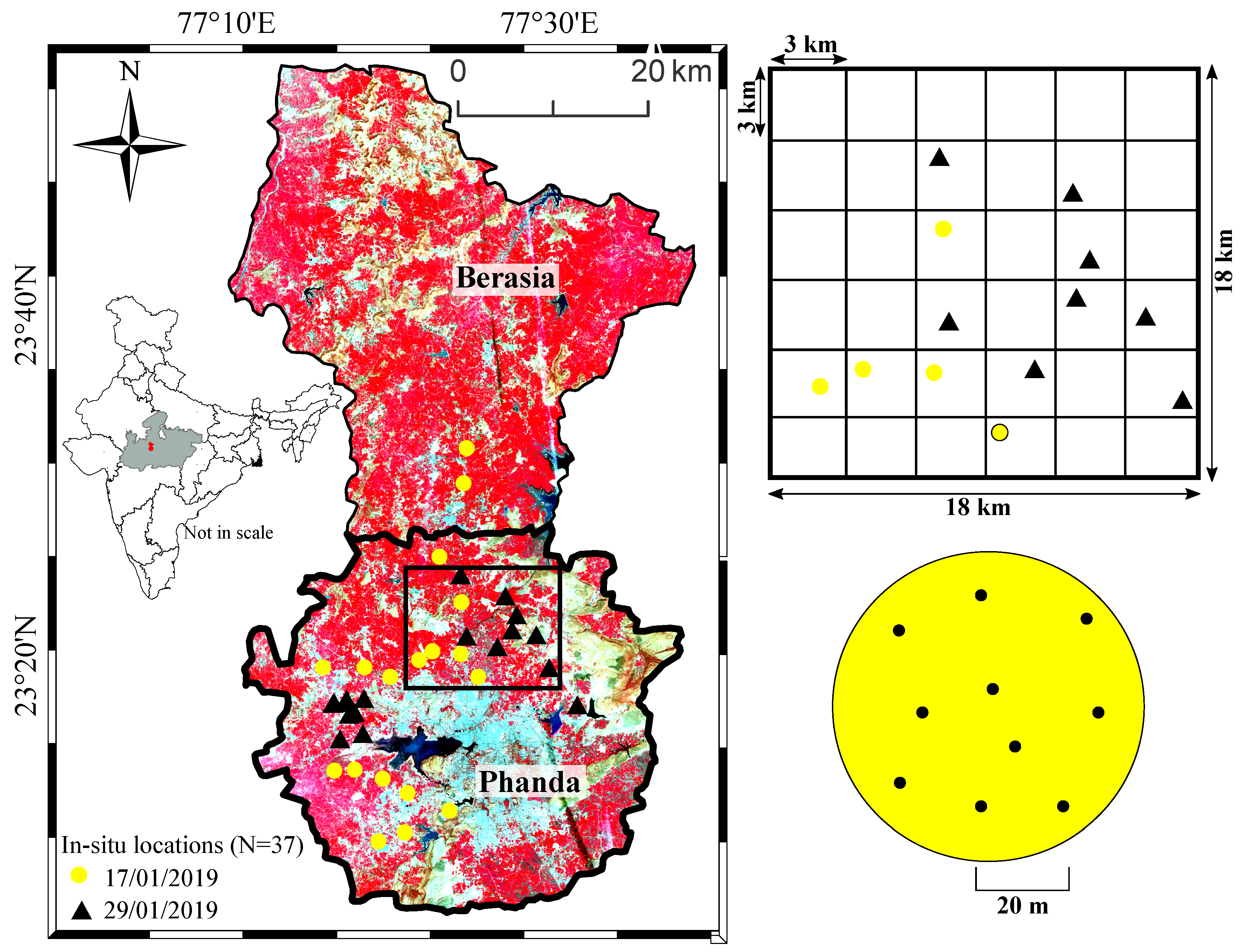
This study is conducted in Bhopal district of Madhya Pradesh in central India (
Figure 1). Bhopal is divided into two administrative blocks, Berasia in the north and Phanda in the south having a surface area of about 1424 km
and 1348 km
respectively (
Figure 1). Climatically, Bhopal lies in a semiarid zone and is typically covered by agriculture land (64.5%), barren land (7.3%), forest (13%), and water bodies (4.6%) [
44]. The average elevation in the study area varies between 450 and 550 m from the mean sea level with the gently undulated landscape. The average air temperature ranges between 6
C and 41
C. About 75% of the study area is covered by black cotton soil formed due to the weathering of basaltic rocks. The remaining 25% is covered with yellowish-red, mixed soils [
45,
46].
In this study, we have considered Phanda block as a test site to estimate soil moisture. About 44% of the area of Phanda is cultivable and used for agricultural purposes. The agricultural practice in the region largely depends on the Indian summer monsoon in June, July, August, and September (JJAS), where it receives about 92% of total rainfall.
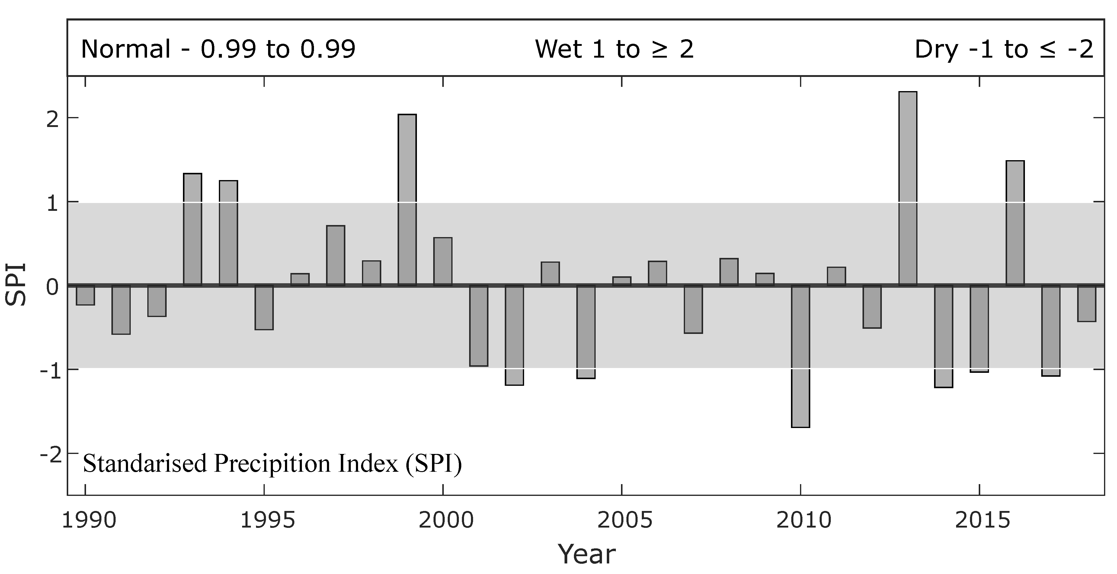
In recent years, the frequency of droughts in central India has increased, which has adversely impacted the agricultural productivity [
47]. To obtain the frequency of drought events in the study area, we have calculated Standardized Precipitation Index (SPI) for the monsoon period (JJAS) from 1990 to 2018 using gridded (
) rainfall data obtained from the Indian Meteorological Department [
48,
49]. SPI is used to characterise meteorological drought. For example, SPI values in a range between (−0.99 to 0.99) is considered normal, whereas SPI values less than −1 and greater than 1 are considered to be dry and wet period respectively [
50]. The SPI values of Phanda block (
Figure 2), clearly suggests that the frequency of drought events has increased in last two decades. In total, six drought events (2002, 2004, 2010, 2014, 2015, and 2017) have occurred between the years 2000 to 2018 (
Figure 2).
In this scenario, monitoring soil moisture at higher spatial and temporal resolution has become important in planning and management of agricultural productivity, water resources and ensuring food security. The landuse, geology, and soil types of the Phanda block makes it an ideal field site to study the soil moisture.
3. Material and Methods
3.1. Satellite Data
This study uses microwave and optical satellite images (
Table 1) to estimate soil moisture. We have downloaded publicly available Sentinel-1A images of two consecutive pass, i.e., 17 and 29 January 2019 from European Space Agency (
https://scihub.copernicus.eu/). Sentinel-1A, C-band SAR records the backscatter signals day and night, independent of the illumination and weather conditions. It acquires microwave images in four exclusive modes; Stripmap (SM), Interferometric Wide swath (IW), Extra Wide swath (EW), Wave (WV). It can capture images (in terms of polarization) using same set of transmitted pulses by using its antenna. Depending upon the acquisition mode, Sentinel-1 can acquires images in dual polarisation modes, Vertical–Vertical (VV) and Vertical–Horizontal (VH), or in single polarisation (HH or VV) at 10 m × 10 m cell size with a swath 250 km. At this swath, the incidence angle ranges between 29
to 46
for near and far range respectively. It has a temporal resolution of 12 days (in combination with Sentinel-1B the temporal resolution is 6 days). Microwave signals at C-band can penetrate up to 5 cm deep below the soil surface [
51,
52]. The Sentinel-1A level-1 data is categorised into two product types: Ground Range Detected (GRD) and Single Look Complex (SLC). Wide range of applications requires Sentinel-1A GRD product with standard corrections. After applying standard corrections, the Sentinel-1A GRD images will have square pixels (consisting of amplitude) with reduced speckle [
53,
54,
55,
56,
57]. We have also downloaded Landsat 8 images from the United States Geological Survey (
https://earthexplorer.usgs.gov/) pertaining to the date closest to the Sentinel-1A images. The Landsat 8 satellite mission carries a two-sensor payload, the Operational Land Imager (OLI) and the Thermal Infrared Sensor (TIRS). The OLI sensor consists of nine spectral bands (0.43–1.38
) and acquire images at 16 days revisit time with the spatial resolution 15 m for the panchromatic band (0.50–0.68
) and 30 m for the remaining bands [
58].
3.2. Field Measurement
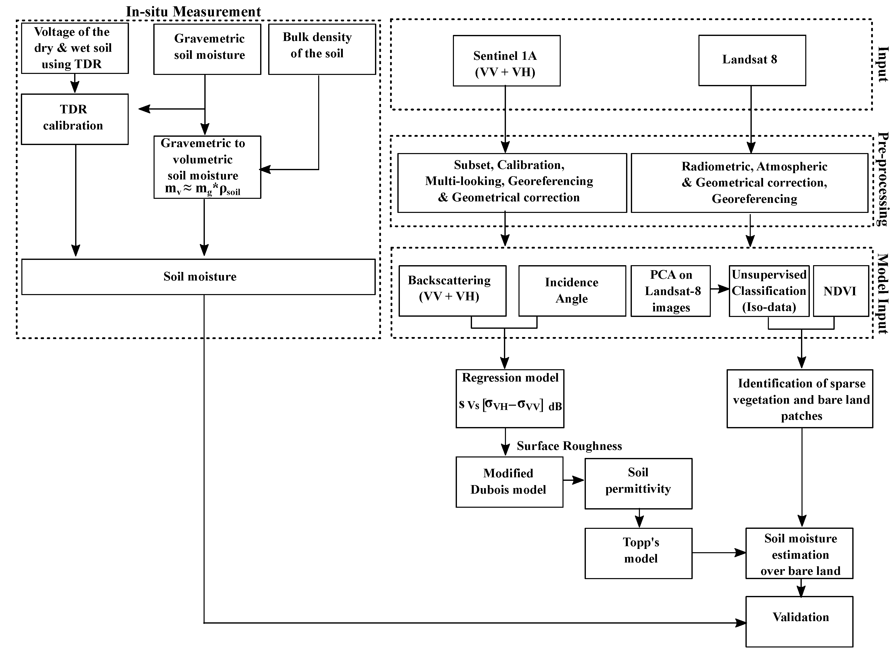
We have used ML3 theta probe sensor and gravimetric method to measure soil moisture in the field. Theta probe works on the principle of TDR, and it measures the bulk soil relative permittivity (
) at a frequency 100 MHz. This bulk relative permittivity is then converted into volumetric soil moisture by applying a soil specific calibration of TDR. We have calibrated the theta probe for three different dominant soil types of our study area. A detailed procedure of calibration is mentioned in the
Appendix A. To measure soil moisture, we have conducted a field campaign on 17 and 29 January 2019 in Bhopal, Madhya Pradesh. These dates coincide with the Sentinel-1A pass over Bhopal at 5:50 a.m. (IST). At the time of satellite passes, we have measured the soil moisture at 37 locations.
To conduct measurements, we overlay a square grid of
on our study area [
59]. We then randomly select few grids to measure the soil moisture. At the centre of each grid, we measured the soil moisture by inserting the metal rod of the theta probe at 5 cm below the ground surface and record the soil moisture value (
) in the data logger and acquired their locations using a Garmin-64S handheld GPS (
Figure 3a). We repeated this procedure at least in 8 to 10 different locations within the grid and finally averaged them to get soil moisture (
Figure 1). Simultaneously at each location, we have collected about 100 g of soil samples at 5 cm below the ground surface using tubular samplers (
Figure 3b). We used these samples to measure soil moisture by oven drying method (
Figure 3c). At each of the measurement location, we have also taken observations on land use, soil type, vegetation height and weather parameters (temperature, precipitation, etc.).
Table 2 reports the detailed characteristics and location of our sampling sites.
3.3. Data Processing
3.3.1. Soil Samples
We processed the soil samples in laboratory to measure their moisture content. We took about 100 g each of soil samples from a grid and placed them in a separate beaker (
Figure 3c). We placed the samples in an electric oven at 105
C for about 24 h [
60,
61]. Once the samples are completely dried, we weighed them. The difference between initial and dry weight provides the amount of moisture present in the soil samples. Eventually, we divide the weight of moisture content with the dry weight of soil samples. This quantity is the gravimetric soil moisture (
) and expressed in [kg/kg].
Since theta probe measures the volumetric soil moisture (
), we need to convert our laboratory measurement into comparable metric for any meaningful comparison. We multiply the gravimetric soil moisture (
) to the density ratio of soil (
) and water (
) to compute the volumetric soil moisture (
) in [
] according to;
3.3.2. Satellite Images
We have used Sentinel Application Platform (SNAP) v6.0 to process the Sentinel-1A images. The processing involves four major steps, radiometric calibration, multilook, speckle noise reduction using refined Lee filter, and terrain correction. Terrain or geometric calibration uses the Shuttle Radar Topography Mission (SRTM) digital elevation model of spatial resolution 30 m. The resulting image pixels contain the true backscatter () values on a linear scale. Finally, we convert the backscatter values into decibel scale () according to, . We have also processed Landsat-8 images to compute NDVI. It helps to measure the intensity of vegetation cover in terms of vegetation density and vegetation height. We take the ratio of the difference between band 5 (Near Infrared) and band 4 (Red) to the sum of band 5 and band 4 of Landsat-8 images. The NDVI is required to specify the validity range (NDVI ≤ 0.4) of modified Dubois model for soil moisture.
3.4. Soil Moisture Modelling
We have used the backscatter values of Sentinel-1A images and incidence angle in the modified Dubois model to calculate the relative soil permittivity. Finally, we used the relative permittivity in universal Topp’s model to compute volumetric soil moisture.
3.4.1. Radar Backscattering Model
Dubois et al. [
19] developed an empirical model to calculate the relative soil permittivity from quad polarised SAR images. Initially, this model was developed for L-, C- and X-band data obtained from scatterometer and later applied on airborne images as well. The model structure is developed on a strong physical reasoning; however, some of the unknown coefficients are obtained by fitting to the experimental data. The backscattering coefficient for HH and VV polarisation is given by Equations (
2) and (
3).
where
is the incidence angle,
is the relative soil permittivity,
s is the surface roughness (cm),
k =
is the wavenumber, and
is the SAR wavelength. These parameters can be grouped into two; sensor parameters (
and
) and target parameters (
and
s). In Equations (
2) and (
3), target parameters are unknown. These equations can be inverted to compute the relative soil permittivity and surface roughness parameters.
Dubois model is applicable for the SAR images acquired at incidence angle
between
to
and in the frequency range between 1.5–11 GHz. Further, this model is valid on the region having sparsely vegetation or barren land. The performance of the Dubois model is maximum where NDVI of the image pixels is less than 0.4 (Dubois NDVI criterion) or in the region on SAR images where the ratio of cross-polarised
is less than −11 dB [
19].
Dubois model was initially developed for quad polarised SAR images; it can not be directly applied to dual polarised data. In a study Rao et al. [
41] modified the Dubois model by incorporating in-situ measurements and field conditions and used the Equation (
2) to calculate the soil moisture from the SAR images acquired in HH polarisation.
To derive the unknown parameter (surface roughness) of Equation (
3), we obtain the parameter from regression model proposed by Srivastava et al. [
62]. Once surface roughness is known, Equation (
2) or (
3) can be solved to compute the other unknown, the relative soil permittivity. A flowchart in
Figure 4 illustrates the detailed methodology used for in-situ data acquisition, image processing and modelling to estimate soil moisture.
3.4.2. Estimation of Soil Moisture
To estimate soil moisture, we used Topp’s model [
63]. It takes the relative soil permittivity derived from Sentinel-1A image as an input to estimate volumetric soil moisture content according to Equation (
4). This model does not require a priori knowledge of soil properties (texture, grain size) and is proven to be a robust approach for the estimation of soil moisture [
64].
4. Results
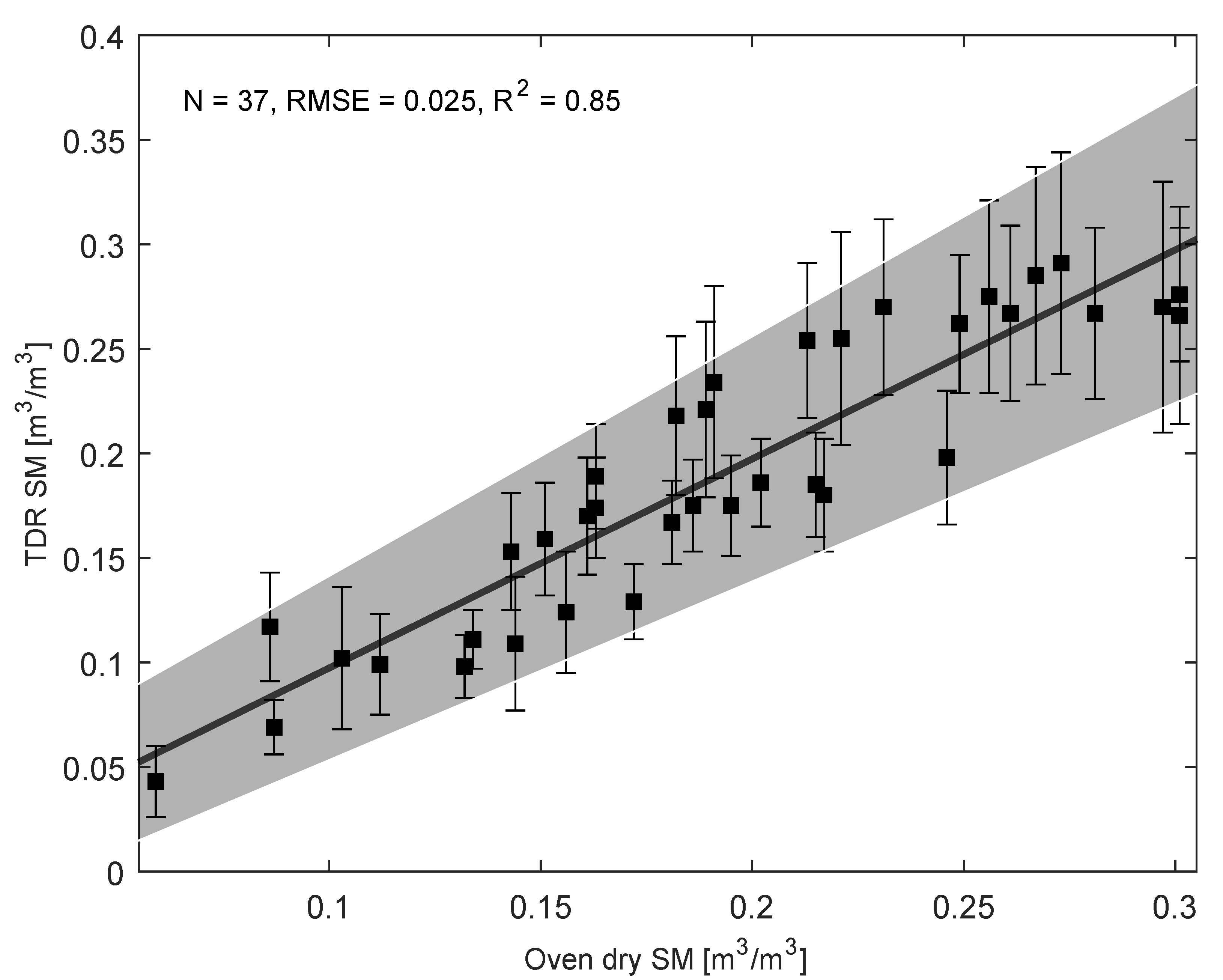
4.1. Performance of Calibrated Theta Probe
We compared the soil moisture measured from the theta probe and oven dry method. We observed no obvious difference, despite a mild scatter, all data points seem to gather around a single line (
Figure 5). This suggests a good agreement between (R
= 0.84 with RMSE = 0.025 m
/m
) both the methods, provided theta probe is correctly calibrated for the specific soil types in the study area. Hereafter we will use the measurements of theta probe for further analysis.
4.2. Soil Moisture from Sentinel-1A
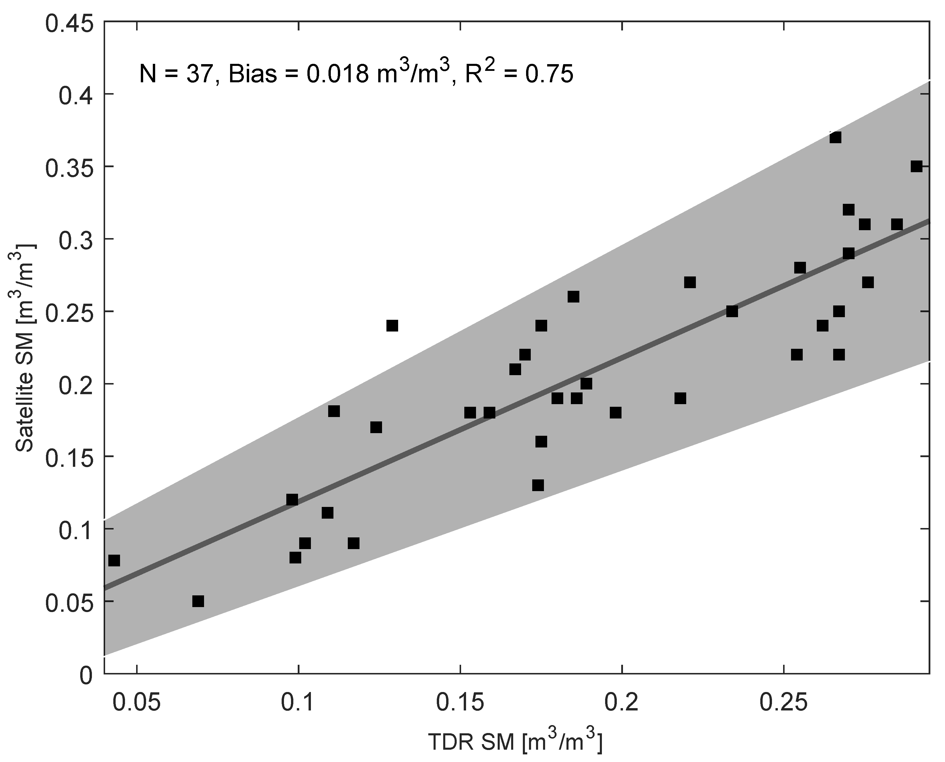
Once we calculated the soil moisture from Sentinel-1A images, we evaluated their accuracy with the in-situ measurement. We first identified the valid region for modified Dubois model using the Dubois NDVI criterion. For the locations where ground measurement is valid, we extracted the corresponding pixels from the modelled soil moisture maps. For both the dates, we observed a good agreement (R
) between the measured and modelled soil moisture (
Figure 6). However, at some locations, the difference between the modelled and measured values of soil moisture is comparatively large. This is probably due to the spatial scale mismatch, heterogeneous field conditions, measurement uncertainty, and model bias. When in-situ measurement is compared with the satellite derived soil moisture, a representative error arises due to the difference in the spatial scale of in-situ measurement and satellite observation. The spatial scale mismatch becomes more prominent when the land surface is heterogeneous. This limits the competency to compare the point measurement with the satellite [
65]. The error in the retrieval of soil moisture increases with the heterogeneity in land surface [
66]. Further, the measurement uncertainty is mainly due to the error associated with in-situ measurement. For example, error resulting from the conversion of dielectric constant to soil moisture in TDR, presence of organic matter in the soil, overestimation of drying condition in oven and difference in the sampling depth of the in-situ and satellite measurements [
67].
To reduce the measurement uncertainty, we have calibrated the TDR, removed the organic matter from soil the soil samples, and collected soil samples in the field according to the simulated penetration depth of the C-band SAR signal in the ground [
51]. Model error (or bias) is mainly due to the assumptions followed by its use.
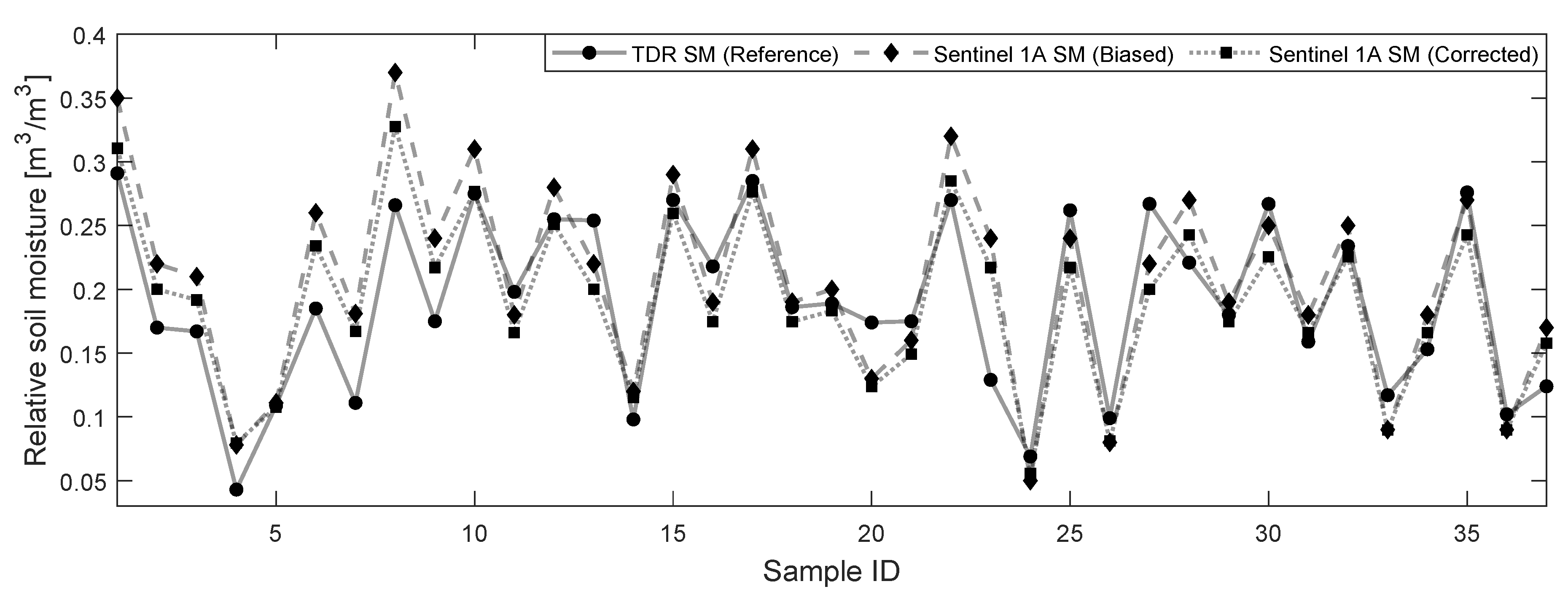
To overcome the systematic errors (instrument calibration and model error), we performed a bias correction by applying the CDF matching approach [
68]. This is one of the widely used statistical methods to minimise the bias in satellite-derived soil moisture [
69,
70,
71]. In principle, we adjusted the satellite-derived soil moisture according to the CDF of in-situ (TDR) soil moisture to minimise their difference (
Figure 7).
Applying the CDF correction on our data, biases in the soil moisture derived from Sentinel-1A has reduced from 0.02 m
/m
to 0.001 m
/m
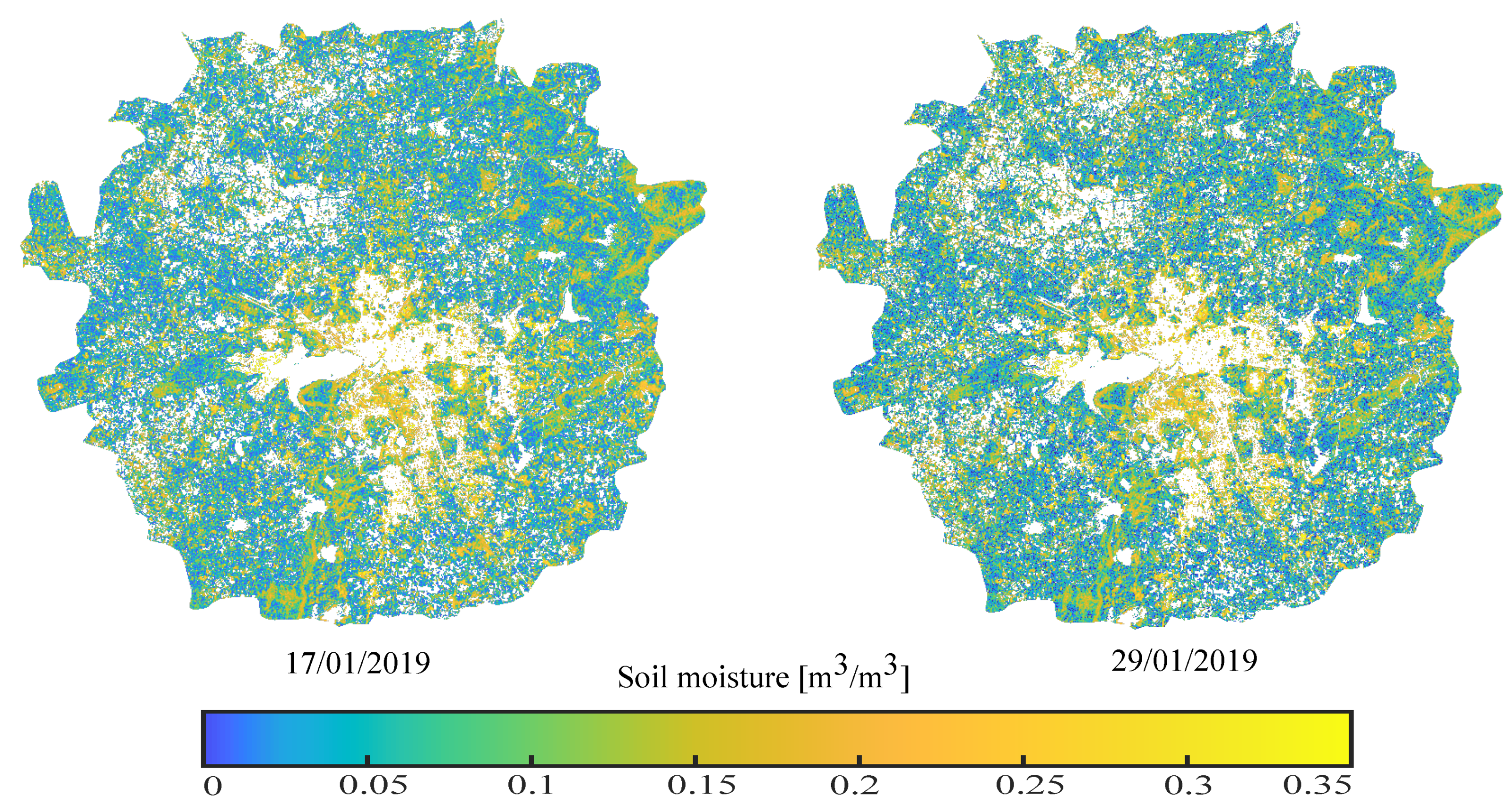
. Finally, we used the bias corrected values to generate soil moisture maps for 17 and 29 January 2019 (
Figure 8) of the study area.
5. Discussion
This study uses modified Dubois model to estimate soil moisture from dual polarised (VV and VH) Sentinel-1A images. Our result suggests that the model derived soil moisture accord well (R
= 0.75 and RMSE = 0.035 m
/m
) with the in-situ measurement (
Figure 6). This is consistent with the range of RMSE (0.03–0.04) m
/m
reported by other researchers [
72].
The modelled soil moisture is subject to bias due to various geometric, atmospheric and modelling errors. The magnitude of these uncertainties depends on various factors such as choice of a backscatter model, frequency of SAR images, ground condition and vegetation types. Several methods such as mean based (linear, local intensity and variance scaling) and the distribution-based (quantile and CDF matching) have been developed to correct the bias from the modelled soil moisture values [
68,
73,
74,
75,
76,
77].
We have used the CDF matching approach to minimize the bias from our modelled soil moisture. In doing so, we have adjusted the CDF of biased values according to the CDF of reference data. This has significantly reduced the bias from our modelled soil moisture.
Figure 9, shows the relative soil moisture values estimated from Sentinel-1A images before and after the CDF correction.
We observed, at some locations the modelled soil moisture is overestimated or underestimated with respect to the measured values. The underestimation is probably related to low backscattering coefficients from relatively smooth surfaces. Similarly, the overestimation of soil moisture could be associated with the high surface roughness resulting in high backscattering coefficients.
Though Sentinel-1A images provide a first-order estimation of soil moisture, modelling soil moisture from satellite images has substantial limitations and challenges. Most of the backscatter models used for the estimation of the relative soil permittivity from SAR backscatter are only valid for a specific range of soil moisture. For example, the modified Dubois model is valid for soil moisture in a range between 0 and 0.35 . Microwave SAR images with appropriate backscatter models can estimate soil moisture only upto a few cms below the soil surface. In our case, we have estimated the soil moisture from the top about 5 cm below the ground surface. Further, many of the existing backscatter models are applicable for specific landuse and landcover classes. For example, Oh and water cloud models are applicable for barren and vegetated lands, respectively. The modified Dubois model can be applied on both barren and sparsely vegetated (NDVI ≤ 0.4) land. In summary, modified Dubois model performs well over the semi-arid region on agriculture and barren land. The performance is further improved when the bias correction method is used.
Moreover, estimation of soil moisture from C-band SAR is sensitive to various parameters such as; the incidence angle, polarisation, vegetation height and vegetation indices, i.e., Leaf Area Index (LAI). Ulaby [
13] observed that in a typical agricultural field (LAI > 0.5), the effect of vegetation is more prominent in the radar backscatter compared to other target properties.
As a consequence, when the vegetation effect starts dominating, it complicates the soil moisture retrieval. The backscatter values results from the combined signature of vegetation and underlying soil water [
78]. In such condition we can not ignore the attenuation due to vegetation. To minimise the effect of vegetation, scattering model such as the WCM can be implemented [
79,
80,
81,
82,
83].
6. Conclusions
We have shown that the modified Dubois model provides a good estimate (R = 0.75) of soil moisture in a region of heterogeneous land cover. The modelled soil moisture is subject to error due to the model (systematic) and sampling (random) errors. We have shown that the systematic error (also called systematic bias) can be largely minimised by the CDF matching technique. Whereas random errors can be reduced by increasing the number of sample size.
We found that the VV polarisation of Sentinel-1A is suitable for soil moisture monitoring. This is mainly because the VV polarisation is more sensitive to the soil contribution. In contrast, VH polarisation is more sensitive to the volume scattering, and it describes the vegetation contribution more effectively. Since our model is only for VV or HH, we have used the VV polarisation based on the polarisation of the Sentinel-1A data.
Further, the potential of VV and HH polarisation of Sentinel-1A may be evaluated, especially for the models (i.e., WCM) that can estimate soil moisture in diverse vegetation condition. Finally, our first-order analysis calls for a more detailed study on soil moisture modelling from Sentinel-1A images in diverse soil, landuse and landcover conditions.
This study is a step towards monitoring the surface soil moisture at higher spatial and temporal resolution from remote sensing data. Our methodology can be used to predict and monitor meteorological droughts, agricultural productivity and managing water resources in the region.
Author Contributions
Conceptualization, A.S. and K.G.; methodology, A.S., G.K.M. and K.G.; software, A.S. and K.G.; validation, G.K.M., A.S. and K.G.; formal analysis, A.S. and G.K.M.; investigation, K.G. and A.S.; resources, K.G. and S.K.; data curation, G.K.M., A.S. and K.G.; writing—original draft preparation, A.S. and K.G.; writing—review and editing, K.G. and A.S.; visualization, K.G. and S.K.; supervision and project administration, K.G.; funding acquisition, K.G. and S.K. All authors have read and agreed to the published version of the manuscript.
Funding
This research was funded by the Space Applications Centre (SAC-ISRO) under NASA-ISRO Synthetic Aperture Radar (NISAR) mission through grant Hyd-01.
Acknowledgments
We would like to acknowledge IISER Bhopal for providing institutional support. Abhilash Singh PhD is supported by the Department of Science and Technology (DST), Government of India through DST-INSPIRE fellowship. We gratefully acknowledge Prof. S.K. Tandon for fruitful suggestions. We thanks to the editor and all the three anonymous reviewers for providing helpful comments and suggestions.
Conflicts of Interest
The authors declare no conflict of interest.
Appendix A
Theta probe (ML3 sensor) requires an intensive soil specific and a sensor specific calibration before being used for data acquisition in the field. The soil specific calibration explores a functional relationship between the relative soil permittivity and soil moisture. In contrast, the sensor specific calibration explores the functional relationship between the relative soil permittivity and ML3 output (volts). Both the soil and sensor specific calibration equations are combined to finally convert the sensor output directly into soil moisture. The soil specific calibration allows to find the two constants (
,
) of Equation (
A1).
For sensor calibration, ML3 sensor measures the bulk relative soil permittivity using the empirical relation given by Equation (
A2);
where,
V is the voltage in Volt. Combining soil and sensor specific calibration equation reads (Equation (
A3));
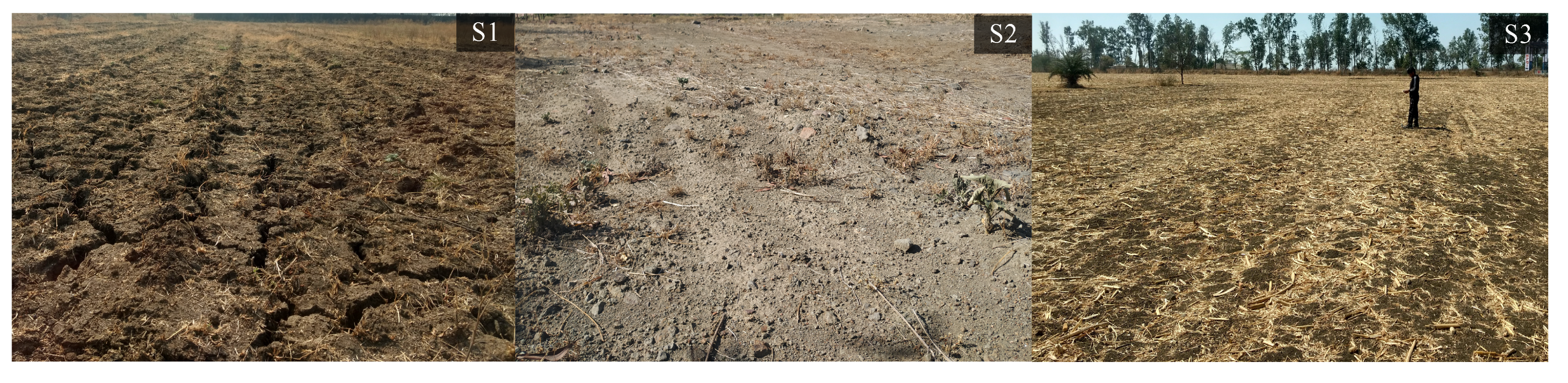
Before the field campaign, we have calibrated the theta probe at three different locations in the study area (
Figure A1).
Figure A1.
Soil samples used from three different fields for the calibration of MLT-3 theta probe. Samples from S1 and S3 corresponds to agricultural lands composed of black cotton soil and rich in organic matters. S2 consists of black soil with granules rubble (about 20–25%) formed due to the subsequent weathering of Deccan basalt.
The corresponding values of the calibration constant is given
Table A1.
Table A1.
Field derived calibration constants for MLT-3 theta probe.
Table A1.
Field derived calibration constants for MLT-3 theta probe.
| Measuring Unit | Site 1 (S1) | Site 2 (S2) | Site 3 (S3) |
|---|
| (cm) | 563 | 563 | 563 |
| (gm) | 491 | 505 | 504 |
| (mV) | 342 | 333 | 350 |
| (gm) | 410 | 415 | 421 |
| (mV) | 101 | 72 | 90 |
| 1.6 | 1.5 | 1.6 |
| 7.1 | 7.4 | 7.6 |
To calculate
and
, we have measured two voltage from Equation (
A2).
and
correspond to the dry and wet samples respectively. We have also measured wet weight (
) and dry weight (
) of the samples.
Calculation of : For dry soil (i.e.,
=0), Equation (
A1), is reduced to
=
. Substituting the value of
in Equation (
A2), we have calculated the value of
. Eventually we calculated
according to;
Calculation of : For wet soil, we calculated the soil moisture as;
where,
is the volume occupied by the sample in the beaker. By substituting the value of
in Equation (
A2), we have calculated the values of
. Finally
is calculated according to;
References
- Kite, G.; Pietroniro, A. Remote sensing applications in hydrological modelling. Hydrol. Sci. J. 1996, 41, 563–591. [Google Scholar] [CrossRef]
- Jackson, T.J. Measuring surface soil moisture using passive microwave remote sensing. Hydrol. Process. 1993, 7, 139–152. [Google Scholar] [CrossRef]
- Entekhabi, D. Retrieval of Soil Moisture Profile by Combined Remote Sensing and Modeling. 1993. Available online: https://trs.jpl.nasa.gov/handle/2014/34543 (accessed on 11 May 2020).
- Jackson, T.; Hawley, M.; O’neill, P. Preplanting soil moisture using passive microwave sensor. JAWRA J. Am. Water Resour. Assoc. 1987, 23, 11–19. [Google Scholar] [CrossRef]
- Martin, M.E.; Aber, J.D. High spectral resolution remote sensing of forest canopy lignin, nitrogen, and ecosystem processes. Ecol. Appl. 1997, 7, 431–443. [Google Scholar] [CrossRef]
- Sivapalan, M.; Takeuchi, K.; Franks, S.; Gupta, V.; Karambiri, H.; Lakshmi, V.; Liang, X.; McDonnell, J.; Mendiondo, E.; O’connell, P. IAHS Decade on Predictions in Ungauged Basins (PUB), 2003–2012: Shaping an exciting future for the hydrological sciences. Hydrol. Sci. J. 2003, 48, 857–880. [Google Scholar] [CrossRef] [Green Version]
- Field, C.B.; Randerson, J.T.; Malmström, C.M. Global net primary production: Combining ecology and remote sensing. Remote Sens. Environ. 1995, 51, 74–88. [Google Scholar] [CrossRef] [Green Version]
- Seneviratne, S.I.; Corti, T.; Davin, E.L.; Hirschi, M.; Jaeger, E.B.; Lehner, I.; Orlowsky, B.; Teuling, A.J. Investigating soil moisture–climate interactions in a changing climate: A review. Earth-Sci. Rev. 2010, 99, 125–161. [Google Scholar] [CrossRef]
- Kerr, J.T.; Ostrovsky, M. From space to species: Ecological applications for remote sensing. Trends Ecol. Evol. 2003, 18, 299–305. [Google Scholar] [CrossRef]
- Mulla, D.J. Twenty five years of remote sensing in precision agriculture: Key advances and remaining knowledge gaps. Biosyst. Eng. 2013, 114, 358–371. [Google Scholar] [CrossRef]
- Walker, J.P. Estimating Soil Moisture Profile Dynamics from Near-Surface Soil Moisture Measurements and Standard Meteorological Data. Ph.D. Thesis, University of Newcastle, Callaghan, Australia, 1999. [Google Scholar]
- Narvekar, P.S.; Entekhabi, D.; Kim, S.; Njoku, E.G. Soil Moisture Retrieval Using L-Band Radar Observations. IEEE Trans. Geosci. Remote Sens. 2015, 53, 3492–3506. [Google Scholar] [CrossRef]
- Ulaby, F.T. Microwave remote sensing active and passive. In Rader Remote Sensing and Surface Scattering and Emission Theory; NASA Technical Report; Kansas University: Lawrence, KS, USA, 1982; pp. 848–902. [Google Scholar]
- Altese, E.; Bolognani, O.; Mancini, M.; Troch, P.A. Retrieving soil moisture over bare soil from ERS 1 synthetic aperture radar data: Sensitivity analysis based on a theoretical surface scattering model and field data. Water Resour. Res. 1996, 32, 653–661. [Google Scholar] [CrossRef]
- Verhoest, N.E.; Lievens, H.; Wagner, W.; Álvarez-Mozos, J.; Moran, M.S.; Mattia, F. On the soil roughness parameterization problem in soil moisture retrieval of bare surfaces from synthetic aperture radar. Sensors 2008, 8, 4213–4248. [Google Scholar] [CrossRef] [Green Version]
- Barrett, B.W.; Dwyer, E.; Whelan, P. Soil moisture retrieval from active spaceborne microwave observations: An evaluation of current techniques. Remote Sens. 2009, 1, 210–242. [Google Scholar] [CrossRef] [Green Version]
- Oh, Y.; Sarabandi, K.; Ulaby, F.T. An empirical model and an inversion technique for radar scattering from bare soil surfaces. IEEE Trans. Geosci. Remote Sens. 1992, 30, 370–381. [Google Scholar] [CrossRef]
- Oh, Y.; Sarabandi, K.; Ulaby, F.T. An inversion algorithm for retrieving soil moisture and surface roughness from polarimetric radar observation. In Proceedings of the IEEE International Geoscience and Remote Sensing Symposium, Pasadena, CA, USA, 8–12 August 1994; Volume 3, pp. 1582–1584. [Google Scholar]
- Dubois, P.C.; Van Zyl, J.; Engman, T. Measuring soil moisture with imaging radars. IEEE Trans. Geosci. Remote Sens. 1995, 33, 915–926. [Google Scholar] [CrossRef] [Green Version]
- Oh, Y.; Sarabandi, K.; Ulaby, F.T. Semi-empirical model of the ensemble-averaged differential Mueller matrix for microwave backscattering from bare soil surfaces. IEEE Trans. Geosci. Remote Sens. 2002, 40, 1348–1355. [Google Scholar] [CrossRef] [Green Version]
- Oh, Y. Quantitative retrieval of soil moisture content and surface roughness from multipolarized radar observations of bare soil surfaces. IEEE Trans. Geosci. Remote Sens. 2004, 42, 596–601. [Google Scholar] [CrossRef]
- Attema, E.; Ulaby, F.T. Vegetation modeled as a water cloud. Radio Sci. 1978, 13, 357–364. [Google Scholar] [CrossRef]
- Fung, A.K.; Li, Z.; Chen, K.S. Backscattering from a randomly rough dielectric surface. IEEE Trans. Geosci. Remote Sens. 1992, 30, 356–369. [Google Scholar] [CrossRef]
- Fung, A.K.; Cheng, K.S. Microwave Scattering and Emission Models and Their Applications; Artech House Inc.: Boston, MA, USA, 1994. [Google Scholar]
- Baghdadi, N.; Cresson, R.; El Hajj, M.; Ludwig, R.; La Jeunesse, I. Soil parameters estimation over bare agriculture areas from C-band polarimetric SAR data using neural networks. Hydrol. Earth Syst. Sci. Discuss. 2012, 9, 2897–2933. [Google Scholar] [CrossRef] [Green Version]
- El Hajj, M.; Baghdadi, N.; Zribi, M.; Belaud, G.; Cheviron, B.; Courault, D.; Charron, F. Soil moisture retrieval over irrigated grassland using X-band SAR data. Remote Sens. Environ. 2016, 176, 202–218. [Google Scholar] [CrossRef] [Green Version]
- Dabrowska-Zielinska, K.; Musial, J.; Malinska, A.; Budzynska, M.; Gurdak, R.; Kiryla, W.; Bartold, M.; Grzybowski, P. Soil moisture in the Biebrza Wetlands retrieved from Sentinel-1 imagery. Remote Sens. 2018, 10, 1979. [Google Scholar] [CrossRef] [Green Version]
- Wagner, W.; Pathe, C.; Doubkova, M.; Sabel, D.; Bartsch, A.; Hasenauer, S.; Blöschl, G.; Scipal, K.; Martínez-Fernández, J.; Löw, A. Temporal stability of soil moisture and radar backscatter observed by the Advanced Synthetic Aperture Radar (ASAR). Sensors 2008, 8, 1174–1197. [Google Scholar] [CrossRef] [PubMed] [Green Version]
- Zribi, M.; Muddu, S.; Bousbih, S.; Al Bitar, A.; Tomer, S.K.; Baghdadi, N.; Bandyopadhyay, S. Analysis of L-band SAR data for soil moisture estimations over agricultural areas in the tropics. Remote Sens. 2019, 11, 1122. [Google Scholar] [CrossRef] [Green Version]
- Yang, L.; Feng, X.; Liu, F.; Liu, J.; Sun, X. Potential of soil moisture estimation using C-band polarimetric SAR data in arid regions. Int. J. Remote Sens. 2019, 40, 2138–2150. [Google Scholar] [CrossRef]
- El Hajj, M.; Baghdadi, N.; Zribi, M.; Bazzi, H. Synergic use of Sentinel-1 and Sentinel-2 images for operational soil moisture mapping at high spatial resolution over agricultural areas. Remote Sens. 2017, 9, 1292. [Google Scholar] [CrossRef] [Green Version]
- Bousbih, S.; Zribi, M.; El Hajj, M.; Baghdadi, N.; Lili-Chabaane, Z.; Gao, Q.; Fanise, P. Soil moisture and irrigation mapping in A semi-arid region, based on the synergetic use of Sentinel-1 and Sentinel-2 data. Remote Sens. 2018, 10, 1953. [Google Scholar] [CrossRef] [Green Version]
- Qiu, J.; Crow, W.T.; Wagner, W.; Zhao, T. Effect of vegetation index choice on soil moisture retrievals via the synergistic use of synthetic aperture radar and optical remote sensing. Int. J. Appl. Earth Obs. Geoinf. 2019, 80, 47–57. [Google Scholar] [CrossRef]
- Hachani, A.; Ouessar, M.; Paloscia, S.; Santi, E.; Pettinato, S. Soil moisture retrieval from Sentinel-1 acquisitions in an arid environment in Tunisia: Application of Artificial Neural Networks techniques. Int. J. Remote Sens. 2019, 40, 9159–9180. [Google Scholar] [CrossRef]
- Ezzahar, J.; Ouaadi, N.; Zribi, M.; Elfarkh, J.; Aouade, G.; Khabba, S.; Er-Raki, S.; Chehbouni, A.; Jarlan, L. Evaluation of Backscattering Models and Support Vector Machine for the Retrieval of Bare Soil Moisture from Sentinel-1 Data. Remote Sens. 2020, 12, 72. [Google Scholar] [CrossRef] [Green Version]
- Hosseini, M.; McNairn, H. Using multi-polarization C-and L-band synthetic aperture radar to estimate biomass and soil moisture of wheat fields. Int. J. Appl. Earth Obs. Geoinf. 2017, 58, 50–64. [Google Scholar] [CrossRef]
- Dave, R.; Kumar, G.; Kr. Pandey, D.; Khan, A.; Bhattacharya, B. Evaluation of modified Dubois model for estimating surface soil moisture using dual polarization RISAT-1 C-band SAR data. Geocarto Int. 2019, 1–11. [Google Scholar] [CrossRef]
- Alexakis, D.D.; Mexis, F.D.K.; Vozinaki, A.E.K.; Daliakopoulos, I.N.; Tsanis, I.K. Soil moisture content estimation based on Sentinel-1 and auxiliary earth observation products. A hydrological approach. Sensors 2017, 17, 1455. [Google Scholar] [CrossRef] [Green Version]
- Wagner, W.; Sabel, D.; Doubkova, M.; Bartsch, A.; Pathe, C. The potential of Sentinel-1 for monitoring soil moisture with a high spatial resolution at global scale. In Proceedings of the Earth Observation and Water Cycle Science, Frascati, Italy, 18–20 November 2009. [Google Scholar]
- Bauer-Marschallinger, B.; Freeman, V.; Cao, S.; Paulik, C.; Schaufler, S.; Stachl, T.; Modanesi, S.; Massari, C.; Ciabatta, L.; Brocca, L.; et al. Toward global soil moisture monitoring with Sentinel-1: Harnessing assets and overcoming obstacles. IEEE Trans. Geosci. Remote Sens. 2018, 57, 520–539. [Google Scholar] [CrossRef]
- Rao, S.S.; Das, S.; Nagaraju, M.; Venugopal, M.; Rajankar, P.; Laghate, P.; Reddy, M.S.; Joshi, A.; Sharma, J. Modified Dubois model for estimating soil moisture with dual polarized SAR data. J. Indian Soc. Remote Sens. 2013, 41, 865–872. [Google Scholar]
- Thanabalan, P.; Vidhya, R. A synergistic approach for soil moisture estimation using modified Dubois model with dual-polarized SAR and optical satellite data. Proc. SPIE 2016, 9877. [Google Scholar] [CrossRef]
- Mirsoleimani, H.R.; Sahebi, M.R.; Baghdadi, N.; El Hajj, M. Bare soil surface moisture retrieval from sentinel-1 SAR data based on the calibrated IEM and Dubois models using neural networks. Sensors 2019, 19, 3209. [Google Scholar] [CrossRef] [Green Version]
- NRSC. District and Category Wise Distribution of Land Use and Land Cover in Madhya Pradesh (2015-16). Available online: https://bhuvan-app1.nrsc.gov.in/2dresources/thematic/LULC503/MAP/MP.pdf (accessed on 25 May 2020).
- Ministry of Water Resources, Central Ground Water Board, North Central Region, Bhopal. District Ground Water Information Booklet. Available online: http://cgwb.gov.in/District_Profile/MP/Bhopal.pdf (accessed on 25 May 2020).
- Central Ground Water Board, Ministry of Water Resources, River Development and Ganga Rejuvenation, Government of India. Aquifer Mapping Report Phanda Block, Bhopal District, Madhya Pradesh. Available online: http://cgwb.gov.in/AQM/NAQUIM_REPORT/MP/PhandaBlockBhopal.pdf (accessed on 25 May 2020).
- Mishra, V.; Shah, R.; Garg, A. Climate Change in Madhya Pradesh: Indicators, Impacts and Adaptation; Indian Institute of Management Ahmadabad: Ahmedabad, India, 2016. [Google Scholar]
- Pai, D.; Sridhar, L.; Rajeevan, M.; Sreejith, O.; Satbhai, N.; Mukhopadhyay, B. Development of a new high spatial resolution (0.25 × 0.25) long period (1901–2010) daily gridded rainfall data set over India and its comparison with existing data sets over the region. Mausam 2014, 65, 1–18. [Google Scholar]
- Indian Meteorological Department. Rainfall Data. Available online: http://www.imdpune.gov.in/Clim_Pred_LRF_New/Grided_Data_Download.html (accessed on 25 May 2020).
- Hayes, M.J.; Svoboda, M.D.; Wiihite, D.A.; Vanyarkho, O.V. Monitoring the 1996 drought using the standardized precipitation index. Bull. Am. Meteorol. Soc. 1999, 80, 429–438. [Google Scholar] [CrossRef] [Green Version]
- Singh, A.; Meena, G.K.; Kumar, S.; Gaurav, K. Analysis of the effect of incidence angle and moisture content on the penetration depth of L-and S-band SAR signals into the ground surface. ISPRS Ann. Photogramm. Remote Sens. Spat. Inf. Sci. 2018, 4, 197–202. [Google Scholar] [CrossRef] [Green Version]
- Singh, A.; Meena, G.K.; Kumar, S.; Gaurav, K. Evaluation of the Penetration Depth of L-and S-Band (NISAR mission) Microwave SAR Signals into Ground. In Proceedings of the 2019 URSI Asia-Pacific Radio Science Conference (AP-RASC), New Delhi, India, 9–15 March 2019. [Google Scholar]
- Potin, P.; Rosich, B.; Grimont, P.; Miranda, N.; Shurmer, I.; O’Connell, A.; Torres, R.; Krassenburg, M. Sentinel-1 mission status. In Proceedings of the EUSAR 2016: 11th European Conference on Synthetic Aperture Radar, Hamburg, Germany, 6–9 June 2016; pp. 1–6. [Google Scholar]
- Filipponi, F. Sentinel-1 GRD Preprocessing Workflow. 3rd International Electronic Conference on Remote Sensing. Proceedings 2019, 18, 11. [Google Scholar] [CrossRef] [Green Version]
- Frison, P.L.; Fruneau, B.; Kmiha, S.; Soudani, K.; Dufrêne, E.; Le Toan, T.; Koleck, T.; Villard, L.; Mougin, E.; Rudant, J.P. Potential of Sentinel-1 data for monitoring temperate mixed forest phenology. Remote Sens. 2018, 10, 2049. [Google Scholar] [CrossRef] [Green Version]
- Gao, Q.; Zribi, M.; Escorihuela, M.J.; Baghdadi, N. Synergetic use of Sentinel-1 and Sentinel-2 data for soil moisture mapping at 100 m resolution. Sensors 2017, 17, 1966. [Google Scholar] [CrossRef] [Green Version]
- Martinis, S.; Plank, S.; Ćwik, K. The use of Sentinel-1 time-series data to improve flood monitoring in arid areas. Remote Sens. 2018, 10, 583. [Google Scholar] [CrossRef] [Green Version]
- Roy, D.P.; Wulder, M.A.; Loveland, T.R.; Woodcock, C.; Allen, R.G.; Anderson, M.C.; Helder, D.; Irons, J.R.; Johnson, D.M.; Kennedy, R.; et al. Landsat-8: Science and product vision for terrestrial global change research. Remote Sens. Environ. 2014, 145, 154–172. [Google Scholar] [CrossRef] [Green Version]
- Guo, M. Soil sampling and methods of analysis. J. Environ. Qual. 2009, 38, 375. [Google Scholar] [CrossRef]
- Gardner, C.M.; Robinson, D.A.; Blyth, K.; Cooper, J.D. Soil water content. In Soil and Environmental Analysis: Physical Methods; Smith, K.A., Mullins, C.E., Eds.; Marcel Dekker: New York, NY, USA, 2001; pp. 1–64. [Google Scholar]
- Reynolds, S. The gravimetric method of soil moisture determination Part I. A study of equipment, and methodological problems. J. Hydrol. 1970, 11, 258–273. [Google Scholar] [CrossRef]
- Srivastava, H.; Patel, P.; Navalgund, R.; Sharma, Y. Retrieval of surface roughness using multi-polarized Envisat-1 ASAR data. Geocarto Int. 2008, 23, 67–77. [Google Scholar] [CrossRef]
- Topp, G.C.; Davis, J.; Annan, A.P. Electromagnetic determination of soil water content: Measurements in coaxial transmission lines. Water Resour. Res. 1980, 16, 574–582. [Google Scholar] [CrossRef] [Green Version]
- Song, K.; Zhou, X.; Fan, Y. Empirically adopted IEM for retrieval of soil moisture from radar backscattering coefficients. IEEE Trans. Geosci. Remote Sens. 2009, 47, 1662–1672. [Google Scholar] [CrossRef]
- Talone, M.; Camps, A.; Monerris, A.; Vall-llossera, M.; Ferrazzoli, P.; Piles, M. Surface topography and mixed-pixel effects on the simulated L-band brightness temperatures. IEEE Trans. Geosci. Remote Sens. 2007, 45, 1996–2003. [Google Scholar] [CrossRef]
- Zhang, T.; Zhang, L.; Jiang, L.; Zhao, S.; Zhao, T.; Li, Y. Effects of spatial distribution of soil parameters on soil moisture retrieval from passive microwave remote sensing. Sci. China Earth Sci. 2012, 55, 1313–1322. [Google Scholar] [CrossRef]
- Lee, J.H.; Zhao, C.; Kerr, Y. Stochastic bias correction and uncertainty estimation of satellite-retrieved soil moisture products. Remote Sens. 2017, 9, 847. [Google Scholar] [CrossRef] [Green Version]
- Michelangeli, P.A.; Vrac, M.; Loukos, H. Probabilistic downscaling approaches: Application to wind cumulative distribution functions. Geophys. Res. Lett. 2009, 36, 1–6. [Google Scholar] [CrossRef]
- Reichle, R.H. Data assimilation methods in the Earth sciences. Adv. Water Resour. 2008, 31, 1411–1418. [Google Scholar] [CrossRef]
- Reichle, R.H.; Koster, R.D. Bias reduction in short records of satellite soil moisture. Geophys. Res. Lett. 2004, 31, 1–4. [Google Scholar] [CrossRef] [Green Version]
- Draper, C.; Mahfouf, J.F.; Walker, J.P. An EKF assimilation of AMSR-E soil moisture into the ISBA land surface scheme. J. Geophys. Res. Atmos. 2009, 114, 1–13. [Google Scholar] [CrossRef] [Green Version]
- Hosseini, R.; Newlands, N.K.; Dean, C.B.; Takemura, A. Statistical modeling of soil moisture, integrating satellite remote-sensing (SAR) and ground-based data. Remote Sens. 2015, 7, 2752–2780. [Google Scholar] [CrossRef] [Green Version]
- Kumar, S.; Peters-Lidard, C.; Santanello, J.; Reichle, R.; Draper, C.; Koster, R.; Nearing, G.; Jasinski, M. Evaluating the utility of satellite soil moisture retrievals over irrigated areas and the ability of land data assimilation methods to correct for unmodeled processes. Hydrol. Earth Syst. Sci. 2015, 19, 4463–4478. [Google Scholar] [CrossRef] [Green Version]
- Leander, R.; Buishand, T.A. Resampling of regional climate model output for the simulation of extreme river flows. J. Hydrol. 2007, 332, 487–496. [Google Scholar] [CrossRef]
- Schmidli, J.; Frei, C.; Vidale, P.L. Downscaling from GCM precipitation: A benchmark for dynamical and statistical downscaling methods. Int. J. Climatol. 2006, 26, 679–689. [Google Scholar] [CrossRef]
- Lenderink, G.; Buishand, A.; Deursen, W.V. Estimates of future discharges of the river Rhine using two scenario methodologies: Direct versus delta approach. Hydrol. Earth Syst. Sci. 2007, 11, 1145–1159. [Google Scholar] [CrossRef]
- Panofsky, H.A.; Brier, G.W. Some Applications of Statistics to Meteorology; Pennsylvania State University: Pennsylvania, PA, USA, 1958. [Google Scholar]
- He, B.; Xing, M.; Bai, X. A synergistic methodology for soil moisture estimation in an alpine prairie using radar and optical satellite data. Remote Sens. 2014, 6, 10966–10985. [Google Scholar] [CrossRef] [Green Version]
- Bindlish, R.; Barros, A.P. Parameterization of vegetation backscatter in radar-based, soil moisture estimation. Remote Sens. Environ. 2001, 76, 130–137. [Google Scholar] [CrossRef]
- Gherboudj, I.; Magagi, R.; Berg, A.A.; Toth, B. Soil moisture retrieval over agricultural fields from multi-polarized and multi-angular RADARSAT-2 SAR data. Remote Sens. Environ. 2011, 115, 33–43. [Google Scholar] [CrossRef]
- Du, J.; Shi, J.; Sun, R. The development of HJ SAR soil moisture retrieval algorithm. Int. J. Remote Sens. 2010, 31, 3691–3705. [Google Scholar] [CrossRef]
- Lievens, H.; Verhoest, N.E. On the retrieval of soil moisture in wheat fields from L-band SAR based on water cloud modeling, the IEM, and effective roughness parameters. IEEE Geosci. Remote Sens. Lett. 2011, 8, 740–744. [Google Scholar] [CrossRef]
- De Roo, R.D.; Du, Y.; Ulaby, F.T.; Dobson, M.C. A semi-empirical backscattering model at L-band and C-band for a soybean canopy with soil moisture inversion. IEEE Trans. Geosci. Remote Sens. 2001, 39, 864–872. [Google Scholar] [CrossRef]
© 2020 by the authors. Licensee MDPI, Basel, Switzerland. This article is an open access article distributed under the terms and conditions of the Creative Commons Attribution (CC BY) license (http://creativecommons.org/licenses/by/4.0/).


