Can We Measure a COVID-19-Related Slowdown in Atmospheric CO2 Growth? Sensitivity of Total Carbon Column Observations

Karlsruhe Institute of Technology, IMK-IFU, 82467 Garmisch-Partenkirchen, Germany
*
Author to whom correspondence should be addressed.
Remote Sens. 2020, 12(15), 2387; https://0-doi-org.brum.beds.ac.uk/10.3390/rs12152387
Submission received: 17 June 2020
/
Revised: 17 July 2020
/
Accepted: 21 July 2020
/
Published: 24 July 2020
(This article belongs to the Special Issue Remote Sensing of Greenhouse Gases and Air Pollution)
Abstract
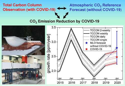
:The COVID-19 pandemic is causing projected annual CO2 emission reductions up to −8% for 2020. This approximately matches the reductions required year on year to fulfill the Paris agreement. We pursue the question whether related atmospheric concentration changes may be detected by the Total Carbon Column Observing Network (TCCON), and brought into agreement with bottom-up emission-reduction estimates. We present a mathematical framework to derive annual growth rates from observed column-averaged carbon dioxide (XCO2) including uncertainties. The min–max range of TCCON growth rates for 2012–2019 was [2.00, 3.27] ppm/yr with a largest one-year increase of 1.07 ppm/yr for 2015/16 caused by El Niño. Uncertainties are 0.38 [0.28, 0.44] ppm/yr limited by synoptic variability, including a 0.05 ppm/yr contribution from single-measurement precision. TCCON growth rates are linked to a UK Met Office forecast of a COVID-19-related reduction of −0.32 ppm yr−2 in 2020 for Mauna Loa. The separation of TCCON-measured growth rates vs. the reference forecast (without COVID-19) is discussed in terms of detection delay. A 0.6 [0.4, 0.7]-yr delay is caused by the impact of synoptic variability on XCO2, including a ≈1-month contribution from single-measurement precision. A hindrance for the detection of the COVID-19-related growth rate reduction in 2020 is the ±0.57 ppm/yr uncertainty for the forecasted reference case (without COVID-19). Only assuming the ongoing growth rate reductions increasing year-on-year by −0.32 ppm yr−2 would allow a discrimination of TCCON measurements vs. the unperturbed forecast and its uncertainty—with a 2.4 [2.2, 2.5]-yr delay. Using no forecast but the max–min range of the TCCON-observed growth rates for discrimination only leads to a factor ≈2 longer delay. Therefore, the forecast uncertainties for annual growth rates must be reduced. This requires improved terrestrial ecosystem models and ocean observations to better quantify the land and ocean sinks dominating interannual variability.
Keywords:
COVID-19; lockdown; fossil fuel emission reduction; atmospheric CO2 growth; total carbon column observations; TCCON; column-averaged CO2; XCO2; annual growth rate; detection delay; ocean and land carbon sinks; interannual variability; climate variability; El Niño; intra-annual variability; synoptic variability; confidence; bootstrap resampling
1. Introduction
As recently documented by the Intergovernmental Panel on Climate Change (IPCC), human-induced warming reached approximately 1 °C above preindustrial levels in 2017 [1]. At the present rate, global temperature rise would reach 1.5 °C around 2040. The Paris agreement to limit warming to 1.5 °C implies emission reductions beginning immediately and CO2 emissions reaching zero by 2055. This implies an urgent need to verify bottom-up emission estimates independently via atmospheric measurements. However, this is a demanding task, because the response of atmospheric concentrations to emission changes are masked by a much stronger effect from the interannual variability of the ocean and land sinks driven by climate variability, in particular El Niño [2]. Therefore, sink variability must be accurately taken into account by related measurements and models, in order to obtain closure between emissions, sinks, and measured atmospheric concentration changes [3]. This is a demanding task at the edge of the current state of the art in carbon cycle research [4].
The 2020 quasi-global lockdown due to the COVID-19 pandemic has led to enormous emission reductions. At their peak in early April, daily global emissions decreased by –17% [5]. The impact on 2020 annual emissions was projected to range up to ≈−8% by various studies published in April and May 2020 [5,6,7]. Keeping in mind that the real evolution during the second half of 2020 is still uncertain, annual emission projections have to be later verified by retrospective studies. This being said, the 2020 lockdown may be considered as a unique test case for the question of whether related concentration changes may be detected from atmospheric observations, and brought into agreement with the bottom up emission-reduction estimates.
It is the goal of this paper to explore this question, for the case of ground-based observations of the Total Carbon Column Observing Network (TCCON; https://tccondata.org/). TCCON is a global network measuring the column-averaged mole fractions (XCO2) with an accuracy and precision of ≈0.8 ppm [8]. TCCON data have been exploited e.g., for satellite validation [9,10,11,12,13,14], investigations of sources and sinks [15,16,17], of the seasonality [18,19], or the north–south gradient [20]. Compared to in situ surface measurements, TCCON bares the disadvantage of less homogeneous sampling (solar absorption measurements with clear-sky and day-time limitations), but also the advantage that total column measurements are less impacted by boundary layer transport (“rectifier”) effects which are not easy to model, and thereby are more directly linked to the underlying emissions [21].
The outline of this paper is as follows. After introducing the TCCON observations, we set up in Section 2 a simple framework to derive annual XCO2 growth rates from TCCON observations along with their uncertainties in a rigorous mathematical way. The results on multiannual TCCON trends and annual growth rates and uncertainties are presented in Section 3. TCCON growth rates are then linked to a forecast of COVID-19-related growth rate reductions in 2020 based on a −8% annual emission reduction scenario [22]. The possible separation of TCCON-measured growth rate reductions vs. the reference forecast (without COVID-19 impact) is discussed in Section 4 in terms of the attainable detection delay, i.e., how much time it would take TCCON to measure the “true” growth rate until a significant difference vs. the reference forecast could be obtained given the TCCON confidence and forecast uncertainty. This is performed for varied cases giving insight into the differing mechanisms and magnitudes of the TCCON and forecast error contributions.
2. Data and Methods
2.1. Total Carbon Column Observations
2.1.1. XCO2 Data Set
Column-averaged dry-air mole fractions of carbon dioxide (XCO2, given in units of ppm) are recorded by ground-based solar absorption spectrometry in frame of TCCON. Briefly, TCCON observatories use Fourier-transform infrared spectrometers in the near infrared with a maximum optical path difference (OPD) of 45 cm (spectral resolution: = 1/OPD ≈ 0.02 cm−1). A profile scaling retrieval was used to determine the vertical columns of CO2, CO, CH4, H2O, and O2 simultaneously from the observed spectra. Temperature, pressure, and water vapor profiles from NCEP (National Center for Environmental Prediction) were used as input. The CO2 retrieval used two spectral windows centered at 6220 cm−1 and 6339 cm−1. The retrieved column abundance (molecules m−2) was normalized by the column abundance of O2 retrieved from the same spectrum to yield XCO2: = column (CO2) × 0.2095/column(O2). By this rationing approach, a variety of systematic measurement errors (correlated between CO2 and O2) tend to cancel out to a good approximation; e.g., photometric errors or apodization effects due to solar intensity fluctuations by clouds. This is one major clue to achieve TCCON single-measurement precisions in the sub-per cent range (<0.2% or <0.8 ppm for XCO2). As in previous work [11,12], we performed TCCON routine data filtering for outliers. This comprised various parameter thresholds, in particular, a 5% threshold for fractional variation in solar intensity and a 10 ppm threshold for 1-sigma XCO2 retrieval error.
TCCON data were calibrated against aircraft profiles traceable to World Meteorological Organization standards [23]. A TCCON XCO2 accuracy of better than 0.2% (0.8 ppm) was achieved.
2.1.2. TCCON Sites
In order to investigate the XCO2 trend representative of the northern hemisphere and derive the related annual growth rates, we used the time series of the mid-latitude TCCON station Garmisch (47°N, 0.74 km asl.). For the investigation of site-dependent effects, we compared and combined the results with the TCCON station on top of Mt. Zugspitze (2.96 km asl. [24]), located only ≈8 km in horizontal distance from Garmisch as well as with two more sites located at approximately the same (mid-)latitude (Karlsruhe, 49°N; Park Falls, 46°N, Table 1). It is worth noting that the atmospheric observations at other locations, i.e., close to the emission-reduction hot spots like locked-down power plants, obviously could be more sensitive to detect COVID-19-related reduction effects locally, while our site selection reflects the goal of our study to investigate the TCCON sensitivity and to detect COVID-19-related changes in hemispherically representative background levels.
2.1.3. TCCON Time Series and Averaging
The measured XCO2 values Mi of each time series were stored along with the time stamps ti of all individual column measurements. See Table 1 for the typical numbers for the integration durations of single XCO2 measurements along with sampling statistics. It is worth noting that differing integration times in Table 1 are due to historic reasons: standard 40 kHz sampling (18 s duration, e.g., used in the early Zugspitze record) turned out to be not possible for other instruments using simultaneous dual-channel acquisition due to electronic sampling-speed limitations. Reduction to 20 kHz sampling (35 s integration used at Karlsruhe) was the fastest sampling rate allowing to eliminate the problem, but most sites reduced the speed to a more conservative standard of 7.5 kHz (95 s); averaging the spectra with a shorter integration time yielded a comparable precision as for the spectra with longer integration times.
For the later investigation of the impact of temporal sampling resolution on derived annual growth rates, we also calculated various kinds of averages from the fully resolved time series single-spectra XCO2 retrievals: by simple arithmetic averaging, we also prepared daily-mean time series, weekly-mean time series, 2-weekly-mean time series, and monthly-mean time series.
2.2. Mathematics to Derive Trends, Annual Growth Rates, and Related Confidence Intervals
2.2.1. Model Fit
To estimate the long-term trend and the average seasonal cycle of XCO2 from the time series of a TCCON site, we used the model function:
which is the same model as that used by the global carbon project for the analysis of surface CO2 measurements [4,29]. Here, t is the time axis, the multi-annual trend is a linear function with intercept and slope (a0, a1), while the average seasonality is parametrized as a fourth order Fourier series with parameters (b1, …, b8). The fit procedure is to minimize:
with respect to the ten model parameters. As a result, we infer from the time series (ti, Mi) “initial-fit” parameter estimates (a00, a10, b10, …, b80) for trend and seasonality, respectively; all second parameter indexes “0” stand for “initial fit”. It is worth noting that we did not add a quadratic term a2 t2 to the linear trend model as used by the carbon project [29], because for the data of this work, a20 turned out to not significantly deviate from zero. The decision on the order of the Fourier function used (fourth order) was drawn based on (i) the earlier experience with fitting CO2 data [29] and (ii) an L-curve analysis of the root mean square of the fitting residuals of our data vs. the Fourier order. Remark: In consistency with previous CO2 studies [29] we derived the trends from daily-mean time series.
2.2.2. Confidence Intervals for Model Fit Parameters
The use of Gaussian statistics in terms of standard deviations and standard errors does not appear to be appropriate to estimate the uncertainties for the retrieved trend and seasonality parameters (a00, a10, b10, …, b80). This is because atmospheric parameters tend to be non-normally distributed. For such cases, the technique of bootstrap resampling [30] has been shown to be favorable for obtaining reliable confidence intervals [31]. This approach has been widely used for the uncertainty analysis of trends inferred from total column time series retrieved from mid-infrared solar FTIR measurements [32,33,34,35].
We start from calculating the set of residuals {Ri,0} with i = 1, …, m of the measurements relative to the initial fit:
Ri,0 = Mi − F(ti, a00, a10, b10, …, b80)
Subsequently, the initial fit residuals {Ri,0} are randomly resampled to other measurement time stamps ti (with replacement) to obtain a new set of residuals {Ri,q} along with a first new (resampled) data set {ti,Mi,q} defined as
Mi,q = F(ti, a00, a10, …, b80) + Ri,q
The model is refitted to this first new data set to yield the parameter estimates (a01, a11, …, b81), where all the second indexes “1” stand for the “first resampling”. This resampling was repeated typically N = 5000 times, yielding q = 1,..., N differing results for all the trend and seasonality parameters. This can be aggregated into a sample distribution matrix for each site:
Each row of this matrix is a sample (discrete representation) of the distribution of the corresponding parameter. In particular, the row (a11 … a1N) represents the distribution of the linear trend slope. The 2.5th and the 97.5th percentile can be read out to represent the 95% confidence interval associated with the trend slope obtained from the initial fit.
2.2.3. Combined Trends from Multiple Sites
The linear trends obtained from the 3 long-time series of the mid-latitude sites gm, ka, and pa (Table 1) can be combined, e.g., by calculating the mean of the initial fit trend slopes:
The confidence interval associated with this combined trend can be derived from the bootstrap distribution matrices Dgm, Dka, Dpa by setting up a new matrix:
After column-wise averaging (using Equation (6)) we obtain the row vector:
representing a sample distribution of the mean trend of the three stations. Reading out the 2.5th and 97.5th percentiles yields the 95% confidence interval associated with the mean trend of the three stations.
Remark: Table 1 shows that Park Falls measures nearly double the days compared to Karlsruhe, and Garmisch. Therefore, one might consider to calculate the combined trend from a weighted mean instead of the arithmetic mean used in Equation (6). However, the results Section will show that the trends for all stations show only small differences which are within confidence bands. Due to this reason, we used the simple arithmetic mean.
2.2.4. Annual Growth Rates
We defined the annual growth rate of XCO2 with the unit (ppm/yr) and time stamp 1 January of a dedicated year, to be the difference between the annual mean of this very year and the year before. Unfortunately, the best way to calculate annual means from solar FTIR data is not straightforward. This is due to the non-homogeneous sampling during the year. Data gaps up to typically 2 weeks arise regularly due to the fact that clear-sky conditions are required for the measurements, or no operation during the holidays. This can lead to a non-equal weight of the measurements from the first vs. the second half of a year. This, along with the annual CO2 increase, can alias into an error in the annual mean—if calculated via the arithmetic mean of all the measurements of a year. A lower boarder for such arithmetic-mean artifacts can be derived, e.g., from a shift of the 2 weeks from Christmas break either to the old or the new year. In combination with a typical annual growth rate of 2.5 ppm/year, this aliases into an ambiguity of the arithmetic annual mean of (2/53) yr × 2.5 ppm/yr = 0.1 ppm, and this would further alias as a 0.1/2.5 × 100 = 4% error into the derived annual growth rate. An upper boarder for such artifacts can be estimated, e.g., assuming a complete lack of measurements in one half of a year. This would lead to a 0.5 × 2.5 ppm = 1.25 ppm error in the arithmetic annual mean, which would alias as a 50% error into the annual growth rate.
To avoid such sources of uncertainty, we present a novel, model-fit and bootstrap-based approach to calculate the annual growth rates from solar FTIR data. Our approach is (i) not impacted by sampling inhomogeneities and (ii) yields an estimate for the confidence limits of the derived annual growth rates which is valid for non-normally distributed atmospheric data in a mathematically rigorous way.
The first step is to infer annual means from a certain one-year data set {tj,Mj} with j = 1, …. n and tj ∈ (1 January, 31 December) of this year, which are not impacted by temporal sampling inhomogeneities. This is performed by using the five parameters (a10, b10, …, b40) obtained from the initial fit of the whole time series as constants, while fitting just one parameter to the data of this dedicated year (yr), namely the intercept a0,yr. Thus, we minimize:
with respect to a0,yr, yielding an initial fit result a00,yr for the intercept of this dedicated year. Note that:
i.e., the best-fit intercept for an individual year is expected to differ from the mean intercept of the whole time series. This is due to the year-to-year variations of the annual growth rate occurring in reality, which are not taken into account by the multi-annual trend model of Equation (1). The XCO2 annual mean for the considered year is then calculated from:
using the temporal increment between the mid-time (2 July) of the dedicated year (yr) and the beginning of the time series.
a00,yr ≠ a00
The annual growth rate for a dedicated year is finally obtained via:
Remark: we calculated the annual growth rates according to Equation (12) from the five versions of each site time series, i.e., from (i) fully resolved (single-spectra) time series, (ii) daily-average time series, (iii) weekly-average time series, (iv) two-weekly-average time series, and (v) monthly-average time series.
2.2.5. Confidence Intervals for Annual Growth Rates
Confidence limits for the annual growth rate are obtained by considering the resampling distribution matrix for the parameters involved:
After column-wise calculating the annual growth rates using Equation (12) we obtain the row vector:
representing a sample distribution of the annual growth rate of the dedicated year (yr). Reading out the 2.5th and 97.5th percentile yields the 95% confidence interval associated with the annual growth rate.
Remark: we calculated the confidence intervals for the annual growth rates according to Equations 13 and 14 from five versions of each site time series, i.e., from (i) fully resolved (single-spectra) time series, (ii) daily-average time series, (iii) weekly-average time series, (iv) 2-weekly average time series, and (v) monthly-average time series. The annual growth rate confidence bands based on a time series from (i) fully resolved data are expected to be narrower compared to all other cases (ii)–(v) using a time series with longer sampling intervals. This is because we typically record up to more than a hundred XCO2 values per day on ≈100–200 days per year from single spectra, and this implies an oversampling of natural variability. The dominant contribution to XCO2 intra-annual variability (relative to the mean seasonal cycle) at a TCCON site originates from synoptic-scale horizontal transport in combination with the meridional gradient of CO2 [20]; i.e., the dominant part of XCO2 variability occurs on synoptic time scales which range from one day up to more than a week, and diurnal changes in XCO2 are smaller on average. Performing e.g., n = 100 TCCON measurements per day, with a single-measurement precision of 0.8 ppm would mean that the 1-sigma standard error for a daily mean is reduced by sqrt(n) = 10 to be 0.08 ppm. This means that day-to-day changes in the order of up to 1 ppm can be measured practically without error. Even more, it is not daily means but annual means (calculated from ≈ 10,000 spectra) which are the basis for calculating annual growth rates. This gives qualitative insight as to why the confidence bands for case (i) are the smallest while confidence bands will become increasingly larger for longer sampling intervals (cases ii–v). We will present a quantitative analysis in the results Section.
2.2.6. Combined Annual Growth Rates from Multiple Sites
The annual growth rates obtained from the time series of the mid-latitude sites gm, zs, ka, and pa (Table 1) can be combined to obtain a multi-site mean of the annual growth rate. The calculations (including confidence limits) can be performed in full analogy to the mathematics for combining the trends described in Section 2.2.3.
2.3. Forecast of 2020 Annual Growth Rate for Mauna Loa
The issue of this paper aimed to explore was whether TCCON sensitivity allowed to detect a COVID-19-related decrease in annual growth rate. To answer this, we used a 2020 forecast result [22], namely 2.8 ppm/yr without a COVID-19 impact and 2.48 ppm/yr when taking COVID-19-related emission reductions into account. Based on this, we formulated the main question of our paper: will TCCON be able to detect a COVID-19-related 2020 growth reduction of (2.48 ppm/yr–2.8 ppm/yr)/1 yr = −0.32 ppm yr−2—given the confidence bands for the TCCON-derived growth rates (derived according to Section 2.2.5), and given the uncertainties of the forecast (2-sigma forecast uncertainty ±0.57 ppm/yr according to [22])?
These numbers are taken from a May 2020 update [22] of the 2020 forecast of the annual rise in atmospheric carbon dioxide concentration measured at the Mauna Loa, Hawaii (MLO) [36]. This forecast combines observations of sea surface temperature [37] along with the UK Met Office Global Seasonal forecast system [38] with a statistical prediction of their impact on carbon sinks. When applied to the latest estimates of fossil fuel burning, it gives a predicted growth rate for the coming year. The forecast was based on a scenario of a −8% (2.6 GtCO2) COVID-19-related emission reduction over 2020, provided by the International Energy Agency (IEA) at the end of April 2020 [6]. The authors used the IEA’s month-by-month projections of the reduced demand for oil and assumed the same profile for natural gas and coal, with an adjustment to account for the sharp reduction in coal use in China in February [22]. This emission estimate is in line with the high estimate of –7% [–3, –13%] given by [5]. Later in this paper, we will refer to the −8% scenario and the derived annual growth rate forecast [22] to illustrate the size of the potential effects in relation to the TCCON sensitivities.
Remark: we have to keep in mind, that the synopsis of the TCCON vs. MLO growth rates has limitations, i.e., differing circulations for the differing site locations and time spans of the data; such differences may, however, be moderated, since the MLO 2020 forecast has been performed for the mean circulation of the years 2013−2019. Similarly, we also derived TCCON annual growth rates from a multi-site combination, which also implies some averaging of circulation differences.
3. Results
3.1. TCCON Trend
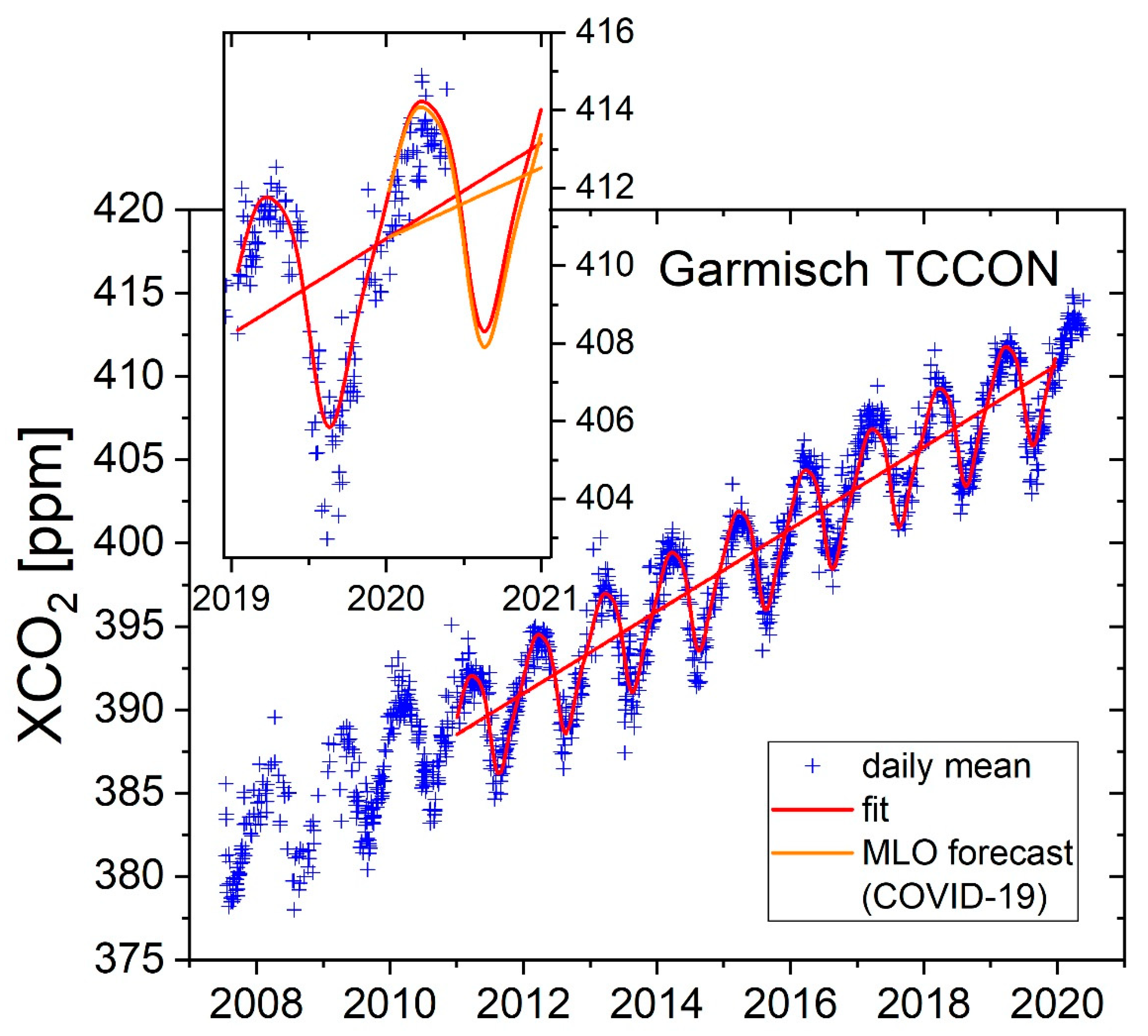
Figure 1 shows the daily-mean XCO2 time series from the Garmisch TCCON site. For the time period (January 2011, December 2019) a mean linear trend of 2.46 [2.44, 2.49] (95% confidence) ppm/yr was derived using the mathematics outlined in Section 2.2. In Table 2, we compared this trend with three further mid-latitude stations; Table 1 gives station details.
We also derived a combined trend for the sites Garmisch, Karlsruhe, and Park Falls. This was performed according to the mathematics outlined in Section 2.2.3 and the results in a combined trend of 2.45 [2.44, 2.47] ppm/yr for the time period (January 2011–Dec 2019). The advantage of combining multi-station trends is reflected in the reduction of the confidence interval by 0.02 ppm/yr relative to Garmisch alone.
The very right-hand side of Figure 1 shows the daily-mean XCO2 observations above Garmisch until the end of May 2020. The latest blue crosses are the highest values measured in the whole Garmisch time series: calculating the monthly mean for April 2020 from our daily observations yields a XCO2 value of 413.4 [413.2, 413.6] (95% confidence) ppm.
The insert in Figure 1 (orange line) is based on a 2020 forecast for Mauna Loa [22], see methods for details: the 2020 annual growth rate for Mauna Loa was forecasted to be reduced by −0.32 ppm yr−2 due to COVID-19. It is worth noting that we defined the 2020 annual growth rate as the annual mean 2020 minus the annual mean 2019. Therefore, assuming for simplicity a COVID-19-related trend changing point at the beginning of 2020 and a subsequent linear trend behavior, the −8% annual emissions reduction scenario [22] would result in a −6.4 ppm reduction towards the end of 2020, see orange line in insert of Figure 1. Note, this orange line is likely to be even steeper in the beginning, considering that daily global emissions decreased by –17% at their peak in early April [6].
3.2. TCCON Annual Growth Rates
3.2.1. Interannual Variability of TCCON Annual Growth Rates
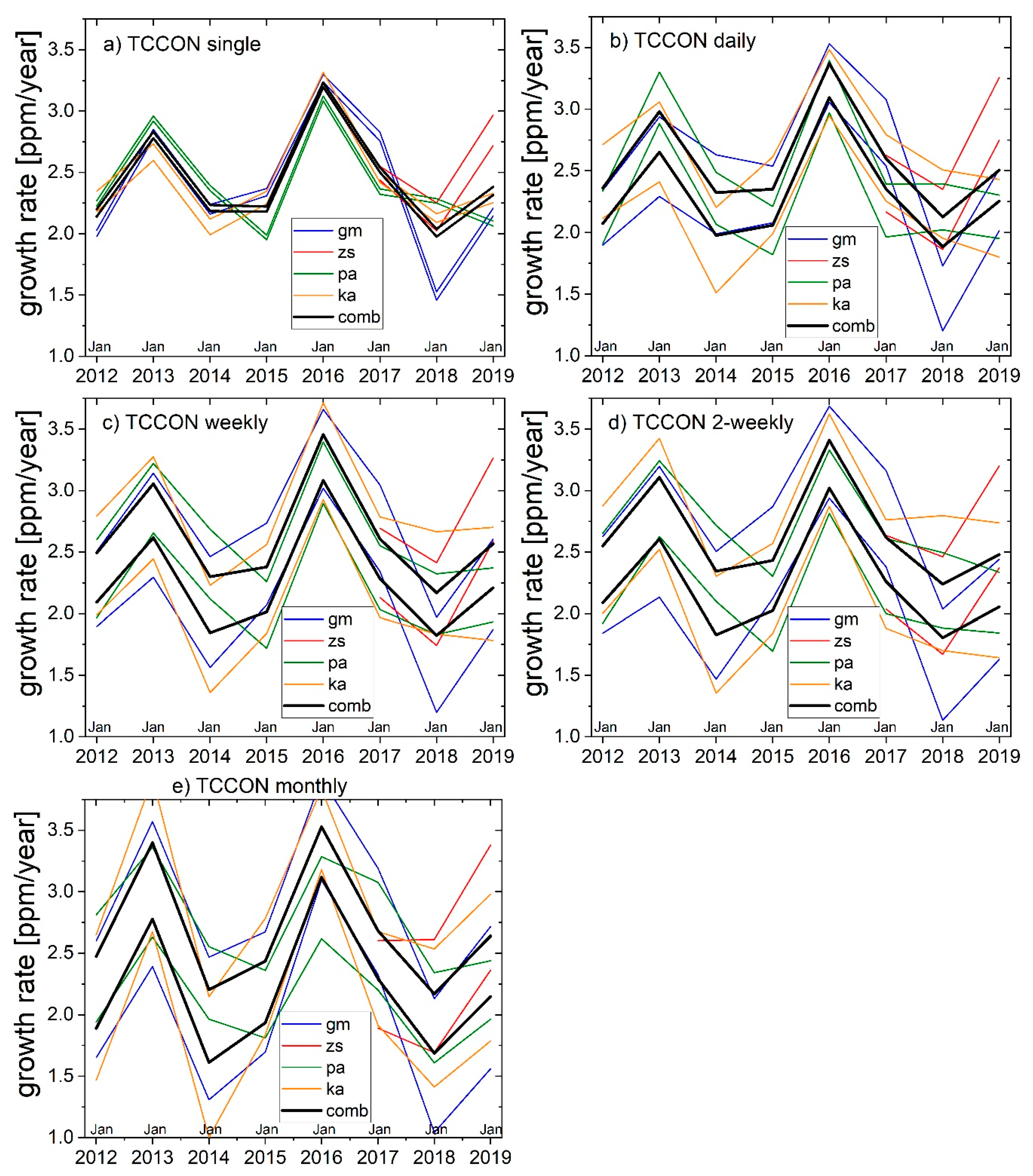
Figure 2 shows the XCO2 annual growth rates covering the years (2012–2019) inferred from the TCCON time series. The analysis for the five sub-figures is based on the time series with differing temporal resolutions: a) using single-spectra time series, b) daily-mean time series, c) is based on weekly-means, d) on 2-weekly means, and e) on monthly means.
The all-sites combined growth rate (black) is 2.44 ppm/yr on overall average over all the years (derived from Figure 2c). There is significant interannual variability: we derived a max–min range of 1.27 ppm/yr from the maximum growth rate of 3.27 ppm/yr achieved in 2016 minus the minimum of 2.00 ppm/yr achieved in 2018. The largest growth rate change within one year is the increase of 1.07 ppm/yr between 2015 (2.20 ppm/yr) and 2016 (3.27 ppm/yr), see Figure 2c.
We point to significant differences between the sites in Figure 2a, which shows a decrease in the annual growth rate from 2018 to 2019 for Park Falls, while the three other stations show an increase. These site differences can be understood considering (i) the differing intra-annual circulations for the differing sites, and (ii) considering that the TCCON operations are limited to clear-sky conditions as follows:
As to (i) we note that even if all TCCON sites were operating 365 days a year, there would be differences in the annual growth rates due to differing circulations: the XCO2 variability relative to the mean seasonal cycle is dominated by synoptic-scale horizontal advection along with the meridional CO2 gradient [20]. A special example for the impact of differing circulation is that the annual growth rates for Zugspitze and Garmisch (sites separated only by ≈8 km horizontal distance) differ in Figure 2a, e.g., in 2018. The mechanism here is that synoptic horizontal advection dominates in the free troposphere relative to the boundary layer where there is less related activity. This is corroborated, e.g., via the observation of two CO2 profiles above Park Falls, while a frontal system moved through the region: the profiles show an increase in free tropospheric CO2 above 5 km by ≈5 ppm, but practically no change below (Figure 6 therein [20]). Due to the altitude difference, the column above Zugspitze (2.96 km asl.) is in the majority of cases fully located within the free troposphere, while the Garmisch column (0.74 km asl.) is not.
As to (ii) we note that even if all sites would encounter the same circulation, differing annual growth rates would result from the data retrieval because each site measures a (differing) under-representation of the circulation (≈100−200 out of 365 days).
Finally, although these site differences tend to become less significant for the widened confidence bands of Figure 2b,d, it is obviously favorable for both reasons (i) and (ii) to not just use one station but the multi-site combination (black lines in Figure 2) in order to obtain hemispherically representative annual growth rates (which is the goal of this study).
3.2.2. Confidence Bands for the TCCON Annual Growth Rates
We consider the case of synoptic scale aggregates of the time series (i.e., daily, weekly, 2-weekly) as the most appropriate basis to estimate the confidence bands for the annual growth rates attainable by TCCON. Taking numbers from Table 3 we will represent this thereafter as follows: 0.38 [0.28, 0.44] ppm/yr, where the 0.38 ppm/yr is obtained from the analysis with weekly-sampling resolution of the time series, the lower range boarder of 0.28 ppm/yr is obtained from the analysis with the daily-sampling resolution of the time series and the upper boarder of 0.44 ppm/yr from the analysis with the 2-weekly resolution.
In the following, we will explain the reasoning behind the choice of synoptic-scale sampling in general, and in particular, why we consider both the confidence band obtained from the fully resolved single-spectra analysis (0.05 ppm/yr, Table 3) and the confidence band obtained from the analysis of the monthly-mean time series (0.51 ppm/yr, Table 3) as unrealistically low and high, respectively.
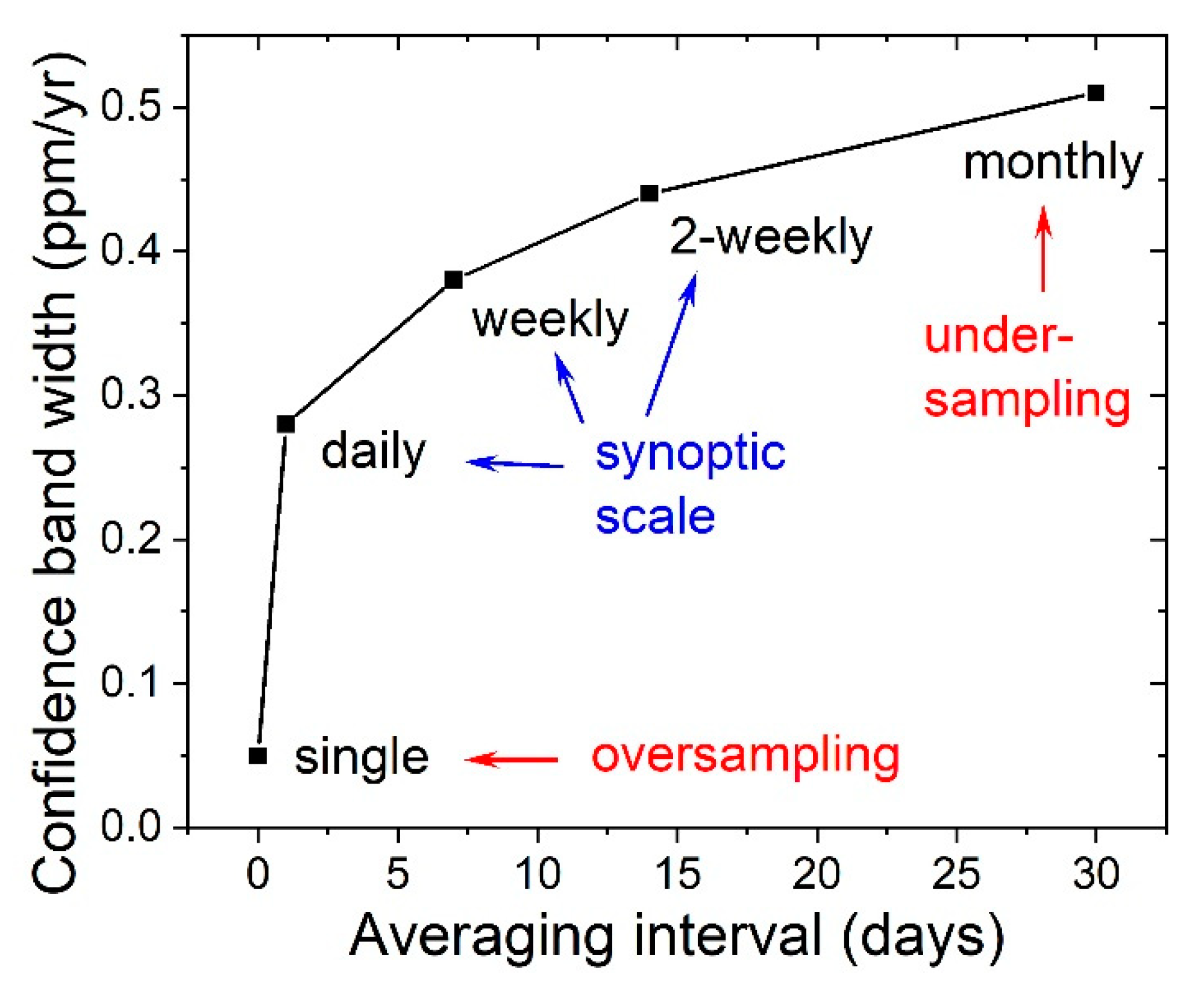
Figure 3 shows the confidence-band width for the annual growth rates retrieved from the TCCON multi-site combination (gm, zs, pa, ka) as a function of the sampling resolution of the underlying TCCON time series. We thereafter discuss three temporal domains: oversampling, synoptic scale sampling, undersampling.
Oversampling with Single-Spectra Resolution
The first data point in Figure 3 for the single-spectra (≈1 min) sampling show the smallest possible confidence band width (0.05 ppm/yr). Figure 2a shows that these confidence bands are often narrower than the differences of annual growth rates between sites, which can be understood as follows.
In the methods Section, we defined the annual growth rate as the difference between the annual mean of a year and the previous year. This means that the growth rate uncertainty is determined by the uncertainty for obtaining annual means. We will show thereafter that the TCCON uncertainty for annual means is neither dominated by the TCCON single measurement precision, nor by local emission histories, but by the intra-annual variability of XCO2 at a certain site over the year, relative to the mean seasonal cycle. As mentioned before, the XCO2 variability relative to the mean seasonal cycle is dominated by the synoptic-scale horizontal advection along with the meridional CO2 gradient and not by the local emission histories [20]. For example, free tropospheric CO2 can vary by 5 ppm due to the overpass of a frontal system. This leads to an oversampling problem, when using fully resolved TCCON single measurements (time resolution ≈1 min).
As outlined in more detail in the methods (Section 2.2.5), the confidence bands are narrower compared to all other cases using longer temporal sampling intervals because we typically record up to more than a hundred XCO2 values per day, and this implies the oversampling of natural variability. It is worth remembering that the dominant contribution to XCO2 intra-annual variability (relative to the mean seasonal cycle) at a TCCON site originates from the synoptic-scale horizontal transport in combination with the meridional gradient of CO2 [20]; i.e., the dominant part of XCO2 variability occurs on synoptic time scales which range from one day up to more than a week.
As discussed in the previous Section, the first reason why we observe in Figure 2a significantly differing growth rates for the differing sites is that the synoptic evolution (circulation) during the year differs for every TCCON site. In other words, even when TCCON would be operating 365 days a year, there were differences between sites—if fully resolved single-spectra time series (≈1 min scale) are used as a basis—because the differing synoptic evolution of the year is fully resolved. We will see in the following, that these synoptic differences between sites can be more and more averaged out (and the confidence bands are widened) by using time series with longer sampling aggregates (daily, weekly, 2-weekly, and monthly means).
The above explanation on oversampling provides a second reason why we see in Figure 2a, in certain years, significantly differing growth rates for differing sites (differences exceeding the confidence bands): the annual means used as input for the growth rate calculations are derived extremely precisely from ≈10000 measurements—but these many measurements are sampled only on ≈100–200 out of 365 days. This means we measure the annual means/annual growth rates very precisely, but for an under-representation of the continuous synoptic evolution of the year. As a consequence, even closely neighbored sites with the same local emission histories may show differences in annual means/annual growth rates just due to the likely case that the time stamps of single measurements as well as the dates of measurement days differ between the sites (e.g., due to the differing local cloud situations limiting solar absorption measurement operations). Again here, we will see in the following that these synoptic differences between sites can be more and more averaged out by using time series with longer sampling aggregates.
Sampling with Synoptic-Scale Temporal Resolution
In Figure 2b, the annual growth rates are calculated from daily aggregates of the TCCON measurements. The confidence bands become broader (see Figure 3; for numbers, see Table 3) but still do not overlap between the sites in all years. Obviously, with the daily-resolution sampling, still part of the synoptic variability on longer time scales (i.e., meteorological events on the weekly and 2-weekly scale) is oversampled, leading still to an underestimation of the confidence bands. Only extending the sampling to weekly aggregates leads to an overlap of the confidence bands for all sites and all years (Figure 2c). This tendency is continued for 2-weekly sampling (Figure 2d and Figure 3).
We note from Table 3 that there were huge site differences in the confidence width for single-spectra sampling (e.g., Zugspitze 0.20 ppm/yr vs. Park Falls 0.04 ppm/yr). However, for preferred synoptic scale (e.g., weekly) sampling, the confidence width between sites becomes nearly equal (Garmisch 0.73 ppm/yr, Karlsruhe 0.82 ppm/yr, Park Falls 0.53 ppm/yr, Zugspitze 0.64 ppm/yr). In particular, we note that the confidence width becomes 0.38 ppm/yr for the all-sites combination (Table 3). These numbers prove the important fact that the multi-site combination gives the benefit of reducing the confidence bands, even if compared to the site Park Falls with the smallest confidence band. This is another reason why we favor for all subsequent analysis the multi-site combination and not just the use of one station.
Undersampling with Monthly-Scale Temporal Resolution
Figure 2e shows the annual growth rates calculated from monthly aggregates of the TCCON measurements. The confidence bands become broader once more, although the increase shown by Figure 3 significantly flattens out after the initial “elbow” seen around the daily scale. This flattening towards the monthly scale occurs because the synoptic scale, dominating intra-annual XCO2 variability, is exceeded. This goes along with an undersampling of the intra-annual evolution; this can be seen from Figure A1: while the 2019 late-summer XCO2 minimum for Park Falls is well captured by all kinds of temporal samplings, it can be clearly seen that the 2018 late-summer minimum was extraordinarily sharp and this could not be captured by monthly-scale sampling resolution. Therefore, we consider the annual growth rates derived from TCCON time series with monthly-sampling resolution as not appropriate for the discussion of the TCCON sensitivity to the COVID-19 impact on CO2.
All in all, the analysis of the width of the confidence bands for the retrievals of annual growth rates from TCCON time series in Figure 2 and Figure 3 tells us the following:
- The confidence bands in Figure 2a provide a measure for a contribution of ≈0.05 ppm/yr resulting from the propagation of single-measurement precision into TCCON-derived annual growth rates, but are no realistic measure for the total annual growth uncertainty (due to the oversampling/underrepresentation of the synoptic evolution).
- The black Figure 2b–d confidence bands from daily, weekly, and 2-weekly TCCON data (i.e., 0.38 [0.28, 0.44] ppm/yr) can be considered as the realistic total uncertainty estimate/range for the hemispherically representative annual growth rates attainable from the TCCON data; it is favorable to base the analysis of annual growth rates on the time series aggregated into synoptic-scale temporal resolution.
- For preferred synoptic-scale sampling, the annual growth rates from sites with differing sampling densities (see Table 1) become consistent (Figure 2). As a result, it makes sense to combine the annual growth rates of various sites to thereby reduce the confidence width as shown in Table 3 (i.e., not only use the site with the densest sampling).
- Aggregating TCCON time series into monthly means leads to an undersampling of the intra-annual XCO2 evolution and thereby to unreliable annual growth rates and too large confidence bands.
3.3. Synopsis of TCCON Annual Growth Rates with Mauna Loa 2020 Forecast
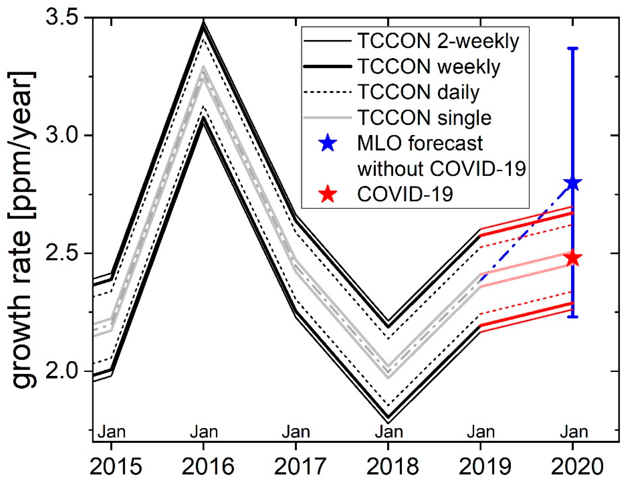
Figure 4 shows the annual growth rates derived from a combination of TCCON stations in the previous Section. Black lines mark a 0.38 [0.28, 0.44] ppm/yr-width confidence band representing the total uncertainty dominated by synoptic-scale variability. The grey band (width 0.05 ppm/yr) is the contribution from the TCCON single-spectra measurement precision. The question is whether this TCCON-related uncertainty allows to detect a COVID-19-related decrease in the growth rate. To answer this, we added a 2020 forecast result [22] to Figure 3, namely 2.8 ppm/yr without the COVID-19 impact (blue star), and 2.48 ppm/yr taking the COVID-19-related emission reductions into account (red star).
These numbers are taken from a May 2020 update [22] of the 2020 forecast of the annual rise in atmospheric carbon dioxide concentration measured at the Mauna Loa, Hawaii (MLO) [36]. A description of this forecast was given in Section 2.3. Briefly, the forecast results indicated in Figure 4 are based on a scenario of a −8% COVID-19-related emission reduction over 2020. In the following, we will refer to the −8% scenario and the derived growth rate forecast [22] to illustrate the size of the potential effects in relation to the TCCON sensitivities.
4. Discussion
4.1. Discussion of Trend Results
The Garmisch trend agrees, within confidence limits, with the trends for Zugspitze, Karlsruhe, and Park Falls (Table 2). It is worth noting that these four northern mid-latitude sites are located within a 3-degree latitude band. The agreement is remarkable, however, since we did not perform any meteorology- or pollution-based data filtering to the measurements. This points to the benefit of the total column observations being representative for wide geographical regions [21].
The combined trend (gm, ka, pa) can be considered as representative for the northern hemisphere. It is consistent with the global mean trend 2.31 [2.29, 2.33] (95% confidence) ppm/yr reported by the global carbon project for the (slightly earlier) time period (2009, 2018) (Table 6 therein [4]): the Garmisch trend for [2011, 2019] is slightly higher, which is well in agreement considering the overall increase in annual growth rates since 2009 (e.g., Figure 8d therein [4]) as well as the increase in the annual growth rate in 2019 in particular (see our Figure 2). Note there are further aspects that potentially contribute to observing slightly differing trends between TCCON and the global carbon project: (i) differing sites—unequal to TCCON the global carbon project uses marine boundary layer stations [4], (ii) TCCON does not measure surface concentrations but column-averaged mole fractions, and (iii) TCCON measurements are restricted to clear-sky conditions.
The April 2020 data shown in Figure 1 represent a new global record high value that has not been exceeded during the past 420,000 years, and likely not during the past 20 million years [39]. The question arises whether we can “see” in these observations COVID-19-related reductions. One obvious qualitative answer from Figure 1 is that there might be a COVID-19 impact in 2020, however, if so, it is not strong enough to turn the anthropogenic XCO2 growth down into a decrease compared to the year 2019. A step-forward working question would therefore be: what amount of reduction in the atmospheric XCO2 increase do we expect from the estimated COVID-19-related emission reductions?
As a crucial conclusion, Figure 1 shows that the forecasted COVID-19 effect is not observable within the variability of the atmospheric observations ranging up to end of May 2020. Therefore, we refined our working question once more, to ask for the rest of this paper: is one year of Total Carbon Column Observations sufficient to significantly detect the forecasted −0.32 ppm yr−2 reduction in the 2020 annual growth rate due to COVID-19? If not, what is the detection delay?
4.2. Discussion of TCCON Annual Growth Rates
In order to approach the question of the short-term sensitivity of TCCON to COVID-19-related changes, we switch now from the concept of multi-annual trends of the last Section to the concept of annual growth rates. While both concepts are a measure for the XCO2 growth with units ppm/yr, we point here to the basic difference: the multi-annual trend can be considered as the multi-annual mean of the annual growth rates; and it is important to note that there is a significant interannual variability of the annual growth rates relative to the mean trend (Figure 4).
The magnitude and reason for these (often quasi-periodic) year-to-year changes of the annual growth rates is briefly discussed: the record high growth rate in 2016 (Figure 4) occurred even though CO2 emissions from fossil fuel consumption and cement production, and the total emissions including deforestation, have been nearly constant between 2014 and 2016. This was caused by a large El Niño event leading to a drying and warming which caused tropical ecosystems to take up less carbon than in other years [2,3]. It is well understood that interannual variability in annual growth rates is dominated by the variability of the ocean and land-vegetation sinks driven by climate variability, while anthropogenic emissions (dominated by fossil fuel emissions) are driving the overall long-term growth of atmospheric CO2 [4].
4.3. Can TCCON Measure a COVID-19-Related Reduction of the Annual Growth Rate? Discussion of Five Cases
We discuss the data behind Figure 4 to investigate the final question of our paper: will TCCON be able to detect a COVID-19-related 2020 growth reduction of (2.48 ppm/yr–2.8 ppm/yr)/1 yr = −0.32 ppm yr−2—given the confidence bands for the TCCON-derived growth rates (red lines in Figure 4), and given the uncertainties of the forecast (blue vertical error bar in Figure 4)? We will elaborate answers to the question of TCCON sensitivity for the five cases summarized in Table 4.
4.3.1. Case (i)
We assumed a one-time 2020 growth rate reduction of −0.32 ppm yr−2, and further assumed that the forecast is true (i.e., zero forecast uncertainty). We used the synoptic scale hemispherically representative TCCON 95% confidence bands (0.38 [0.28, 0.44] ppm/yr from Table 3).
As a proxy for TCCON sensitivity, we derived a “detection delay”. This was inferred from Figure 4 by calculating the intersection point of the upper TCCON confidence line (upper thick red line) for measuring the COVID-19-related forecast (taken as truth), with the forecast line without any COVID-19 impact (dash-dotted blue line). The resulting detection delay was calculated as 0.5 × 0.38 [0.28, 0.44] ppm yr−1/0.32 ppm yr−2 = 0.6 [0.4, 0.7] yr. This number can be interpreted as a measure for the delay contribution of the synoptic variability of XCO2 to the total attainable detection delay. We note that the delay in this case is not limited by the TCCON single-measurement precision (for details, see discussion in Section 3.2.2).
This 0.6 [0.4, 0.7]-yr delay contribution dominated by synoptic variability was directly derived from the analysis of the TCCON data sampled on the synoptic scale, i.e., weekly [daily, 2-weekly] scale. An independent verification/utilization of this 0.6 [0.4, 0.7]-yr TCCON detection capability would require that we knew the forecasted reference case without the COVID-19 impact (i.e., 2.8 ppm/yr for 2020) with zero error—as assumed in our case definition. Obviously, this is not possible. However, verification would become feasible if the forecast confidence band of 2 × 0.57 ppm/yr = 1.14 ppm/yr could be reduced below the TCCON confidence band of 0.38 [0.28, 0.44] ppm/yr. We note that such reduction would require a major evolution step: as can be seen from Figure 4, the currently attainable forecast confidence of 1.14 ppm/yr is only ≈10% narrower than the max–min range of 1.27 ppm/yr measured by TCCON. Clearly, there is room for improvements on the forecast side as stated in previous work [3].
4.3.2. Case (ii)
Same as case (i), however, we now use the TCCON 95% confidence bands for single-spectra data samples (≈1 min time scale, 0.05 ppm/yr from Table 3). Using the TCCON confidence bands for single-spectra resolution, we practically excluded the effect of synoptic variability, and TCCON confidence is limited by single-measurement precision (for details, see discussion in Section 3.2.2).
Again, we derived the detection delay for this case from Figure 4, using the inner confidence band by calculating the intersection point of the upper TCCON confidence line for measuring the COVID-19-related forecast (light red) with the forecast line without the COVID-19 impact (dash-dotted blue line). The resulting detection delay was derived as 0.5 ×0.05 ppm yr−1/0.32 ppm yr−2 = 0.08 yr which is ≈1 month. This number can be interpreted as a measure for the delay contribution of TCCON single-measurement precision to the total attainable detection delay.
The practical verification/utilization of this purely precision-limited ≈ 1 month TCCON detection capability would require that we know the reference case without the COVID-19 impact (i.e., 2.8 ppm/yr for 2020) for the selected set of TCCON sites with a forecast error significantly below 0.05 ppm/yr. This appears not likely to be achievable.
4.3.3. Case (iii)
We assumed a growth rate reduction of −0.32 ppm yr−2 starting in 2020 and assumed to stay constant on this level during the subsequent years. We further assumed forecast uncertainties to apply in the full width of ±0.57 ppm/yr (±2 sigma), as given in [22], see vertical blue error bar indicated in Figure 4 for 2020.
The uncertainty (blue error bar) of the forecasted reference (2.8 ppm/yr, without the COVID-19 impact) is larger than the forecasted growth rate reduction of −0.32 ppm yr−2 taken as truth and to be measured by TCCON (red lines). Therefore, it is obvious from Figure 4, that no significant growth rate reduction can be measured in this case. Of course, the same holds true if the growth rate reduction were limited to 2020 only. The mechanism limiting this (infinite) delay is the forecast uncertainty.
A detection by the end of 2020 would become possible only if the forecast error of ±0.57 ppm/yr could be reduced below ±(0.32 ppm/yr–0.5 × 0.38 [0.28, 0.44] ppm/yr) = ±0.13 [0.10, 0.18] ppm/yr. This seems hardly to be achievable.
4.3.4. Case (iv)
We assumed a growth rate reduction of −0.32 ppm yr−2 starting in 2020 as in the cases before based on a −8% emissions reduction in 2020. However, here we additionally assumed a year-on-year increase in the growth rate reduction by −0.32 ppm yr−2. It is worth noting that this case describes a desirable progressive emission reduction over the years, which may or may not be COVID-19-related after 2020. This is comparable to the emission reductions needed year-on-year over the next decades to limit global warming to 1.5 °C [1]. We further assume a forecast error of ±0.57 ppm/yr and use the TCCON 95% confidence bands for synoptic-scale data samples (0.38 [0.28, 0.44] ppm/yr).
The detection delay for this case was obtained by shifting the blue and red stars to the right while applying the slopes of 2.8 ppm yr−2 (blue) and 2.48 ppm yr−2 (red) until the blue minimum error bar matches the thick red (dashed red, thin red) maximum TCCON confidence line. This resulting detection delay is (0.57 ppm yr−1 + 0.5 × 0.38 [0.28, 0.44] ppm yr−1)/0.32 ppm yr−2 = 2.4 [2.2, 2.5] yr. The dominant mechanisms limiting this delay are the forecast uncertainty, plus an additional smaller contribution from synoptic variability. This detection delay can be interpreted as realistically achievable given the forecast uncertainty attained in [22].
4.3.5. Case (v)
Same as case (iv), but we assumed that there would be no forecast, i.e., there was also no forecast uncertainty. We used the TCCON 95 % confidence bands for the synoptic-scale data samples (0.38 [0.28, 0.44] ppm/yr). In order to derive a detection delay for this case with no forecast uncertainty available, we utilized the 1.27 ppm/yr TCCON max–min range of growth rates from the weekly sampling (2016−2018) derived in Section 3.2.1.
The idea to calculate the detection delay was that due to the progressive growth rate reduction assumed in this case, the growth rate will leave at a certain point the max–min range of the previous observations (which is a rather conservative assumption). The detection delay is therefore calculated as (1.27 ppm yr−1 + 0.38 [0.28, 0.44] ppm/yr)/0.32 ppm yr−2 = 5.2 [4.8, 5.3] yr. The dominant mechanisms limiting this delay were the max–min range of the previous observations with an additional smaller contribution from synoptic variability.
Comparing case (iv) to case (v) indicates that the currently available model forecast helps to reduce the detection delay by a factor of 2.4 yr/5.2 yr ≈ 0.5. Clearly, there is room for improvements on the forecast-side, as stated previously [3].
5. Summary and Conclusions
In spite of the globally significant emission reductions due to the COVID-19 pandemic, we found from the Total Carbon Column Observation Network (TCCON) in April 2020 a historic record high in column-averaged atmospheric carbon dioxide, XCO2. The question of this paper was, whether we could still detect any reduction effects in the atmospheric column concentrations due to COVID-19?
This is a complicated question, because obviously we cannot just measure XCO2 for the reference case without the COVID-19 impact. There is also no point in referencing the growth rate measured the year before. This is because there are large year-to-year growth rate changes which are dominated by climate variability impacting the land and ocean sinks. Anthropogenic emissions and their changes over time, while driving the overall long-term growth of atmospheric CO2, are only a minor contributor to year-to-year changes in the atmospheric growth rate.
The idea to approach this question was, therefore, to explore whether the Total Carbon Column Observations would be able to detect a COVID-19-related reduction of XCO2 relative to a model forecast of the reference case without COVID-19. This included an in-depth analysis of the uncertainties inherent to the TCCON observations and the forecast.
As a tool to pursue this approach, we set up a simple mathematical framework to best possibly derive annual growth rates from the TCCON data given their inhomogeneous sampling (data gaps due to clear-sky conditions). This includes a rigorous derivation of confidence bands which are fully valid for non-normally distributed data like XCO2.
From the subsequent analysis of the TCCON data, we found that the uncertainties of annual XCO2 growth rates are basically given by intra-annual synoptic scale variability, including non-uniform sampling effects (0.38 [0.28, 0.44] ppm/yr, 95% confidence), and by XCO2 measurement precision (0.05 ppm/yr) as a minor contribution.
The basic question of our paper was then addressed by relating the TCCON results to a model forecast of the year 2020 atmospheric growth rate of 2.48 ppm/yr for the scenario of an overall −8% COVID-19-related emissions reduction in 2020—and the forecasted reference case without the COVID-19 impact (2.8 ppm/yr). For example, we assumed a COVID-19-related growth rate reduction of −0.32 ppm yr−2 for 2020 to be true and measured. We then calculated the attainable “detection delay”, i.e., how much time it would take TCCON to measure the “true” 2.48 ppm/yr growth rate until a significant difference vs. the forecasted 2.8 ppm reference case could be obtained given the TCCON confidence and the forecast uncertainty. We thereby obtained the following results:
- (i)
- There is a 0.6 [0.4, 0.7]-yr contribution to the detection delay due to the impact of synoptic variability on XCO2 observations. This was inferred solely from the TCCON data analysis. The forecast-based verification of this result, however, was not feasible. This is because the forecast uncertainty for the forecasted reference case (without the COVID-19 impact) exceeds the forecasted (and to-be-measured) 2020 growth rate reduction. The currently attainable forecast confidence is only ≈10% narrower than the max–min range observed by TCCON during the last 10 years.
- (ii)
- There is a ≈1-month (0.08-yr) contribution to the detection delay, originating from the (0.8 ppm) single-measurement precision of the TCCON measurements on the ≈1 min scale.
- (iii)
- Taking the reported forecast uncertainty of ±0.57 ppm/yr for the forecasted reference case (without the COVID-19 impact) fully into account, a one-time growth rate reduction of −0.32 ppm yr−2 in 2020 cannot be detected. The same holds true if the growth rate reduction would stay constant on the same level during the subsequent years.
- (iv)
- We assumed a growth rate reduction of −0.32 ppm yr−2 starting in 2020, as in the cases before based on a −8 % emissions reduction in 2020. However, we then additionally assumed a year-on-year increase in the growth rate reduction by −0.32 ppm yr−2. This describes a desirable progressive emission reduction over the years, which may or may not be COVID-19 related after 2020. This case is comparable to the rates of decrease needed over the next decades to limit climate change to a 1.5 °C warming. For this case, we derived an overall detection delay of 2.4 [2.2, 2.5] yr. This is limited by the forecast uncertainty with an additional contribution from synoptic variability.
- (v)
- Finally, assuming the same type of progressive growth rate reduction, we investigated the case that no forecast for the reference case (without the COVID-19 impact) would be available. The idea to derive a detection delay was that due to the progressive growth rate reduction assumed, that the growth rate will leave at a certain point the max–min range of the previous observations. The resulting overall detection delay is 5.2 [4.8, 5.3] yr.
In conclusion, we learned from this study that the crucial limitation for verifying the bottom-up estimates of the underlying ≈ −8% emission reductions by atmospheric column measurements is the uncertainty for the required forecasted reference growth rates. We found that the currently attainable forecast confidence band for the growth rates was only ≈10% narrower than the max–min range observed by TCCON during the last decade. Therefore, it remains an important goal to reduce forecast uncertainty. This would require a step forwards in the optimization of the underlying terrestrial ecosystem models to better estimate the variability of the land sink, or significantly improve the ocean observations to better quantify the variability of the ocean sink.
As a final conclusion, the adopted scenario of a COVID-19-related global emissions reduction of −8% in 2020 assumed in this paper may be considered as unprecedented and large. However, the emission reductions of approximately this magnitude have to be continued by policy measures year-on-year over the next decades, independently of COVID-19, in order to keep global warming below 1.5 °C [1]. Obviously, this cannot be attained by COVID-19-like lockdown restrictions; rather, fundamental energy technology changes are required.
As a basis for future research, this paper set up a technical framework and quantified the sensitivity to potentially detect ≈ −8% annual emission reductions (one-time, constant, or cumulating year-on-year) from atmospheric Total Carbon Column Observations, in comparison with an atmospheric reference forecast. Our underlying procedures to robustly calculate annual growth rates require the complete year of atmospheric measurements (along with the complete previous year data). Therefore, in a follow-up study, we will infer the 2020 annual growth rate directly after the turn of the year 2020/21. The plans are to use the full TCCON network with all globally available sites. Ideally, the TCCON-derived annual growth rates will then be compared to a reanalysis of the 2020 forecast, now performed for all the individual TCCON sites, in order to assess whether significant emission reductions have occurred. Repeating this procedure year-on-year will allow to verify whether global policy and society will accomplish to find a way out of fossil fuel use.
Author Contributions
Conceptualization, R.S.; methodology, R.S.; software, M.R.; validation, R.S. and M.R.; formal analysis, R.S. and M.R.; investigation, R.S. and M.R.; resources, R.S.; data curation, M.R.; writing—original draft preparation, R.S.; writing—review and editing, R.S.; visualization, R.S. and M.R..; supervision, R.S.; project administration, R.S.; funding acquisition, R.S. All authors have read and agreed to the published version of the manuscript.
Funding
The TCCON stations Garmisch, Zugspitze, and Karlsruhe have been supported by the European Space Agency (ESA) under grant 4000120088/17/I-EF and by the German Bundesministerium für Wirtschaft und Energie (BMWi) via the DLR under grants 50EE1711A & D. We acknowledge funding by the Helmholtz Society via the research program ATMO and by the KIT-Publication Fund of the Karlsruhe Institute of Technology.
Acknowledgments
The authors are indebted to Coleen Roehl and Paul Wennberg (CALTECH) as well to Thomas Blumenstock and Frank Hase (KIT/IMK-ASF) for making their TCCON data for the sites Park Falls and Karlsruhe available for this study. We thank Hans Peter Schmid (KIT/IMK-IFU) for his continuous interest in this work.
Conflicts of Interest
The authors declare no conflict of interest.
Appendix A
Figure A1.
Park Falls time series aggregated into five differing temporal resolutions, i.e., single-spectra (≈1 min), daily, weekly, 2-weekly, and monthly resolution.
Figure A1.
Park Falls time series aggregated into five differing temporal resolutions, i.e., single-spectra (≈1 min), daily, weekly, 2-weekly, and monthly resolution.

References
- Intergovernmental Panel on Climate Change (IPCC). Global Warming of 1.5 °C. An IPCC Special Report on the Impacts of Global Warming of 1.5 °C above Pre-Industrial Levels and Related Global Greenhouse Gas Emission Pathways, in the Context of Strengthening the Global Response to the Threat of Climate Change, Sustainable Development, and Efforts to Eradicate Poverty; Masson-Delmotte, V., Zhai, P., Pörtner, H.-O., Roberts, D., Skea, J., Shukla, P.R., Pirani, A., Moufouma-Okia, W., Péan, C., Pidcock, R., et al., Eds.; World Meteorological Organization: Geneva, Switzerland, 2018; in press. [Google Scholar]
- Betts, R.A.; Jones, C.D.; Knight, J.R.; Keeling, R.F.; Kennedy, J.J. El Niño and a record CO2 rise. Nat. Clim. Chang. 2016, 6, 806–810. [Google Scholar] [CrossRef]
- Peters, G.P.; Le Quéré, C.; Andrew, R.M.; Canadell, J.G.; Friedlingstein, P.; Ilyina, Z.; Jackson, R.B.; Joos, F.; Korsbakken, J.I.; McKinley, G.A.; et al. Towards real-time verification of CO2 emissions. Nat. Clim. Chang. 2017, 7, 848–852. [Google Scholar] [CrossRef] [Green Version]
- Friedlingstein, P.; Jones, M.W.; O’Sullivan, M.; Andrew, R.M.; Hauck, J.; Peters, G.P.; Peters, W.; Pongratz, J.; Sitch, S.; Le Quéré, C.; et al. Global Carbon Budget 2019. Earth Syst. Sci. Data 2019, 11, 1783–1838. [Google Scholar] [CrossRef] [Green Version]
- Le Quéré, C.; Jackson, R.B.; Jones, M.W.; Smith, A.J.P.; Abernethy, S.; Andrew, R.M.; De-Gol, A.J.; Willis, D.R.; Shan, Y.; Canadell, J.G.; et al. Temporary reduction in daily global CO2 emissions during the COVID-19 forced confinement. Nat. Clim. Chang. 2020. [Google Scholar] [CrossRef]
- The International Energy Agency (IEA). Global Energy Review 2020; IEA: Paris, France, 2020; Available online: https://www.iea.org/reports/global-energy-review-2020 (accessed on 4 June 2020).
- Liu, Z.; Ciais, P.; Deng, Z.; Lei, R.; Davis, S.J.; Feng, S.; Zheng, B.; Cui, D.; Dou, X.; He, P.; et al. COVID-19 causes record decline in global CO2 emissions. arXiv 2020, arXiv:2004.13614v3. [Google Scholar]
- Wunch, D.; Toon, G.C.; Blavier, J.-F.L.; Washenfelder, R.A.; Notholt, J.; Connor, B.J.; Griffith, D.W.T.; Sherlock, V.; Wennberg, P.O. The Total Carbon Column Observing Network. Phil. Trans. R. Soc. A 2011, 369, 2087–2112. [Google Scholar] [CrossRef] [PubMed] [Green Version]
- Wunch, D.; Wennberg, P.O.; Toon, G.C.; Connor, B.J.; Fisher, B.; Osterman, G.B.; Frankenberg, C.; Mandrake, L.; O’Dell, C.; Ahonen, P.; et al. A method for evaluating bias in global measurements of CO2 total columns from space. Atmos. Chem. Phys. 2011, 11, 12317–12337. [Google Scholar] [CrossRef] [Green Version]
- Liang, A.; Gong, W.; Han, G.; Xiang, C. Comparison of Satellite-Observed XCO2 from GOSAT, OCO-2, and Ground-Based TCCON. Remote Sens. 2017, 9, 1033. [Google Scholar] [CrossRef] [Green Version]
- Wunch, D.; Wennberg, P.O.; Osterman, G.; Fisher, B.; Naylor, B.; Roehl, C.M.; O’Dell, C.; Mandrake, L.; Viatte, C.; Kiel, M.; et al. Comparisons of the Orbiting Carbon Observatory-2 (OCO-2) XCO2 measurements with TCCON. Atmos. Meas. Tech. 2017, 10, 2209–2238. [Google Scholar] [CrossRef] [Green Version]
- Wu, L.; Hasekamp, O.; Hu, H.; Landgraf, J.; Butz, A.; aan de Brugh, J.; Aben, I.; Pollard, D.F.; Griffith, D.W.T.; Feist, D.G.; et al. Carbon dioxide retrieval from OCO-2 satellite observations using the RemoTeC algorithm and validation with TCCON measurements. Atmos. Meas. Tech. 2018, 11, 3111–3130. [Google Scholar] [CrossRef] [Green Version]
- O’Dell, C.W.; Eldering, A.; Wennberg, P.O.; Crisp, D.; Gunson, M.R.; Fisher, B.; Frankenberg, C.; Kiel, M.; Lindqvist, H.; Mandrake, L.; et al. Improved retrievals of carbon dioxide from Orbiting Carbon Observatory-2 with the version 8 ACOS algorithm. Atmos. Meas. Tech. 2018, 11, 6539–6576. [Google Scholar] [CrossRef] [Green Version]
- Reuter, M.; Buchwitz, M.; Schneising, O.; Noël, S.; Bovensmann, H.; Burrows, J.P.; Boesch, H.; Di Noia, A.; Anand, J.; Parker, R.J.; et al. Ensemble-based satellite-derived carbon dioxide and methane column-averaged dry-air mole fraction data sets (2003–2018) for carbon and climate applications. Atmos. Meas. Tech. 2020, 13, 789–819. [Google Scholar] [CrossRef] [Green Version]
- Chevallier, F.; Deutscher, N.; Conway, T.J.J.; Ciais, P.; Ciattaglia, L.; Dohe, S.; Fröhlich, M.; Gomez-Pelaez, A.J.; Hase, F.; Haszpra, L.; et al. Global CO2 surface fluxes inferred from surface air-sample measurements and from TCCON retrievals of the CO2 total column. Geophys. Res. Lett. 2011, 38, L24810. [Google Scholar] [CrossRef] [Green Version]
- Reuter, M.; Buchwitz, M.; Hilker, M.; Heymann, J.; Schneising, O.; Pillai, D.; Bovensmann, H.; Burrows, J.P.; Bösch, H.; Parker, R.; et al. Satellite-inferred European carbon sink larger than expected. Atmos. Chem. Phys. 2014, 14, 13739–13753. [Google Scholar] [CrossRef] [Green Version]
- Feng, L.; Palmer, P.I.; Parker, R.J.; Deutscher, N.M.; Feist, D.G.; Kivi, R.; Morino, I.; Sussmann, R. Estimates of European uptake of CO2 inferred from GOSAT XCO2 retrievals: Sensitivity to measurement bias inside and outside Europe. Atmos. Chem. Phys. 2016, 16, 1289–1302. [Google Scholar] [CrossRef] [Green Version]
- Lindqvist, H.; O’Dell, C.W.; Basu, S.; Boesch, H.; Chevallier, F.; Deutscher, N.; Feng, L.; Fisher, B.; Hase, F.; Inoue, M.; et al. Does GOSAT capture the true seasonal cycle of carbon dioxide? Atmos. Chem. Phys. 2015, 15, 13023–13040. [Google Scholar] [CrossRef] [Green Version]
- Yuan, Y.; Sussmann, R.; Rettinger, M.; Ries, L.; Petermeier, H.; Menzel, A. Comparison of Continuous In-Situ CO2 Measurements with Co-Located Column-Averaged XCO2 TCCON/Satellite Observations and CarbonTracker Model Over the Zugspitze Region. Remote Sens. 2019, 11, 2981. [Google Scholar] [CrossRef] [Green Version]
- Keppel-Aleks, G.; Wennberg, P.O.; Washenfelder, R.A.; Wunch, D.; Schneider, T.; Toon, G.C.; Andres, R.J.; Blavier, J.-F.; Connor, B.; Davis, K.J.; et al. The imprint of surface fluxes and transport on variations in total column carbon dioxide. Biogeosciences 2012, 9, 875–891. [Google Scholar] [CrossRef] [Green Version]
- Olsen, S.C.; Randerson, J.T. Differences between surface and column atmospheric CO2 and implications for carbon cycle research. J. Geophys. Res. 2004, 109, D02301. [Google Scholar] [CrossRef] [Green Version]
- Betts, R.A.; Jones, C.D.; Jin, Y.; Keeling, R.F.; Kennedy, J.J.; Knight, J.R.; Scaife, A. Analysis: What Impact Will the Coronavirus Pandemic Have on Atmospheric CO2? CarbonBrief. 2020. Available online: https://www.carbonbrief.org/analysis-what-impact-will-the-coronavirus-pandemic-have-on-atmospheric-co2 (accessed on 4 June 2020).
- Messerschmidt, J.; Geibel, M.C.; Blumenstock, T.; Chen, H.; Deutscher, N.M.; Engel, A.; Feist, D.G.; Gerbig, C.; Gisi, M.; Hase, F.; et al. Calibration of TCCON column-averaged CO2: The first aircraft campaign over European TCCON sites. Atmos. Chem. Phys. 2011, 11, 10765–10777. [Google Scholar] [CrossRef] [Green Version]
- Sussmann, R.; Schäfer, K. Infrared spectroscopy of tropospheric trace gases: Combined analysis of horizontal and vertical column abundances. Appl. Opt. 1997, 36, 735–741. [Google Scholar] [CrossRef] [PubMed]
- Sussmann, R.; Rettinger, M. TCCON Data from Garmisch (DE), Release GGG2014.R2 [Data Set]; TCCON Data Archive, Hosted by CaltechDATA: Pasadena, CA, USA, 2018; R2. [Google Scholar]
- Sussmann, R.; Rettinger, M. TCCON Data from Zugspitze (DE), Release GGG2014.R1 [Data Set]; TCCON Data Archive, Hosted by CaltechDATA: Pasadena, CA, USA, 2018; R1. [Google Scholar]
- Hase, F.; Blumenstock, T.; Dohe, S.; Groß, J.; Kiel, M. TCCON Data from Karlsruhe (DE), Release GGG2014R1. [Data Set]; TCCON Data Archive, Hosted by CaltechDATA: Pasadena, CA, USA, 2015; R1. [Google Scholar] [CrossRef]
- Wennberg, P.O.; Roehl, C.M.; Wunch, D.; Toon, G.C.; Blavier, J.-F.; Washenfelder, R.; Keppel-Aleks, G.; Allen, N.T.; Ayers, J. TCCON data from Park Falls (US), Release GGG2014R1. [Data Set]; TCCON data archive, hosted by CaltechDATA: Pasadena, CA, USA, 2017; R1. [Google Scholar] [CrossRef]
- Masarie, K.A.; Tans, P.P. Extension and integration of atmospheric carbon dioxide data into a globally consistent measurement record. J. Geophys. Res. Atmos. 1995, 100, 11593–11610. [Google Scholar] [CrossRef] [Green Version]
- Gatz, D.F.; Smith, L. The standard error of a weighted mean concentration—I. Bootstrapping vs. other methods. Atmos. Environ. 1995, 29, 1185–1193. [Google Scholar] [CrossRef]
- Gatz, D.F.; Smith, L. The standard error of a weighted mean concentration—II. Estimating confidence intervals. Atmos. Environ. 1995, 29, 1195–1200. [Google Scholar] [CrossRef]
- Gardiner, T.; Forbes, A.; de Mazière, M.; Vigouroux, C.; Mahieu, E.; Demoulin, P.; Velazco, V.; Notholt, J.; Blumenstock, T.; Hase, F.; et al. Trend analysis of greenhouse gases over Europe measured by a network of ground-based remote FTIR instruments. Atmos. Chem. Phys. 2008, 8, 6719–6727. [Google Scholar] [CrossRef] [Green Version]
- Kohlhepp, R.; Ruhnke, R.; Chipperfield, M.P.; De Maziere, M.; Notholt, J.; Barthlott, S.; Batchelor, R.L.; Blatherwick, R.D.; Blumenstock, T.; Coffey, M.T.; et al. Observed and simulated time evolution of HCl, ClONO2, and HF total column abundances. Atmos. Chem. Phys. 2012, 12, 3527–3556. [Google Scholar] [CrossRef] [Green Version]
- Sussmann, R.; Borsdorff, T.; Rettinger, M.; Camy-Peyret, C.; Demoulin, P.; Duchatelet, P.; Mahieu, E.; Servais, C. Harmonized retrieval of column-integrated atmospheric water vapor from the FTIR network-first examples for long-term records and station trends. Atmos. Chem. Phys. 2009, 9, 8987–8999. [Google Scholar] [CrossRef] [Green Version]
- Sussmann, R.; Forster, F.; Rettinger, M.; Bousquet, P. Renewed methane increase for five years (2007–2011) observed by solar FTIR spectrometry. Atmos. Chem. Phys. 2012, 12, 4885–4891. [Google Scholar] [CrossRef] [Green Version]
- Met Office. Mauna Loa Carbon Dioxide Forecast for 2020. Available online: https://www.metoffice.gov.uk/research/climate/seasonal-to-decadal/long-range/forecasts/co2-forecast (accessed on 4 June 2020).
- Kennedy, J.J.; Rayner, N.A.; Smith, R.O.; Parker, D.E.; Saunby, M. Reassessing biases and other uncertainties in sea surface temperature observations measured in situ since 1850: 2. Biases and homogenization. J. Geophys. Res. Atmos. 2011, D14104. [Google Scholar] [CrossRef]
- MacLachlan, C.; Arribas, A.; Peterson, K.A.; Maidens, A.; Fereday, D.; Scaife, A.A.; Gordon, M.; Vellinga, M.; Williams, A.; Comer, R.E.; et al. Global Seasonal forecast system version 5 (GloSea5): A high-resolution seasonal forecast system. Q. J. R. Meteorol. Soc. 2015, 141, 1072–1084. [Google Scholar] [CrossRef]
- Prentice, I.C.; Farquhar, G.D.; Fasham, M.J.R.; Goulden, M.L.; Heimann, M.; Jaramillo, V.J.; Kheshgi, H.S.; Le Quéré, C.; Scholes, R.J.; Wallace, D.W.R. The Carbon Cycle and Atmospheric Carbon Dioxide. In Climate Change 2001: The Scientific Basis, Contribution of Working Group I to the Third Assessment Report of the Intergovernmental Panel on Climate Change; Houghton, J.T., Ding, Y., Griggs, D.J., Noguer, M., van der Linden, P.J., Dai, X., Maskell, K., Johnson, C.A., Eds.; Cambridge University Press: Cambridge, UK; New York, NY, USA, 2001; pp. 183–237. [Google Scholar]
Figure 1.
Daily-mean XCO2 time series for the TCCON site Garmisch. The model fit (red) comprises a linear trend along with a fourth order Fourier series. The insert shows in addition in orange the forecasted trend reduction in 2020 due to COVID-19 [22] along with the tilted seasonal curve.
Figure 1.
Daily-mean XCO2 time series for the TCCON site Garmisch. The model fit (red) comprises a linear trend along with a fourth order Fourier series. The insert shows in addition in orange the forecasted trend reduction in 2020 due to COVID-19 [22] along with the tilted seasonal curve.

Figure 2.
Annual XCO2 growth rates for the TCCON sites Garmisch, Zugspitze, Park Falls, and Karlsruhe. The colored lines indicate the 95% confidence bands retrieved from the bootstrap resampling of the individual sites, and black is the multi-site combination: (a) the analysis based on the single-spectra TCCON data; (b) the analysis based on the daily-mean TCCON data; (c) the analysis based on the weekly-mean TCCON data; (d) the analysis based on the 2-weekly-mean TCCON data; and (e) the analysis based on the monthly-mean TCCON data.

Figure 3.
Width of the 95% confidence bands for the annual growth rates retrieved from the TCCON multi-site combination (gm, zs, pa, ka) as a function of the sampling resolution of the time series: single-spectra (≈1 min), daily, weekly, 2-weekly, and monthly resolution. Underlying data are the last row of Table 3.

Figure 4.
Hemispherically representative annual growth rates derived from a combination of the TCCON sites Garmisch, Zugspitze, Karlsruhe, and Park Falls. The thick black lines give the 95% confidence band derived from the measured time series aggregated into weekly means, the thin black is from the 2-weekly sampling resolution, the dashed black is from daily sampling, the while grey is from using ≈1-min single-spectra sampling. The red and blue stars are the forecasts for Mauna Loa, Hawaii (MLO), with and without the COVID-19 impact [22]. The blue vertical error bars represent 2-sigma forecast uncertainty (±0.57 ppm/yr), and the red lines are the TCCON confidence bands.


Table 1.
Total Carbon Colum Observing Network (TCCON) sites of this study and the sampling characteristics.
Table 1.
Total Carbon Colum Observing Network (TCCON) sites of this study and the sampling characteristics.
| Site | Lat. | Lon. | Alt. (km) | Measurement Days per Year (Average) | Spectra per Day (Average) | Single Spectra Integration Time (s) | Data Set |
|---|---|---|---|---|---|---|---|
| Garmisch (gm 1) | 47°N | 11°E | 0.74 | 127 | 79 | 95 | [25] |
| Zugspitze (zs) | 47°N | 11°E | 2.96 | 110 | 37 | 18/97 2 | [26] |
| Karlsruhe (ka) | 49°N | 8°E | 0.12 | 120 | 46 | 35 | [27] |
| Park Falls (pa) | 46°N | 90°W | 0.44 | 238 | 118 | 95 | [28] |
1 Site indexes used throughout the paper. 2 Before/after 17 Aug 2017.
Table 2.
Trends for the TCCON sites of this study and the combined trend.
| Site | Fitted Period | Trend Slope [ppm/yr] | Confidence Interval [ppm/yr, 95%] |
|---|---|---|---|
| Garmisch | (Jan 2011–Dec 2019) | 2.46 | [2.44, 2.49] |
| Karlsruhe | (Jan 2011–Dec 2019) | 2.46 | [2.43, 2.49] |
| Park Falls | (Jan 2011–Dec 2019) | 2.44 | [2.42, 2.46] |
| Zugspitze | (Jan 2016–Dec 2019) | 2.42 | [2.33, 2.50] |
| Combined (gm, ka, pa) | (Jan 2011–Dec 2019) | 2.45 | [2.44, 2.47] |
Table 3.
Width of the 95% confidence bands for the annual growth rates (mean 2012–2019).
| Site | Monthly (ppm/yr) | 2-Weekly (ppm/yr) | Weekly (ppm/yr) | Daily (ppm/yr) | Single (ppm/yr) |
|---|---|---|---|---|---|
| Garmisch | 1.02 | 0.86 | 0.73 | 0.53 | 0.07 |
| Karlsruhe | 1.03 | 0.91 | 0.82 | 0.60 | 0.10 |
| Park Falls | 0.69 | 0.60 | 0.53 | 0.40 | 0.04 |
| Zugspitze | 0.88 | 0.74 | 0.64 | 0.49 | 0.20 |
| Combined (gm, ka, pa, zs) | 0.51 | 0.44 | 0.38 | 0.28 | 0.05 |
Table 4.
Detection delays for the COVID-19-related XCO2 growth reduction.
| Case (i)−(v) Assumptions | Delay Type | Delay Time (yr) | Data Basis | Dominant Mechanism |
|---|---|---|---|---|
| (i) one-time growth rate reduction 2020 = −0.32 ppm yr−2; forecast error = 0; TCCON confidence (weekly sampling) = 0.38 ppm/yr | delay contribution | 0.6 [0.4, 0.7] | weekly TCCON data | weekly-scale synoptic variability of XCO2 |
| (ii) one-time growth rate reduction 2020 = −0.32 ppm yr−2; forecast error = 0; TCCON confidence (single-spectra sampling) = 0.05 ppm/yr | delay contribution | 0.08 | single-spectra TCCON data | TCCON single-measurement precision |
| (iii) growth rate reduction starting 2020 and constant afterwards = −0.32 ppm yr−2; forecast error = ±0.57 ppm/yr | overall delay | ∞ | forecast error | forecast error |
| (iv) growth rate reduction starting 2020 and linear annual increase afterwards = −0.32 ppm yr−2; forecast error = ±0.57 ppm/yr; TCCON confidence (weekly sampling) = 0.38 ppm/yr | overall delay | 2.4 [2.2, 2.5] | forecast error and weekly TCCON data | forecast error |
| (v) growth rate reduction starting 2020 and linear annual increase afterwards = −0.32 ppm yr−2; no forecast error available; TCCON max–min range (weekly sampling) = 1.27 ppm/yr; TCCON confidence (weekly sampling) = 0.38 ppm/yr | overall delay | 5.2 [4.8, 5.3] | forecast error and weekly TCCON data | observed max–min range of growth rates |
© 2020 by the authors. Licensee MDPI, Basel, Switzerland. This article is an open access article distributed under the terms and conditions of the Creative Commons Attribution (CC BY) license (http://creativecommons.org/licenses/by/4.0/).
Share and Cite
MDPI and ACS Style
Sussmann, R.; Rettinger, M. Can We Measure a COVID-19-Related Slowdown in Atmospheric CO2 Growth? Sensitivity of Total Carbon Column Observations. Remote Sens. 2020, 12, 2387. https://0-doi-org.brum.beds.ac.uk/10.3390/rs12152387
AMA Style
Sussmann R, Rettinger M. Can We Measure a COVID-19-Related Slowdown in Atmospheric CO2 Growth? Sensitivity of Total Carbon Column Observations. Remote Sensing. 2020; 12(15):2387. https://0-doi-org.brum.beds.ac.uk/10.3390/rs12152387
Chicago/Turabian StyleSussmann, Ralf, and Markus Rettinger. 2020. "Can We Measure a COVID-19-Related Slowdown in Atmospheric CO2 Growth? Sensitivity of Total Carbon Column Observations" Remote Sensing 12, no. 15: 2387. https://0-doi-org.brum.beds.ac.uk/10.3390/rs12152387
Note that from the first issue of 2016, this journal uses article numbers instead of page numbers. See further details here.