Hierarchical Sparse Subspace Clustering (HESSC): An Automatic Approach for Hyperspectral Image Analysis

Abstract

Hyperspectral imaging techniques are becoming one of the most important tools to remotely acquire fine spectral information on different objects. However, hyperspectral images (HSIs) require dedicated processing for most applications. Therefore, several machine learning techniques were proposed in the last decades. Among the proposed machine learning techniques, unsupervised learning techniques have become popular as they do not need any prior knowledge. Specifically, sparse subspace-based clustering algorithms have drawn special attention to cluster the HSI into meaningful groups since such algorithms are able to handle high dimensional and highly mixed data, as is the case in real-world applications. Nonetheless, sparse subspace-based clustering algorithms usually tend to demand high computational power and can be time-consuming. In addition, the number of clusters is usually predefined. In this paper, we propose a new hierarchical sparse subspace-based clustering algorithm (HESSC), which handles the aforementioned problems in a robust and fast manner and estimates the number of clusters automatically. In the experiment, HESSC is applied to three real drill-core samples and one well-known rural benchmark (i.e., Trento) HSI datasets. In order to evaluate the performance of HESSC, the performance of the new proposed algorithm is quantitatively and qualitatively compared to the state-of-the-art sparse subspace-based algorithms. In addition, in order to have a comparison with conventional clustering algorithms, HESSC’s performance is compared with K-means and FCM. The obtained clustering results demonstrate that HESSC performs well when clustering HSIs compared to the other applied clustering algorithms.

1. Introduction

Hyperspectral imaging techniques enable the acquisition of hundreds of narrow spectral bands per pixel, covering (based on their sensor characteristics) the spectrum range of visible to near-infrared (VNIR, 0.4–1 μm), shortwave infrared (SWIR, 1–2.5 μm), and longwave infrared spectra (LWIR, 8–13 μm) [1,2]. By using such fine spectral information, accurate discrimination of different materials and objects is possible, which makes hyperspectral images (HSIs) a great source of information for a wide variety of applications such as land-cover classification [3,4] and mineral mapping [5,6,7].

The analysis of HSI is, however, a challenging task due to a number of reasons, such as (1) the inherently nonlinear relations between the captured spectral information and the corresponding material, (2) the existence of high dimensionality (also known as bands) and a limited number of corresponding representative samples, which leads to the so-called the curse of dimensionality [8], (3) the existence of huge redundancy among adjacent bands, and (4) the presence of mixed pixels and different noise types in the data [9].

In order to cope with the aforementioned challenges and process HSIs, several machine learning techniques have been proposed in the past decades. Among the developed machine learning techniques, supervised classification techniques perform well to classify HSIs in different applications [10,11,12]. Nevertheless, for the classification of HSIs, fully supervised algorithms use a set of representative samples of each class, which are also known as training samples. In most cases, acquiring training samples is expensive and time-consuming. Therefore, unsupervised learning techniques (also known as clustering techniques), which classify input data without any label, have drawn considerable attention in many domains, such as computer vision, pattern recognition, and data mining [13].

Traditional clustering algorithms (e.g., K-means and fuzzy c-means (FCM)) normally use distance measures between data points to group them into clusters. For instance, K-means utilizes the Euclidean distance to measure the similarity between data points; data points with small Euclidean distances are grouped into the same cluster [14]. However, in the traditional algorithms, the number of dimensions of subspaces needs to be defined prior to beginning the processing of an HSI. Moreover, the performance of such algorithms is not stable due to the random initialization [15].

Inspired by the sparse coding mechanism of human vision systems [16], sparse representation was developed as a powerful approach for a variety of computer vision tasks, including face recognition, image super-resolution, and data segmentation, to name a few [17,18]. The concept of sparse representation has also been successfully extended to deal with the challenging task of hyperspectral image classification [19,20,21]. For the case of sparse representation classification (SRC), an input signal (i.e., usually a pixel vector) is represented by a sparse linear combination of samples (atoms) from a dictionary [22], in which the existing training data are usually used to produce the dictionary. SRC usually comes with the important advantage of avoiding the heavy and expensive training procedure that a typical supervised classifier generally conducts, since it is performed directly on the dictionary [12].

In [19], Chen et al. proposed a pixel-wise sparse model to classify HSIs in a supervised way. The method assumes that spectral pixels can be approximately represented into a lower-dimensional subspace spanned by dictionary atoms from the same class. To further improve the performance of the spectral classifier and produce classification maps with higher quality, spatial information was incorporated into the classification framework in [19], shaping the joint sparse model (JSM). This method has been improved by developing a number of classification techniques based on the sparse representation model [22,23,24,25]. Although the concept of sparse representation has been maturely developed to deal with supervised problems, it still remains in its infancy for unsupervised problems where there are no training data to shape the dictionary for sparse classification.

In the last decade, sparse subspace-based clustering algorithms have been successfully applied in order to analyze HSIs [15,26,27,28,29]. For instance, in [15], Elhamifar et al. proposed an unsupervised learning algorithm called sparse subspace clustering (SSC). In SSC, the entire dataset is used to identify the number of subspaces and data points that belong to each subspace. Although SSC provides good clustering results, one of its drawbacks is that it demands more time and computational power to process larger datasets.

In [30], the authors proposed a sparse subspace clustering algorithm by orthogonal matching pursuit (SSC-OMP). SSC-OMP uses the orthogonal matching pursuit algorithm as a greedy feature selection method to compute the sparsest coefficients in the sparse optimization problem. Consequently, the computed sparse coefficient matrix is used to cluster the data [31]. However, in such an algorithm the number of clusters has to be defined in advance.

In [26], the authors proposed exemplar-based subspace clustering (ESC), which is regarded as a fast sparse subspace-based algorithm to cluster large datasets. ESC is employed in order to cluster all of the data by using some representative samples. Due to the use of a few numbers of samples to shape the dictionary, ESC is able to analyze larger datasets within an acceptable processing time. In ESC, in order to define the subset of representative samples, the first sample of the subset is randomly selected, and based on that the other samples will be selected. Although ESC can efficiently handle the data, there are some limitations to its concepts. In ESC, there is no criterion to chose the first sample of the subset, which leads to an increase in the uncertainty of the algorithm. In other words, the algorithm is not stable due to the random selection of the first sample in the subset of representative samples. Besides, in ESC, the number of clusters has to be predefined.

In [32], Wu et al. proposed a hierarchical sparse subspace clustering algorithm to cluster the datasets at multiple resolutions. The proposed algorithm by Wu et al. is able to classify the data in a semi-automatic way, and it can be useful for obtaining information at different resolutions. Nonetheless, it can be time-consuming since it uses SSC in each node of the hierarchical structure to cluster the data, which significantly reduces the efficiency of the algorithm.

In this paper, to address the aforementioned challenges, we propose a new hierarchical sparse subspace-based clustering algorithm to analyze the HSI. The proposed algorithm has the capability of handling large datasets in a fast and robust manner. In the proposed algorithm, a hierarchical structure is used to analyze the data at different levels of detail. The foundation of the hierarchical structure is a lasso-based binary clustering algorithm, in which, to accelerate the clustering analysis, a random sample is selected to proceed with the binary clustering procedure. To reduce the random selection effect, an entropy-based ensemble algorithm is employed [33]. Additionally, in order to have an automatic manner to generate the number of clusters, a criterion is defined by comparing the calculated reconstruction error values at parental and child nodes. At the final step, a label is assigned to each end-node to produce the final clustering map. Thus, we can summarize the contribution of our proposed algorithm as follows:

• We propose a sparse subspace-based clustering algorithm that considerably reduces the computational power requirements by using a novel lasso-binary clustering algorithm.
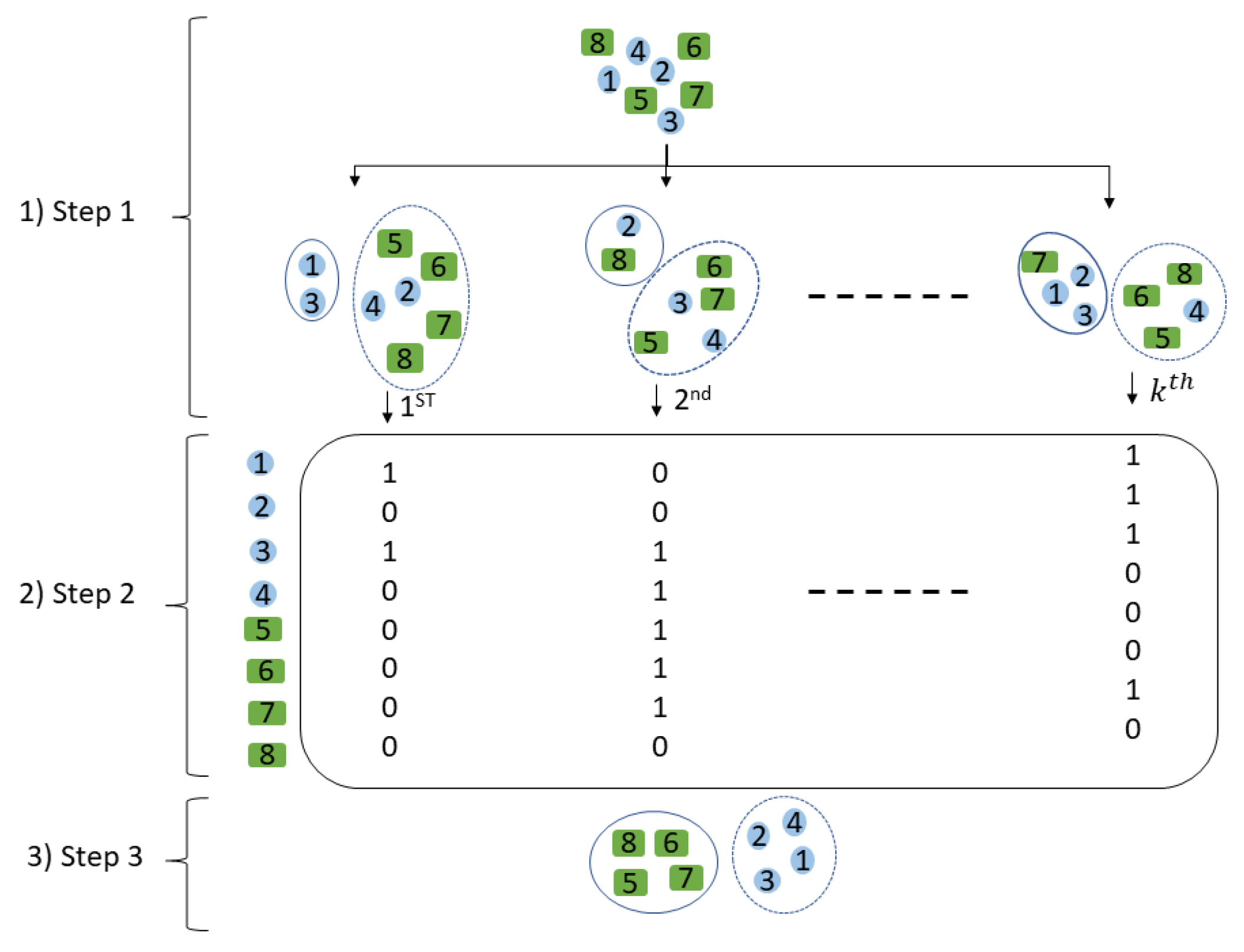
• The proposed algorithm is able to provide robust and stable results thanks to the incorporation of the entropy-based consensus algorithm within its structure, which decreases the effect of the initial random selection of a sample in the lasso-binary clustering algorithm.
• The proposed algorithm benefits from defined criteria, which make it possible to automatically generate the number of clusters.

The paper is organized as follows. The state-of-the-art sparse subspace-based algorithms and the proposed algorithm are elaborated in Section 2. Afterward, the experimental results are presented and discussed in Section 3. Finally, Section 4 is devoted to conclusions and remarks.

2. Methodology

In the following section, an overview of the state-of-the-art subspace clustering algorithms (e.g., scalable exemplar-based subspace clustering [26]) is provided. The proposed clustering algorithm (HESSC) is then elaborated in detail. The workflow of the proposed algorithm is presented in Figure 1.

2.1. Overview on the State-of-the-Art Sparse Subspace-Based Clustering Algorithm

In order to smoothly grasp the concept of the proposed algorithm, we start by introducing the sparse dictionary learning concept. Let us denote $\mathbf{Y}={[{\mathbf{y}}_1,{\mathbf{y}}_2,\dots ,{\mathbf{y}}_N]}^T\in {\mathbb{R}}^{\mathcal{D}\times N}$ as the HSI, where N is the number of pixels and $\mathcal{D}$ is the number of spectral bands in $\mathbf{Y}$. ${\mathbf{y}}_i={[y_{i1},y_{i2},\dots ,y_{i\mathcal{D}}]}^T$ represents the measured spectrum of the i-th pixel in $\mathbf{Y}$, and $i\in \{1,2,\dots ,N\}$ is the pixel indices in the HSI. Let us assume that $\mathbf{Y}$ is free of any kind of error (e.g., noise, measurement failures, etc.), to ease the explanation. In dictionary learning problems, each ${\mathbf{y}}_i$ can be represented by a linear or affine combination of a few atoms from a spectral dictionary $\mathbf{A}=[{\mathbf{a}}_1,{\mathbf{a}}_2,\dots ,{\mathbf{a}}_h]\in {\mathbb{R}}^{\mathcal{D}\times h}$, where $\mathbf{A}$ is a spectral dictionary composed of h spectra that is defined in advance [34]. The aforementioned representation can be formulated as below:

$${\mathbf{y}}_i=\mathbf{A}{\mathbf{c}}_i,$$

(1)

where ${\mathbf{c}}_i=[c_{i1},c_{i2},\dots ,c_{ih}]\in {\mathbb{R}}^h$ is the representation coefficient vector of signal ${\mathbf{y}}_i$. One can also transform Equation (1) into a matrix form as follows:

$$\mathbf{Y}=\mathbf{A}\mathbf{C},$$

(2)

where $\mathbf{C}=[{\mathbf{c}}_1,{\mathbf{c}}_2,\dots ,{\mathbf{c}}_N]\in {\mathbb{R}}^{h\times N}$ is the sparse coefficient matrix that can represent a collection of data points. However, $\mathbf{A}$ is usually over-complete, which results in an ill-posed problem. There are many ways to deal with the ill-posed problem [34,35,36,37]. One of them is to employ the principle of sparsity [15], in which the sparse coefficient matrix can be obtained by solving the following optimization problem:

$$\begin{array}{c}\underset{\mathbf{C}}{min}{\left|\right|\mathbf{C}\left|\right|}_0\hfill \\ S.t.,\mathbf{Y}=\mathbf{AC},\hfill \end{array}$$

(3)

where ${\left|\right|\mathbf{C}\left|\right|}_n$ is the ${\ell }_n$-norm of $\mathbf{C}$, which can be computed as ${\left|\right|\mathbf{C}\left|\right|}_n={\Sigma }_{i=1}^N({\Sigma }_{j=1}^N|c_{ij}{{|}^n)}^{\frac{1}{n}}$ [15]. In Equation (3), ${\ell }_0$-norm represents the number of nonzero elements in $\mathbf{C}$. The problem in Equation (3) is an NP-hard problem, which can be solved by a greedy algorithm (i.e., basis pursuit). However, such an algorithm leads to sub-optimal solutions [38]. In order to deal with the NP-hard problem situation, ${\ell }_0$-norm is replaced with ${\ell }_1$-norm in Equation (3), which is the closest convex approximation of ${\ell }_0$-norm. Therefore, one can rewrite Equation (3) as the following convex problem:

$$\begin{array}{c}\underset{\mathbf{C}}{min}{\left|\right|\mathbf{C}\left|\right|}_1\hfill \\ S.t.,\mathbf{Y}=\mathbf{AC},\hfill \end{array}$$

(4)

Sparse subspace clustering (SSC) is one of the most widely used subspace-based clustering algorithms [26]. In SSC [15], the self-expressiveness property of the data implies that each data point can be written as a linear combination of other data points from the same subspace. In other words, dictionary $\mathbf{A}$ in Equation (4) is replaced with $\mathbf{Y}$. Moreover, we assume that the data points in $\mathbf{Y}$ can be drawn from a union of H linear subspaces, which can be denoted as ${\left\{{\mathcal{S}}_h\right\}}_{h=1}^H$ with respective dimensions ${\left\{d_h\right\}}_{h=1}^H$. Therefore, we can present the $\mathbf{Y}$ as $\mathbf{Y}={\mathbf{Y}}_1\cup {\mathbf{Y}}_2\cup {\mathbf{Y}}_3\cup \dots \cup {\mathbf{Y}}_H$, where each ${\mathbf{Y}}_h\in {\mathbb{R}}^{\mathcal{D}\times N_h}$ is a sub-matrix of $\mathbf{Y}$ consisting of $N_h$ pixels from the ${\mathcal{S}}_h$ subspace (it is also assumed that $N_h>d_h$). The main aim of subspace modeling is to identify the underlying subspaces by using $\mathbf{Y}$. Therefore, the sparse optimization problem in the affinity form can be written as:

$$\begin{array}{cc}\hfill & \underset{\mathbf{C}}{min}{\left|\right|\mathbf{C}\left|\right|}_1\hfill \\ \hfill S.t.,\mathbf{Y}=\mathbf{YC}& ,diag\left(\mathbf{C}\right)=\mathbf{0},{\mathbf{C}}^T\mathbf{1}=\mathbf{1},\hfill \end{array}$$

(5)

where the constraint $diag\left(\mathbf{C}\right)=\mathbf{0}$, $\mathbf{C}\in {\mathbb{R}}^{N\times N}$ is imposed in order to avoid representing a data point as a linear combination of itself. Besides, ${\mathbf{C}}^T\mathbf{1}=\mathbf{1}$ is a constraint to make sure that it is a case of an affine subspace. $\mathbf{1}$ is a vector that consists of one in all elements. The optimization problem in Equation (5) can be solved by employing the alternating direction method of multipliers (ADMM). In order to have a better understanding of the ADMM solver, we refer the interested readers to [39,40]. After obtaining the sparsest coefficient matrix from data points, the symmetrical non-negative similarity matrix $\mathbf{W}\in {\mathbb{R}}^{N\times N}$ is calculated as $\mathbf{W}=\left|\mathbf{C}\right|+{\left|\mathbf{C}\right|}^T$. $\mathbf{W}$ needs to be symmetrical to assure that all nodes from the same subspace are connected to each other. In the last step of SSC, a spectral clustering is applied to the similarity matrix to generate the final clustering result [15]. Although SSC provides reliable results, the algorithm suffers from memory shortage, since SSC employs all data points from $\mathbf{Y}$ to solve the sparse optimization problem in Equation (5). This issue leads to a very high computational time in large datasets [26].

The sparse subspace-based clustering algorithm by orthogonal matching pursuit (SSC-OMP) is a sparse subspace-based algorithm that uses OMP in order to solve the optimization problem in Equation (5). In SSC-OMP, it is assumed that data are contaminated by noise. In order to solve Equation (5), a data point is selected that maximizes the multiplication of the absolute value and the residual [31]. Therefore, SSC-OMP can be written as:

$$\begin{array}{cc}\hfill \underset{\mathbf{C}}{min}& {\left|\right|\mathbf{C}\left|\right|}_1\hfill \\ \hfill S.t.,\left|\right|\mathbf{Y}-{\mathbf{YC}\left|\right|}_F^2& <\mathcal{K},diag\left(\mathbf{C}\right)=\mathbf{0},\hfill \end{array}$$

(6)

where $\mathcal{K}$ shows the number of selected data points from $\mathbf{Y}$ that are used to compute the sparsest coefficients [31]. $\mathcal{K}$ is selected based on the existing noise in the data [30]. The computation of $\mathbf{C}$ in Equation (6) is followed by computing $\mathbf{W}$, and at the last step, the spectral clustering is applied on $\mathbf{W}$ [31]. However, the number of clusters should be known in advance. Additionally, the identification of $\mathcal{K}$ can be crucial as well.

Another recent advanced sparse subspace-based clustering algorithm is the exemplar-based subspace clustering (ESC). In [26], ESC was proposed by You et al. to cope with the scalability problem of SSC in large datasets. In ESC, some representative samples (also known as “exemplars”) are selected to compute the sparsest coefficient matrix, for which the first sample of the representative samples is randomly chosen. The optimization problem in ESC can be formulated as follows:

$$\underset{\mathbf{C},{\mathcal{Y}}_{\mathbf{0}}}{min}{\left|\right|\mathbf{C}\left|\right|}_1+\frac{\lambda }{2}\left|\right|\mathbf{Y}-{\mathcal{Y}}_0\mathbf{C}{\left|\right|}_F^2,$$

(7)

where the sparse coefficient matrix is $\mathbf{C}\in {\mathbb{R}}^{P\times N}$, $\lambda$ is a trade-off parameter between the sparsity and the fidelity terms, and ${\mathcal{Y}}_0=[{\mathbf{y}}_1,{\mathbf{y}}_2,\dots ,{\mathbf{y}}_P]\in {\mathbb{R}}^{\mathcal{D}\times P}$ is a subset of selected representative samples (“exemplars”) from $\mathbf{Y}$, in which P ($P\in \mathbb{Z}$ and $P<<N$) needs to be predefined in advance. In order to compute $\mathbf{C}$ in Equation (7), the lasso version of the LARS algorithm is used [41,42]. Due to the dimension of the computed $\mathbf{C}$ in Equation (7), to achieve the final clustering map, the spectral clustering step is applied to the similarity matrix $\mathbf{W}\in {\mathbb{R}}^{N\times N}$, which is calculated using the t-nearest neighbors of each ${\mathbf{c}}_i$ [26,43]. In ESC, ${\mathcal{Y}}_0$ is used as a dictionary to solve the minimization problem in Equation (7). Therefore, the processing time will be efficiently reduced by using a subset of data points instead of using the entire data. In addition, to the best of our knowledge, ESC has not been investigated yet to analyze HSIs. Although ESC is capable of handling relatively large datasets in a fast manner, its concept suffers from a shortcoming; as mentioned before, in ESC, the first sample of the subset ${\mathcal{Y}}_0$ is randomly selected. Subsequently, the rest of the representative samples are identified by using the farthest first search method proposed in [26], which employs Equation (7) as the cost function. As a result of the random selection of the first sample in ${\mathcal{Y}}_0$, the algorithm reliability is jeopardized. In addition, in ESC, the selection of P is another drawback, since selecting the appropriate number of representative samples has a strong impact on the final clustering result.

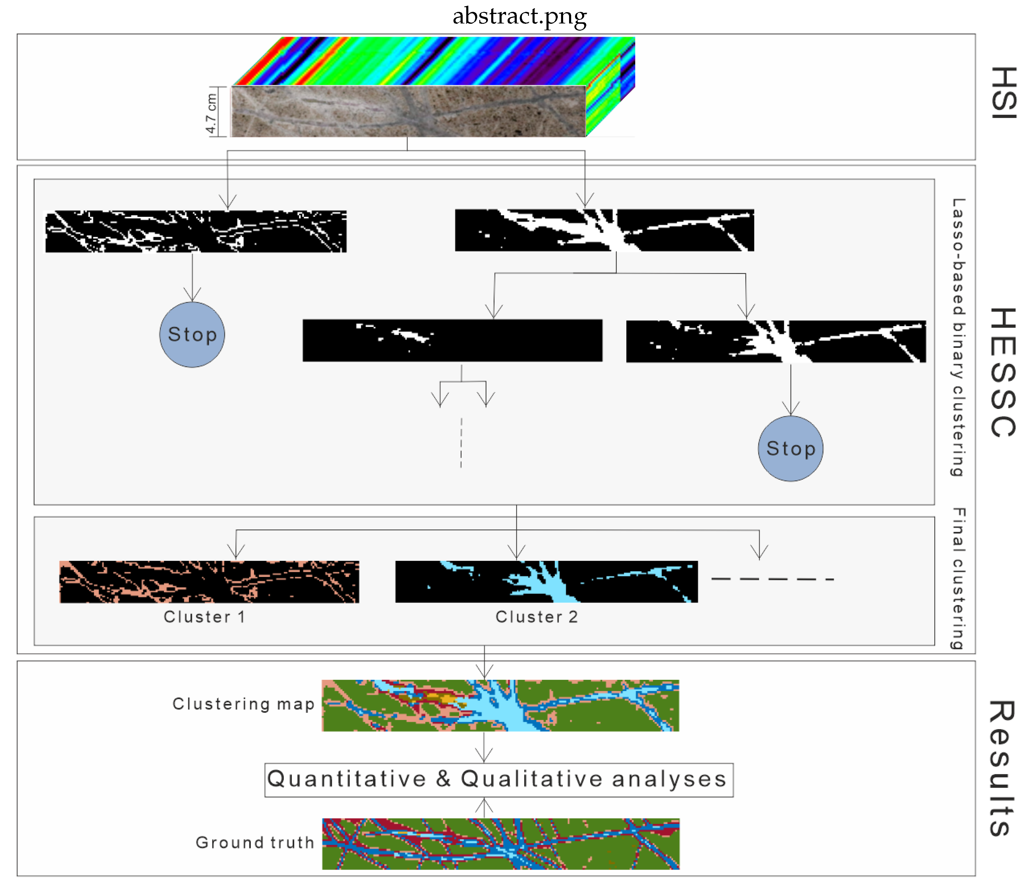
2.2. Hierarchical Sparse Subspace Clustering (HESSC)

In this subsection, the proposed algorithm is described in detail. The approach involves the following three phases: (1) Hierarchical structure (a tree), which allows retrieving information from the HSI at different levels (see Figure 2); (2) Lasso-based binary clustering, which is the core part of the HESSC structure, and is applied to the existing data points at each node of the tree (see Figure 3); (3) Criterion definition, which will be described in detail in Section 2.2.3, which decides whether the current node can be split further or not. Using this criterion in the third phase of HESSC, it is possible to automatically generate the suitable number of clusters for the analyzed dataset. The clusters returned by the algorithm are defined by the leaves of the hierarchical structure, which are the nodes that are not split any further. Specifically, the data points associated with these nodes define the final clusters.

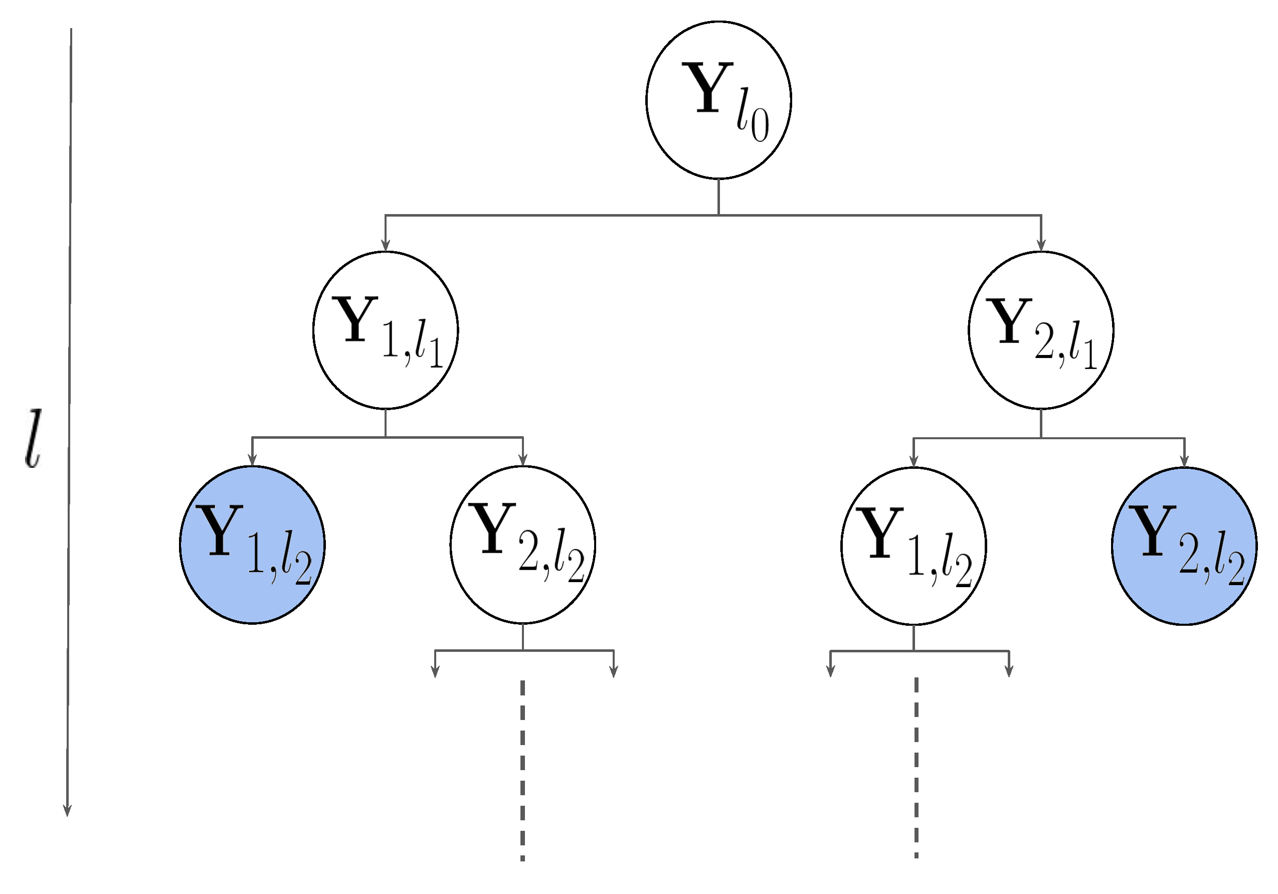
2.2.1. Hierarchical Structure in HESSC

Let us denote the set of data points associated with the r-th node of the b-th level ($l_b$) of the tree as ${\mathbf{Y}}_{r,l_b}$, where $r=\{1,2\}$, $b\in \{0,1,\dots ,l\}$, and l is a user-defined parameter that specifies until what level the HSI needs to be explored, and indirectly defines the upper boundary of the number of clusters in HESSC ($2^l$). ${\mathbf{Y}}_{r,l_b}$ consists of $N_{r,l_b}$ pixels with $N_{r,l_b}<N$. In HESSC, a tree-based data structure is established to describe the existing variation of data points in the HSI at different levels of detail [32]. Additionally, HESSC decreases the computational cost by dividing the data into smaller subsets at each node. As shown in Figure 2, the first node is associated with the original HSI (${\mathbf{Y}}_{l_0}=\mathbf{Y}$). Subsequently, the binary clustering algorithm (Figure 3) is applied to ${\mathbf{Y}}_{l_0}$ to split the ${\mathbf{Y}}_{l_0}$ related with the current node into two groups denoted as ${\mathbf{Y}}_{1,l_1}$ and ${\mathbf{Y}}_{2,l_1}$, which are the two nodes at the first level. In mathematical terms, it is equivalent to ${\mathbf{Y}}_{l_0}={\mathbf{Y}}_{1,l_1}\cup {\mathbf{Y}}_{2,l_1}$. As a result, the split procedure of each node continues until the tree reaches its maximum level, where the number of end-nodes without any constraints on them is equal to $2^l$, or the defined criterion in HESSC is satisfied (see Section 2.2.3). Nonetheless, the entire aforementioned procedure relies on the main idea behind HESSC, which is the lasso-based binary clustering. After obtaining the binary clustering result in the current node, based on the defined criterion, the decision for dividing the current node is made.

2.2.2. Binary Clustering in HESSC

The core of the proposed approach is a binary clustering algorithm, which is based on the lasso-function. The sparse optimization problem in HESSC is equivalent to the ESC minimization problem as shown in Equation (7). Thus, one can write the optimization problem for HESSC as follows:

$$\underset{\mathbf{C}}{min}{\left|\right|\mathbf{C}\left|\right|}_1+\frac{\lambda }{2}\left|\right|{\mathbf{Y}}_{r,l_b}-{\overline{\mathbf{y}}}_i\mathbf{C}{\left|\right|}_F^2,$$

(8)

where $\mathbf{C}\in {\mathbb{R}}^{1\times N_{r,l_b}}$ stands for the computed sparse coefficients, which are equivalent to ${\mathbf{c}}_i$ in Equation (8), and ${\overline{\mathbf{y}}}_i$ is a randomly selected sample from ${\mathbf{Y}}_{r,l_b}$. The main difference between the optimization problem in Equations (7) and (8) is that, in HESSC, instead of having a subset of representative samples, a random sample ${\overline{\mathbf{y}}}_i$ is used to solve the sparse optimization problem. In ESC, the execution time tends to be slower by increasing P, while in Equation (8), the processing time needed to solve the optimization problem is less than the optimization problem associated with Equation (7). The computational burden of the optimization problem in Equation (8) is considerably reduced, since only one random sample is selected to solve the sparse optimization problem. Since ${\overline{\mathbf{y}}}_i$ is randomly chosen, to reduce the randomness effect in the binary clustering procedure, HESSC employs an entropy-based consensus clustering algorithm (ECC), which was proposed in [33]. To the best of our knowledge, this is the first attempt to use ECC in the HSI analysis framework. ECC initially uses a basic clustering algorithm (e.g., K-means) to obtain k distinct clustering results (different groups of the dataset) by varying the number of clusters. Subsequently, ECC employs Shannon entropy as the utility function in order to quantify the similarity between two clustering results (the higher the value of the utility function, the closer the two clustering results are to each other) and looks for the ensemble clustering that has the maximum similarity with all k clustering outputs resulting from the basic clustering algorithm. In order to implement ECC, a modified distance K-means algorithm was developed to obtain the final clustering map [33]. In [33], the execution time can be increased by increasing one of the following parameters: (1) The number of iterations, I, within the ECC algorithm; (2) The number of clustering outputs, which is expressed as k; the outputs are concatenated to be used as entries to ECC; and (3) $\mathcal{L}$, which is the number of clusters in the HSI. Although in HESSC, parameter $\mathcal{L}$ is equal to 2, by increasing I and k, the execution time of HESSC will increase as well. For more details on ECC, we refer interested readers to [33]. After extracting the sparsest coefficient matrix by solving Equation (8), the sparsest coefficients are sorted in an ascending order, and then the cumulative sum (${\mathbf{CS}}_i$) of the i-th element in ${\mathbf{Y}}_{r,l_b}$ is computed as ${\mathbf{CS}}_i={\sum }_{i=1}^{N_{r,l_b}}\mathit{sorted}\left({\mathbf{c}}_i\right)$, where ${\mathbf{CS}}_i$ is a vector with $N_{r,l_b}$ elements. ${\mathbf{CS}}_i$ is then normalized between 0 and 1 by the $N_{r,l_b}$-th elements in ${\mathbf{CS}}_i$ (which is the maximum value in ${\mathbf{CS}}_i$). Consequently, to generate the binary clustering result of ${\mathbf{Y}}_{r,l_b}$, a certain threshold criterion is used, i.e., $\frac{{\mathbf{CS}}_i}{C{S}_{i{N}_{r,l_b}}}>\tau$, where $0<\tau <1$ is a user-defined threshold, and all the points for which $\frac{{\mathbf{CS}}_i}{C{S}_{i{N}_{r,l_b}}}$ is less or greater than $\tau$ are assigned to cluster 0 or 1, respectively. We set $\tau =0.5$, since this value is large enough to capture the general information in the HSI and at the same time small enough to capture the detailed information in the HSI. However, if there is a desire to capture more details in each cluster, $\tau$ needs to be set close to 0. The structure of the proposed binary clustering algorithm is presented in Figure 3. After running the binary clustering step for k times, in which the selected ${\overline{\mathbf{y}}}_i$ is different, all k binary outputs are stacked to shape a binary matrix (BM). In our proposed algorithm, k and I are set to 100 and 40, respectively. These values were suggested as the default and optimal values by the developers in [33]. After that, ECC is applied on BM to split the parental node into two child nodes. The above-mentioned procedure is continued until one of criteria of HESSC is met. Eventually, a label is assigned to the data points of each end-nodes of the hierarchical structure in order to produce the final clustering map.

2.2.3. Automatic Generation of Number of Clusters

The following criterion is defined in HESSC, in order to automatically generate the most representative number of clusters. The optimal parameter relies on the reconstruction error values of each node in the hierarchical structure. The first node ${\mathbf{Y}}_{l_0}$, no matter what, is divided into two nodes (${\mathbf{Y}}_{1,l_1}$ and ${\mathbf{Y}}_{2,l_1}$), with ${\mathbf{Y}}_{l_0}={\mathbf{Y}}_{1,l_1}\cup {\mathbf{Y}}_{2,l_1}$. Let us assume that the eigendecomposition of the matrix ${\mathbf{C}}_{r,l_1}={\mathbf{Y}}_{r,l_1}{\mathbf{Y}}_{r,l_1}^T$ in $l_1$ can be obtained as ${\mathbf{C}}_{r,l_1}={\mathbf{Q}}_{r,l_1}\Lambda {\mathbf{Q}}_{r,l_1}^T$, where ${\mathbf{Q}}_{r,l_1}=[{\mathbf{q}}_1,\dots ,{\mathbf{q}}_{N_{r,l_1}}]\in {\mathbb{R}}^{\mathcal{D}\times N_{r,l_1}}$ and $\Lambda =diag({\lambda }_1,{\lambda }_2,\dots ,{\lambda }_{N_{r,l_1}})$ are the eigenvectors and eigenvalues of ${\mathbf{Y}}_{r,l_1}$, respectively. Therefore, by obtaining ${\mathbf{Q}}_{r,l_1}$ and $\Lambda$, the dimensions of each subspace can be estimated [32]. The orthonormal bases of each subspace can be written as $\mathbf{U}=[{\mathbf{q}}_1,\dots ,{\mathbf{q}}_{d_{r,l_1}}]$, where $d_{r,l_1}$ is the identified subspace dimension in the r-th node and the $l_1$ level. The $d_{r,l_b}$ parameter can be estimated using the energy threshold as $d_{r,l_b}=mi{n}_d\frac{{\Sigma }_{i=1}^d{\lambda }_i}{{\Sigma }_{i=1}^{N_{r,l_b}}{\lambda }_i}\ge \alpha$, and $\alpha$ is fixed to $0.99$ for capturing the higher variation within the data in each node. As a continuation, the reconstruction error values of the parental and child nodes are used to divide the child node in two. Parental error ($E_r$) and child error ($E_r^{\prime }$) [32] can be formulated as:

$$\begin{array}{c}{E}_r=\frac{\left|\right|{\mathbf{Y}}_{r,l_b-1}(1-{\mathbf{U}}_{1,l_b-1}{\mathbf{U}}_{1,l_b-1}^T){\left|\right|}_F^2}{\left|\right|{\mathbf{Y}}_{r,l_b-1}{\left|\right|}_F^2}\hfill \\ E_r^{\prime }=\frac{\left|\right|{\mathbf{Y}}_{r,l_b}(1-{\mathbf{U}}_{r,l_b}{\mathbf{U}}_{r,l_b}^T){\left|\right|}_F^2}{\left|\right|{\mathbf{Y}}_{r,l_b}{\left|\right|}_F^2}\hfill \end{array}$$

(9)

Consequently, the child node will be split further, if $\frac{(E_r-E_r^{\prime })}{E_r}\ge \beta$, where $0\le \beta \le 1$ is a predefined parameter to control the nodes’ division, $\beta$ closer to 0 means the clustering result will have a higher number of clusters.

3. Experimental Results

3.1. Data Acquisition and Description

To have a comprehensive comparison between the applied clustering algorithms, three real drill-core HSIs and a well-known benchmark (i.e., Trento) were used. This section is devoted to the data acquisition approach and the mineralogical information regarding the drill-core samples that were used. A SisuRock drill-core scanner was employed to capture HSIs of drill-core samples. The scanner is equipped with an AisaFENIX VNIR-SWIR hyperspectral sensor, and a FENIX sensor that covers the spectral range of 380–2500 nm in 450 bands. The obtained pixel size is 1.5 mm/pixel in this setting. Furthermore, the drill-core samples were analyzed visually by a trained geologist and segmented into domains based on the veins and matrix composition of the cores. Three drill-core samples collected from different locations within a porphyry system were used to test the proposed method [7]. The first sample is composed of $27\times 190$ pixels, and it is characterized by pervasive calcic-sodic transitioning to potassic alteration. The matrix consists mostly of plagioclase feldspars, quartz, biotite, and chlorite. Two main vein types are present in this sample: quartz veins with a sulfide centerline and a low-intensity alteration halo consisting dominantly of white micas, and calcium sulfate veins with a sulfide centerline transitioning towards pure sulfide veins. The latter vein-type shows a higher intensity and wider alteration halo composed of white micas. The second sample is composed of $27\times 190$ pixels, and in this sample the rock matrix is dominantly composed of plagioclase feldspars, quartz, and chlorite, characteristic of the sodic-phyllic transition in the system. Three main vein types are hosted: a sulfide vein with a wide white mica alteration halo, cross-cut by a second vein consisting predominantly of quartz, calcium sulfate and sulfides. Finally, fine sulfide veinlets with a nearly unobservable alteration halo are cross-cut by the previously mentioned two vein types. Sample No. 3 is composed of $28\times 189$ pixels, and is characterized by a pervasive potassic alteration; the matrix is composed dominantly of feldspars, biotite, and minor chlorite. Two main vein types are also present in this sample: veins composed dominantly of sulfides exhibiting a high-intensity white mica alteration halo, and quartz veins with a sulfide or sulfide and calcium sulfate centerline. Complex vein compositions can be observed locally where the two main vein types are reopened or cross-cutting.

Additionally, the Trento dataset was used as benchmark to compare the performance of different clustering algorithms. The Trento dataset was captured over a rural area in the south of the city of Trento, Italy. The dataset is composed of $166\times 600$ pixels. The HSI over the area was captured by he AISA Eagle sensor. The HSI consists of 63 spectral bands ranging from 402.89 to 989.09 nm. The HSI has spatial and spectral resolutions of 1 m and 9.2 nm, respectively. The region of interest in which the survey of acquiring HSI has taken place includes six different classes as follows: apple trees, building, ground, wood, vineyard, and roads.

3.2. Evaluation Metrics

In order to evaluate the performances of the applied clustering algorithms, three validation measures were chosen for their adequacy and described in [44]. Let us denote the ground truth of the HSI as $\mathbf{G}=[g_1,g_2,\dots ,g_N]$. The clustering result of the HSI is presented as $\mathbf{M}=[m_1,m_2,\dots ,m_N]$, where $m_i=\{1,2,3,\dots ,\mathcal{L}\}$. The first metric is clustering accuracy (CA), which is measured by calculating the maximum proportion of correctly labeled pixels with regards to all possible permutations of the labels. CA can be formulated as follows:

$$\underset{\pi \in \Pi }{max}\frac{100}{N}\sum _i^N{n}_{i,\pi \left(i\right)}$$

(10)

where $\Pi$ is the set of all permutations of $\{1,2,\dots ,N\}$ and $n_{ij}$ is equal to the number of elements that matches between ${\mathbf{M}}_i$ and ${\mathbf{G}}_j$ ($n_{ij}=|{\mathbf{M}}_i\cap {\mathbf{G}}_j|$). In order to compute $n_{ij}$, a matching function between clustering labels and ground truth labels is applied. More detailed elaboration on the applied matching function can be found in [31].

The second evaluation measure of clustering results is the so-called F-measure [45]. The F-measure can be used to report how well is $\mathbf{G}$ described by $\mathbf{M}$; the F-measure value can vary between 0 and 1. An F-measure value closer to 1 means that $\mathbf{G}$ is well described by $\mathbf{M}$. To calculate the F-measure of two partitions, two variables are needed: the first variable is precision, which is equal to $p_{ij}=\frac{n_{ij}}{|{\mathbf{G}}_j|}$, and the second is recall, which can be written as $r_{ij}=\frac{n_{ij}}{|{\mathbf{M}}_i|}$. For the $ij$th entry, the F-measure can be calculated as ${\mathcal{F}}_{ij}=\frac{2*r_{ij}*p_{ij}}{r_{ij}+p_{ij}}$, $j\in \{1,2,\dots ,N\}$. In addition, the overall F-measure is given by:

$$\underset{\pi \in \Pi }{max}\frac{100}{N}\sum _i^N{\mathcal{F}}_{i,\pi \left(i\right)}$$

(11)

The third metric is the adjusted rand index (ARI), which is based on the rand index measure [46]. The Rand index [47] was introduced as a measure for comparing the performances of different clustering algorithms. The Rand index is calculated based on the contingency table (confusion matrix) of two different partitions—in this case, the confusion matrix between $\mathbf{M}$, which is a vector of clustering results, and $\mathbf{G}$, which is a vector of true labels. Thus, in the rand index, the information of the contingency table can be used to measure the amount of agreement between two partitions. In [46], Hubert et al. proposed the ARI, which is the corrected version of the original rand index for chance. The ARI can be mathematically formulated as:

$$\frac{{\sum }_{ij}\left(\genfrac{}{}{0pt}{}{n_{ij}}{2}\right)-{\sum }_i\left(\genfrac{}{}{0pt}{}{n_{i+}}{2}\right){\sum }_j\left(\genfrac{}{}{0pt}{}{n_{+j}}{2}\right)/\left(\genfrac{}{}{0pt}{}{n}{2}\right)}{\frac{1}{2}[{\sum }_i\left(\genfrac{}{}{0pt}{}{n_{i+}}{2}\right)+{\sum }_j\left(\genfrac{}{}{0pt}{}{n_{+j}}{2}\right)]-{\sum }_i\left(\genfrac{}{}{0pt}{}{n_{i+}}{2}\right){\sum }_j\left(\genfrac{}{}{0pt}{}{n_{+j}}{2}\right)/\left(\genfrac{}{}{0pt}{}{n}{2}\right)}$$

(12)

where $n_{i+}$ is equal to ${\sum }_{j=1}^N{n}_{ij}$. The range of ARI is normally between {0,1}. An ARI closer to 1 means that $\mathbf{M}$ and $\mathbf{G}$ highly agree. However, it is also possible that ARI gets a negative value, which shows that the agreement between $\mathbf{M}$ and $\mathbf{G}$ is even less than what is expected from a random result. However, to have an easier interpretation, we present the obtained ARIs in percentage. Therefore, an ARI closer to 100% is better compared to an ARI close to 0%.

3.3. Quantitative Analyses on Clustering Results

In order to have a quantitative evaluation of the performance of K-means, FCM, ECC, SSC, SSC-OMP, ESC, and HESSC for drill-core HSIs, reference maps of each sample were drawn by a geologist. Consequently, the generated reference maps were resized to the size of HSIs. The number of clusters for each sample was defined based on prior knowledge obtained from laboratory measurements and the geological interpretation by a geologist. Subsequently, the outputs of different clustering algorithms were compared against each other, using the above-mentioned evaluation metrics (

Table 1. Quantitative assessment on the performances of applied clustering algorithms on the first drill-core sample. The evaluation metrics are reported in mean and standard deviation over 10 trials.

Evaluation Metric	K-Means	FCM	ECC	SSC	SSC-OMP	ESC	HESSC
CA	33.08 ± 2.41	27.80 ± 0.00	28.36 ± 0.72	28.98 ± 0.00	45.39 ± 0.83	30.47 ± 5.17	53.12 ± 0.00
F-measure	20.04 ± 2.41	18.87 ± 0.00	18.97 ± 0.25	18.81 ± 0.00	22.52 ± 0.11	18.37 ± 2.55	23.21 ± 0.00
ARI	12.67 ± 1.60	9.13 ± 0.00	8.82 ± 0.93	10.53 ± 0.00	16.18 ± 0.67	9.10 ± 3.88	31.02 ± 0.00

,

Table 2. Quantitative assessment on the performances of applied clustering algorithms on the second drill-core sample. The evaluation metrics are reported in mean and standard deviation over 10 trials.

Evaluation Metric	K-Means	FCM	ECC	SSC	SSC-OMP	ESC	HESSC
CA	36.89 ± 3.5	30.59 ± 0.82	39.38 ± 1.68	27.72 ± 0.13	36.55 ± 2.10	43.49 ± 11.19	46.53 ± 0.00
F-measure	22.61 ± 1.57	20.20 ± 0.36	23.44 ± 0.59	18.23 ± 0.00	19.68 ± 0.16	26.26 ± 5.85	22.23 ± 0.00
ARI	18.68 ± 2.38	15.09 ± 0.64	20.60 ± 1.50	15.23 ± 0.00	17.19 ± 0.69	22.07 ± 8.99	22.09 ± 0.00

and

Table 3. Quantitative assessment on the performances of the clustering algorithms applied on the third drill-core sample. The evaluation metrics are reported in mean and standard deviation over 10 trials.

Evaluation Metric	K-Means	FCM	ECC	SSC	SSC-OMP	ESC	HESSC
CA	49.02 ± 0.00	38.93 ± 0.00	49.02 ± 0.00	33.31 ± 0.00	40.11 ± 0.00	50.03 ± 11.19	61.31 ± 0.58
F-measure	32.20 ± 0.00	30.10 ± 0.00	32.16 ± 0.00	23.72 ± 0.00	24.71 ± 0.00	27.83 ± 3.14	32.69 ± 0.44
ARI	11.42 ± 0.00	8.60 ± 0.00	11.30 ± 0.00	4.06 ± 0.00	-0.71 ± 0.00	9.64 ± 4.72	12.94 ± 0.69

). In the experiments, for ECC, SSC, and SSC-OMP, the default parameters proposed by their developers in [15,31,33] were used. In addition, as described in Section 2.1, P, as the number of representative samples, needs to be predefined for ESC. Therefore, as shown in Figure 4, for each drill-core sample, ESC was run with a different number of representative samples ranging between {1, 2,..., 100}. The number of “exemplars” with the highest clustering accuracy (CA) was chosen for further investigation. The selected number of exemplars for samples No. 1, No. 2, and No. 3 were 41 (CA = 32.51), 77 (CA = 38.32), and 71 (CA = 44.03), respectively. Regarding the Trento dataset, the default values suggested by developers in [26] were used. As mentioned before, K-means, FCM, ECC, SSC, SSC-OMP, and ESC require a predefined number of clusters for them to work. However, in HESSC, the number of clusters is automatically generated. Therefore, parameter $\beta$ in HESSC is tuned by trial and error to achieve a similar number of clusters to the generated reference data. As for the number of clusters for each dataset, 7, 8, 4, and 6 clusters were defined for samples No. 1, No. 2, No. 3, and the Trento dataset, respectively. The quantitative evaluation results are presented in Table 1. For sample No. 1, HESSC performed well for clustering the minerals. In the first sample, HESSC (CA = $53.12\pm 0.00$) exhibited significantly better performance compared to its competitive algorithms. After HESSC, SSC-OMP (CA = $45.39\pm 0.83$) performed well compared to other algorithms such as SSC and ESC. For the second sample, as shown in Table 2, HESSC with the obtained results of CA = $46.53\pm 0.00$ outperformed compared to other competitive algorithms. In terms of the F-measure for sample No. 2, ESC (F-measure = $26.26\pm 5.85$) performed better than HESSC (F-measure = $22.23\pm 0.00$). Additionally, ECC performed better than K-means by almost 3%, 1%, and 2% in terms of CA, F-measure, and ARI measurements, respectively. With respect to the obtained results in Table 3, HESSC (CA = $61.31\pm 0.58$) outperformed ESC (CA = $50.03\pm 11.19$). Overall, HESSC had the most accurate performance based on different evaluation metrics with nearly the lowest standard deviation over 10 trials for all three drill-core samples. As another observation, although ECC has shown similar performance to K-means for all samples, it obtained a lower standard deviation compared to K-means, which indicates that ECC has a more stable performance compared to K-means. Among all of the applied clustering algorithms, FCM and SSC exhibited the weakest performances. As shown in

Table 4. Quantitative assessment on the performances of applied clustering algorithms on Trento dataset. The evaluation metrics are reported in mean and standard deviation over 10 trials.

Evaluation Metric	K-Means	FCM	ECC	SSC	SSC-OMP	ESC	HESSC
CA	49.38 ± 0.00	53.88 ± 0.00	51.40 ± 0.00	-	34.80 ± 0.00	33.66 ± 0.02	56.39 ± 0.00
F-measure	45.04 ± 0.00	45.50 ± 0.00	40.79 ± 0.00	-	22.02 ± 0.00	29.36 ± 0.00	46.99 ± 0.00
ARI	26.63 ± 0.00	28.44 ± 0.00	35.43 ± 0.00	-	7.74 ± 0.00	20.78 ± 0.00	36.55 ± 0.00

, HESSC clustered the Trento dataset accurately compared to other clustering algorithms (CA = $56.39\pm 0.00$). The clustering maps of three drill-core three drill-core HSIs using different clustering algorithms are shown in Figure 5. In the Trento dataset, among the distance-based algorithms, FCM (CA = $53.88\pm 0.00$) performed better compared to K-means and ECC. However, SSC-OMP (CA = $34.80\pm 0.00$) and ESC (CA = $33.66\pm 0.02$) exhibited weak performances for the clustering task. As shown in Figure 6, different classes, i.e., buildings, wood, and roads, were captured more accurately by HESSC compared to the other clustering algorithms. However, HESSC was not able to differentiate between apple trees and wood. The clustering map obtained by SSC-OMP shows its weak performance compared to the other algorithms for the Trento dataset, which can be due to the selected number of samples. It should be noted that due to the memory problem, SSC cannot be implemented on our computer for this dataset.

3.4. Execution Time

This subsection is devoted to evaluating the processing time of each clustering algorithm. The results with respect to the processing time are presented in

Table 5. Processing time (in seconds) for the clustering algorithms applied on three drill-core samples. Processing time on each sample is reported as mean and standard deviations over 10 trials.

Sample No.	K-Means	FCM	ECC	SSC	SSC-OMP	ESC	HESSC
Sample No. 1	0.46 ± 0.13	9.14 ± 1.12	43.50 ± 18.33	235.58 ± 24.57	1.00 ± 0.08	4.46 ± 0.15	38.46 ± 1.47
Sample No. 2	0.60 ± 0.19	9.48 ± 0.49	44.95 ± 1.98	319.38 ± 91.17	1.01 ± 0.07	9.41 ± 0.47	34.62 ± 1.16
Sample No. 3	0.67 ± 0.34	5.41 ± 0.15	37.14 ± 2.52	363.81 ± 34.04	1.10 ± 0.13	10.55 ± 0.66	48.83 ± 1.32
Trento	2.55 ± 0.00	24.38 ± 0.00	162.52 ± 0.00	-	518.27 ± 1.06	259.54 ± 0.00	478.94 ± 0.00

. All the applied algorithms were implemented in MATLAB on a computer with an Intel^© core-i9 7900X with 128 GB RAM. As presented in Table 5, K-means was fast in terms of processing the data for all datasets. Nevertheless, in terms of CA, F-measure, and ARI, the performance of K-means was unstable due to its random initialization and, therefore, it is not robust compared to the other algorithms. For the three drill-core samples, original SSC led to the highest processing time, which shows that the algorithm is computationally expensive. The reason of this expensive processing time is that SSC uses ADMM to solve the sparse optimization problem. In addition, due to the memory limitation, SSC could not be applied on the Trento dataset. Although SSC-OMP and ESC were fast, in terms of CA it can be seen that their performances were weak compared to HESSC. This can be due to the number of selected samples (i.e., $\mathcal{K}$ and P) to solve their optimization problems. Based on this observation, by increasing P and $\mathcal{K}$, the clustering procedure will become slower. In HESSC, the burden of time complexity of the ECC step is divided between nodes, which results in a reduction of the execution time of the original ECC. However, ECC still remains the most time-demanding step within the HESSC structure. Compared to HESSC, ECC was faster by almost 30 s for all drill-core samples. The faster performance of ECC can be due to the existence of a smaller subset of representative samples, which are user-defined in ESC. Nevertheless, HESSC was faster than SSC for all three drill-core samples. In comparison to ECC, HESSC was faster for Sample No. 1 and Sample No. 2 by almost 12% and 22%, respectively. For the Trento dataset, HESSC was faster than SSC-OMP by almost 30 s.

3.5. Qualitative Analyses on Clustering Results

From the geological perspective, clustering outputs as shown in Figure 5 were inspected by a trained geologist. For most features of the three samples, K-means, FCM, and ECC exhibited similar performance. In the case of Sample No. 1, HESSC exhibited better performance than the other algorithms and allowed the mapping of the variation of the vein composition. However, for all the methods, the distribution of the sulfide appears to be slightly inaccurate. Additionally, HESSC was less sensitive to the small changes available in the sample matrix, which are considered negligible for exploration purposes. A downside would be missing the biotite-rich areas in the matrix, which can indicate the transition towards the potassic zone of the deposit. While other methods, such as K-means, FCM, ECC, and ESC mapped a variation in the matrix, they were not able to accurately distinguish the biotite-rich areas either. Similar performance of the methods can be observed for Sample No. 2. HESSC, K-means, FCM, and ECC were able to pick up on the compositional variation of the thicker sub-vertical vein, from sulfide-rich vein fill to quartz-rich vein fill. None of the methods were able to accurately pick up the fine sulfide veinlets, likely due to their thicknesses, under the spatial resolution of the used sensor. With regards to the sub-horizontal sulfide vein, SSC, SSC-OMP, and ESC mapped it similarly regarding to the sub-vertical vein but did not cause misclassification as the matrix, as the other methods did. HESSC also matched a part of the vein to the sub-vertical vein and the other part to the matrix. At the same time, all methods picked up on very subtle changes in the alteration halo that were not considered in the generated reference map. The reason for both vein and halo differences from the reference data can be assigned to the stronger impact of subtle compositional changes of the alteration halo on the spectral response than that of the quartz–sulfide ratio. In the case of Sample No. 3, the biotite-rich matrix was well mapped by HESSC in comparison to the other methods. When it comes to vein identification, difficulties were observed for all methods. Firstly, the very fine veins in the center of the matrix were missed due to the spatial resolution of the sensor. Additionally, the quartz vein with a sulfide centerline on the right-hand side was missed by all methods or misclassified as fine sulfide veins with a white mica alteration halo. Class sulfide as defined in the reference data appears to have been slightly preserved in the map produced by HESSC. The class was extrapolated to the matrix in SSC, SSC-OMP, and ESC; additionally, it was overestimated by K-means, FCM, and ECC. However, due to the resampling of the reference data, some of the sulfide markers were also lost there, and therefore this will impact the quantitative evaluation of each method.

3.6. Evaluation of the Automatically-Generated Number of Clusters

In order to evaluate the automatic generation manner for the number of clusters, we propose to have fixed parameters for three different samples by using HESSC. The obtained results were visually inspected by a geologist. Moreover, the performance of HESSC using the automatically generated number of clusters was compared with the other applied clustering algorithms. The same number of clusters generated by HESSC was used as the input for K-means, FCM, SSC, SSC-OMP, and ESC as well. For the automatically-generated clusters, a similar performance assessment to the previous results can be made. As can be seen in Figure 7, in the case of Sample No. 3, the same number of clusters was automatically generated and therefore the method comparison will not be repeated. In addition, six clusters were assigned to both Sample No. 1 and Sample No. 2 in this evaluation. The results in sample No.1 were relatively consistent with the ones obtained for a higher number of clusters; however, the sulfide class was missing and was replaced by the class generally interpreted as sulfide-quartz. A stronger variation was present in the matrix, where the biotite-rich class was picked up but slightly overestimated by K-means, FCM, ECC, SSC, and HESSC. In the case of Sample No. 2, the reduction of the number of clusters led to a loss in sensitivity to the compositional variation of the sub-vertical vein for HESSC and a confusion between vein and alteration halo for K-means. At the same time, the mapping of the alteration halo appeared to be less influenced by noise and consistent with the variations noticeable in the RGB image. In the case of K-means, FCM, and ECC, a loss in accuracy related to the alteration halo variation was observed. ESC and SSC exhibited similar performance with regards to the higher number of clusters presented to the previous subsection.

3.7. Sensitivity of Parameters in HESSC Algorithm

In this section, the sensitivity of each parameter in the HESSC algorithm is investigated. In HESSC there are three main parameters (i.e., l, $\tau$, and $\beta$) that influence on the automatic generation procedure. As described in Section 2, l is a predefined parameter used to indicate the level (depth) of detail to which the algorithm shall proceed. In other words, l is used to define the upper bound of the number of clusters ($2^l$) that the algorithm can achieve. In order to evaluate the sensitivity of other parameters ($\tau ,\beta$) in HESSC, two different scenarios were defined and experimental results using Sample No.1 are presented in

Table 6. Sensitivity of parameter $\tau$ while $l=3$ and $\beta =0.5$ to evaluating the number of clusters that can be automatically generated by HESSC.

$\mathit{\tau }$	0.1	0.2	0.3	0.4	0.5	0.6	0.7	0.8	0.9
No. Clusters	2	2	4	4	4	5	4	4	2

and

Table 7. Sensitivity of parameter $\beta$ while $l=3$ and $\tau =0.5$ to evaluating the number of clusters that can be automatically generated by HESSC.

$\mathit{\beta }$	0	0.1	0.2	0.3	0.4	0.5	0.6	0.7	0.8	0.9	1
No. Clusters	8	6	7	7	4	4	3	2	2	2	2

. In the first scenario, it is assumed that $\beta$ is fixed to 0.5. As a result, by increasing the $\tau$ value from 0.1 to 0.9, the number of clusters is finally raised up to 5, as shown in Table 6. Thus, $\tau$ can be described as a parameter that defines the amount of desired details in HESSC. In order to have more detailed results, it is desired to set $\tau <<1$. On the other hand, as is illustrated in Table 7, the number of clusters is decreased by increasing the $\beta$ value from 0 to 1, while $\tau =0.5$. Therefore, to have a higher number of clusters, it is necessary to have $\beta <0.5$.

4. Conclusions

In this paper, we proposed a hierarchical clustering algorithm (HESSC) that analyzes HSIs in a robust and fast manner. A hierarchical approach was used to analyze HSIs at different levels of detail. The main processing task in each node of the resulting hierarchical structure consists of a sparse subspace-based binary clustering algorithm, in which the sparse representation matrix is calculated using a random sample to solve the sparse optimization problem in each node of the tree. In order to reduce the effect of randomness, an entropy-based ensemble algorithm is employed in HESSC. Moreover, HESSC is able to automatically generate the number of clusters by using a criterion that includes the reconstruction error values of each node. If the reconstruction error of the child node is lower than the reconstruction error of the parental node, the child node continues to split; otherwise, the child node does not split any further. The experimental results on three real drill-core HSIs as well as the Trento benchmark dataset support our findings regarding the performance of the proposed hierarchical sparse subspace-based clustering algorithm.

As a possible future work, the effect of incorporating spatial information of HSIs will be investigated, since it is more likely to happen that the neighboring pixels have a similar clustering label compared to the pixels that are located further. Additionally, we will apply the proposed algorithm to different types of and larger datasets to further investigate HESSC’s performance.

References

1. Goetz, A.F.; Vane, G.; Solomon, J.E.; Rock, B.N. Imaging Spectrometry for Earth Remote Sensing. Science 1985, 228, 1147–1153. [Google Scholar] [CrossRef]
2. Tarabalka, Y.; Chanussot, J.; Benediktsson, J.A. Segmentation and classification of hyperspectral images using minimum spanning forest grown from automatically selected markers. IEEE Trans. Syst. Man Cybern. Part B 2009, 40, 1267–1279. [Google Scholar] [CrossRef] [Green Version]
3. Ghamisi, P.; Maggiori, E.; Li, S.; Souza, R.; Tarablaka, Y.; Moser, G.; De Giorgi, A.; Fang, L.; Chen, Y.; Chi, M.; et al. New Frontiers in Spectral-Spatial Hyperspectral Image Classification: The Latest Advances Based on Mathematical Morphology, Markov Random Fields, Segmentation, Sparse Representation, and Deep Learning. IEEE Geosci. Remote Sens. Mag. 2018, 6, 10–43. [Google Scholar] [CrossRef]
4. Rasti, B.; Hong, D.; Hang, R.; Ghamisi, P.; Kang, X.; Chanussot, J.; Benediktsson, J.A. Feature Extraction for Hyperspectral Imagery: The Evolution from Shallow to Deep (Overview and Toolbox). IEEE Geosci. Remote Sens. Mag. 2020. [Google Scholar] [CrossRef]
5. Lorenz, S.; Seidel, P.; Ghamisi, P.; Zimmermann, R.; Tusa, L.; Khodadadzadeh, M.; Contreras, I.C.; Gloaguen, R. Multi-Sensor Spectral Imaging of Geological Samples: A Data Fusion Approach Using Spatio-Spectral Feature Extraction. Sensors 2019, 19, 2787. [Google Scholar] [CrossRef] [Green Version]
6. Acosta, I.C.C.; Khodadadzadeh, M.; Tusa, L.; Ghamisi, P.; Gloaguen, R. A Machine Learning Framework for Drill-Core Mineral Mapping Using Hyperspectral and High-Resolution Mineralogical Data Fusion. IEEE J. Sel. Top. Appl. Earth Obs. Remote Sens. 2019, 12, 4829–4842. [Google Scholar] [CrossRef]
7. Tusa, L.; Andreani, L.; Khodadadzadeh, M.; Contreras, C.; Ivascanu, P.; Gloaguen, R.; Gutzmer, J. Mineral Mapping and Vein Detection in Hyperspectral Drill-Core Scans: Application to Porphyry-Type Mineralization. Minerals 2019, 9, 122. [Google Scholar] [CrossRef] [Green Version]
8. Hughes, G. On the mean accuracy of statistical pattern recognizers. IEEE Trans. Inf. Theory 1968, IT, 55–63. [Google Scholar] [CrossRef] [Green Version]
9. Ghamisi, P.; Yokoya, N.; Li, J.; Liao, W.; Liu, S.; Plaza, J.; Rasti, B.; Plaza, A. Advances in Hyperspectral Image and Signal Processing: A Comprehensive Overview of the State of the Art. IEEE Geosci. Remote Sens. Mag. 2017, 5, 37–78. [Google Scholar] [CrossRef] [Green Version]
10. Benediktsson, J.A.; Palmason, J.A.; Sveinsson, J.R. Classification of hyperspectral data from urban areas based on extended morphological profiles. IEEE Trans. Geosci. Remote Sens. 2005, 43, 480–491. [Google Scholar] [CrossRef]
11. Adão, T.; Hruška, J.; Pádua, L.; Bessa, J.; Peres, E.; Morais, R.; Sousa, J.J. Hyperspectral Imaging: A Review on UAV-Based Sensors, Data Processing and Applications for Agriculture and Forestry. Remote Sens. 2017, 9, 1110. [Google Scholar] [CrossRef] [Green Version]
12. Ghamisi, P.; Plaza, J.; Chen, Y.; Li, J.; Plaza, A.J. Advanced Spectral Classifiers for Hyperspectral Images: A review. IEEE Geosci. Remote Sens. Mag. 2017, 5, 8–32. [Google Scholar] [CrossRef] [Green Version]
13. Saxena, A.; Prasad, M.; Gupta, A.; Bharill, N.; Patel, O.P.; Tiwari, A.; Er, M.J.; Ding, W.; Lin, C.T. A review of clustering techniques and developments. Neurocomputing 2017, 267, 664–681. [Google Scholar] [CrossRef] [Green Version]
14. Yang, W.; Hou, K.; Liu, B.; Yu, F.; Lin, L. Two-Stage Clustering Technique Based on the Neighboring Union Histogram for Hyperspectral Remote Sensing Images. IEEE Access 2017, 5, 5640–5647. [Google Scholar] [CrossRef]
15. Elhamifar, E.; Vidal, R. Sparse Subspace Clustering: Algorithm, Theory, and Applications. IEEE Trans. Pattern Anal. Mach. Intell. 2013, 35, 2765–2781. [Google Scholar] [CrossRef] [Green Version]
16. Olshausen, B.A. Emergence of simple-cell receptive field properties by learning a sparse code for natural images. Nature 1996, 381, 607–609. [Google Scholar] [CrossRef]
17. Wright, J.; Yang, A.Y.; Ganesh, A.; Sastry, S.S.; Ma, Y. Robust Face Recognition via Sparse Representation. IEEE Trans. Pattern Anal. Mach. Intell. 2009, 31, 210–227. [Google Scholar] [CrossRef] [Green Version]
18. Wright, J.; Ma, Y.; Mairal, J.; Sapiro, G.; Huang, T.S.; Yan, S. Sparse Representation for Computer Vision and Pattern Recognition. Proc. IEEE 2010, 98, 1031–1044. [Google Scholar] [CrossRef] [Green Version]
19. Chen, Y.; Nasrabadi, N.M.; Tran, T.D. Hyperspectral Image Classification Using Dictionary-Based Sparse Representation. IEEE Trans. Geosci. Remote Sens. 2011, 49, 3973–3985. [Google Scholar] [CrossRef]
20. Srinivas, U.; Chen, Y.; Monga, V.; Nasrabadi, N.M.; Tran, T.D. Exploiting Sparsity in Hyperspectral Image Classification via Graphical Models. IEEE Geosci. Remote Sens. Lett. 2013, 10, 505–509. [Google Scholar] [CrossRef] [Green Version]
21. Chen, Y.; Nasrabadi, N.M.; Tran, T.D. Hyperspectral Image Classification via Kernel Sparse Representation. IEEE Trans. Geosci. Remote Sens. 2013, 51, 217–231. [Google Scholar] [CrossRef] [Green Version]
22. Fang, L.; Li, S.; Kang, X.; Benediktsson, J.A. Spatial Classification of Hyperspectral Images with a Superpixel-Based Discriminative Sparse Model. IEEE Trans. Geosci. Remote Sens. 2015, 53, 4186–4201. [Google Scholar] [CrossRef]
23. Fang, L.; Li, S.; Kang, X.; Benediktsson, J.A. Spatial Hyperspectral Image Classification via Multiscale Adaptive Sparse Representation. IEEE Trans. Geosci. Remote Sens. 2014, 52, 7738–7749. [Google Scholar] [CrossRef]
24. Fu, W.; Li, S.; Fang, L.; Kang, X.; Benediktsson, J.A. Hyperspectral Image Classification Via Shape-Adaptive Joint Sparse Representation. IEEE J. Sel. Top. Appl. Earth Obs. Remote Sens. 2016, 9, 556–567. [Google Scholar] [CrossRef]
25. Li, J.; Zhang, H.; Zhang, L. Efficient Superpixel-Level Multitask Joint Sparse Representation for Hyperspectral Image Classification. IEEE Trans. Geosci. Remote Sens. 2015, 53, 5338–5351. [Google Scholar] [CrossRef]
26. You, C.; Li, C.; Robinson, D.P.; Vidal, R. Scalable Exemplar-based Subspace Clustering on Class-Imbalanced Data. In Proceedings of the European Conference on Computer Vision (ECCV), Munich, Germany, 8–14 September 2018. [Google Scholar]
27. Shahi, K.R.; Khodadadzadeh, M.; Tolosana-delgado, R.; Tusa, L.; Gloaguen, R. The Application of Subspace Clustering Algorithms in Drill-Core Hyperspectral Domaining. In Proceedings of the 2019 10th Workshop on Hyperspectral Imaging and Signal Processing: Evolution in Remote Sensing (WHISPERS), Amsterdam, The Netherlands, 24–26 September 2019; pp. 1–5. [Google Scholar] [CrossRef]
28. Zhang, H.; Zhai, H.; Zhang, L.; Li, P. Spectral–Spatial Sparse Subspace Clustering for Hyperspectral Remote Sensing Images. IEEE Trans. Geosci. Remote Sens. 2016, 54, 3672–3684. [Google Scholar] [CrossRef]
29. Hinojosa, C.; Bacca, J.; Arguello, H. Coded Aperture Design for Compressive Spectral Subspace Clustering. IEEE J. Sel. Top. Signal Process. 2018, 12, 1589–1600. [Google Scholar] [CrossRef]
30. Dyer, E.; Sankaranarayanan, A.; Baraniuk, R. Greedy feature selection for subspace clustering. J. Mach. Learn. Res. 2013, 14, 2487–2517. [Google Scholar]
31. You, C.; Robinson, D.; Vidal, R. Scalable sparse subspace clustering by orthogonal matching pursuit. In Proceedings of the IEEE Conference on Computer Vision and Pattern Recognition, Las Vegas, NV, USA, 27–30 June 2016; pp. 3918–3927. [Google Scholar]
32. Wu, T.; Gurram, P.; Rao, R.M.; Bajwa, W.U. Hierarchical union-of-subspaces model for human activity summarization. In Proceedings of the IEEE International Conference on Computer Vision Workshops, Santiago, Chile, 11–18 December 2015; pp. 1–9. [Google Scholar]
33. Liu, H.; Zhao, R.; Fang, H.; Cheng, F.; Fu, Y.; Liu, Y.Y. Entropy-based consensus clustering for patient stratification. Bioinformatics 2017, 33, 2691–2698. [Google Scholar] [CrossRef]
34. Iordache, M.; Bioucas-Dias, J.M.; Plaza, A. Sparse Unmixing of Hyperspectral Data. IEEE Trans. Geosci. Remote Sens. 2011, 49, 2014–2039. [Google Scholar] [CrossRef] [Green Version]
35. Ifarraguerri, A.; Chang, C. Multispectral and hyperspectral image analysis with convex cones. IEEE Trans. Geosci. Remote Sens. 1999, 37, 756–770. [Google Scholar] [CrossRef] [Green Version]
36. Balzano, L.; Nowak, R.; Bajwa, W. Column subset selection with missing data. In Proceedings of the NIPS Workshop on Low-Rank Methods for Large-Scale Machine Learning, Whistler, BC, Canada, 11 December 2010; Volume 1. [Google Scholar]
37. Esser, E.; Moller, M.; Osher, S.; Sapiro, G.; Xin, J. A convex model for nonnegative matrix factorization and dimensionality reduction on physical space. IEEE Trans. Image Process. 2012, 21, 3239–3252. [Google Scholar] [CrossRef] [PubMed] [Green Version]
38. Elhamifar, E.; Sapiro, G.; Vidal, R. See all by looking at a few: Sparse modeling for finding representative objects. In Proceedings of the 2012 IEEE Conference on Computer Vision and Pattern Recognition, Providence, RI, USA, 16–21 June 2012; pp. 1600–1607. [Google Scholar] [CrossRef] [Green Version]
39. Boyd, S.; Parikh, N.; Chu, E.; Peleato, B.; Eckstein, J. Distributed Optimization and Statistical Learning via the Alternating Direction Method of Multipliers; Now Publishers Inc.: Delft, The Netherlands, 2011; pp. 1–122. [Google Scholar]
40. Benzi, M.; Olshanskii, M.A. An augmented Lagrangian-based approach to the Oseen problem. SIAM J. Sci. Comput. 2006, 28, 2095–2113. [Google Scholar] [CrossRef]
41. Efron, B.; Hastie, T.; Johnstone, I.; Tibshirani, R. Least angle regression. Ann. Stat. 2004, 32, 407–499. [Google Scholar] [CrossRef] [Green Version]
42. Mairal, J.; Bach, F.; Ponce, J.; Sapiro, G. Online Learning for Matrix Factorization and Sparse Coding. J. Mach. Learn. Res. 2009, 11. [Google Scholar] [CrossRef]
43. Vedaldi, A.; Fulkerson, B. VLFeat: An open and portable library of computer vision algorithms. In Proceedings of the 18th ACM International Conference on Multimedia, Florence, Italy, 25–29 October 2010; Volume 3, pp. 1469–1472. [Google Scholar] [CrossRef]
44. Wu, J.; Xiong, H.; Chen, J. Adapting the Right Measures for K-means Clustering. In Proceedings of the 15th ACM SIGKDD International Conference on Knowledge Discovery and Data Mining, Paris, France, 28 June–1 July 2009; pp. 877–886. [Google Scholar] [CrossRef]
45. Wagner, S.; Wagner, D. Comparing Clusterings: An Overview; Universität Karlsruhe, Fakultät für Informatik Karlsruhe: Karlsruhe, Germany, 2007. [Google Scholar]
46. Hubert, L.; Arabie, P. Comparing partitions. J. Classif. 1985, 2, 193–218. [Google Scholar] [CrossRef]
47. Rand, W.M. Objective Criteria for the Evaluation of Clustering Methods. J. Am. Stat. Assoc. 1971, 66, 846–850. [Google Scholar] [CrossRef]
Figure 1. Overview of HESSC workflow for HSI analysis.
Remotesensing 12 02421 g001
Figure 2. The employed hierarchical structure is presented at different levels ( l b ). The parental nodes are divided into child nodes based on the defined criterion, which uses the reconstruction error values of parental and child nodes (see Section 2.2.3). At l 2 , white nodes present the nodes that will be split further, while the blue nodes present the end-nodes of the hierarchical structure, which will not be split further. Additionally, in each node of the tree, the binary clustering procedure is applied on the data points (see Figure 3).
Remotesensing 12 02421 g002
Figure 3. Illustration of the binary clustering algorithm, which is applied to each node of the tree. Step 1 is to cluster the data into binary clusters, and it is iterated k times. Step 2 is to build a binary matrix (BM) by stacking all the k binary clustering results. Step 3 is to use an entropy-based ensemble algorithm to split the parental node into two child nodes by using the information of the BM.
Remotesensing 12 02421 g003
Figure 4. The clustering accuracies obtained by different numbers of exemplars ranging between {1, 2,..., y 100} using ESC for each drill-core sample. The number of exemplars with the highest CAs for each sample is chosen for further investigation. Sample 1: 41 (CA = 32.51 ), Sample 2: 77 (CA = 38.32 ), and Sample 3: 71 (CA = 44.03 ).
Remotesensing 12 02421 g004
Figure 5. Clustering maps of three investigated samples using a fixed number of clusters. Sample No. 1, Sample No. 2, and Sample No. 3 contain 7, 8, and 4 clusters, respectively. (I) RGB image of the drill-cores; (II) a manually generated mineral reference resized to the pixel size of the hyperspectral image, and the clustering results obtained by (III) K-means; (IV) FCM; (V) ECC; (VI) SSC; (VII) SSC-OMP; (VIII) ESC; and (VIIII) the proposed algorithm.
Remotesensing 12 02421 g005
Figure 6. Trento dataset: (I) a false color map of the HSI using bands 40, 20, and 10 as R, G, and B, respectively; (II) the reference data. Clustering results obtained by (III) K-means, (IV) FCM, (V) ECC, (VI) SSC-OMP, (VII) ESC, (VIII) HESSC. Note: due to the memory limitation, SSC was not possible to run over the Trento dataset.
Remotesensing 12 02421 g006
Figure 7. Clustering results of the three investigated samples based on the automatically generated number of clusters. Sample No. 1, Sample No. 2, and Sample No. 3 include 6, 6, and 4 clusters, respectively. (I) RGB image of the drill-cores, and the clustering results obtained by (II) K-means, (III) FCM, (IV) ECC, (V) SSC, (VI) SSC-OMP, (VII) ESC, and (VIII) the proposed algorithm.
Remotesensing 12 02421 g007