A Deep Learning Approach for Burned Area Segmentation with Sentinel-2 Data


German Aerospace Center (DLR), German Remote Sensing Data Center (DFD), Oberpfaffenhofen, D-82234 Wessling, Germany
*
Author to whom correspondence should be addressed.
Remote Sens. 2020, 12(15), 2422; https://0-doi-org.brum.beds.ac.uk/10.3390/rs12152422
Submission received: 18 June 2020
/
Revised: 24 July 2020
/
Accepted: 25 July 2020
/
Published: 28 July 2020
(This article belongs to the Special Issue Satellite Remote Sensing Applications for Fire Management)
Abstract
:Wildfires have major ecological, social and economic consequences. Information about the extent of burned areas is essential to assess these consequences and can be derived from remote sensing data. Over the last years, several methods have been developed to segment burned areas with satellite imagery. However, these methods mostly require extensive preprocessing, while deep learning techniques—which have successfully been applied to other segmentation tasks—have yet to be fully explored. In this work, we combine sensor-specific and methodological developments from the past few years and suggest an automatic processing chain, based on deep learning, for burned area segmentation using mono-temporal Sentinel-2 imagery. In particular, we created a new training and validation dataset, which is used to train a convolutional neural network based on a U-Net architecture. We performed several tests on the input data and reached optimal network performance using the spectral bands of the visual, near infrared and shortwave infrared domains. The final segmentation model achieved an overall accuracy of 0.98 and a kappa coefficient of 0.94.

1. Introduction
Vegetation fires are a natural phenomenon in several ecosystems and can have positive effects on biodiversity and natural regeneration [1]. However, in the last centuries, the number of fires has increased significantly due to human activities [2], which results in notable adverse consequences at multiple scales. From an ecological point of view, they lead to a decline of forest stands [3], impair forest health and biodiversity [4] and emit aerosols and other greenhouse gases, which have impacts on the global carbon budget [5,6]. From a socioeconomic point of view, fires threaten human life, destroy property and have a negative impact on sources of income [7]. As climate change presents new, dynamic scenarios, fire seasons have been observed to become longer and to affect larger areas than before [8]. In order to coordinate emergency efforts on site, to determine the economic and ecological losses and to assess the recovery process, information about location, extent and frequency of fire events is essential. Satellite data are well suited to provide this information. Compared to field methods, they are time and cost efficient and provide synoptic information with global coverage at high temporal frequency.
As reviewed by Chuvieco et al. [2], satellite sensors in the Middle Infrared (MIR) and the thermal domains are particularly suitable for the detection of active fires. To derive the extent of burned areas, optical sensors in the solar domain are commonly used. This is because biomass incineration has clear effects that can be detected in this domain: burning results in a strong decrease of reflectance in the near infrared (NIR) and the resulting dryness leads to a moderate increase in the shortwave infrared (SWIR) domain. In contrast, biomass burning has opposite effects on the backscatter coefficient of radar measurements. Hence, radar sensors are generally less used for burned area segmentation.
Nevertheless, some common problems must be addressed when mapping burned areas in optical imagery. First of all, there is the issue of atmospheric opacity [9]. The presence of fire smoke and clouds prevents the observation of the burned areas and cloud shadows may even cause false detections. In addition, several issues occur due to sensor characteristics. For instance, coarse resolution sensors have been observed to underestimate burned areas, in particular, when fires are small and fragmented [2]. Mixed pixels present another problem. Often, burned areas do not cover a complete pixel area, but are spatially and spectrally aggregated in a single pixel together with other land cover types [10]. While high resolution sensors reduce the occurrence of this problem, overpass limitation is a major issue with respect of the use of optical imagery [11]. High spatial resolutions are often associated with low revisit frequencies and, thus, there is a lower probability to obtain a cloud- and smoke-free scene.
In recent years, several burned area products were developed to address the needs in fire management and climate modelling. The latest available global products include, for example, the FIRECCI51 at 250 m resolution [12] and the MCD64AI at 500 m resolution [13]. Both are based on moderate resolution MODIS thermal anomalies and reflectance data and provide monthly composites indicating burned areas. Regional burned area products based on MODIS data exist, for example, over Mexico and Europe. In particular, the Mexican national commission for the knowledge and use of the biodiversity (CONABIO) produces 8-day composites of burned areas, whereas the European forest fire information system (EFFIS) [14] provides twice-daily current burned area delineations. A general problem when working with coarse resolution data such as MODIS data is that burned areas caused by small or fragmented fires may not be detected, which negatively impacts upon the accuracy of the segmentation results. Therefore, regional products have been developed based on the use of higher resolution imagery. For instance, the United States Geological Survey (USGS) computes a burned area mask for each Landsat scene within the conterminous territory of the USA with less than 80% cloud coverage [15]. However, using higher resolution data is associated with a longer revisit time, e.g., 16 days for Landsat imagery. Sentinel-2 imagery, which is freely available from 2015 onwards, represents a good compromise between spatial and temporal resolution. Images have a ground sampling distance (GSD) of 10–60 m, depending on the spectral bands and a revisit frequency of five days only. Thus, the data are frequently used within international rapid mapping activities related to the International Charter “space and major disaster” or the “Copernicus emergency management service (EMS)” of the European Commission. Fully automatic processing chains to segment burned areas in Sentinel-2 imagery have been developed [16,17,18], which are applied to single fire events or used to monitor a defined territory. Furthermore, several other authors have demonstrated the suitability of Sentinel-2 data to map burned areas [19,20,21,22,23].
Besides the systematically derived burned area products mentioned above, there are also several regional databases where burned area delineations from various sources have been centralized to support the monitoring of fire activities in the respective administrative areas. Examples include the fire incident database of the California Department of Forestry & Fire Protection (CAL FIRE) [24] and the burned area database of the Portuguese Institute for Nature Conservation and Forests (ICNF) [25].
Methods used to generate burned area products from optical satellite imagery are numerous and can be categorized according to various aspects such as object- or pixel-based approaches, the use of a post-fire scene only (mono-temporal approach) or the additional integration of pre-fire or time series data (multi-temporal approach) and the classification algorithms applied. For a detailed review, please refer to [2].
Classification algorithms for burned area segmentation can be divided into rule-based and machine learning approaches. Rule-based approaches detect variations in the spectral response of burned areas with respect to their environment (especially in the NIR and SWIR domain) and define thresholds for spectral bands or spectral indices. The threshold can either be fixed or dynamically defined. Common indices used for burned area segmentation are the normalized burned ratio (NBR) [26], the mid-infrared burn index (MIRBI) [27] and the modified burned area index (BAIM) [28]. Frequently, not only a single post-event image is used, but also a pre-event image. In such a multi-temporal approach, spectral indices are calculated for both images and the burned areas are derived by change detection. As a result, burned areas can be better distinguished from other areas with a similar spectral response. However, an inadequate choice of a pre-event scene may also lead to misclassifications. Furthermore, a larger amount of cloud free data is required and needs to be preprocessed. However, this is a major drawback in a time-critical rapid mapping context.
In contrast to rule-based approaches, machine learning approaches learn the characteristics of burned pixels from a set of labelled samples. Examples of applied machine learning algorithms are random forests (RF) [29,30] and support vector machines (SVM) [31,32]. Usually, instead of using the raw image data, previously extracted features derived from spectral indices or band differences of pre- and post-fire images serve as inputs for these algorithms. Furthermore, auxiliary information is included in certain approaches, e.g., a digital elevation model [29].
Another area of machine learning that is used increasingly more often in remote sensing is neural networks. First developments in the context of burned area mapping were made in 2001, when a recurrent neural network based on adaptive resonance theory was used to classify satellite images pixel by pixel as burned or unburned [33]. However, in the following years, another kind of neural network prevailed: the multilayer perceptron (feedforward) network [34,35,36,37,38,39]. In this network architecture, several spectral characteristics of each pixel are passed through a layer-structured shallow network to determine whether the pixel is burned or not. More recently, a further development of neural networks, convolutional neural networks (CNNs), showed enormous success in remote sensing applications. CNNs do not connect all neurons of successive layers, but only those neurons within a receptive field (neighborhood) and, thus, allow for the integration of contextual information and reduce the required computational time. Furthermore, their deep layer architecture enables the network to map any nonlinear function and to generalize learned features. The multiple layers within the network are also the reason CNNs are often referred to as deep learning architectures. CNNs have successfully been used in different classification tasks in remote sensing such as the segmentation of buildings [40], slums [41], clouds [42], water [43] and the specification of land use [44] and crop types [45]. Although these examples exemplify the high potential of deep learning in image segmentation, this technique has had limited application specifically to the context of burned area segmentation. This is probably due to the limited availability of corresponding training data, which is required for supervised learning. So far, only the authors of [46] and [47] used a deep learning approach for burned area mapping. Pinto et al. [46] trained a CNN with long short term memory (LSTM) on a time series of coarse resolution VIIRS reflectance and active fire data to segment burned areas and to derive the fire date. Ban et al. [47] used deep learning to monitor wildfire progression in Sentinel-1 SAR time series.
A major drawback of current burned area segmentation methods is that they frequently follow complex rulesets and are not only based on a post-event, but also a pre-event scene, which increases preprocessing times and the probability of cloud cover in the final segmentation result. Furthermore, machine learning algorithms like RF or SVM often require extensive feature engineering of the input data and include the use of auxiliary data. Deep learning in the form of CNNs, which is another field of machine learning, does not require previous feature engineering, is able to map any nonlinear function and can generalize learned features. Therefore, the use of CNNs for burned area segmentation seems promising. While preliminary studies have been conducted, deep learning has not yet been performed with the use of high resolution Sentinel-2 data. Thus, our research objective is to combine sensor and algorithm developments of the recent years and to train a CNN best suited for mono-temporal burned area segmentation with Sentinel-2 data. The high spatial resolution and large swath width of Sentinel-2 imagery allows for the mapping of both extensive and small fragmented fires. Consequently, this reduces omission errors. Compared to Landsat imagery that is already frequently used in burned area segmentation, Sentinel-2 has a higher revisit frequency of only five days. Thus, there is a higher probability of acquiring cloud–free images. We suggest an approach based on a post-fire scene only, without the need for atmospheric correction or the inclusion of any auxiliary data. These characteristics ensure rapid processing of a large number of satellite scenes and make our method particularly suited for time-critical applications.
A major challenge of generating a neural network model for burned area segmentation is the availability of training data. Most global burned area products have a coarse spatial resolution and creating synthetic training data would not take into account contextual information. Thus, the first step involves creating a training dataset for burned area segmentation with Sentinel-2 data. To better understand the impact of the training data on the network’s performance, we conduct several experiments before training a final model. These include the identification of the best suited spectral band combination for the CNN. Finally, we integrate the burned area segmentation model into a fully automatic processing chain including data ingestion, data preprocessing and burned area segmentation and mapping. This facilitates the transfer and use of the proposed method by any institution tasked with mapping activities in the context of forest fire management. We adjust an existing modular Sentinel-2 flood processor [43] in a way that it can also be used for burned area mapping to support these efforts. We apply the processing chain to three selected fire disasters to validate our results and to illustrate the advantages and disadvantages of the proposed method.
2. Materials and Methods
2.1. Data
In a supervised machine learning setup, a model is fit on a training dataset, which is comprised of labeled samples with associated feature vectors. For burned area segmentation, these are binary pixel masks indicating burned and unburned pixels and corresponding multi-band satellite images. To match the high resolution Sentinel-2 imagery, reference burned area masks with similar spatial resolution must be provided. Global databases, as described in Section 1, comprise of only medium resolution products, so we compiled a new dataset for training, validation and testing. The reference data used in this study originates from three different data sources: the fire incident database of the California Department of Forestry & Fire Protection (CAL FIRE) [48,49], the burned area database of the Portuguese Institute for Nature Conservation and Forests (ICNF) [25] and burned areas that have been processed in the past at the German Aerospace Center (DLR).
CALFIRE and ICNF provide fire perimeters as vector files. However, there is no detailed information available about how the features are delineated nor on which satellite images they are based. A visual inspection of burned areas larger than 1 ha from 2017 and 2018 shows that most vector files capture the outermost extent of larger burned areas (i.e., often without accounting for smaller unburned parts therein), rather than the results of a pixel-based segmentation. To ensure a sufficient spatial resolution, we acquired Sentinel-2 scenes captured over the burned areas with a sensing time as close as possible to the generation date of the reference masks and with cloud coverage of less than 10%. We performed visual quality control of the fire perimeters with the geographic information system QGIS and defined areas of interest with respect to observations within the Sentinel-2 scene. The corresponding vector files of the fire perimeters were converted to a 10 m pixel mask.
DLR generated burned area masks based on Sentinel-2 imagery in the past according to [17]. Processing requires a pre- and a post-fire scene as input and includes coregistration, atmospheric correction and cloud masking as preprocessing steps. Segmentation is performed with a two-phase pixel-based approach. In the first phase, burned pixels are detected by thresholding several mono- and multi-temporal features. In the second phase, region growing based on the burned pixels of the first phase is performed. The result is a 10 m resolution pixel mask. Similarly, with CALFIRE and ICNF data, we visually quality controlled all of the burned area masks and defined areas of interest with high segmentation quality. As the segmentation results are prone to a “salt-and-pepper effect” that often occurs when pixel-based methods are applied to high-resolution images [50], we applied morphologic operators (closing and opening) with a 3 × 3 kernel to the DLR burned area masks in order to improve the quality.
Besides creating labeled samples, we acquired corresponding Sentinel-2 satellite imagery. Each of the two Sentinel-2 satellites has a multispectral instrument on board covering 13 spectral bands with spatial resolutions from 10 to 60 m (see Table 1). We resampled all bands to 10 m resolution, stacked them, created subsets according to the previously defined areas of interest and converted digital numbers (DN) to top of atmosphere (TOA) reflectance (details are provided in Section 2.2).
The final reference dataset comprises of subsets of different dimensions that are derived from 184 Sentinel-2 scenes, which include burned areas, mostly acquired between 2017 and 2018. The data covers different biomes and seasons, with the aim to generate a representative set that captures different types of climatic, atmospheric and land-cover conditions. Figure 1 gives an overview of the spatial distribution. Most the reference data (70%) originates from the regional databases of ICNF, located in Portugal. The CAL FIRE and DLR data make up 9% and 21% of the total pixel number, respectively. About two thirds of the total reference data are obtained over Mediterranean forests, woodlands and scrubs. The rest of the reference data largely covers temperate forests, tropical and subtropical grasslands, savannas and shrublands. Burned areas of other biomes are limited in the reference data. Montane grasslands and shrubs, tundra and mangrove are not covered at all.
The neural network presented in Section 2.3 requires raster images of 256 × 256 pixels as input. Thus, we split up all satellite image subsets and burned area masks into non-overlapping tiles with the aforementioned dimension. To enable tiling of smaller subsets, all tiles were mirror-padded beforehand. In total, 2637 tiles were created and divided into training, validation and test sets, with an approximate ratio of 60/20/20% and aiming at an even distribution over the represented biomes.
To further increase the amount of training data and strengthen the network against atmospheric changes and different sensor resolutions, we augmented each training tile three times by applying a sequence of random brightness, contrast, shift, scale and rotation changes. Each transformation was applied with a probability of 75%. We randomly changed brightness values within a factor range of [−0.2, 0.2] and contrast within a factor range of [−0.4, 0.4]. Shifting was applied up to half of the image (both in width and height), scaling varied between a factor range of [−0.5, 0.5] and rotation between [−180°, 180°]. We used border reflection and nearest neighbor interpolation to bring the augmented tiles back to the required 256 × 256 pixel tile size. Application of the aforementioned data augmentation produced a training dataset of 6272 tiles. The percentage of burned pixels within these tiles was on average 20%, including tiles completely covered by burned areas and tiles without any burned areas.
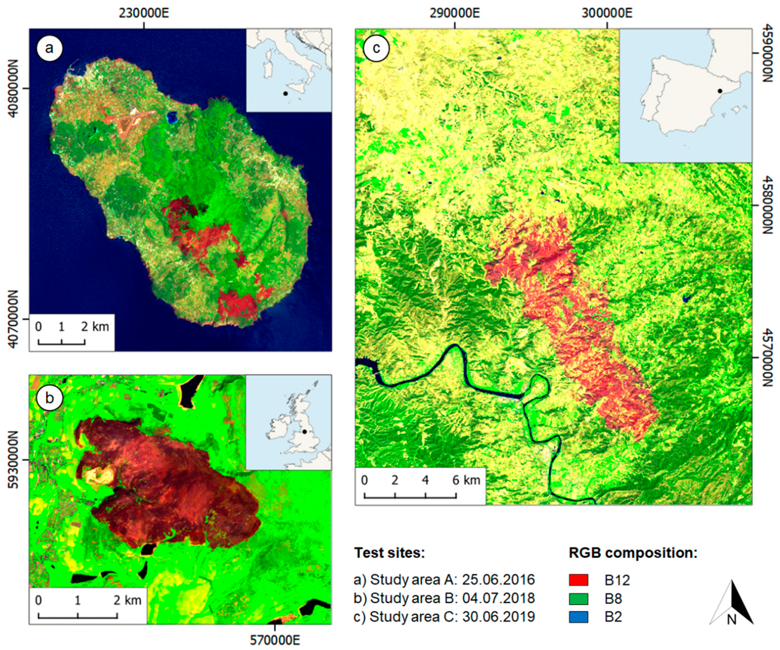
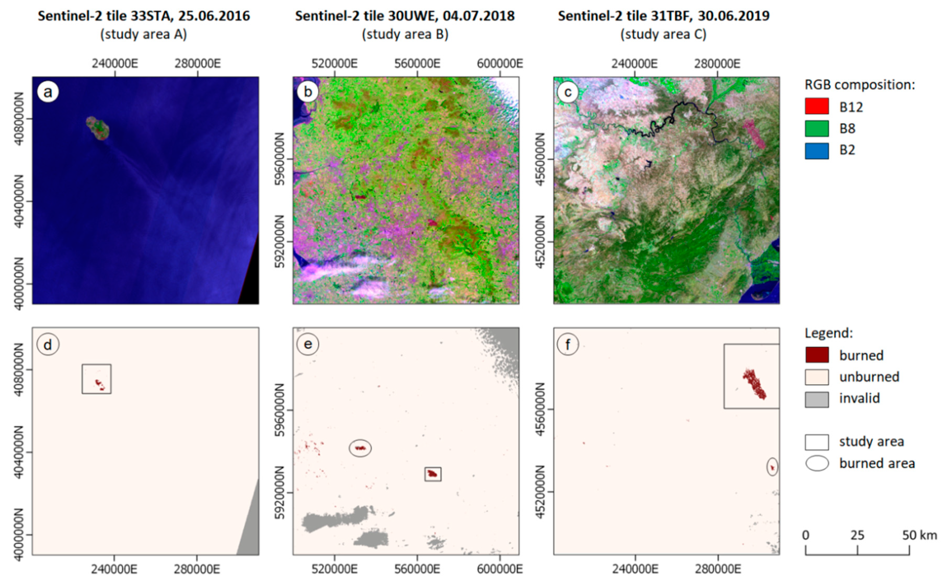
To independently test the burned area mapping module, we selected three fire events located in Pantelleria, Italy (study area A), Mossley, United Kingdom (study area B) and Torre de l’Espanyol, Spain (study area C), which were mapped as a part of Copernicus EMS. As these products have been generated in rapid mapping mode by different operators, burned area masks were manually refined to ensure high quality and to harmonize variable mapping styles. The Sentinel-2 scenes were clipped to the area of interest defined by Copernicus EMS. An overview of the three fire events can be found in Figure 2.
In June 2016, several fires broke out in the region of Sicily caused by high temperatures of up to 40 °C and strong southern winds [53]. One of the fires occurred on the island of Pantelleria (study area A) and destroyed about 600 ha of croplands, scrubs and woodlands. In response to this event, the EMS rapid mapping component was activated on June 23, 2016 (EMSR 169). Emergency maps were produced and released by e-GEOS, based on a Sentinel-2 pre-event image (10 m ground sampling distance (GSD)) acquired on April 16, 2017 and a Sentinel-2 post-event image (10 m GSD) acquired on June 25, 2016. We used the post-event Sentinel-2 image (tile 33STA) as input for testing.
In June 2018, a fire broke out in Saddleworth Moor to the east of Manchester, England (study area B) [54]. The fire affected an area of about 1000 ha, mainly characterized by inland wetlands, but also with shrub/herbaceous vegetation and pastures. In response to this event, the EMS rapid mapping component was activated on June 27, 2018 (EMSR 291). Emergency maps were produced by e-GEOS and released by SERTIT, based on a Sentinel-2 pre-event image (10 m GSD) acquired on June 24, 2018 and a SPOT-7 post-event image acquired on July 4, 2018 (1.5 m GSD). We used a Sentinel-2 scene (10 m GSD) from July 4, 2018 (tile 30UWE) for testing.
In June 2019, a wildfire broke out in the municipality of Torre de l’Espanyol in the province of Catalonia (study area C) [55]. Subsequently, nearly 5000 ha were devastated, including forests, agricultural areas and shrub/herbaceous vegetation. In response to this event, the EMS rapid mapping component was activated on June 27, 2019 (EMSR 365). Emergency maps were produced by SERTIT and released by e-GEOS based on a SPOT6/7 pre-event image (1.5 m GSD) acquired on June 6, 2019 and a SPOT-6/7 post-event image (1.5 m GSD) acquired on June 30, 2019. We used a Sentinel-2 scene (10 m GSD) from June 30, 2019 (tile 31TBF) for testing.
2.2. Fully Automatic Processing Chain
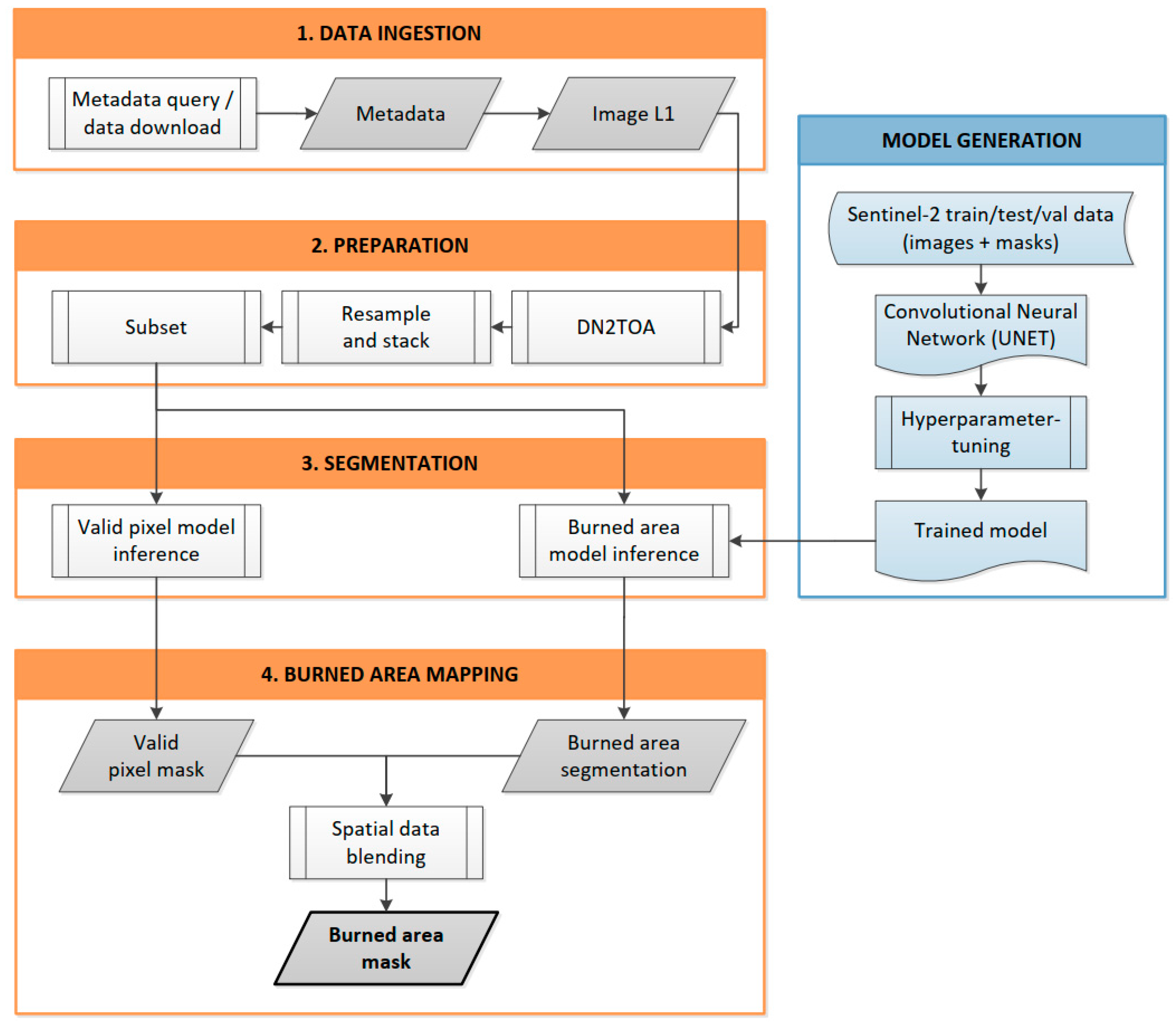
The fully automatic burned area mapping workflow is presented in Figure 3.
It is based on a modular Sentinel-2/Landsat processing chain developed at DLR, which was originally designed for flood mapping. The processing chain is fully implemented in Python using Keras with TensorFlow backend [56] as the deep learning framework. The principle components are explained in the following paragraph, for a detailed description see [43].
Two input arguments are mandatory to initiate the processing chain: an area of interest and a time range to search for satellite imagery. Optionally, further parameters can be defined such as maximum cloud coverage or the download of a quick look. The first step checks for and downloads Sentinel-2 scenes at processing level L1C that meet the defined criteria. The level L1C data product is already radiometrically calibrated and orthorectified but is not atmospherically corrected. Data can be downloaded via the ESA Copernicus Open Access Hub, using the custom Application Programming Interface (API), and is provided as single band raster files in 100 × 100 km tiles. In the following step, the downloaded data are preprocessed. Images are converted from DN to TOA reflectance (DN2TOA). The single band raster files are resampled to the same spatial resolution (10 m) and those bands required for the neural network model are stacked to produce a single dataset. In this work, the spectral bands in the following domains are used: visual (Blue, Green, Red), near infrared (NIR) and short-wave infrared (SWIR1, SWIR2). This band combination was selected for based on the outcomes of comprehensive performance evaluation described in Section 3.
The preprocessed images are passed through a first CNN to segment invalid pixels (cloud, cloud shadows, snow and ice), following the procedure described in [42], which results in a valid pixel mask. Subsequently, the same image is passed through a second CNN that has been trained specifically for a corresponding mapping task, in this case burned area segmentation. The network assigns each pixel to a corresponding class, either burned or unburned. Finally, the segmentation result is clipped to the extent of the valid pixel mask and the final burned area mask is generated.
2.3. Semantic Segmentation of Burned Areas with a U-Net CNN
The key part of this work is the development of a deep learning model based on a CNN specifically suited for burned area segmentation. A neural network is a system of interconnected neurons that is used to model a complex function, in our case, a function to map a set of pixel values to labels. A defined set of weights serves to define the function. Neurons are arranged as multiple cascading layers allowing features to be learned in a hierarchical manner. During training, input tiles are propagated through the network and a loss function is calculated to evaluate the quality of the mapping function. Gradients of the loss function are then back-propagated through the network and weights are adjusted accordingly to minimize the loss.
A critical point that affects the network’s performance is the network architecture. The architecture used in this work is based on a U-Net architecture [57]. The U-Net architecture was originally designed for biomedical image segmentation, but already achieved promising accuracies in other segmentation tasks with satellite imagery, such as cloud/cloud shadow [42] and water segmentation [43]. Further advantages of this architecture are that it can learn from a limited amount of data and has considerably less trainable parameters than other CNNs. We decided against using a pre-trained model, which is a common approach to reduce computational effort, because any new dataset would have to be similar to the one used in pre-training. This would have otherwise limited the choice of input data.
The U-Net is a fully convolutional network with encoder-decoder architecture. This means that in addition to the contracting part of a conventional CNN, the network has a more or less symmetric upsampling part. This leads to the typical u-shape of the network (see Figure 4). The U-Net presented in this work requires tiles with 6 spectral bands and a width and height of 256 pixels each. This tile size is frequently used for U-Net architectures [42,43] and has been observed to ensure that a significantly large batch size can be trained with a standard desktop PC. Images to be processed are usually larger than the specified dimension and must be tiled. We apply mirror-padding to minimize higher prediction errors towards the image border during inference and split the image into 256 × 256 pixel tiles with an overlap of 10%. These tiles are passed through the network, resulting in tiles that indicate the probability of being burned (ranging from 0 to 1).
The final binary output is calculated using a fixed threshold of 0.5. Finally, the tiles are reconstructed to the original image size. We use a tapered cosine window function w (Equation (1)) to blend the overlapping prediction tiles in which n represents the samples, N the number of pixels in the output window and α the fraction of the window inside the cosine tapered region.
In the following paragraph, the architecture of the U-Net is explained more in detail. In the encoder part, input data are passed through five convolutional blocks where features are extracted at different scales. Each convolutional block consists of two 3 × 3 convolutions with ReLu activation, each followed by batch normalization of the activations of the previous layer and ends with a max pooling operation with stride 2 that downsamples the feature maps. While the size of the feature maps is reduced by factor 4 after each convolutional block, the number of feature channels is doubled. In the decoder part, the feature maps are upsampled to the original image size by passing through five blocks as well. Each of these blocks consists of a 2 × 2 transpose convolution that halves the number of feature channels, a concatenation with the corresponding feature map from the encoder part and two 3 × 3 convolutions with ReLu activation, each followed by batch normalization. The final layer is a 1 × 1 convolution with sigmoid activation in order to calculate the probability for each pixel of being burned.
2.4. Training of the U-Net CNN
To define the weights of the U-Net, the network was trained on the augmented dataset presented in Section 2.1. Augmentation was applied in order to make the network invariant to specific transformations: the geometric transformations simulate different sensor characteristics such as spatial resolution. Thus, the network could potentially be used to process image data from other satellite sensors (e.g., Landsat). The radiometric transformations aim to capture variations with seasonality, land use, land cover and under different atmospheric conditions. The last point is especially important, as image data are not atmospherically corrected before entering the U-Net. To make the samples of the augmented dataset more comparable, all data values were standardized using the statistics of the training samples. Standardization was performed independently on each spectral band and included data-centering by subtraction of the mean and scaling to unit variance by division by the standard deviation.
During training, weights were adjusted after each epoch in a way that minimized the binary cross entropy loss H of the training data, between the true probability p and the predicted probability Equation (2). Training data were shuffled after each epoch.
We used the adaptive moment estimation (Adam) optimization algorithm [58] with an initial learning rate of 0.001 and default hyper-parameters β1 = 0.9 and β2 = 0.999. Validation data were also passed through the network during training and its loss was calculated and monitored. If validation loss did not improve within five epochs, the learning rate was reduced by factor 0.5. To prevent overfitting, training was stopped if validation loss has not improved within 20 epochs. At the end of the training process, the model associated with the lowest validation loss was saved. Training was carried out on a standard desktop PC with Intel XEON W-2133 CPU @ 3.60 GHz, 6 cores, 64 GB RAM and NVIDIA Quadro P4000 graphic card. The network was trained until convergence occurred in batches of size 16, using Keras with TensorFlow backend [56] as the deep learning framework.
2.5. Accuracy Assessment
For model evaluation, we forwarded the testing data through the network and calculated overall accuracy, Cohen’s kappa coefficient, inference speed as well as precision and recall of the pixels classified as burned. Overall, accuracy OA is defined as the number of correctly classified pixels over the total number of pixels, see Equation (3) (tp = true positive, tn = true negative, fp = false positive, fn = false negative). Cohens’ kappa coefficient K is an indicator of interrater reliability and is calculated with Equation (4). The variable p0 describes the observed overall accuracy and pe is the expected probability, when both raters assign labels randomly.
As overall accuracy is mainly influenced by the quantity of unburned pixels due to the unbalanced distribution of classes, we also calculated precision and recall of the burned class, which are also referred to as user’s accuracy and producer’s accuracy. Precision describes how many detected burned pixels are in fact burned Equation (5), whereas recall describes how many of the truly burned pixels have been detected as such Equation (6). Additionally, we calculated the F1 score, which is the mean of precision and recall.
We additionally trained a random forest model for benchmarking. We used the Scikit-learn implementation [59] with standard parameters, which fits a number of optimized CART decision trees [60] on subsamples of the training data and uses averaging to prevent overfitting and to improve the accuracy of the prediction.
To test the complete processing chain and to evaluate the performance of our network model in real-world emergency response applications, we processed the Sentinel-2 scenes of the study areas A–C and compared the results to the reference data.
3. Results
In order to find an optimal input data configuration for the CNN, we tested different band combinations before training a final network. The objective was to achieve best results with as few spectral bands as possible. This approach makes the model lighter, reduces inference and processing time and minimizes storage space requirements. Table 2 gives an overview of the spectral band combinations tested, starting with a combination of all spectral bands (BC1) and then gradually reducing the number of bands. First, we removed all atmospheric bands (BC2), then the narrow bands of the red edge domain (BC3). Afterwards, we omitted the bands of the SWIR domain (BC4) and finally trained a network with the spectral bands of the visual domain only (BC5). All networks were trained on the non-augmented dataset until convergence occurred. Inference time was averaged over five runs and refers to a calculation on the graphics processing unit (GPU).
Table 2 shows that the accuracy assessment for BC1–BC4 varies only slightly. Changes cannot be clearly traced back to different band combinations, as they could also be based on different randomly set initial weights. Nevertheless, accuracy and kappa show a downward trend with lower numbers of spectral bands used for training. Training the network exclusively with the blue, green and red channels clearly results in worse outcomes. In the end, we selected BC3, a tradeoff between high accuracy and low inference time with balanced outcomes for precision and recall. Furthermore, this band combination can also be found in other multispectral satellite sensors, such as Landsat, which allows testing the transferability of the Sentinel-2 trained model to other sensor data.
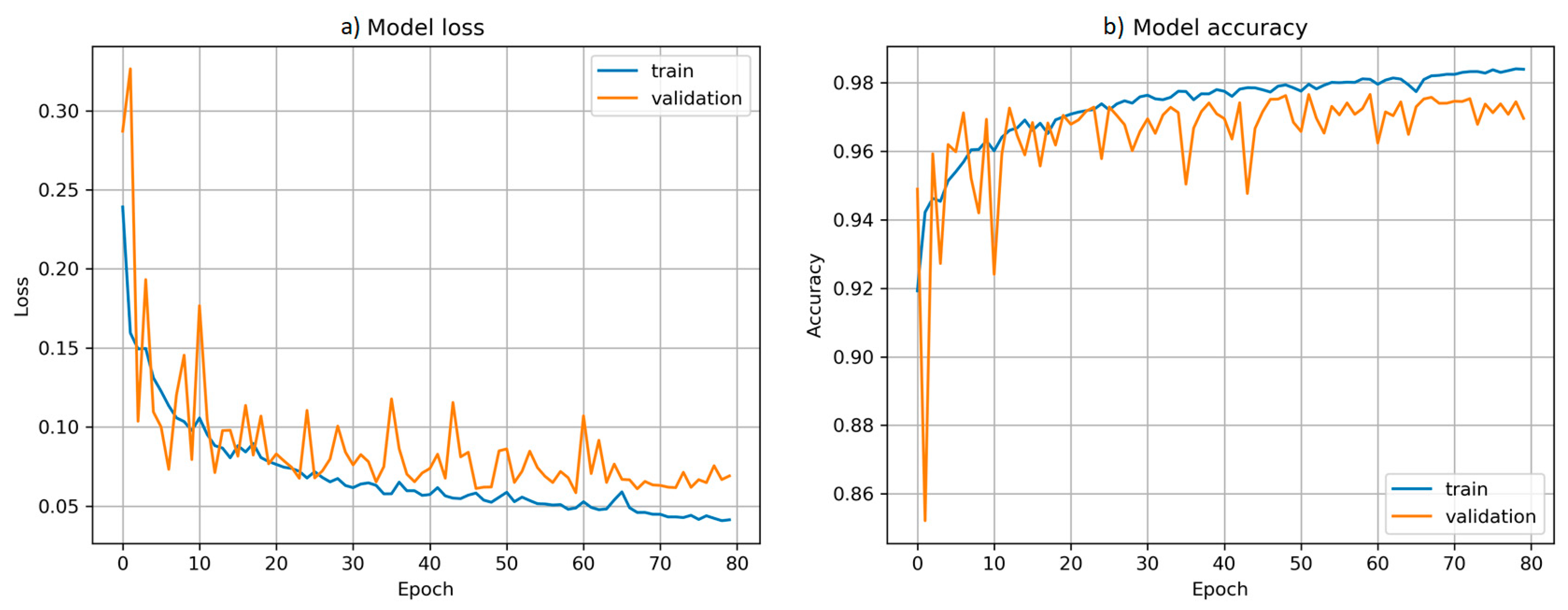
The final model was trained on the augmented dataset using the spectral bands of BC3. Training lasted about 4 hours using the hardware described in Section 2.4. Figure 5 shows the loss and accuracy of the training and validation datasets over the epochs.
The results of the accuracy assessment for the testing tiles are summarized in Table 3. For the U-Net model, we achieved an overall accuracy of 0.98 and a precision and a recall of the burned class of 0.95 each. The central processing unit (CPU) inference speed computed over 545 test image tiles is 2.20 s/megapixel and the corresponding GPU inference speed is 0.26 s/megapixel. Compared to the RF model, the U-Net model resulted in significantly better metrics: overall accuracy is 0.02 higher and the kappa coefficient is 0.07 higher. In particular, the inference time of the RF model is almost twice as long. Calculating on the GPU even makes the U-Net 15 times faster.
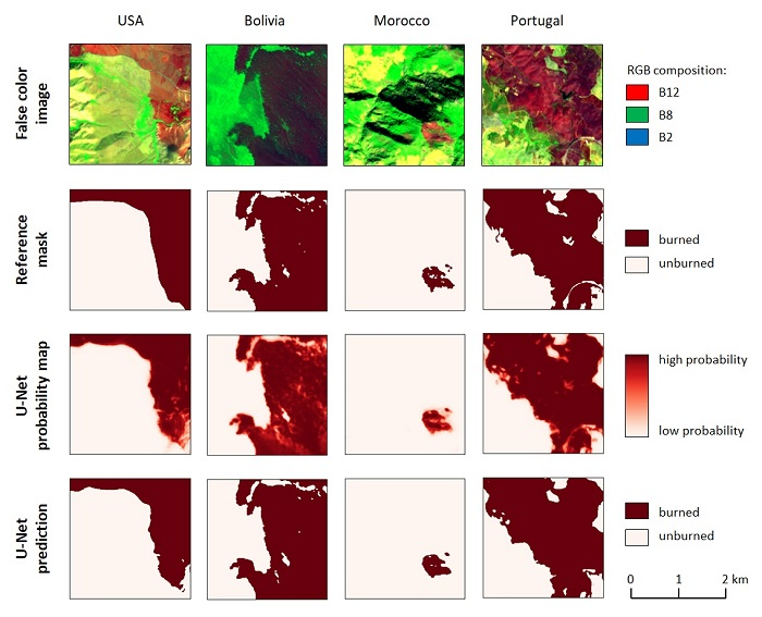
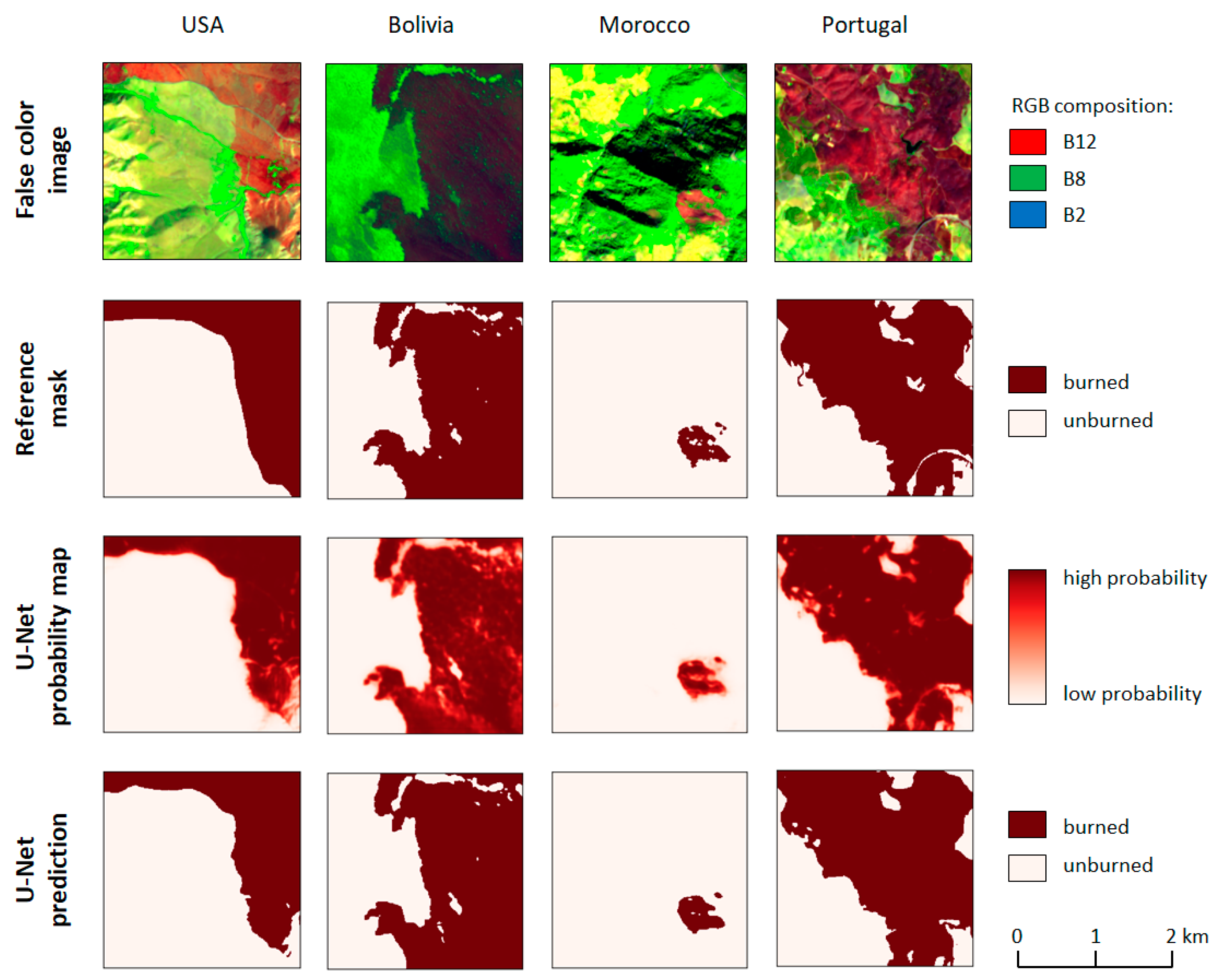
Figure 6 exemplifies the results for four testing tiles originating from different countries. A composition of the B12, B8 and B2 spectral bands is displayed, as well as the respective reference mask, U-Net probability map and U-Net prediction. The burned area delineations of the U-Net are precise and, in the case based in the USA, reflect actual conditions even better than the reference mask. This also emphasizes the difference between the CAL FIRE and ICNF data (examples of homogenous burned area extent for the USA and Portugal) and the DLR data (examples of pixelwise segmentation for Bolivia and Morocco) as described in Section 2.1 and Section 5.
To test the complete processing chain, we processed the Sentinel-2 scenes that include study areas A–C. After downloading the scenes, the average processing time for data preparation, segmentation and final mapping was 193 s. Figure 7 shows the corresponding results and supports an initial qualitative analysis. Clouds, cloud shadows and no data values (e.g., in Figure 7a) are identified and classified as invalid pixels. The burned areas of study sites A–C are detected, as well the two other burned areas that are present in tiles 30UWE and 31TBF. These areas are indicated with circles. In general, there are only limited instances of false detections. In tile 31TBF, open-cast mining is frequently incorrectly identified as burned area, while in tile 30UWE, false detections mainly occur over agricultural fields, especially in the left side of Figure 7e.
To avoid an over-representation of background pixels within the full Sentinel-2 scenes in our accuracy metrics, we focus on study areas A–C for a more detailed accuracy assessment. Table 4 presents the quantitative results associated with the three study areas. The overall accuracy is 99% in all three cases, while kappa varies between 86% and 97%. The precision of the predicted burned pixels shows the largest variability: while it is just 77% in study area A, it is 96% in study area B. In contrast, the recall of the burned class is consistently high at an average of 0.98% and differs only marginally in the three cases.
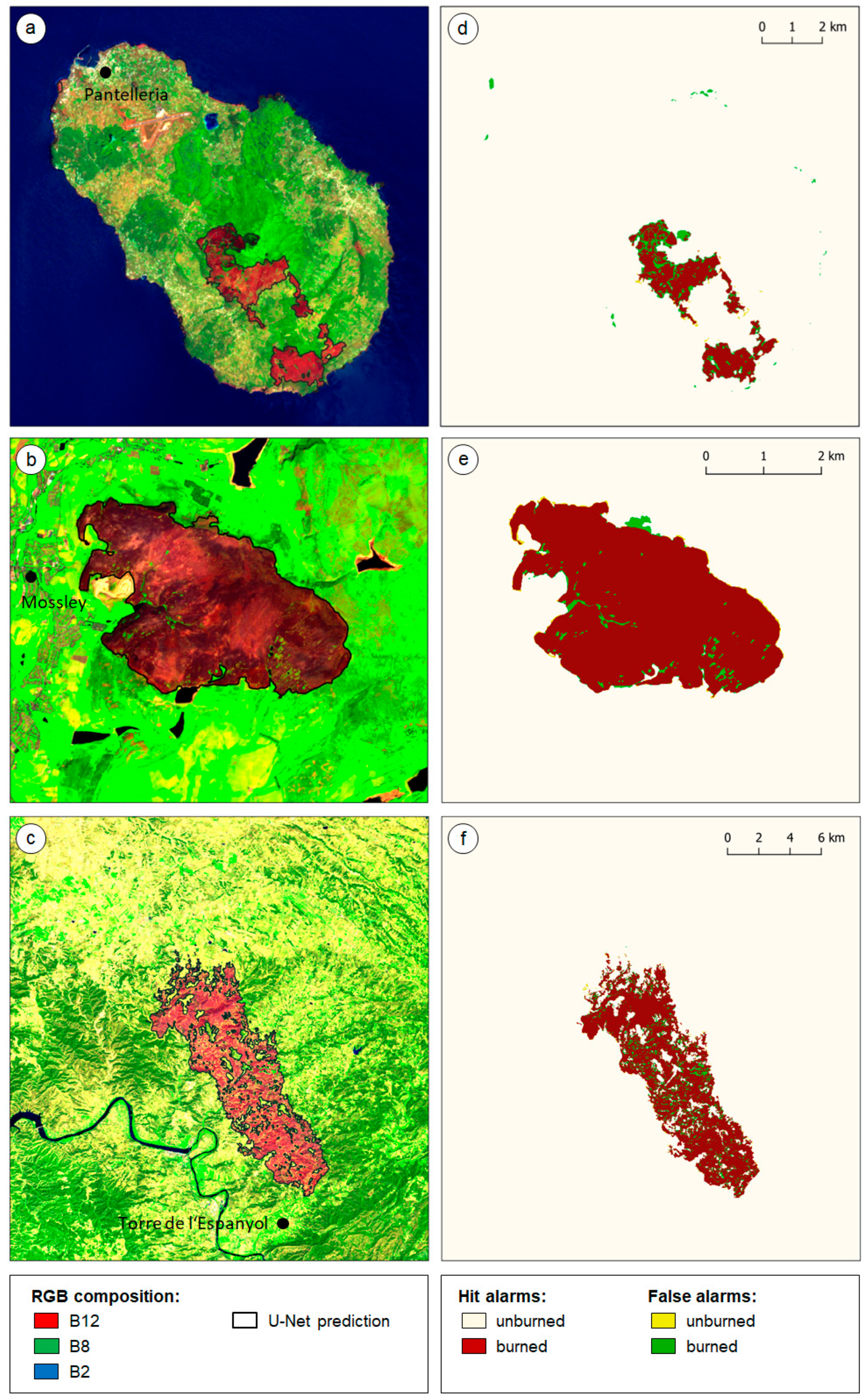
For a qualitative accuracy assessment, we visualized the U-Net prediction on an image composite with B12, B8 and B2 spectral bands and identified hit and false alarms (see Figure 8). Misclassifications mainly occur within or directly connected to the burned areas. Only in case of study area A there are also false burned alarms in the coastal area of the island. Thin structures, such as roads, are usually not detected as unburned. In general, false alarms in the predicted burned class clearly outweigh those in the unburned class.
4. Discussion
One of the most important aspects that can influence the performance of any supervised machine learning algorithm is the choice of appropriate training data. Thus, in the first part of the discussion, we review the impact of several choices we made on the network’s performance.
As described in Section 2.1, we did not only use those tiles for training that included both classes (burned and unburned), but also tiles completely covered by one class. This enables the network to learn more about unburned areas such as harvested cropland, which had caused major problems in other segmentation approaches [17]. To show the impact of this single class tile integration, we trained an additional network excluding these tiles and processed the Sentinel-2 data of the three study areas in Italy (A), UK (B) and Spain (C). Figure 9 presents the respective probability maps.
The probability maps resulting from both models generally show segmentation difficulties in the same areas: the rocky coastline in study area A and the lakeshore in the east and agricultural fields in the north of the burned area in study area B. However, as can be seen in Figure 9e, the model trained without single class tiles assigns a lot higher probability of being burned to those misclassifications. Furthermore, not integrating single class tiles results in further misclassifications such as predicting the airport site in study area A as burned. These findings justify our decision to integrate single class tiles in the training dataset for our final network model.
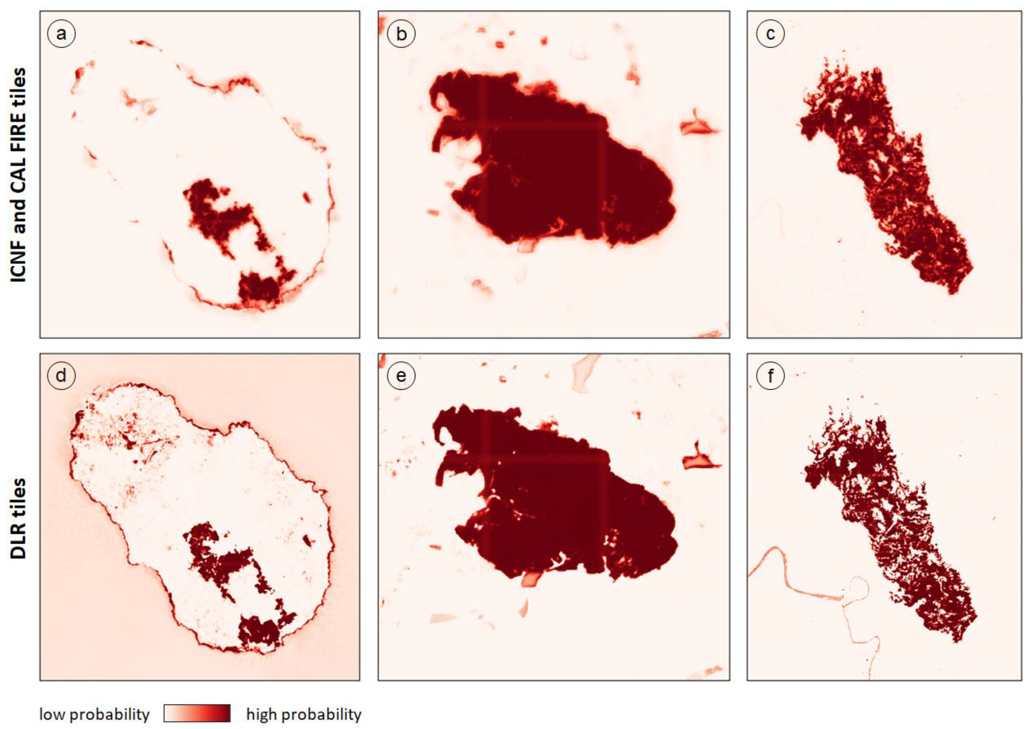
Besides the integration of single class tiles, the kind of reference data used for training also has influence on the network’s results. In this work, we included pixelwise burned area masks produced by a DLR processor [17] and burned area perimeters of ICNF and CAL FIRE. As previously described, the latter are characterized as the outermost extent of burned areas, rather than a more detailed pixel-by-pixel segmentation. To show the impact on the network’s performance, we trained two additional networks: the first one using only the pixelwise burned area masks of DLR (798 tiles) and the second one using the areal burned area masks of ICNF and CAL FIRE (3906 tiles). Figure 10 presents the resulting probability maps. It is noticeable that the model trained with DLR tiles only results in a sharp delineation of the burned areas from their surroundings, while the model trained with ICNF and CAL FIRE data produces gradually decreasing probabilities at the borders of the burned areas. Furthermore, misclassifications occur more frequently and more clearly in the model trained with DLR data only. This is probably due to the fact that ICNF and CALFIRE provide their data as vector files representing the extent of the burned area, rather than a per pixel segmentation. The network learns this characteristic and takes the neighborhood much more into account to create homogenous burned areas. A further aspect that can be observed in Figure 10 is that the model trained with DLR data only is very prone to detecting water surfaces as burned areas, such as the ocean around the island in study area A, lakes in study area B and the river in study area C. Training a neural network with both datasets, as with the final model, constitutes a compromise between the advantages and disadvantages of the datasets. The corresponding probability maps are illustrated in Figure 9a–c. While there are hardly any misclassifications in water areas, however, burned areas do not have a sharp outline.
This extensive discussion of the influence of the input data on the network’s performance highlights the importance of high quality training data since the neural network always learns by imitation. Consequently, misclassifications in the inputs will be reproduced. Thus, the neural network should be ideally trained with a large amount of manually digitized burned areas and not with automatically derived products that are subject to a high degree of uncertainty. The training data used in this work do not fully meet these requirements. Nevertheless, we still achieve very good results in our final network model, even training with a freely available or automatically derived dataset without further modifications.
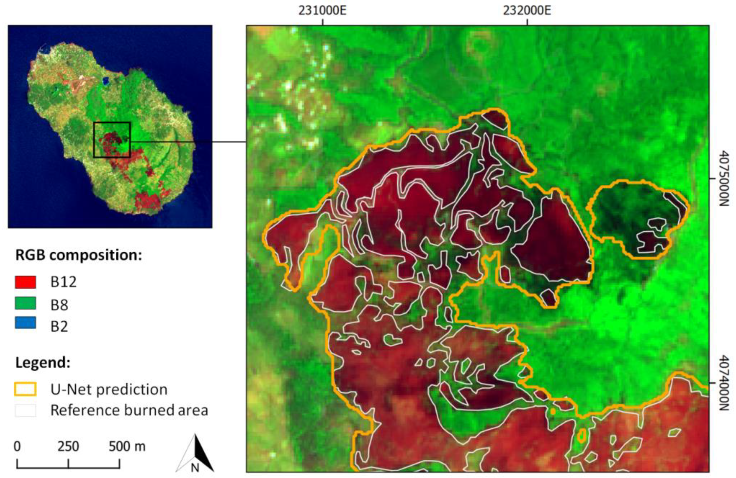
After discussing the impact of input data on the network’s results, we now focus on the segmentation results of the final network model. In Section 3, we already mentioned that major misclassifications occur at the rocky coastline of the volcanic island of Pantelleria in study area A. In previous assessments of other fire events, we also observed misclassifications of rocks of volcanic origin as burned areas. Furthermore, the probability map of study area B (Figure 9b) points to a likelihood of confusion with dark water areas and agricultural fields. However, a far greater proportion of overclassification lies within the burned areas themselves. In most instances, these are characteristically narrow areas such as roads. An explanation may be that only four of the spectral bands received by the network as input have an original spatial resolution of 10 m. The two SWIR bands only have an original resolution of 20 m, which makes it difficult to detect structures with a smaller width. However, in study area A, even islands of unaffected forest of up to four ha were included into the burned area segmentation result of the U-Net. This can be attributed to the large proportion of ICNF and CAL FIRE data within the training tiles (79%). As learned from these data, the network aims at creating homogenous burned areas even under circumstances where there are smaller unburned areas therein. Figure 11 shows an example of this observation with an inset over a burned area in study area A.
Compared to the reference burned area, which had been manually digitized based on Copernicus EMS rapid mapping products, the U-Net returns a coarse extent of the burned area rather than a pixel-based segmentation. Furthermore, the U-Net not only considers completely burned areas, but also those only partially affected, for example, the coniferous forest area located in the east of the inset. The forest here appears in a significantly darker green than in the surrounding areas. This is probably due to the fact that the forest was also affected by the fire, but the tree crowns did not burn completely. Another example of areas that are only partially affected, but still have been predicted as burned by the U-Net can be found in the central part of the inset in Figure 11. Pixels appear in light red color and change frequently to green pixels. This indicates mixed pixels, which contain both burned and unburned areas within the 100 m2 area that each pixel covers. Even when performing a visual interpretation of these two examples, it is difficult to determine whether the pixel should belong to either the burned or unburned class. This unclear definition is a general problem in burned area segmentation in earth observation data and not only refers to partially affected areas. Old burned areas are another problem. In particular, the degree to which a previously burned area has recovered needs to be defined so that under this set of conditions, such an area would no longer be considered a part of the burned class. It must be defined beforehand whether a segmentation model should be applied to only recently burned areas or also to older ones. When refining the Copernicus EMS rapid mapping products, we decided to consider only freshly burned areas that are completely destroyed. However, our training dataset contains tiles of different databases, which in turn (except for DLR data), are a collection of mapping products from different providers, each of which may have a different definition of a burned area. Therefore, the misclassifications in our three study sites are not only due to the performance of the network, but above all due to the unclear definition of burned areas. This is attributed to the network’s reception of heterogeneous training data from the three different sources and, therefore, it is unable to learn clear rules.
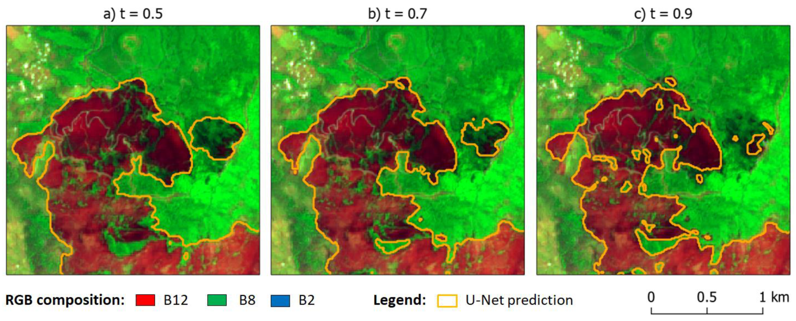
An advantageous aspect of our approach addresses this problem. In particular, the operator can decide whether to receive a segmentation of the clearly burned areas or an extent of possibly damaged areas. This is done by changing the probability threshold to predict a pixel as burned. The default threshold is set to 0.5. While increasing the threshold results in a more precise delineation of the burned area, it can also lead to the omission of partially affected areas. The operator can choose a threshold that best fits the desired mapping style and that achieves optimal results with respect to the data. Figure 12 illustrates the results based on the application of different thresholds over the same aforementioned inset in study area A.
In addition to this flexibility in defining what should be detected as burned, our approach has several other benefits. Compared to other burned area segmentation algorithms, a major advantage is that no previous feature engineering needs to be performed. This is generally not the case in RF approaches, for example. The network does not require any auxiliary data and receives as input Sentinel-2 data at level L1C, which have not been atmospherically corrected. The omission of this step significantly reduces the satellite data preprocessing time. Additionally, the overall processing time is shortened by the fact that only a post-event image is required. Compared to bi-/multi-temporal approaches, such as the one pursued so far by DLR [17] or the authors of [18], the final segmentation is less influenced by clouds because the invalid pixel mask is not composed of clouds from both a pre- and a post-fire scene. Pinto et al. [46] solved the problem attributed to the presence of clouds by using a time–series of satellite data. However, a large amount of data would have to be downloaded or be permanently provided to use this method in a rapid mapping context, for example, to provide timely burned area extents for an initial damage assessment. In contrast, our approach presents a simple and rapid end-to-end solution that includes data ingestion, preprocessing and burned area segmentation targeted towards operational use in forest fire management. For instance, the approach could be used to continuously monitor a specific region of interest. Furthermore, the use of high resolution Sentinel-2 data in our approach clearly improves the temporal availability and resolution of burned area delineations compared to methods based on Landsat or MODIS data.
The testing of our final segmentation model shows an overall accuracy of 0.98 and a kappa coefficient of 0.94. However, the three use cases show that there are still problems with misclassifications. In the future, segmentation results could be further improved by integrating additional modules to the processing workflow. As it is common in burned area mapping, the segmentation results of the U-Net could be used to determine pixels having a high probability of being burned. In a second phase, region growing could be performed to define the final burned area mask. Furthermore, areas in which fires do not occur (such as water bodies) could be masked out in advance to reduce instances of misclassifications.
While the results of this work are promising, it should be noted that our segmentation approach has only been tested on burned areas without active fires and that were not covered by clouds. However, cloud cover is a major issue, especially in tropical areas. To address this topic, the model should be tested with other optical data sources, such as Landsat and adjusted if necessary. Integration of radar data should also be considered. Furthermore, especially for long lasting fires like the Australian bush fires of 2019/20, it is likely that smoke partially covers the satellite scenes, which may impede accurate burned area mapping and, thus, needs to be specifically addressed.
To date, we performed an extensive validation of our model on three selected fire events. However, as the qualitative analysis of the corresponding Sentinel-2 scenes has shown, there are specific areas that are prone to be falsely detected as burned areas, such as agricultural fields or open-cast mining areas. In the future, the model will be tested over larger regions to identify any additional, problematic area. Furthermore, we expect to improve our training data so that all biomes prone to fire events are fully represented, to realize the long-term goal of developing a model for global application.
5. Conclusions
In this work, we aimed at combining sensor and method developments of the past few years. We proposed a fully automatic processing chain to segment burned areas in Sentinel-2 imagery, including data ingestion, data preprocessing and burned area mapping. Hence, rapid mapping agencies tasked with burned area mapping could apply the methodology without having to manually download and preprocess data and can, thus, benefit from the available high-resolution Sentinel-2 data. Our segmentation model is based on a deep neural network and achieves an overall accuracy of 0.98 and kappa coefficient of 0.94. However, as our independent tests have shown, there are still some problems with certain types of misclassifications, especially at the shores of dark water bodies, in agricultural fields and for rocks of volcanic origin. Furthermore, our model tends to create a homogenous burned area mask closing small unaffected areas. However, the operator can counteract this by raising the probability threshold to detect a pixel as burned. To verify the global applicability of our model, further testing must be conducted, especially over a more comprehensive range of biomes. Furthermore, to ensure the utility of the model during ongoing fire events, the proposed processing chain should be extended with the inclusion of a smoke detection module.
Author Contributions
Conceptualization, L.K., M.W., M.R. and S.M.; methodology, L.K. and M.W.; software, L.K. and M.W.; validation, L.K.; formal analysis, L.K.; investigation, L.K.; data curation, L.K. and M.R.; writing—original draft preparation, L.K.; writing—review and editing, L.K., M.W. and S.M.; visualization, L.K.; supervision, M.W., M.R. and S.M. All authors have read and agreed to the published version of the manuscript.
Funding
This research received no external funding.
Acknowledgments
The authors would like to thank the editors and the anonymous reviewers for their constructive comments and suggestions that helped to improve this manuscript, as well as Candace Chow for the language editing.
Conflicts of Interest
The authors declare no conflicts of interest. The funders had no role in the design of the study; in the collection, analyses or interpretation of data; in the writing of the manuscript or in the decision to publish the results.
References
- Kelly, L.T.; Brotons, L. Using fire to promote biodiversity. Science 2017, 355, 1264–1265. [Google Scholar] [CrossRef] [PubMed]
- Chuvieco, E.; Mouillot, F.; van der Werf, G.R.; San Miguel, J.; Tanase, M.; Koutsias, N.; García, M.; Yebra, M.; Padilla, M.; Gitas, I.; et al. Historical background and current developments for mapping burned area from satellite Earth observation. Remote Sens. Environ. 2019, 225, 45–64. [Google Scholar] [CrossRef]
- Bowman, D.M.J.S.; Balch, J.K.; Artaxo, P.; Bond, W.J.; Carlson, J.M.; Cochrane, M.A.; D’Antonio, C.M.; DeFries, R.S.; Doyle, J.C.; Harrison, S.P.; et al. Fire in the Earth system. Science 2009, 324, 481–484. [Google Scholar] [CrossRef]
- Lewis, S.L.; Edwards, D.P.; Galbraith, D. Increasing human dominance of tropical forests. Science 2015, 349, 827–832. [Google Scholar] [CrossRef]
- Thonicke, K.; Spessa, A.; Prentice, I.C.; Harrison, S.P.; Dong, L.; Carmona-Moreno, C. The influence of vegetation, fire spread and fire behaviour on biomass burning and trace gas emissions: Results from a process-based model. Biogeosciences 2010, 7, 1991–2011. [Google Scholar] [CrossRef] [Green Version]
- Yue, C.; Ciais, P.; Cadule, P.; Thonicke, K.; Van Leeuwen, T.T. Modelling the role of fires in the terrestrial carbon balance by incorporating SPITFIRE into the global vegetation model ORCHIDEE—Part 2: Carbon emissions and the role of fires in the global carbon balance. Geosci. Model Dev. 2015, 8, 1321–1338. [Google Scholar] [CrossRef] [Green Version]
- Chuvieco, E.; Aguado, I.; Yebra, M.; Nieto, H.; Salas, J.; Martín, M.P.; Vilar, L.; Martinez, J.; Martín, S.; Ibarra, P.; et al. Development of a framework for fire risk assessment using remote sensing and geographic information system technologies. Ecol. Model. 2010, 221, 46–58. [Google Scholar] [CrossRef]
- Global Assessment Report on Disaster Risk Reduction 2019. Available online: https://gar.undrr.org/sites/default/files/reports/2019-05/full_gar_report.pdf (accessed on 7 January 2020).
- Nolde, M.; Plank, S.; Riedlinger, T. An Adaptive and Extensible System for Satellite-Based, Large Scale Burnt Area Monitoring in Near-Real Time. Remote Sens. 2020, 12, 2162. [Google Scholar] [CrossRef]
- Laris, P.S. Spatiotemporal problems with detecting and mapping mosaic fire regimes with coarse-resolution satellite data in savanna environments. Remote Sens. Environ. 2005, 99, 412–424. [Google Scholar] [CrossRef]
- Roy, D.P.; Jin, Y.; Lewis, P.E.; Justice, C.O. Prototyping a global algorithm for systematic fire-affected area mapping using MODIS time series data. Remote Sens. Environ. 2005, 97, 137–162. [Google Scholar] [CrossRef]
- Chuvieco, E.; Lizundia-Loiola, J.; Pettinari, M.L.; Ramo, R.; Padilla, M.; Tansey, K.; Mouillot, F.; Laurent, P.; Storm, T.; Heil, A.; et al. Generation and analysis of a global burned area product based on MODIS 250m reflectance bands and thermal anomalies. Earth Syst. Sci. Data 2018, 512, 1–24. [Google Scholar] [CrossRef]
- Giglio, L.; Boschetti, L.; Roy, D.P.; Humber, M.L.; Justice, C.O. The Collection 6 MODIS burned area mapping algorithm and product. Remote Sens. Environ. 2018, 217, 72–85. [Google Scholar] [CrossRef] [PubMed]
- San-Miguel-Ayanz, J.; Schulte, E.; Schmuck, G.; Camia, A.; Strobl, P.; Liberta, G.; Giovando, C.; Boca, R.; Sedano, F.; Kempeneers, P.; et al. Comprehensive monitoring of wildfires in Europe: The European forest fire information system (EFFIS). In Approaches to Managing Disasters—Assessing Hazards, Emergencies and Disaster Impacts; Tiefenbacher, J., Ed.; IntechOpen: Rijeka, Croatia, 2012; pp. 87–108. [Google Scholar]
- Hawbaker, T.J.; Vanderhoof, M.K.; Beal, Y.-J.; Takacs, J.D.; Schmidt, G.L.; Falgout, J.F.; Williams, B.W.; Fairaux, N.M.; Caldwell, M.K.; Picotte, J.J.; et al. Mapping burned areas using dense time-series of Landsat data. Remote Sens. Environ. 2017, 198, 504–522. [Google Scholar] [CrossRef]
- Stavrakoudis, D.G.; Katagis, T.; Minakou, C.; Gitas, I.Z. Towards a fully automatic processing chain for operationally mapping burned areas countrywide exploiting Sentinel-2 imagery. In Proceedings of the Seventh International Conference on Remote Sensing and Geoinformation of the Environment (RSCy2019), Paphos, Cyprus, 18–21 March 2019; p. 1117405. [Google Scholar]
- Bettinger, M.; Martinis, S.; Plank, S. An Automatic Process Chain for Detecting Burn Scars Using Sentinel-2 Data. In Proceedings of the 11th EARSeL Forest Fires SIG Workshop, Chania, Greece, 25–27 September 2017. [Google Scholar]
- Pulvirenti, L.; Squicciarino, G.; Fiori, E.; Fiorucci, P.; Ferraris, L.; Negro, D.; Gollini, A.; Severino, M.; Puca, S. An Automatic Processing Chain for Near Real-Time Mapping of Burned Forest Areas Using Sentinel-2 Data. Remote Sens. 2020, 12, 674. [Google Scholar] [CrossRef] [Green Version]
- Roteta, E.; Bastarrika, A.; Padilla, M.; Storm, T.; Chuvieco, E. Development of a Sentinel-2 burned area algorithm: Generation of a small fire database for sub-Saharan Africa. Remote Sens. Environ. 2018, 222, 1–17. [Google Scholar] [CrossRef]
- Navarro, G.; Caballero, I.; Silva, G.; Parra, P.C.; Vázquez, Á.; Caldeira, R. Evaluation of forest fire on Madeira Island using Sentinel-2A MSI imagery. Int. J. Appl. Earth Obs. Geoinf. 2017, 58, 97–106. [Google Scholar] [CrossRef] [Green Version]
- Lasaponara, R.; Tucci, B.; Ghermandi, L. On the use of satellite Sentinel 2 data for automatic mapping of burnt areas and burn severity. Sustainability 2018, 10, 3889. [Google Scholar] [CrossRef] [Green Version]
- Filipponi, F. Exploitation of Sentinel-2 Time Series to Map Burned Areas at the National Level: A Case Study on the 2017 Italy Wildfires. Remote Sens. 2019, 11, 622. [Google Scholar] [CrossRef] [Green Version]
- Fernández-Manso, A.; Fernández-Manso, O.; Quintano, C. SENTINEL-2A red-edge spectral indices suitability for discriminating burn severity. Int. J. Appl. Earth Obs. Geoinf. 2016, 50, 170–175. [Google Scholar] [CrossRef]
- CAL FIRE Incidents Overview. Available online: https://www.fire.ca.gov/incidents (accessed on 1 September 2019).
- Cartografía de area ardida. Available online: http://www2.icnf.pt/portal/florestas/dfci/inc/mapas (accessed on 1 September 2019).
- Key, C.H.; Benson, N.C. Measuring and remote sensing of burn severity: The CBI and NBR. In Proceedings of the Joint Fire Science Conference and Workshop, Boise, ID, USA, 15–17 June 1999; Volume 2000, pp. 284–285. [Google Scholar]
- Trigg, S.; Flasse, S. An evaluation of different bi-spectral spaces for discriminating burned shrub-savannah. Int. J. Remote Sens. 2001, 22, 2641–2647. [Google Scholar] [CrossRef]
- Martín, M.P.; Gómez, I.; Chuvieco, E. Performance of a burned-area index (BAIM) for mapping Mediterranean burned scars from MODIS data. In Proceedings of the 5th International Workshop on Remote Sensing and GIS Applications to forest fire management: Fire effects assessment, Zaragoza, Spain, 16–18 June 2005; pp. 193–198. [Google Scholar]
- Ramo, R.; Chuvieco, E. Developing a Random Forest algorithm for MODIS global burned area classification. Remote Sens. 2017, 9, 1193. [Google Scholar] [CrossRef] [Green Version]
- Roy, D.P.; Huang, H.; Boschetti, L.; Giglio, L.; Yan, L.; Zhang, H.H.; Li, Z. Landsat-8 and Sentinel-2 burned area mapping—A combined sensor multi-temporal change detection approach. Remote Sens. Environ. 2019, 231, 111254. [Google Scholar] [CrossRef]
- Petropoulos, G.P.; Kontoes, C.; Keramitsoglou, I. Burnt area delineation from a uni-temporal perspective based on Landsat TM imagery classification using support vector machines. Int. J. Appl. Earth Obs. Geoinf. 2011, 13, 70–80. [Google Scholar] [CrossRef]
- Zhang, R.; Qu, J.J.; Liu, Y.; Hao, X.; Huang, C.; Zhan, X. Detection of burned areas from mega-fires using daily and historical MODIS surface reflectance. Int. J. Remote Sens. 2015, 36, 1167–1187. [Google Scholar] [CrossRef]
- Al-Rawi, K.R.; Casanova, J.L.; Calle, A. Burned area mapping system and fire detection system, based on neural networks and NOAA-AVHRR imagery. Int. J. Remote Sens. 2015, 22, 2015–2032. [Google Scholar] [CrossRef]
- Brivio, P.A.; Maggi, M.; Binaghi, E.; Gallo, I. Mapping burned surfaces in Sub-Saharan Africa based on multi-temporal neural classification. Int. J. Remote Sens. 2003, 24, 4003–4016. [Google Scholar] [CrossRef]
- Gimeno, M.; San-Miguel-Ayanz, J. Evaluation of RADARSAT-1 data for identification of burnt areas in Southern Europe. Remote Sens. Environ. 2004, 92, 370–375. [Google Scholar] [CrossRef]
- Petropoulos, G.P.; Vadrevu, K.P.; Xanthopoulos, G.; Karantounias, G.; Scholze, M. A comparison of spectral angle mapper and artificial neural network classifiers combined with Landsat TM imagery analysis for obtaining burnt area mapping. Sensors 2010, 10, 1967–1985. [Google Scholar] [CrossRef] [Green Version]
- Gómez, I.; Martín, M.P. Prototyping an artificial neural network for burned area mapping on a regional scale in Mediterranean areas using MODIS images. Int. J. Appl. Earth Obs. Geoinf. 2011, 13, 741–752. [Google Scholar] [CrossRef]
- Ramo, R.; García, M.; Rodríguez, D.; Chuvieco, E. A data mining approach for global burned area mapping. Int. J. Appl. Earth Obs. Geoinf. 2018, 73, 39–51. [Google Scholar] [CrossRef]
- Ba, R.; Song, W.; Li, X.; Xie, Z.; Lo, S. Integration of multiple spectral indices and a neural network for burned area mapping based on MODIS data. Remote Sens. 2019, 11, 326. [Google Scholar] [CrossRef] [Green Version]
- Maggiori, E.; Tarabalka, Y.; Charpiat, G.; Alliez, P. Convolutional neural networks for large-scale remote-sensing image classification. IEEE Trans. Geosci. Remote Sens. 2016, 55, 645–657. [Google Scholar] [CrossRef] [Green Version]
- Wurm, M.; Stark, T.; Zhu, X.X.; Weigand, M.; Taubenböck, H. Semantic segmentation of slums in satellite images using transfer learning on fully convolutional neural networks. Isprs J. Photogramm. Remote Sens. 2019, 150, 59–69. [Google Scholar] [CrossRef]
- Wieland, M.; Li, Y.; Martinis, S. Multi-sensor cloud and cloud shadow segmentation with a convolutional neural network. Remote Sens. Environ. 2019, 230, 1–22. [Google Scholar] [CrossRef]
- Wieland, M.; Martinis, S. A modular processing chain for automated flood monitoring from multi-spectral satellite data. Remote Sens. 2019, 11, 2330. [Google Scholar] [CrossRef] [Green Version]
- Luus, F.P.S.; Salmon, B.P.; den Bergh, F.; Maharaj, B.T.J. Multiview deep learning for land-use classification. IEEE Geosci. Remote Sens. Lett. 2015, 12, 2448–2452. [Google Scholar] [CrossRef] [Green Version]
- Rustowicz, R.M.; Cheong, R.; Wang, L.; Ermon, S.; Burke, M.; Lobell, D. Semantic Segmentation of Crop Type in Africa: A Novel Dataset and Analysis of Deep Learning Methods. In Proceedings of the IEEE Conference on Computer Vision and Pattern Recognition Workshops, Long Beach, CA, USA, 16–20 June 2019; pp. 75–82. [Google Scholar]
- Pinto, M.M.; Libonati, R.; Trigo, R.M.; Trigo, I.F.; DaCamara, C.C. A deep learning approach for mapping and dating burned areas using temporal sequences of satellite images. Isprs J. Photogramm. Remote Sens. 2020, 160, 260–274. [Google Scholar] [CrossRef]
- Ban, Y.; Zhang, P.; Nascetti, A.; Bevington, A.R.; Wulder, M.A. Near Real-Time Wildfire Progression Monitoring with Sentinel-1 SAR Time Series and Deep Learning. Sci. Rep. 2020, 10, 1322. [Google Scholar] [CrossRef] [Green Version]
- 2017 Statewide Fire Map. Available online: https://www.google.com/maps/d/viewer?mid=1TOEFA857tOVxtewW1DH6neG1Sm0 (accessed on 1 September 2019).
- 2018 Statewide Fire Map. Available online: https://www.google.com/maps/d/viewer?mid=1HacmM5E2ueL-FT2c6QMVzoAmE5M19GAf (accessed on 1 September 2019).
- Weih, R.C.; Riggan, N.D. Object-based classification vs. pixel-based classification: Comparative importance of multi-resolution imagery. Int. Arch. Photogramm. Remote Sens. Spat. Inf. Sci. 2010, 38, C7. [Google Scholar]
- Sentinel-2 ESA’s Optical High-Resolution Mission for GMES Operational Services (ESA SP-1322/2 March 2012). Available online: https://sentinel.esa.int/documents/247904/349490/S2_SP-1322_2.pdf (accessed on 20 April 2020).
- Olson, D.M.; Dinerstein, E.; Wikramanayake, E.D.; Burgess, N.D.; Powell, G.V.N.; Underwood, E.C.; D’amico, J.A.; Itoua, I.; Strand, H.E.; Morrison, J.C.; et al. Terrestrial Ecoregions of the World: A New Map of Life on Earth. Bioscience 2001, 51, 933. [Google Scholar] [CrossRef]
- Copernicus Emergency Mapping Service-EMSR169. Available online: https://emergency.copernicus.eu/mapping/list-of-components/EMSR169 (accessed on 19 February 2020).
- Copernicus Emergency Mapping Service-EMSR291. Available online: https://emergency.copernicus.eu/mapping/list-of-components/EMSR291 (accessed on 19 February 2020).
- Copernicus Emergency Mapping Service-EMSR365. Available online: https://emergency.copernicus.eu/mapping/list-of-components/EMSR365 (accessed on 19 February 2020).
- Keras. Available online: https://keras.io (accessed on 7 October 2019).
- Ronneberger, O.; Fischer, P.; Brox, T. U-net: Convolutional networks for biomedical image segmentation. In Medical Image Computing and Computer-Assisted Intervention—MICCAI 2015; Navab, N., Hornegger, J., Wells, W.M., Frangi, A.F., Eds.; Springer: Cham, Switzerland, 2015; Volume 9351, pp. 234–241. [Google Scholar]
- Kingma, D.P.; Ba, J.L. Adam: A method for stochastic optimization. In Proceedings of the 3rd International Conference for Learning Representations (ICLR 2015), San Diego, CA, USA, 7–9 May 2015. [Google Scholar]
- Scikit-learn. Available online: http://scikit-learn.org (accessed on 27 March 2020).
- Breiman, L. Random forests. Mach. Learn. 2001, 45, 5–32. [Google Scholar] [CrossRef] [Green Version]
Figure 1.
Sample locations of the reference dataset used for training, validation and testing of the proposed burned area segmentation method, overlaid on a global biomes map adapted from [52].
Figure 1.
Sample locations of the reference dataset used for training, validation and testing of the proposed burned area segmentation method, overlaid on a global biomes map adapted from [52].

Figure 2.
Fire events used for independent testing of the burned area mapping module. Sentinel-2 scenes of the three study areas are presented in a composition of bands B12, B8 and B2; burned areas appear in red. (a) Study area in Pantelleria, Italy; (b) study area in Mossley, United Kingdom; (c) study area near Torre de l’Espanyol, Spain.

Figure 3.
Basic workflow to automatically map burned areas with Sentinel-2 data, including data ingestion, data preparation, segmentation and final burned area mapping. The focus of this work is on the model generation component for burned area segmentation (highlighted in blue).
Figure 3.
Basic workflow to automatically map burned areas with Sentinel-2 data, including data ingestion, data preparation, segmentation and final burned area mapping. The focus of this work is on the model generation component for burned area segmentation (highlighted in blue).

Figure 4.
Architecture of the U-Net used in this work (modified from [43]).
Figure 4.
Architecture of the U-Net used in this work (modified from [43]).

Figure 5.
Training history of the final model indicating loss and accuracy for the training and validation dataset. The model received the BC3 bands as input and was trained until convergence on the augmented dataset. (a) Model loss; (b) model accuracy.
Figure 5.
Training history of the final model indicating loss and accuracy for the training and validation dataset. The model received the BC3 bands as input and was trained until convergence on the augmented dataset. (a) Model loss; (b) model accuracy.

Figure 6.
Examples of four test tiles with respective false color composite of the B12, B8 and B2 spectral bands, reference mask, U-Net probability map and final U-Net prediction.
Figure 6.
Examples of four test tiles with respective false color composite of the B12, B8 and B2 spectral bands, reference mask, U-Net probability map and final U-Net prediction.

Figure 7.
Segmentation results for the three Sentinel-2 scenes including our study sites A–C. (a–c) Composite of the B12, B8 and B2 spectral bands; (d–f) segmentation results indicating burned, unburned and invalid pixels.
Figure 7.
Segmentation results for the three Sentinel-2 scenes including our study sites A–C. (a–c) Composite of the B12, B8 and B2 spectral bands; (d–f) segmentation results indicating burned, unburned and invalid pixels.

Figure 8.
Segmentation results for the three study areas located in Pantelleria, Italy (study area A), Mossley, United Kingdom (study area B) and Torre de l’Espanyol, Spain (study area C). (a–c) Composite of the B12, B8 and B2 spectral bands in that burned areas appear in red color, overlaid with the U-Net prediction; (d–f) segmentation results indicating hit and false alarms.

Figure 9.
U-Net probability maps for the three study areas indicating the pixels’ probability of being burned. (a–c) Prediction using a model trained with all available tiles (corresponds to our final model); (d–f) prediction using a model in which single class tiles were excluded.
Figure 9.
U-Net probability maps for the three study areas indicating the pixels’ probability of being burned. (a–c) Prediction using a model trained with all available tiles (corresponds to our final model); (d–f) prediction using a model in which single class tiles were excluded.

Figure 10.
U-Net probability maps for the three study areas indicating the pixels’ probability of being burned. (a–c) prediction using a model trained on the tiles of the Portuguese Institute for Nature Conservation and Forests (ICNF) and the California Department of Forestry & Fire Protection (CAL FIRE) only; (d–f) prediction using a model trained with the tiles of the German Aerospace Center (DLR) only.

Figure 11.
U-Net prediction and reference burned area highlighting details within a burned area in study area A. The background image is a composition of the B12, B8 and B2 spectral bands and burned areas appear in red.
Figure 11.
U-Net prediction and reference burned area highlighting details within a burned area in study area A. The background image is a composition of the B12, B8 and B2 spectral bands and burned areas appear in red.

Figure 12.
U-Net predictions using different probability thresholds t to predict a pixel as burned. (a) t = 0.5; (b) t = 0.7; (c) t = 0.9.
Figure 12.
U-Net predictions using different probability thresholds t to predict a pixel as burned. (a) t = 0.5; (b) t = 0.7; (c) t = 0.9.


Table 1.
Spectral band characteristics of the Sentinel-2 mission (adapted from [51]).
Table 1.
Spectral band characteristics of the Sentinel-2 mission (adapted from [51]).
| Band | Description | Central Wavelength [nm] | Bandwidth [nm] | Spatial Resolution [m] |
|---|---|---|---|---|
| B1 | Aerosol | 443 | 20 | 60 |
| B2 | Blue | 490 | 65 | 10 |
| B3 | Green | 560 | 35 | 10 |
| B4 | Red | 665 | 30 | 10 |
| B5 | Vegetation edge | 705 | 15 | 20 |
| B6 | Vegetation edge | 740 | 15 | 20 |
| B7 | Vegetation edge | 783 | 220 | 20 |
| B8 | NIR | 842 | 115 | 10 |
| B8a | Narrow NIR | 865 | 20 | 20 |
| B9 | Water vapor | 945 | 20 | 60 |
| B10 | Cirrus | 1380 | 30 | 60 |
| B11 | SWIR1 | 1610 | 90 | 20 |
| B12 | SWIR2 | 2190 | 180 | 20 |
Table 2.
Summary of the accuracy assessment and graphics processing unit (GPU) inference time for the 545 testing data tiles using different band combinations as input for the U-Net. The networks were trained on the non-augmented dataset until convergence occurred.
Table 2.
Summary of the accuracy assessment and graphics processing unit (GPU) inference time for the 545 testing data tiles using different band combinations as input for the U-Net. The networks were trained on the non-augmented dataset until convergence occurred.
| Test ID | Spectral Bands | Acc. | Kappa | Precision | Recall | Inference Time (s/mp) |
|---|---|---|---|---|---|---|
| BC1 | B1, B2, B3, B4, B5, B6, B7, B8, B8a, B9, B10, B11, B12 | 0.97 | 0.90 | 0.92 | 0.92 | 0.28 ± 0.06 |
| BC2 | B2, B3, B4, B5, B6, B7, B8, B8a, B11, B12 | 0.97 | 0.91 | 0.90 | 0.96 | 0.25 ± 0.04 |
| BC3 | B2, B3, B4, B8, B11, B12 | 0.96 | 0.90 | 0.92 | 0.92 | 0.23 ± 0.04 |
| BC4 | B2, B3, B4, B8 | 0.96 | 0.88 | 0.87 | 0.95 | 0.23 ± 0.04 |
| BC5 | B2, B3, B4 | 0.90 | 0.75 | 0.70 | 0.98 | 0.22 ± 0.04 |
Table 3.
Accuracy assessment and central processing unit (CPU) inference time for the testing tiles using the final network model (U-Net) and a random forests (RF) model. For the U-Net GPU inference time is provided in brackets additionally.
Table 3.
Accuracy assessment and central processing unit (CPU) inference time for the testing tiles using the final network model (U-Net) and a random forests (RF) model. For the U-Net GPU inference time is provided in brackets additionally.
| Model | OA | K | Precision | Recall | F1 score | Inference Time (s/mp) |
|---|---|---|---|---|---|---|
| U-Net | 0.98 | 0.94 | 0.95 | 0.95 | 0.95 | 2.20 ± 0.01 (0.26 ± 0.05) |
| RF | 0.96 | 0.87 | 0.93 | 0.87 | 0.90 | 3.80 ± 0.02 |
Table 4.
Overview of the accuracy assessment for the three study areas including overall accuracy (OA), Cohen’s kappa coefficient (K), as well as precision, recall and the F1 score of the burned areas.
Table 4.
Overview of the accuracy assessment for the three study areas including overall accuracy (OA), Cohen’s kappa coefficient (K), as well as precision, recall and the F1 score of the burned areas.
| Site | OA | K | Precision | Recall | F1 Score |
|---|---|---|---|---|---|
| A | 0.99 | 0.86 | 0.77 | 0.97 | 0.86 |
| B | 0.99 | 0.97 | 0.96 | 0.99 | 0.97 |
| C | 0.99 | 0.92 | 0.88 | 0.98 | 0.93 |
© 2020 by the authors. Licensee MDPI, Basel, Switzerland. This article is an open access article distributed under the terms and conditions of the Creative Commons Attribution (CC BY) license (http://creativecommons.org/licenses/by/4.0/).
Share and Cite
MDPI and ACS Style
Knopp, L.; Wieland, M.; Rättich, M.; Martinis, S. A Deep Learning Approach for Burned Area Segmentation with Sentinel-2 Data. Remote Sens. 2020, 12, 2422. https://0-doi-org.brum.beds.ac.uk/10.3390/rs12152422
AMA Style
Knopp L, Wieland M, Rättich M, Martinis S. A Deep Learning Approach for Burned Area Segmentation with Sentinel-2 Data. Remote Sensing. 2020; 12(15):2422. https://0-doi-org.brum.beds.ac.uk/10.3390/rs12152422
Chicago/Turabian StyleKnopp, Lisa, Marc Wieland, Michaela Rättich, and Sandro Martinis. 2020. "A Deep Learning Approach for Burned Area Segmentation with Sentinel-2 Data" Remote Sensing 12, no. 15: 2422. https://0-doi-org.brum.beds.ac.uk/10.3390/rs12152422
Note that from the first issue of 2016, this journal uses article numbers instead of page numbers. See further details here.