A Pilot Study to Estimate Forage Mass from Unmanned Aerial Vehicles in a Semi-Arid Rangeland

Abstract

The application of unmanned aerial vehicles (UAVs) in the monitoring and management of rangelands has exponentially increased in recent years due to the miniaturization of sensors, ability to capture imagery with high spatial resolution, lower altitude platforms, and the ease of flying UAVs in remote environments. The aim of this research was to develop a method to estimate forage mass in rangelands using high-resolution imagery derived from the UAV using a South Texas pasture as a pilot site. The specific objectives of this research were to (1) evaluate the feasibility of quantifying forage mass in semi-arid rangelands using a double sampling technique with high-resolution imagery and (2) to compare the effect of altitude on forage mass estimation. Orthoimagery and digital surface models (DSM) with a resolution <1.5 cm were acquired with an UAV at altitudes of 30, 40, and 50 m above ground level (AGL) in Duval County, Texas. Field forage mass data were regressed on volumes obtained from a DSM. Our results show that volumes estimated with UAV data and forage mass as measured in the field have a significant relationship at all flight altitudes with best results at 30-m AGL (r² = 0.65) and 50-m AGL (r² = 0.63). Furthermore, the use of UAVs would allow one to collect a large number of samples using a non-destructive method to estimate available forage for grazing animals.

1. Introduction

Estimating forage standing crop (hereafter ‘forage mass’) [1] is crucial for resource inventory, assessment, and monitoring in livestock and rangeland management decision making. It is useful for the estimation of carrying capacity, decisions about brush and habitat management practices, and to improve the overall ecological health of rangelands [2]. Forage mass estimation is a time-intensive task that may require hours of work in sometimes extreme conditions [3,4,5]. The number of samples and the area covered may be insufficient to adequately estimate total available forage mass in large pastures [6]. This can be even more difficult in semi-arid rangelands because these areas are highly dependent on the scarce rainfall events that occur within a growing season. These weather events are usually unpredictable and quickly change the structure, size, and canopy coverage of the plants [7,8]. This temporal variability in vegetation growth requires resource estimates to be made upon short notice, and accurately, to keep up with these dynamic processes and provide valuable vegetation information.

One of the most common methods used to estimate forage mass involves clipping and weighing vegetation from multiple small representative areas (<0.5 m²) to extrapolate with visual estimations to larger areas. These methods require skilled workers and are often destructive [4,9]. Rangelands typically have heterogeneous vegetation due to climate, soil type, and livestock grazing [10,11,12]. This variation has a strong influence on the accuracy of forage mass estimations [13], and can affect management decisions [2]. Although random sampling assures unbiased estimates of population parameters, the heterogeneity of vegetation can affect the variability associated with these estimates, and standard sample size formulae [14] can be used to estimate the sampling effort needed to achieve desired accuracy. Areas with complex vegetation heterogeneity require a more intensive sampling effort (i.e., more time and financial resources) than areas with more homogeneous vegetation [13].

Rangelands are often very large areas of inaccessible terrain [15], where field sampling is not practical and/or economical [16]. Remote sensing platforms have bridged many gaps for natural resource management by classifying and mapping vegetation, assessing productivity, and detecting noxious plant species [17,18]. Different resolution remote sensing platforms have been used to quantify aboveground biomass at global, regional, and local scales [19]. Landsat 8 (multispectral resolution = 30 m) and SPOT-7 (Satellite Pour l’Observation de la Terre, multispectral resolution = 6 m) are used from local to regional scales [20,21]; Quickbird (multispectral resolution = 2.4 m), Rapideye (multispectral resolution = 5 m), and Worldview 2 (multispectral resolution < 1 m) are common sensors used to estimate forage mass at local scales [19,22,23]. The use of unmanned aerial vehicles (UAVs) offers new opportunities to estimate forage mass in rangelands using 3D information at very high spatial resolutions (<5 cm resolution) with practical management applications [6,24,25,26].

The application of unmanned aerial vehicles (UAVs) in the monitoring and management of ecosystems has exponentially increased in recent years [15,27,28,29,30,31] through the miniaturization of sensors, images with high spatial resolution, lower altitude platforms, and the ease of flying UAVs. Models derived from imagery captured by UAVs have been used to calculate canopy height and vertical structure of crops [28,29,30,32] and forests [30] to accurately estimate vegetation biomass. These models can be derived from LiDAR point cloud data [33,34] or photogrammetric point clouds [6,25]. Comparing in-field collected vegetation biomass samples to volumes obtained by processing high-resolution imagery from UAVs into 3D models could test the accuracy of vegetation biomass estimates. Rangelands are excellent areas for the use of UAVs because of the remoteness and ease of obtaining flight permission compared to highly populated or urban areas.

Grazing areas in semi-arid rangelands are highly dynamic; sampling must occur on a regular basis, and with a large number of samples for accurate and precise forage mass estimations. The ease of use and flexibility of UAVs can provide managers with a method to obtain frequent estimations of forage mass. Less sampling time in the field generally is offset with more time in the lab post-processing the remotely acquired data. The overall aim of this pilot study is to estimate forage mass in a semi-arid rangeland using high-resolution imagery derived from UAV data. Although previous studies [6,25,27] have established a relationship between volume derived from UAV data and field forge mass information, these have not tested the effect of flight altitude on the estimation of forage mass. Therefore, our specific objectives are to (1) evaluate the feasibility of estimating forage mass in semi-arid rangelands using a double sampling technique with high-resolution imagery and (2) to compare the effect of altitude on forage mass estimation. The double sampling technique in rangelands requires a small number of forage mass measures from clipped samples that are then regressed with a larger number of visual estimates of forage mass to determine a mean [35]. The modelling of a double sampling technique [4,35,36] using UAVs could reduce the amount of time spent in the field sampling forage while simultaneously increasing the area sampled.

2. Materials and Methods

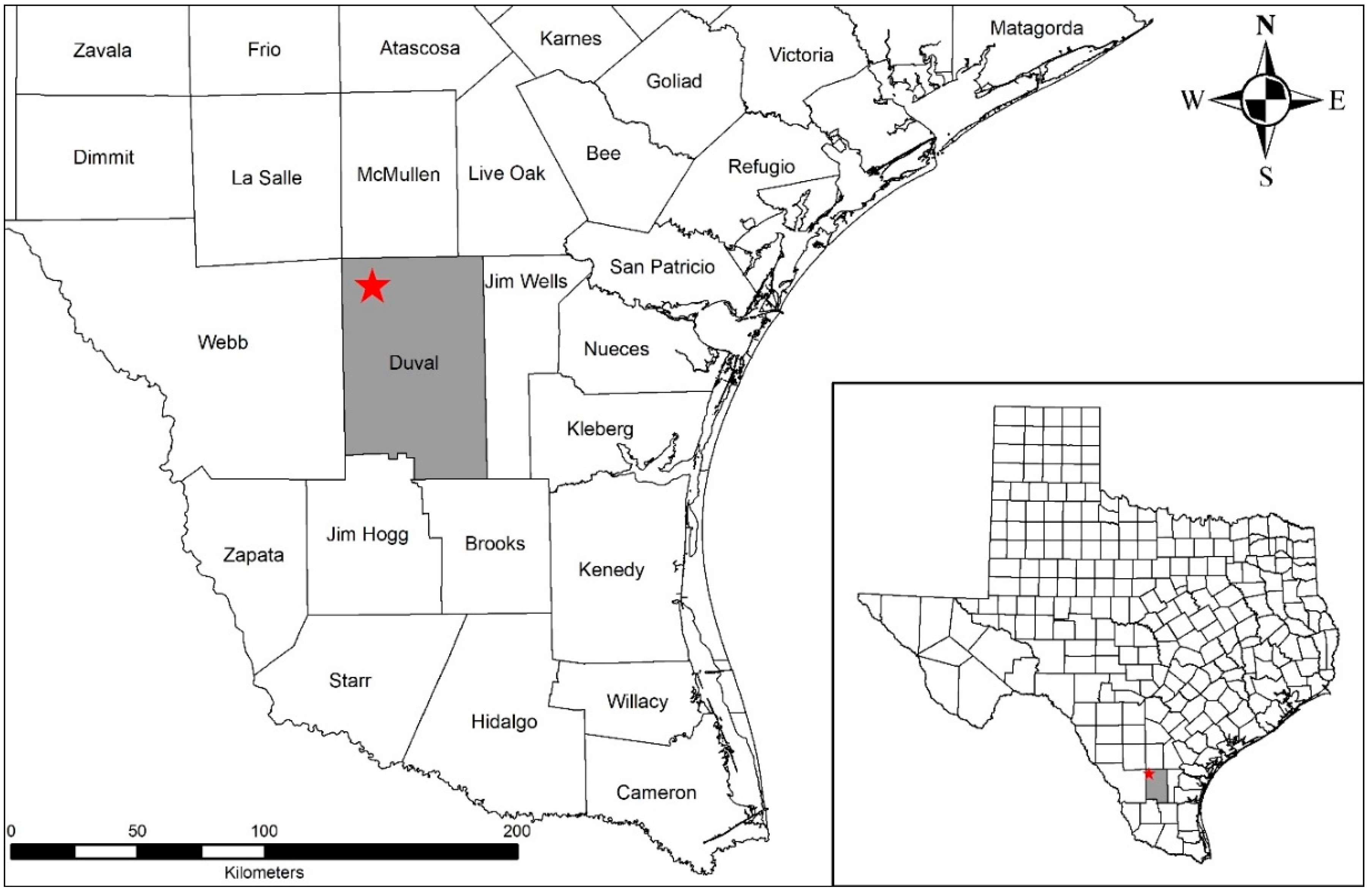
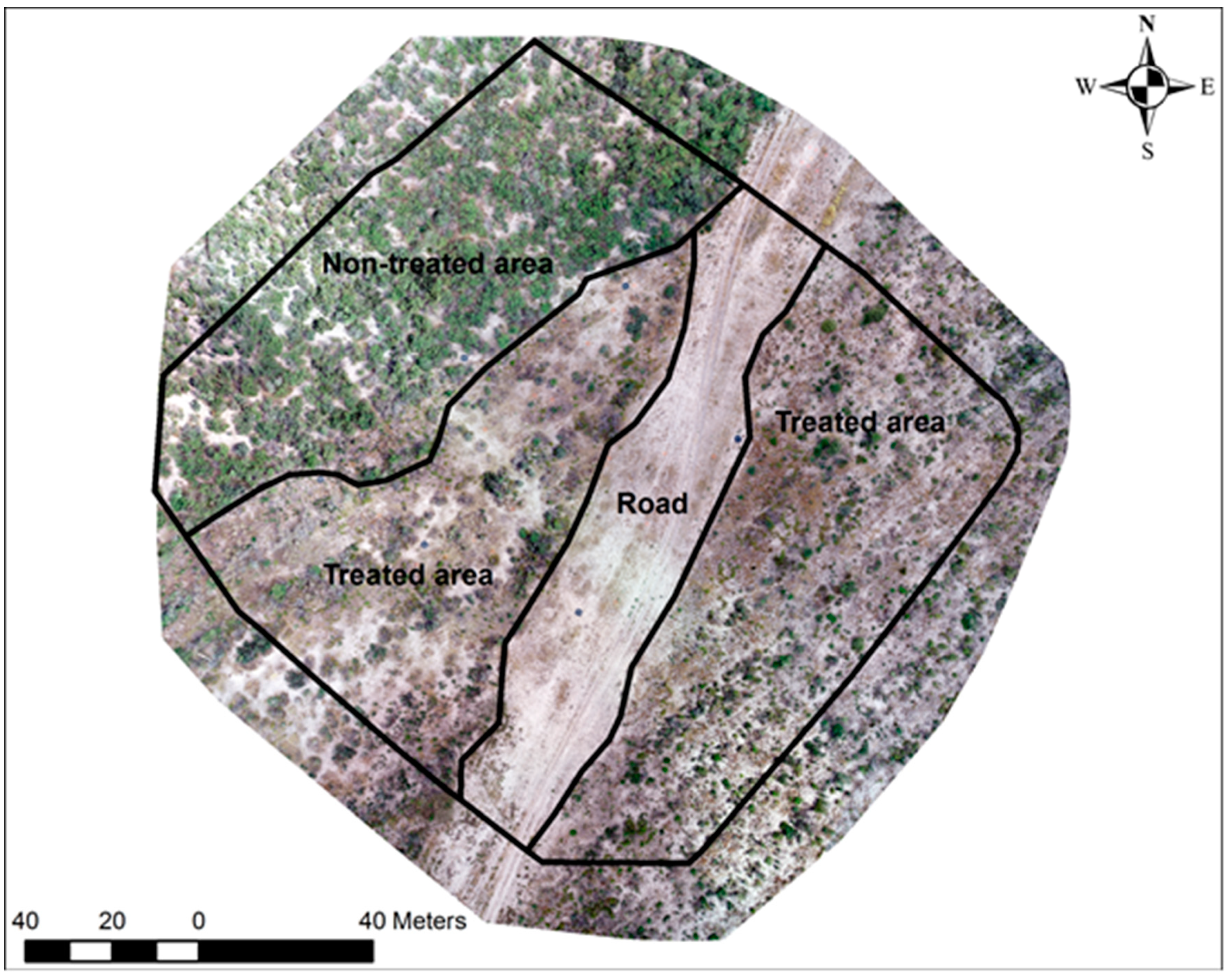
2.1. Study Area

The study site was located in Duval County (Figure 1), on the Duval County Ranch approximately 5 km south of Freer, Texas (27.79194°, −98.73612°). The ranch is in the South Texas Plains ecoregion and has a hot semi-arid climate [37,38]. Mean annual precipitation was 659 mm and mean high and low temperatures were 28.5 °C and 15.3 °C, respectively, during the period 1981–2010 in Freer, Texas [39]. The vegetation had a low percent moisture due to lack of rainfall for approximately 8 weeks prior to sampling and temperatures above 35 °C [39]. Most of the site (75%) consists of Salco fine sandy loam soils, with 1–3% slopes. The remaining 25% is comprised of sandy clay loam soils [40]. The study site is located within the Gray Sandy Loam (R083CY019TX) ecological site (ESD) [41]. Dominant grasses include pink pappusgrass (Pappophorum bicolor Fourn.), plains bristlegrass (Setaria leucopila (Scribn. and Merr.) K. Schum), tanglehead (Heteropogon contortus (L.) P. Beauv. ex Roem. & Schult.), silver bluestem (Bothriochloa laguroides (DC.) Herter), hooded windmillgrass (Chloris cucullata Bisch.), and multiflowered false rhodesgrass (Trichloris pluriflora Fourn.). Woody plants include mottes of honey mesquite (Prosopis glandulosa Torr.) accompanied mainly with scattered brasil (Condalia hookeri M.C. Johnst.), blackbrush acacia (Acacia rigidula Benth.), cenizo (Leucophyllum frutescens (Berl.) I.M. Johnst.), elbowbush (Forestiera angustifolia Torr.), and granjeno (Celtis pallida (Torr.) [41,42,43].

2.2. Image Acquisition

The study site was 2.3 ha and contained an area of herbicide-treated brush (treated in June 2012 with the herbicide Sendero; 54% of total area), a control area (non-treated; 29% of total area), and a road area (2-track dirt road; 17% of total area) (Figure 2). No points were selected in the non-treated area due to scarceness of herbaceous vegetation: only the treated area and the road area were used to estimate forage mass. The flight took place on a sunny, clear day (31 August 2018) with wind speeds <16 km/h. We tested three altitudes: 30 m, 40 m, and 50 m aboveground level (AGL) using a DJI Phantom 4 Pro™ UAV [44]. The UAV unit has an integrated GPS/GLONASS system (Global Positioning System/GLObal NAvigation Satellite System), allowing for faster, more precise satellite acquisition during flights. Natural color aerial images (red, green, blue bands) were taken from a 2.5 cm, 20-megapixel camera mounted to a gimbal that stabilized the camera with the movement of the UAV (pitch, roll, and yaw). Maximum winds were recorded for each flight with a Skywatch Meteos windmeter anemometer (30 m AGL flight = 5 km/h; 40 m AGL flight = 15 km/h; 50 m AGL flight = 7 km/h). Our lowest flight altitude was 30 m AGL; this altitude was used in a similar study for agricultural crops in the same region [45] and we increased the altitude by 10 m increments up to 50 m AGL. This allowed us to assess the effect of pixel resolution on forage estimation. At the time of our flights (August 2018), Cunliffe et al. [25] reported flight altitudes of 20 m AGL. More recently, Gillan et al. [6,26] reported flights for biomass estimation of 20 m and 40 m AGL. For our study we set our flight settings to a double grid style flight pattern, at a speed of 3–5 km/h, 70° camera angle, with 80% image overlap using the Pix4D capture application for Android. The use of convergent image networks to develop photogrammetric models using structure for motion can help improve the reconstruction accuracy of these models [25,45,46]. The UAV flight was controlled through auto-pilot mode in this program. The 30 m flight was separated into two flights because of the increased flight path and 20-min battery limit for the UAV. We used a Trimble GeoXH 6000 GPS unit (10 cm accuracy) and 6 ground control points placed within the perimeter of the plot. Ground control points were used to increase the precision of the georeferenced positioning of the images, increasing the resolution of our models [46].

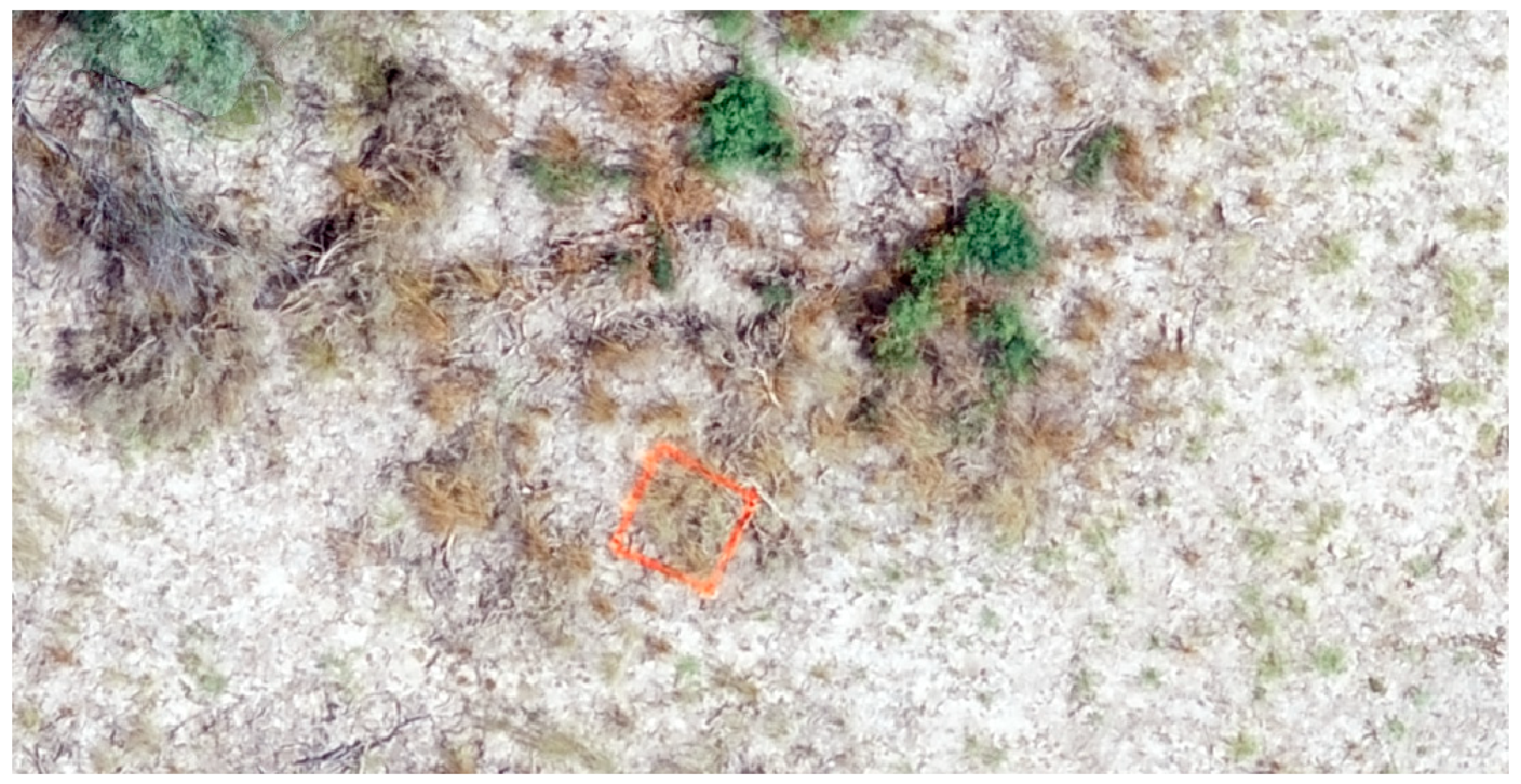
2.3. Field Data Collection

To estimate forage mass using UAV imagery, we conducted a double sampling method similar to the one described by Montalvo et al. [35]. For our pilot study, we placed 20 quadrats (0.5 × 0.5 m) in areas ranging from the lowest production (bare ground) to areas of highest production to represent the range of forage mass. We used the definition of Allen et al. [1] and quantified forage mass as the as the amount for forage above the ground level. The areas used to quantify forage mass were selected following the same criteria used for the double sampling methodology [35,36]. Therefore, no woody cover was included in the forage mass estimations. For each quadrat, percent cover for each species was recorded by visual estimation. The area immediately surrounding the perimeter of the frame was painted bright orange to be visible in the UAV aerial imagery (Figure 3). After the UAV flights were completed, all of the vegetation within each of the 20 quadrats was clipped and weighed to determine forage mass. For each quadrat, a small sample (100 g) was collected and dried to a constant weight to determine percent moisture. Percent moisture for the clipped vegetation was applied to the mass recorded for the quadrat to estimate the dry forage mass in kg/ha [47].

2.4. Image Processing and Volume Estimation

Each flight dataset was processed in Pix4DMapper [48] photogrammetry software to create georeferenced 2D maps and 3D models of the site. We captured 412 images at 30-m AGL, 213 images at 40-m AGL, and 172 images at 50-m AGL. More images were obtained at lower elevations because the camera’s field of view decreases as the UAV gets closer to the ground. For each image dataset, the initial processing consisted of importing and configuring the images by setting up the geolocation (coordinate system, geolocation, and orientation). Camera model parameters were imported from the imagery metadata and ground control points were manually imported into Pix4D [49]. We recorded ground control points using a Trimble GeoXH 6000 with 10 cm horizontal and vertical accuracy with a real-time correction VRS network. We increased our geo-referencing accuracy of the model using the ground control point editor in Pix4D. We selected the 3D model processing option in Pix4D, this option uses imagery with high overlap and oblique aerial imagery. Pix4D uses structure from motion (SfM) photogrammetry for 3D natural environment reconstructions [50]. This generates an orthomosaic and a digital surface model (DSM) that we used to identify height values within the quadrats [51]. We reported the mean (X, Y, Z) root mean square error (RMSE) for each flight.

We delineated the area corresponding to the field quadrats in ArcMap 10.5.1 [52] from the orthomosaic (Figure 2). We then clipped the DSM using the delineated areas within each field quadrat (Figure 3). Vegetation height was calculated by selecting the bare soil lowest point in the DSM within the field quadrat as the base elevation for height estimation. We estimated forage volume (cm³) by multiplying the height value from each pixel and the pixel dimensions, and then adding all volume values within the quadrat [25].

2.5. Statistical Analyses

Forage mass was regressed on vegetation volume using simple linear regression models for each flight altitude. Linear and curvilinear relationships between forage mass and vegetation volume were modeled with logarithmic transformations of forage mass, vegetation volume, or both variables [53,54]. Models were selected by comparing coefficients of determination and model specification was assessed with White’s method [55]. We report models with the highest r² values; all models are included in the supplementary material file (S1). For model validation, we calculated the prediction coefficient of determination (prediction r²) and the PRESS statistic [56].

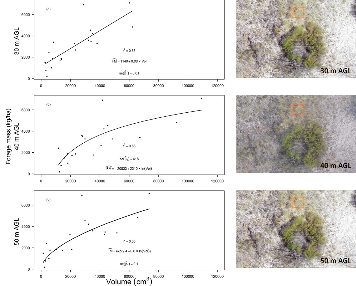
2.6. Forage Mass Estimation

After we calculated the regression equation [35], this was used to estimate forage mass by generating 6 transects and randomly selecting 100 frames (area = 0.25 m²) within the study area. We selected 66 frames in the treated areas and 34 frames in the road area to estimate the average volume. This follows the double sampling methodology to collect data in the field [35]. We averaged the forage mass values for each area and compared our results to an interdependent visual observation conducted by expert opinion (J. A. Ortega S. pers. comm.). Although the expert opinion did not provide individual transect information, the overall values reported provide a comparison of values obtained in the field and with UAVs.

3. Results

Species recorded within our quadrats were: pink pappusgrass, multiflowered false rhodesgrass, plains bristlegrass, common broomweed (Amphiachyris dracunculoides DC. Nutt), tumble lovegrass (Eragrostis sessilispica Buckl.), and an unknown sand mat (Chamaesyce sp.) (

Table 1. Individual species canopy cover for the 20 quadrat frames (area = 0.25 m²) to represent the range of forage mass.

Species Canopy Cover (%)
Quadrat	Pink Pappusgrass	Common Broomweed	Tumble Lovegrass	Multiflowered False Rhodesgrass	Plains Bristlegrass	Sand Mat
1	65	0	0	0	0	0
2	20	0	0	0	0	0
3	70	0	0	0	0	0
4	0	40	0	0	0	0
5	0	0	0	70	0	0
6	30	0	0	0	0	0
7	40	0	0	0	0	0
8	15	25	0	0	0	0
9	80	0	0	0	0	0
10	100	0	0	0	0	0
11	0	0	45	0	0	0
12	15	65	0	0	0	0
13	25	0	0	0	0	0
14	95	0	0	0	0	0
15	75	0	0	0	0	0
16	0	0	0	0	30	0
17	65	0	0	0	0	0
18	0	0	0	100	0	15
19	40	0	0	0	0	0
20	0	0	15	0	0	0

). All grasses listed above are considered forage species for livestock (i.e., cattle). These are all common and representative species for this ecological site. The pixel resolution was 0.779 cm² (30 m AGL), 1.364 cm² (40 m AGL), and 2.102 cm² (50 m AGL). The mean RMSE for were 7.1 cm at 30 m AGL, 6.9 cm at 40 m AGL, and 8.5 cm at 50 m AGL. Field calculated forage mass samples ranged from 184–7082 kg/ha. Volumes obtained from point clouds had a range of 2755–62,265 cm³, 11,763–109,166 cm³, and 3612–73,542 cm³ for the 30 m, 40 m, and 50 m AGL flights, respectively. Regression analyses (Figure 4) and UAV volumes and forage mass have a significant (p < 0.001) relationship at each flight altitude. The greatest r² was obtained with the 30 m AGL flight (r² = 0.65; Figure 4a) and the smallest r² at the 40 m AGL flight (r² = 0.41; S1). Prediction r² values were 0.55, 0.54, and 0.46 for flight heights of 30-, 40-, and 50-m (compared to r² = 0.65, 0.63, and 0.63, respectively), and PRESS statistics were 28%, 24%, and 45% higher than corresponding error sum of squares values for these flight heights.

Average volumes for the road area were 3423 cm³ (30 m AGL), 3446 cm³ (40 m AGL), and 3520 cm³ (50 m AGL); for the treated areas the average volumes were 6599 cm³ (30 m AGL), 7688 cm³ (40 m AGL) and 5293 cm³ (50 m AGL) (

Table 2. Average volumes (cm³) and forage mass estimates (kg/ha) for the road and treated areas in our study area. We did no estimate values for the 40 m AGL as our observed data was outside the minimum observed value for the regression.

Flight Altitude	Road Area		Treated Area
	Average Volume (cm3)	Forage Mass (kg/ha)	Average Volume (cm3)	Forage Mass (kg/ha)
30 m AGL	3423	1413	6599	1667
40 m AGL	3446		7688
50 m AGL	3520	1479	5293	1890

). Forage mass estimates obtained from these average volumes using the regression equations at 30 m AGL were 1413 kg/ha (road area; Figure 4a) and 1667 kg/ha (treated area; Figure 4a). Forage mass estimations at 50 m AGL were 1479 kg/ha (road area; Figure 4c), and 1890 kg/ha (treated area; Table 2). We did not estimate forage mass values (Section 2.5) at 40 m AGL because the minimum observed value for the regression was 11,763 cm³ and the maximum values for the road and treated area were 3445 cm³ and 7687 cm³ which were outside the range of the observed data. Expert opinion values reported 1300 kg/ha for the road area and 1800 kg/ha for the treated area.

4. Discussion

Digital surface models derived from UAV imagery can be used to estimate forage mass on rangelands. For our pilot study, we sampled a digital surface model in a similar way to the double sampling methodology applied in the field. Estimated forage mass obtained from high spatial resolution data is positively related to forage volume. To our knowledge, this is one of the first studies conducted in a semi-arid rangeland to compare flight altitudes for forage mass estimation using high resolution imagery derived from an UAV and sampling imagery in a similar way to field-based methodologies (i.e., double sampling method). Cunliffe et al. [25] used a similar approach to quantify dryland vegetation structure and reported r² values ranging between 0.64 and 0.95. More recently, Gillan et al. [6] reported r²; values ranging between 0.78 and 0.81. Several studies have been conducted to estimate biomass in agricultural crops. For example, Walter et al. [57] found r² = 0.79 in estimated crop biomass of barley (Hordeum vulgare L.), Bendig et al. [32] found r² = 0.92 in estimated wheat (Triticum aestivum) biomass, and Li et al. [29] reported r² = 0.74 for maize (Zea mays) biomass estimation using UAV imagery. Because of the homogeneity of crops, these studies achieved more accurate results using canopy height models compared to volumes derived from point clouds. A study conducted in a semi-desert steppe grassland also found the mean canopy height model presented a strong relationship (R² = 0.76) to above ground biomass [5]. Uniformity of vegetation structure within this grassland was similar to the characteristics of the crop studies listed. Unlike the study areas of Zhang et al. [5], our study was a heterogeneous landscape in terms of forage mass. We identified six species with different plant architectures. While most of our measured transects had 1–2 species (Table 1), the different plant architectures could affect image capture due to poor modelling of plant extremities which created a higher level of heterogeneity than monocultures and could explain our relatively lower r² values [26]. Therefore, we chose to work with forage mass volume derived from entire quadrats rather than individual plant heights within quadrats.

Forage mass estimates between the 30 m AGL and the 50 m AGL were within 250 kg/ha (0.025 kg/m²) of each other. Our results and the values from expert opinion are within 200 kg/ha on both areas. This difference represents a forage mass of 0.02 kg/m². One animal unit equivalent (454 kg cow) consumes 11.8 kg/day [58], therefore these differences are insignificant compared to daily animal consumption. This difference in values obtained from the drone flights and expert opinion are considered acceptable for ranch managers and landowners when estimating correct stocking rates [59]. Our statistical model validation, however, indicated that further research is needed to improve model prediction. Therefore, larger areas can be covered when conducting a 50 m AGL flight using a UAV. This provides the possibility of larger sample areas and potentially larger sample sizes for forage mass estimation. Previous studies have used 20 m AGL [26] and 40 m [6] to cover smaller areas compared to our study area. Further studies should consider higher altitudes and the potential allometric effects on volume estimation [60]. The response of estimated forage mass to changes in forage volume depended on flight altitude. At the lowest (30 m) flight altitude, estimated forage mass increased linearly as forage volume increased. For example, as forage volume increased 10,000 cm³, estimated forage mass increased 800 kg/ha, and this change was constant across forage volume. At a 40-m flight altitude, estimated forage mass increased linearly for a given proportional change in forage volume, e.g., estimated forage mass increased 515 kg/ha for each 25% increase (e.g., 40,000 to 50,000 cm³) in forage volume. At the 50-m flight altitude, however, estimated forage mass changed proportionally for a given proportional change in forage volume; e.g., forage volume increased 14% for each 25% (e.g., 40,000 to 50,000 cm³) increase in forage volume. At higher altitudes, pixel size increases and resolution decreases, therefore, smaller volumes and the top canopy of grasses are less detectable. Gillan et al [6] reported a difference between field measurements of Arizona cottontop (Digitaria californica) and point cloud data estimates at 40 m AGL. We did not include the 40 m AGL for biomass estimation because wind conditions (winds > 7.5 km/h) during that flight affected the co-localization of herbaceous vegetation points. We attribute the observed differences to greater wind speeds during the 40 m AGL flight, which in turn caused the vegetation shape to vary between images. Similar findings were expressed by Walter et al. [56] and led to poor co-localization of points that caused holes in the final point cloud. Because of the sensitivity of grassland vegetation to wind and the resulting distortions in remotely acquired data, weather precautions and multiple flights with high densities of image capture are recommended to ensure data quality. Reviewing weather data to identify number of flying days per year can help plan and maximize the number of flights that can be planned annually and by seasons to estimate forage mass.

To obtain the height measurements of the vegetation to calculate volumes, we used the lowest bare soil elevation point within the quadrat. We chose this approach because we wanted to sample our imagery using a similar approach to the double sampling method [35,36] and not measure every pixel in the landscape. This would allow us to transfer this methodology to the field and add to current efforts in field sampling of forage mass estimation for livestock in heterogeneous rangelands. By using the measurement of quadrats, we can aggregate the information and obtain estimates that are closer to current field estimates. Other studies have used a pixel-by-pixel approach by comparing digital surface models and digital terrain models to estimate plant height [6,25]. These methodologies measure the volume of every pixel and require very high accuracies and very small RMSE values to be able to obtain good estimates [6]. These approaches would require additional effort to classify and remove woody vegetation cover existing imagery to estimate forage mass. Additionally, this would require an accuracy assessment for woody vegetation cover classification, which is impractical and complicated for most landowners, ranch managers, and practitioners who are seeking to adopt UAV technology for forage mass estimation.

Testing different altitudes is important to understand the relationship between pixel resolution and field data for forage mass estimation. Currently transect or quadrat aggregated estimations provide better results than pixel-to-pixel estimations [6]. Improved camera resolution and the use of RTK mounted UAVs may provide more accurate DSM and digital terrain model generation. Flight times are currently a limitation as battery times in quadcopters are less than 30 min. As technology improves, new UAVs will have longer battery times (e.g., Matrice 300 RTK UAV). In order to make this approach operational at larger scales, multiple flights can be conducted in a pasture, selecting the areas prior to the flights. Increased flight altitudes could also provide large area coverage, higher sampling numbers and potentially more precise forage mass estimations. New software development for data capture is now allowing for repeatability of operations, making it easier to assess and monitor changes in vegetation, forage mass availability, and pasture utilization [6,26]. Combined with streamlined workflows these approaches could be very beneficial to support monitoring, and decision making in rangelands. Although large scale pasture sampling analysis is still a limitation, UAVs present an option to current field methods and the development of practical approaches will be key for the adoption of UAVs to support rangeland ecology and management in the near future.

5. Conclusions

Our pilot study showed that UAV technology has the potential to estimate forage mass in rangelands using similar approaches to those currently used in the field. By virtue of the increased number of samples that UAVs can allow, more precise estimates of forage mass can be acquired; equally important, however, is accuracy of estimation. Although expert opinion provided comparable practical results, in view of the fact that our estimated coefficients of determination were < 0.66 and our prediction coefficients of determination were < 0.55, estimating forage mass via our methodology will require additional refinement if higher accuracy is needed for a particular research or management goal. Our data indicate that flying at 50 m AGL will increase the area covered without compromising the accuracy of the forage mass estimation. Testing higher altitudes (e.g., 100 m AGL) could bring this approach closer to deployment at the pasture scale. This would help collect several hundred quadrats along larger areas to estimate forage mass at the pasture scale. The use of UAV technology in the future will provide greater opportunities for management applications in rangelands. Future studies need to consider different ecosystems, seasons, data collection parameters and automation techniques to develop robust methodologies that can be translated into management tools for rangeland practitioners. UAV approaches will not replace current field techniques, but will improve the capabilities of field data collection, particularly in rough terrain. It will also allow for the efficient large-scale analysis of rangelands that are highly beneficial to landowners, ranchers, and rangeland practitioners to aid in stocking rate decisions, and for the monitoring and assessment of rangelands.

References

1. Allen, V.G.; Batello, C.; Berretta, E.J.; Hodgson, J.; Kothmann, M.; Li, X.; McIvor, J.; Milne, J.; Morris, C.; Peeters, A.; et al. An international terminology for grazing lands and grazing animals. Grass Forage Sci. 2011, 66, 2–28. [Google Scholar] [CrossRef]
2. Brummer, J.E.; Nichols, J.T.; Engel, R.K.; Eskridge, K.M. Efficiency of different quadrat sizes and shapes for sampling standing crop. J. Range Manag. 1994, 47, 84–89. [Google Scholar] [CrossRef]
3. Byrne, K.; Lauenroth, W.; Adler, P.; Byrne, C. Estimating Aboveground Net Primary Production in Grasslands: A Comparison of Nondestructive Methods. Rangel. Ecol. Manag. 2011, 64, 498–505. [Google Scholar] [CrossRef]
4. Catchpole, W.R.; Catchpole, E.A. Stratified Double Sampling of Patchy Vegetation to Estimate Biomass. Biometrics 1993, 49, 295–303. [Google Scholar] [CrossRef]
5. Zhang, H.; Sum, Y.; Chang, L.; Qin, Y.; Du, J.; Yi, S.; Wang, Y. Estimation of grassland Canopy Height and Aboveground Biomass at the Quadrat Scale Using Unmanned Aerial Vehicle. Remote Sens. 2018, 10, 851. [Google Scholar] [CrossRef] [Green Version]
6. Gillan, J.K.; McClaran, M.P.; Swetnam, T.L.; Heilman, P. Estimating forage utilization with drone-based photogrammetric point clouds. Rangel. Ecol. Manag. 2019, 72, 575–585. [Google Scholar] [CrossRef]
7. Glasscock, S.N.; Grant, W.E.; Draw, D.L. Simulation of vegetation dynamics and management strategies on south Texas, semi-arid rangeland. J. Environ. Manag. 2005, 75, 379–397. [Google Scholar] [CrossRef]
8. Fuhlendorf, S.D.; Briske, D.D.; Smeins, F.E. Herbaceous vegetation change in variable rangeland environments: The relative contribution of grazing and climatic variability. Appl. Veg. Sci. 2001, 4, 177–188. [Google Scholar] [CrossRef]
9. Chen, W.; Blain, D.; Li, J.; Koehler, K.; Fraser, R.; Zhang, Y.; Leblanc, S.; Olthof, I.; Wang, J.; McGovern, M. Biomass measurements and relationships with Landsat-7/ETM+ and JERS-1/SAR data over Canada’s western sub-arctic and low arctic. Int. J. Remote Sens. 2009, 30, 2355–2376. [Google Scholar] [CrossRef]
10. Gibb, M.J.; Ridout, M.S. The fitting of frequency distributions to height measurements on grazed swards. Grass Forage Sci. 1986, 41, 247–249. [Google Scholar] [CrossRef]
11. Holechek, J.L.; Pieper, R.D.; Herbel, C.H. Range Management: Principles and Practices, 6th ed.; Pearson: New York, NY, USA, 2011; pp. 169–201. [Google Scholar]
12. Illius, A.W.; Wood-Gush, D.G.M.; Eddison, J.C. A study of the foraging behavior of cattle grazing patchy swards. Biol. Behav. 1987, 12, 33–44. [Google Scholar]
13. Tsutsumi, M.; Itano, S.; Shiyomi, M. Number of Samples Required for Estimating Herbaceous Biomass. Rangel. Ecol. Manag. 2007, 60, 447–452. [Google Scholar] [CrossRef]
14. Bonham, C.D. Measurements for Terrestrial Vegetation, 2nd ed.; John Wiley and Sons: West Sussex, UK, 2013; pp. 175–199. [Google Scholar]
15. Laliberte, A.S.; Herrick, J.E.; Rango, A.; Winters, C. Acquisition, orthorectification, and object-based classification of unmanned aerial vehicle (UAV) imagery for rangeland monitoring. Photogramm. Eng. Remote Sens. 2010, 76, 661–672. [Google Scholar] [CrossRef]
16. Castillo-Santiago, M.; Ricker, M.; Bernardus, J. Estimation of tropical forest structure from SPOT5 satellite images. Int. J. Remote Sens. 2010, 31, 2767–2782. [Google Scholar] [CrossRef]
17. Everitt, J.H.; Anderson, G.L.; Escobar, D.E.; Davis, M.R.; Spencer, N.R.; Andrascik, R.J. Use of remote sensing for detecting and mapping leafy spurge (Euphorbia esula). Weed Technol. 1995, 9, 599–609. [Google Scholar] [CrossRef] [Green Version]
18. Mata, J.; Perotto-Baldivieso, H.L.; Hernández, F.; Grahmann, E.D.; Rideout-Hanzak, S.; Edwards, J.T.; Page, M.T.; Shedd, T.M. Quantifying the spatial and temporal distribution of tanglehead (Heteropogon contortus) on South Texas rangelands. Ecol. Process. 2018, 7, 2. [Google Scholar] [CrossRef] [Green Version]
19. Kumar, L.; Sinha, P.; Taylor, S.; Alqurashi, A. Review of the use of remote sensing for biomass estimation to support renewable energy generation. J. Appl. Remote Sens. 2015, 9, 097696. [Google Scholar] [CrossRef]
20. Dube, T.; Mutanga, O. Evaluating the utility of the medium-spatial resolution Landsat 8 multispectral sensor in quantifying aboveground biomass in uMgeni catchment, South Africa. ISPRS J. Photogramm. Remote Sens. 2015, 101, 36–46. [Google Scholar] [CrossRef]
21. Grant, K.M.; Johnson, D.L.; Hildebrand, D.V.; Peddle, D.R. Quantifying biomass production on rangeland in southern Alberta using SPOT imagery. Can. J. Remote Sens. 2013, 38, 695–708. [Google Scholar] [CrossRef]
22. Kross, A.; McNairn, H.; Lapen, D.; Sunohara, M.; Champagne, C. Assessment of RapidEye vegetation indices for estimation of leaf area index and biomass in corn and soybean crops. Int. J. Appl. Earth Obs. Geoinf. 2015, 34, 235–248. [Google Scholar] [CrossRef] [Green Version]
23. Shoko, C.; Mutanga, O.; Dube, T. Progress in the remote sensing of C3 and C4 grass species aboveground biomass over time and space. ISPRS J. Photogramm. Remote Sens. 2016, 120, 13–24. [Google Scholar] [CrossRef]
24. Manfreda, S.; McCabe, M.F.; Miller, P.E.; Lucas, R.; Madrigal, V.P.; Mallinis, G.; Ben Dor, E.; Helman, D.; Estes, L.; Ciraolo, G.; et al. On the Use of Unmanned Aerial Systems for Environmental Monitoring. Remote Sens. 2018, 10, 641. [Google Scholar] [CrossRef] [Green Version]
25. Cunliffe, A.M.; Brazier, R.E.; Anderson, K. Ultra-fine grain landscape-scale quantification of dryland vegetation structure with drone-acquired structure-from-motion photogrammetry. Remote Sens. Environ. 2016, 183, 129–143. [Google Scholar] [CrossRef] [Green Version]
26. Gillan, J.K.; Karl, J.W.; van Leeuwen, W.J.D. Integrating drone imagery with existing rangeland monitoring programs. Environ. Monit. Assess. 2020, 192, 269. [Google Scholar] [CrossRef] [PubMed]
27. Bendig, J.; Bolten, A.; Bennertz, S.; Broscheit, J.; Eichfuss, S.; Bareth, G. Estimating biomass of barley using crop surface models (CSMS) derived from UAV-based RGB imaging. Remote Sens. 2014, 6, 10395–10412. [Google Scholar] [CrossRef] [Green Version]
28. Tilly, A.N.; Hoffmeister, D.; Cao, Q.; Huang, S.; Lenz-Wiedemann, V.; Miao, Y.; Bareth, G. Multitemporal crop surface models: Accurate plant height measurement and biomass estimation with terrestrial laser scanning in paddy rice. J. Appl. Remote Sens. 2014, 8, 083671. [Google Scholar] [CrossRef]
29. Li, W.; Niu, Z.; Chen, H.; Li, D.; Wu, M.; Zhao, W. Remote estimation of canopy height and aboveground biomass of maize using high-resolution stereo images from a low-cost unmanned aerial vehicle system. Ecol. Indic. 2016, 67, 637–648. [Google Scholar] [CrossRef]
30. Souza, C.H.W.D.; Lamparelli, R.A.C.; Rocha, J.V. Height estimation of sugarcane using an unmanned aerial system UAS based on structure from motion SFM point clouds. Int. J. Remote Sens. 2017, 38, 2218–2230. [Google Scholar] [CrossRef]
31. Wallace, L.; Lucieer, A.; Malenovský, Z.; Turner, D.; Vopěnka, P. Assessment of forest structure using two UAV techniques: A comparison of airborne laser scanning and structure from motion (SfM) point clouds. Forests 2016, 7, 62. [Google Scholar] [CrossRef] [Green Version]
32. Bendig, J.; Yu, K.; Aasen, H.; Bolten, A.; Bennertz, S.; Broscheit, J.; Gnyp, M.L.; Bareth, G. Combining UAV-based plant height from crop surface models, visible, and near infrared vegetation indices for biomass monitoring in barley. Int. J. Appl. Earth Obs. 2015, 39, 79–87. [Google Scholar] [CrossRef]
33. Ku, N.-W.; Popescu, S.; Ansley, R.J.; Perotto-Baldivieso, H.L. Assessment of available rangeland woody plant biomass with a terrestrial lidar system. Photogramm. Eng. Remote Sens. 2012, 78, 349–361. [Google Scholar] [CrossRef]
34. Ten Harkel, J.; Bartholomeus, H.; Kooistra, L. Biomass and Crop Height Estimation of Different Crops Using UAV-Based Lidar. Remote Sens. 2019, 12, 17. [Google Scholar] [CrossRef] [Green Version]
35. Montalvo, A.; Snelgrove, T.; Riojas, G.; Schofield, L.; Campbell, T.A. Cattle ranching in the “Wild Horse Desert”—Stocking rate, rainfall, and forage responses. Rangelands 2020, 42, 31–42. [Google Scholar] [CrossRef]
36. Despain, D.W.; Smith, E.L. The comparative yield method for estimating range production. In Some Methods for Monitoring Rangelands and Other Natural Area Vegetation; Rule, G.B., Ed.; Arizona Cooperative Extension Publication 190043: Tucson, AZ, USA, 1987; pp. 49–90. [Google Scholar]
37. Beck, H.E.; Zimmermann, N.E.; McVicar, T.R.; Vergopolan, N.; Berg, A.; Wood, E.F. Present and future Köppen-Geiger climate classification maps at 1-km resolution. Sci. Data 2018, 5, 180214. [Google Scholar] [CrossRef] [PubMed] [Green Version]
38. Texas Parks and Wildlife. Ecoregions of Texas. 2018. Available online: https://tpwd.texas.gov/education/hunter-education/online-course/wildlife-conservation/texas-ecoregions (accessed on 6 October 2018).
39. U.S. Climate Data. Climate Freer-Texas. 2018. Available online: https://www.usclimatedata.com/climate/freer/texas/united-states/ustx0589 (accessed on 4 October 2018).
40. Web Soil Survey. AOI of Study Site. Available online: https://websoilsurvey.sc.egov.usda.gov/App/WebSoilSurvey.aspx (accessed on 19 June 2020).
41. Ecological Site Description Catalog. Available online: https://edit.jornada.nmsu.edu/page?content=class&catalog=3&spatial=163&class=8418 (accessed on 19 June 2020).
42. Hatch, S.L.; Umphres, K.C.; Ardon, A.J. Field Guide to Common Texas Grasses; Texas A&M University Press: College Station, TX, USA, 2015. [Google Scholar]
43. USDA; NRCS. The PLANTS Database. 2019. Available online: http://plants.usda.gov (accessed on 5 November 2018).
44. DJI. Phantom 4 Pro Information. 2018. Available online: https://www.dji.com/phantom-4-pro/info. (accessed on 20 October 2018.).
45. Garza, B.N.; Ancona, V.; Enciso, J.; Perotto-Baldivieso, H.L.; Kunta, M.; Simpson, C. Quantifying Citrus Tree Health Using True Color UAV Images. Remote Sens. 2020, 12, 170. [Google Scholar] [CrossRef] [Green Version]
46. Sanz-Ablanedo, E.; Chandler, J.H.; Rodríguez-Pérez, J.R.; Ordóñez, C. Accuracy of Unmanned Aerial Vehicle (UAV) and SfM Photogrammetry Survey as a Function of the Number and Location of Ground Control Points Used. Remote Sens. 2018, 10, 1606. [Google Scholar] [CrossRef] [Green Version]
47. Pieper, R.D. Rangeland vegetation productivity and biomass. In Vegetation Science Applications for Rangeland Analysis and Management; Tueller, P.T., Ed.; Springer: Dordrecht, The Netherlands, 1988; pp. 449–467. [Google Scholar]
48. Pix4D. Pix4Dmapper. 2016. Available online: https://www.pix4d.com/product/pix4dmapper-photogrammetry-software (accessed on 10 February 2019).
49. Cubero-Castan, M.; Schneider-Zapp, K.; Bellomo, M.; Shi, D.; Rehak, M.; Strecha, C. Assessment of the Radiometric Accuracy in a Target Less Work Flow Using Pix4D Software. In Proceedings of the 2018 9th Workshop on Hyperspectral Image and Signal Processing: Evolution in Remote Sensing (WHISPERS), Amsterdam, The Netherlands, 23 September 2018; pp. 1–4. [Google Scholar]
50. Burns, J.H.R.; Delparte, D. Comparison of commercial structure-from-motion photogrammetry software used for underwater three-dimensional modeling of coral reef environments. Int. Arch. Photogramm. Remote Sens. Spatial Inf. Sci. 2017, XLII-2/W3, 127–131. [Google Scholar] [CrossRef] [Green Version]
51. Liu, Y.; Zheng, X.; Ai, G.; Zhang, Y.; Zuo, Y. Generating a High-Precision True Digital Orthophoto Map based on UAV images. ISPRS Int. J. Geo-Inf. 2018, 7, 333. [Google Scholar] [CrossRef] [Green Version]
52. ESRI. ArcGIS Desktop: Release 10; Environmental Systems Research Institute: Redlands, CA, USA, 2011. [Google Scholar]
53. Gujarati, D.N.; Porter, D.C. Basic Econometrics, 5th ed.; McGraw Hill Inc.: New York, NY, USA, 2009. [Google Scholar]
54. Sokal, R.R.; James, F.J. Biometry: The Principles and Practice of Statistics in Biological Research, 3rd ed.; W.H. Freeman and Company: New York, NY, USA, 1995. [Google Scholar]
55. White, H.A. Heteroskedasticity-Consistent Covariance Matrix Estimator and a Direct Test for Heteroskedasticity. Econometrica 1980, 48, 817–838. [Google Scholar] [CrossRef]
56. Montgomery, D.C.; Peck, E.A.; Vining, G.G. Introduction to Linear Regression Analysis, 5th ed.; John Wiley & Sons, Inc.: Hoboken, NJ, USA, 2012. [Google Scholar]
57. Walter, J.; Edwards, J.; McDonald, G.; Kuchel, H. Photogrammetry for the estimation of wheat biomass and harvest index. Field Crop. Res. 2018, 216, 165–174. [Google Scholar] [CrossRef]
58. Hanselka, C.W.; White, L.D.; Holechek, J.L. Using forage harvest efficiency to determine stocking rate. Tex. Coop. Ext. 2014, E-128, 2. [Google Scholar]
59. Ortega-S., J.A.; Bryant, F.C. Cattle Management to Enhance Wildlife Habitat; Management Bulletin No. 6; Caesar Kleberg Wildlife Research Institute: Kingsville, TX, USA, 2005; 12p. [Google Scholar]
60. Juecker, T.; Caspersen, J.; Chave, J.; Antin, C.; Barbier, N.; Bongers, F.; Dalponte, M.; Ewijk, K.Y.; Forrester, D.I.; Haeni, M.; et al. Allometric equations for integrating remote sensing imagery into forest monitoring programmes. Glob. Chang. Biol. 2017, 23, 177–190. [Google Scholar] [CrossRef] [PubMed]
Figure 1. Study site location on Duval County Ranch, NW Duval County, TX.
Remotesensing 12 02431 g001
Figure 2. Orthomosaic of the study area obtained at 50 m above ground level on Duval County Ranch in Duval County, TX, 31 August 2018. Black lines represent the boundary between treated areas, non-treated areas, and road.
Remotesensing 12 02431 g002
Figure 3. Orange spray-painted quadrat shown from UAV imagery at Duval County Ranch in Duval County, TX, 31 August 2018.
Remotesensing 12 02431 g003
Figure 4. Regression analysis between forage mass and 3D model volumes from imagery obtained at Duval County Ranch in Duval County, TX, 31 August 2018. Coefficient of determination (r2) and standing forage crop production equation containing estimated regression coefficients are shown for linear-linear regression analysis at 30 m AGL (a), linear-log regression at 40 m AGL (b), and log-log at 50 m AGL (c). AGL denotes height above ground level.
Remotesensing 12 02431 g004