Comparing Sentinel-1 Surface Water Mapping Algorithms and Radiometric Terrain Correction Processing in Southeast Asia Utilizing Google Earth Engine

 , , , ,
Abstract
:
1. Introduction
2. Materials and Methods
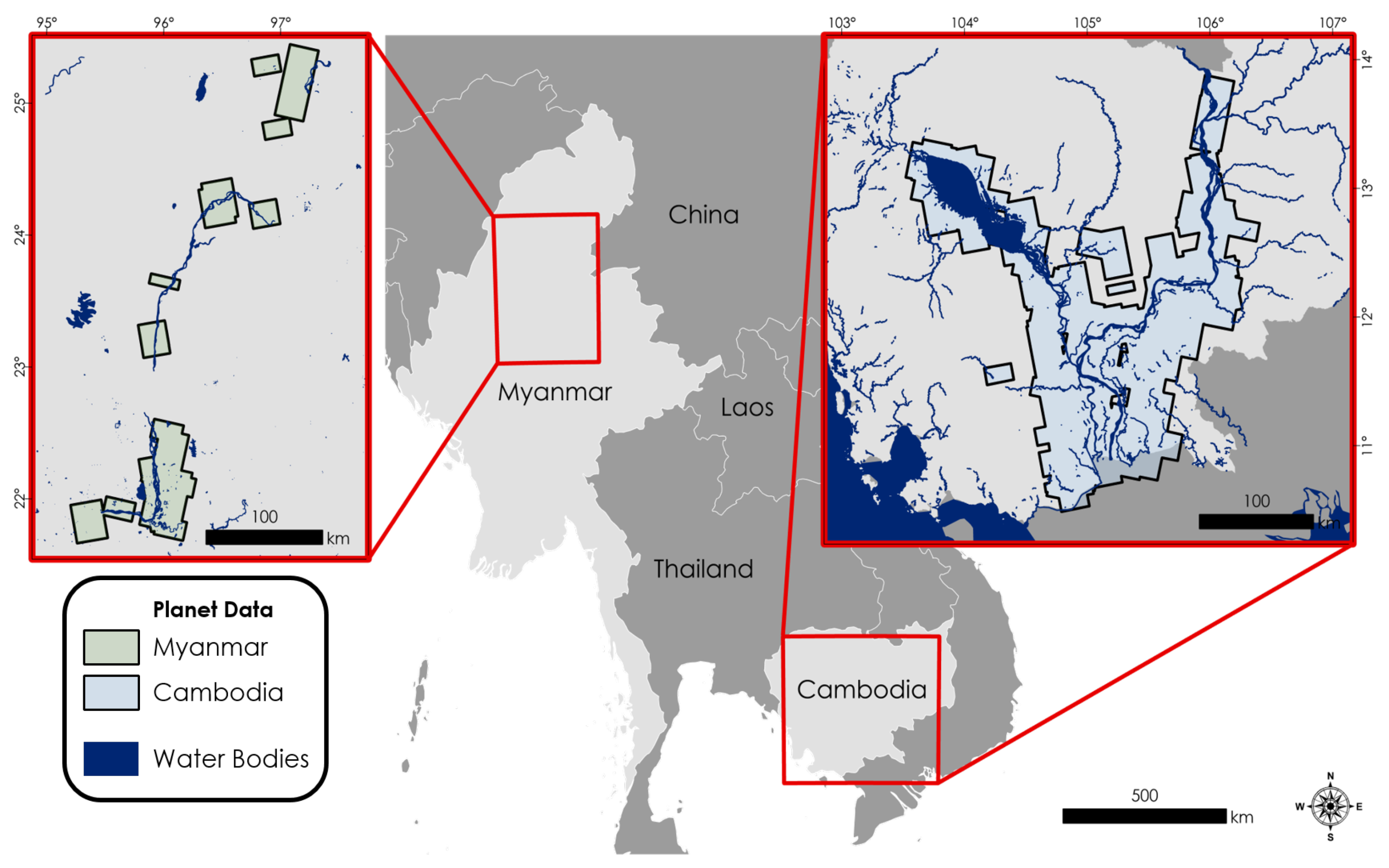
2.1. Study Area and Period
2.2. Data Used
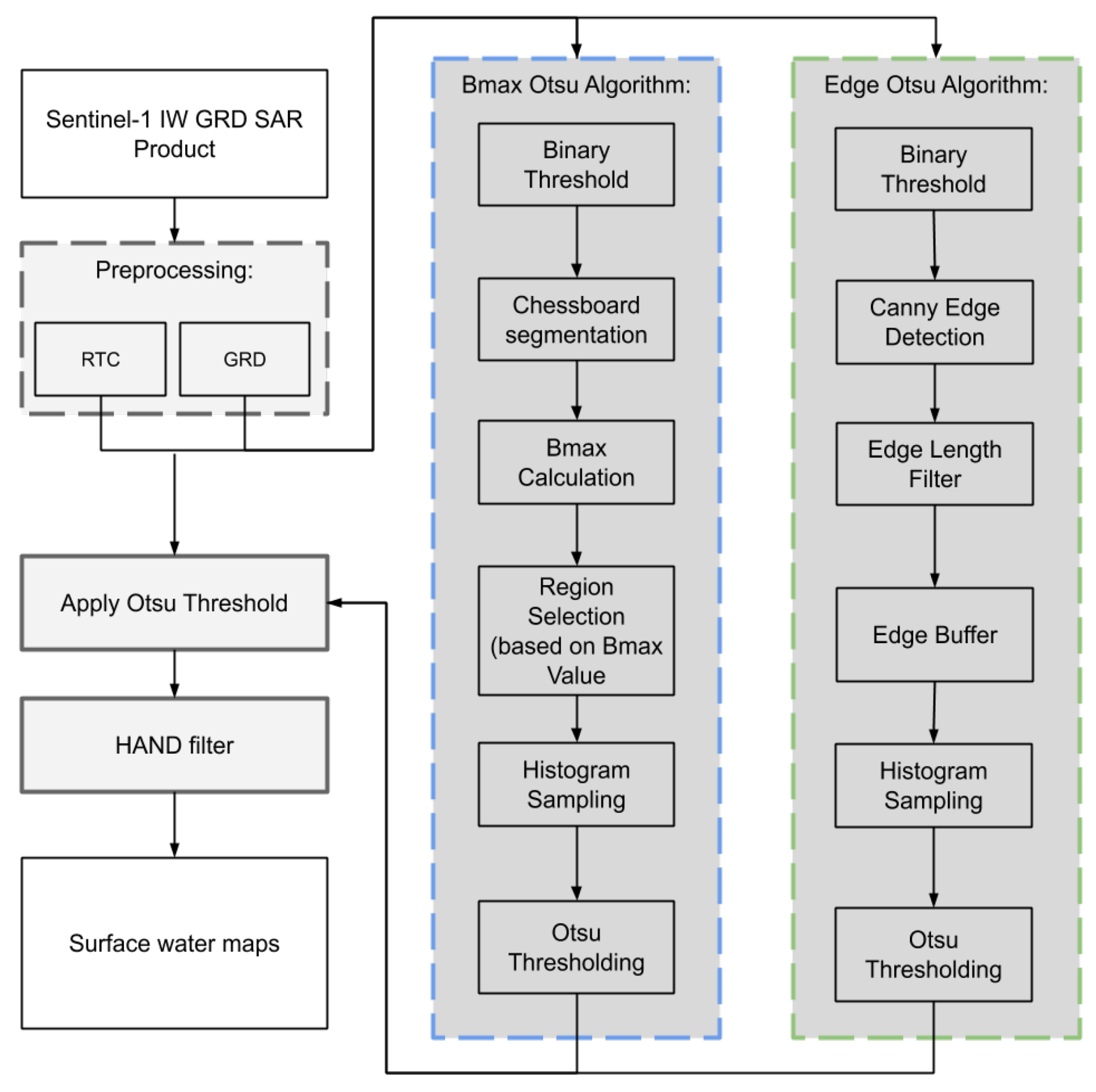
2.2.1. Sentinel-1 Data
2.2.2. MERIT DEM
2.2.3. Planet Scope
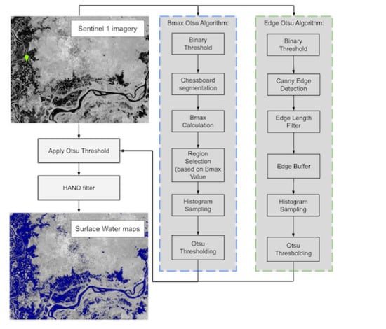
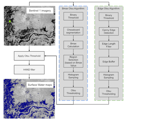
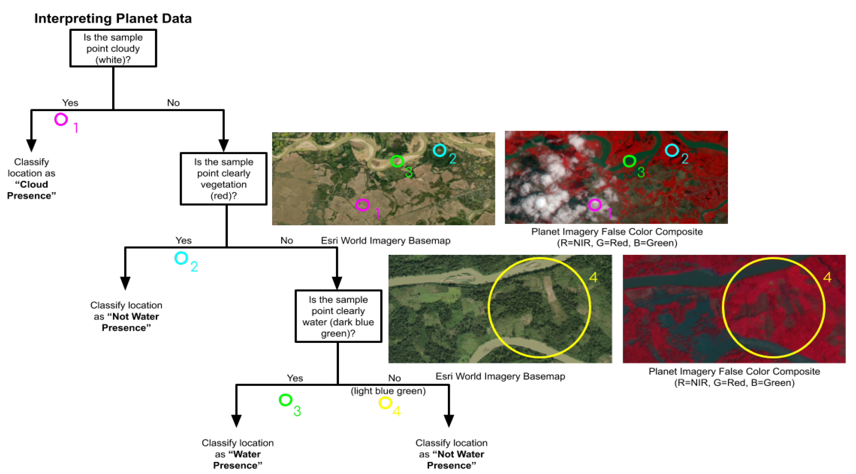
2.3. Surface Water Mapping
2.3.1. Bmax Otsu Algorithm
2.3.2. Edge Otsu Algorithm
2.4. Evaluation Design
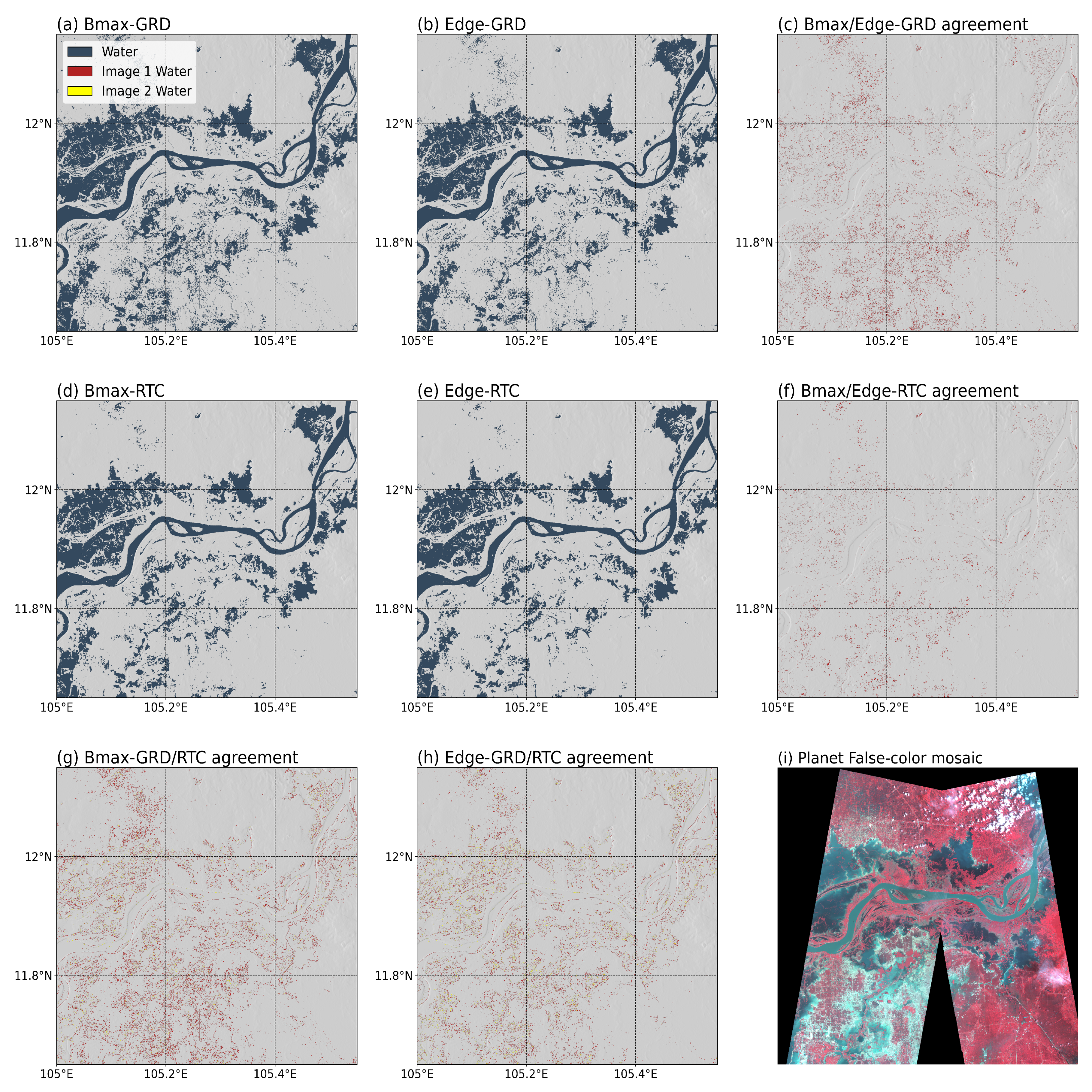
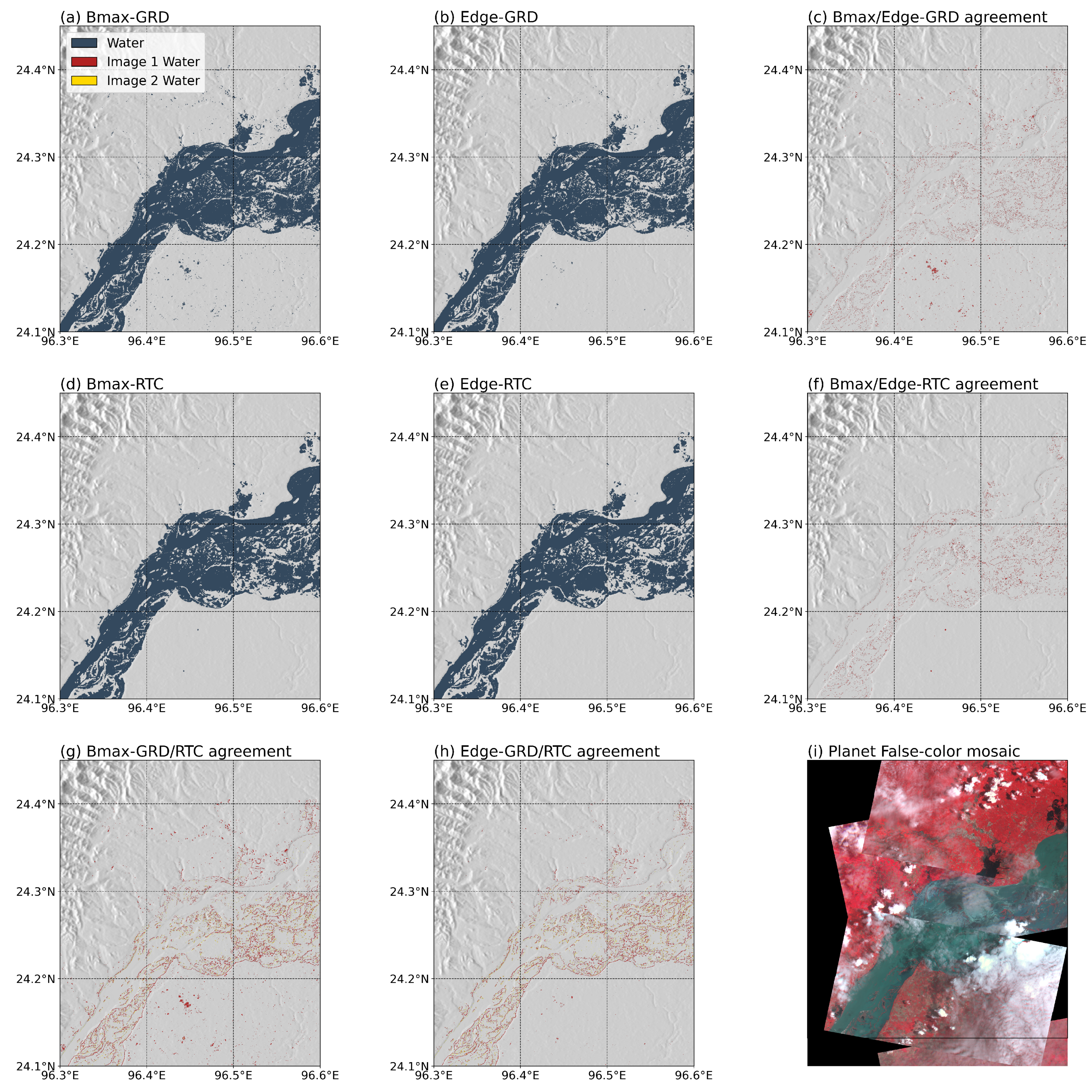
3. Results and Discussion
3.1. Caveats and Limitations
3.2. Future Work
4. Conclusions
Supplementary Materials
Author Contributions
Funding
Acknowledgments
Conflicts of Interest
References
- Ali, M.; Clausi, D. Using the Canny edge detector for feature extraction and enhancement of remote sensing images. In Proceedings of the IEEE 2001 International Geoscience and Remote Sensing Symposium (Cat. No. 01CH37217), Sydney, NSW, Australia, 9–13 July 2001; Volume 5, pp. 2298–2300. [Google Scholar]
- Ahamed, A.; Bolten, J.D. A MODIS-based automated flood monitoring system for southeast asia. Int. J. Appl. Earth Obs. Geoinf. 2017, 61, 104–117. [Google Scholar] [CrossRef] [Green Version]
- Poortinga, A.; Bastiaanssen, W.; Simons, G.; Saah, D.; Senay, G.; Fenn, M.; Bean, B.; Kadyszewski, J. A self-calibrating runoff and streamflow remote sensing model for ungauged basins using open-access earth observation data. Remote Sens. 2017, 9, 86. [Google Scholar] [CrossRef] [Green Version]
- Tolentino, P.L.M.; Poortinga, A.; Kanamaru, H.; Keesstra, S.; Maroulis, J.; David, C.P.C.; Ritsema, C.J. Projected impact of climate change on hydrological regimes in the Philippines. PLoS ONE 2016, 11, e0163941. [Google Scholar] [CrossRef] [PubMed] [Green Version]
- Oddo, P.C.; Bolten, J.D. The Value of Near Real-Time Earth Observations for Improved Flood Disaster Response. Front. Environ. Sci. 2019, 7, 127. [Google Scholar] [CrossRef] [Green Version]
- Liu, C.C.; Shieh, M.C.; Ke, M.S.; Wang, K.H. Flood Prevention and Emergency Response System Powered by Google Earth Engine. Remote Sens. 2018, 10, 1283. [Google Scholar] [CrossRef] [Green Version]
- Du, Z.; Li, W.; Zhou, D.; Tian, L.; Ling, F.; Wang, H.; Gui, Y.; Sun, B. Analysis of Landsat-8 OLI imagery for land surface water mapping. Remote Sens. Lett. 2014, 5, 672–681. [Google Scholar] [CrossRef]
- Ji, L.; Geng, X.; Sun, K.; Zhao, Y.; Gong, P. Target detection method for water mapping using Landsat 8 OLI/TIRS imagery. Water 2015, 7, 794–817. [Google Scholar] [CrossRef] [Green Version]
- Yang, X.; Zhao, S.; Qin, X.; Zhao, N.; Liang, L. Mapping of urban surface water bodies from Sentinel-2 MSI imagery at 10 m resolution via NDWI-based image sharpening. Remote Sens. 2017, 9, 596. [Google Scholar] [CrossRef] [Green Version]
- Yilmaz, K.K.; Adler, R.F.; Tian, Y.; Hong, Y.; Pierce, H.F. Evaluation of a satellite-based global flood monitoring system. Int. J. Remote Sens. 2010, 31, 3763–3782. [Google Scholar] [CrossRef]
- Fayne, J.V.; Bolten, J.D.; Doyle, C.S.; Fuhrmann, S.; Rice, M.T.; Houser, P.R.; Lakshmi, V. Flood mapping in the lower Mekong River Basin using daily MODIS observations. Int. J. Remote Sens. 2017, 38, 1737–1757. [Google Scholar] [CrossRef]
- Huang, C.; Chen, Y.; Zhang, S.; Li, L.; Shi, K.; Liu, R. Surface water mapping from Suomi NPP-VIIRS imagery at 30 m resolution via blending with Landsat data. Remote Sens. 2016, 8, 631. [Google Scholar] [CrossRef] [Green Version]
- Li, S.; Sun, D.; Goldberg, M.D.; Sjoberg, B.; Santek, D.; Hoffman, J.P.; DeWeese, M.; Restrepo, P.; Lindsey, S.; Holloway, E. Automatic near real-time flood detection using Suomi-NPP/VIIRS data. Remote Sens. Environ. 2018, 204, 672–689. [Google Scholar] [CrossRef]
- Xu, H. Modification of normalised difference water index (NDWI) to enhance open water features in remotely sensed imagery. Int. J. Remote Sens. 2006, 27, 3025–3033. [Google Scholar] [CrossRef]
- Feyisa, G.L.; Meilby, H.; Fensholt, R.; Proud, S.R. Automated Water Extraction Index: A new technique for surface water mapping using Landsat imagery. Remote Sens. Environ. 2014, 140, 23–35. [Google Scholar] [CrossRef]
- Zhou, Y.; Dong, J.; Xiao, X.; Xiao, T.; Yang, Z.; Zhao, G.; Zou, Z.; Qin, Y. Open surface water mapping algorithms: A comparison of water-related spectral indices and sensors. Water 2017, 9, 256. [Google Scholar] [CrossRef]
- Jones, J.W. Efficient wetland surface water detection and monitoring via landsat: Comparison with in situ data from the everglades depth estimation network. Remote Sens. 2015, 7, 12503–12538. [Google Scholar] [CrossRef] [Green Version]
- Jones, J.W. Improved automated detection of subpixel-scale inundation—Revised dynamic surface water extent (dswe) partial surface water tests. Remote Sens. 2019, 11, 374. [Google Scholar] [CrossRef] [Green Version]
- Donchyts, G.; Baart, F.; Winsemius, H.; Gorelick, N.; Kwadijk, J.; Van De Giesen, N. Earth’s surface water change over the past 30 years. Nat. Clim. Chang. 2016, 6, 810–813. [Google Scholar] [CrossRef]
- Donchyts, G.; Schellekens, J.; Winsemius, H.; Eisemann, E.; Van de Giesen, N. A 30 m resolution surface water mask including estimation of positional and thematic differences using landsat 8, srtm and openstreetmap: A case study in the Murray-Darling Basin, Australia. Remote Sens. 2016, 8, 386. [Google Scholar] [CrossRef] [Green Version]
- Pekel, J.F.; Cottam, A.; Gorelick, N.; Belward, A.S. High-resolution mapping of global surface water and its long-term changes. Nature 2016, 540, 418–422. [Google Scholar] [CrossRef]
- Isikdogan, F.; Bovik, A.C.; Passalacqua, P. Surface water mapping by deep learning. IEEE J. Sel. Top. Appl. Earth Obs. Remote Sens. 2017, 10, 4909–4918. [Google Scholar] [CrossRef]
- Markert, K.N.; Chishtie, F.; Anderson, E.R.; Saah, D.; Griffin, R.E. On the merging of optical and SAR satellite imagery for surface water mapping applications. Results Phys. 2018, 9, 275–277. [Google Scholar] [CrossRef]
- Sanyal, J.; Lu, X. Application of remote sensing in flood management with special reference to monsoon Asia: A review. Nat. Hazards 2004, 33, 283–301. [Google Scholar] [CrossRef]
- Psomiadis, E. Flash flood area mapping utilising SENTINEL-1 radar data. In Earth Resources and Environmental Remote Sensing/GIS Applications VII. International Society for Optics and Photonics; SPIE Remote Sensing: Edinburgh, UK, 2016; Volume 10005, p. 100051G. [Google Scholar]
- Elkhrachy, I. Assessment and management flash flood in Najran Wady using GIS and remote sensing. J. Indian Soc. Remote Sens. 2018, 46, 297–308. [Google Scholar] [CrossRef]
- Clement, M.; Kilsby, C.; Moore, P. Multi-temporal synthetic aperture radar flood mapping using change detection. J. Flood Risk Manag. 2018, 11, 152–168. [Google Scholar] [CrossRef]
- Amitrano, D.; Di Martino, G.; Iodice, A.; Riccio, D.; Ruello, G. Unsupervised rapid flood mapping using Sentinel-1 GRD SAR images. IEEE Trans. Geosci. Remote Sens. 2018, 56, 3290–3299. [Google Scholar] [CrossRef]
- Yan, K.; Di Baldassarre, G.; Solomatine, D.P.; Schumann, G.J.P. A review of low-cost space-borne data for flood modelling: Topography, flood extent and water level. Hydrol. Process. 2015, 29, 3368–3387. [Google Scholar] [CrossRef]
- Torres, R.; Snoeij, P.; Geudtner, D.; Bibby, D.; Davidson, M.; Attema, E.; Potin, P.; Rommen, B.; Floury, N.; Brown, M.; et al. GMES Sentinel-1 mission. Remote Sens. Environ. 2012, 120, 9–24. [Google Scholar] [CrossRef]
- Flores-Anderson, A.I.; Herndon, K.E.; Thapa, R.B.; Cherrington, E. The SAR Handbook: Comprehensive Methodologies for Forest Monitoring and Biomass Estimation; SERVIR Global: Huntsville, AL, USA, 2019. [Google Scholar]
- Tsyganskaya, V.; Martinis, S.; Marzahn, P.; Ludwig, R. SAR-based detection of flooded vegetation – a review of characteristics and approaches. Int. J. Remote Sens. 2018, 39, 2255–2293. [Google Scholar] [CrossRef]
- Schumann, G.; Di Baldassarre, G.; Bates, P.D. The utility of spaceborne radar to render flood inundation maps based on multialgorithm ensembles. IEEE Trans. Geosci. Remote Sens. 2009, 47, 2801–2807. [Google Scholar] [CrossRef]
- Chini, M.; Hostache, R.; Giustarini, L.; Matgen, P. A hierarchical split-based approach for parametric thresholding of SAR images: Flood inundation as a test case. IEEE Trans. Geosci. Remote Sens. 2017, 55, 6975–6988. [Google Scholar] [CrossRef]
- Olthof, I.; Tolszczuk-Leclerc, S. Comparing Landsat and RADARSAT for current and historical dynamic flood mapping. Remote Sens. 2018, 10, 780. [Google Scholar] [CrossRef] [Green Version]
- Horritt, M. A statistical active contour model for SAR image segmentation. Image Vis. Comput. 1999, 17, 213–224. [Google Scholar] [CrossRef]
- DeVries, B.; Huang, C.; Armston, J.; Huang, W.; Jones, J.W.; Lang, M.W. Rapid and robust monitoring of flood events using Sentinel-1 and Landsat data on the Google Earth Engine. Remote Sens. Environ. 2020, 240, 111664. [Google Scholar] [CrossRef]
- Westerhoff, R.S.; Kleuskens, M.P.H.; Winsemius, H.C.; Huizinga, H.J.; Brakenridge, G.R.; Bishop, C. Automated global water mapping based on wide-swath orbital synthetic-aperture radar. Hydrol. Earth Syst. Sci. 2013, 17, 651–663. [Google Scholar] [CrossRef] [Green Version]
- Benoudjit, A.; Guida, R. A novel fully automated mapping of the flood extent on SAR images using a supervised classifier. Remote Sens. 2019, 11, 779. [Google Scholar] [CrossRef] [Green Version]
- Shen, X.; Anagnostou, E.N.; Allen, G.H.; Brakenridge, G.R.; Kettner, A.J. Near-real-time non-obstructed flood inundation mapping using synthetic aperture radar. Remote Sens. Environ. 2019, 221, 302–315. [Google Scholar] [CrossRef]
- Landuyt, L.; Van Wesemael, A.; Schumann, G.J.; Hostache, R.; Verhoest, N.E.C.; Van Coillie, F.M.B. Flood Mapping Based on Synthetic Aperture Radar: An Assessment of Established Approaches. IEEE Trans. Geosci. Remote Sens. 2019, 57, 722–739. [Google Scholar] [CrossRef]
- Huang, W.; DeVries, B.; Huang, C.; Lang, M.W.; Jones, J.W.; Creed, I.F.; Carroll, M.L. Automated extraction of surface water extent from Sentinel-1 data. Remote Sens. 2018, 10, 797. [Google Scholar] [CrossRef] [Green Version]
- Filipponi, F. Sentinel-1 GRD Preprocessing Workflow. Proceedings 2019, 18, 11. [Google Scholar] [CrossRef] [Green Version]
- Wicks, D.; Jones, T.; Rossi, C. Testing the Interoperability of Sentinel 1 Analysis Ready Data Over the United Kingdom. In Proceedings of the IGARSS 2018-2018 IEEE International Geoscience and Remote Sensing Symposium, Valencia, Spain, 22–27 July 2018; pp. 8655–8658. [Google Scholar] [CrossRef]
- Uddin, K.; Matin, M.A.; Meyer, F.J. Operational Flood Mapping Using Multi-Temporal Sentinel-1 SAR Images: A Case Study from Bangladesh. Remote Sens. 2019, 11, 1581. [Google Scholar] [CrossRef] [Green Version]
- Truckenbrodt, J.; Freemantle, T.; Williams, C.; Jones, T.; Small, D.; Dubois, C.; Thiel, C.; Rossi, C.; Syriou, A.; Giuliani, G. Towards Sentinel-1 SAR Analysis-Ready Data: A Best Practices Assessment on Preparing Backscatter Data for the Cube. Data 2019, 4, 93. [Google Scholar] [CrossRef] [Green Version]
- Twele, A.; Cao, W.; Plank, S.; Martinis, S. Sentinel-1-based flood mapping: A fully automated processing chain. Int. J. Remote Sens. 2016, 37, 2990–3004. [Google Scholar] [CrossRef]
- Bioresita, F.; Puissant, A.; Stumpf, A.; Malet, J.P. A Method for Automatic and Rapid Mapping of Water Surfaces from Sentinel-1 Imagery. Remote Sens. 2018, 10, 217. [Google Scholar] [CrossRef] [Green Version]
- Gorelick, N.; Hancher, M.; Dixon, M.; Ilyushchenko, S.; Thau, D.; Moore, R. Google Earth Engine: Planetary-scale geospatial analysis for everyone. Remote Sens. Environ. 2017, 202, 18–27. [Google Scholar] [CrossRef]
- Kravtsova, V.; Mikhailov, V.; Kidyaeva, V. Hydrological regime, morphological features and natural territorial complexes of the Irrawaddy River Delta (Myanmar). Water Resour. 2009, 36, 243. [Google Scholar] [CrossRef]
- Hoang, L.P.; Lauri, H.; Kummu, M.; Koponen, J.; Van Vliet, M.; Supit, I.; Leemans, R.; Kabat, P.; Ludwig, F. Mekong River flow and hydrological extremes under climate change. Hydrol. Earth Syst. Sci. 2016, 20, 3027–3041. [Google Scholar] [CrossRef] [Green Version]
- Renaud, F.G.; Kuenzer, C. The Mekong Delta System: Interdisciplinary Analyses of a River Delta; Springer Science & Business Media: Dordrecht, The Netherlands, 2012. [Google Scholar]
- Taft, L.; Evers, M. A review of current and possible future human-water dynamics in Myanmar’s river basins. Hydrol. Earth Syst. Sci. 2016, 20, 4913. [Google Scholar] [CrossRef] [Green Version]
- Sen Roy, N.; Kaur, S. Climatology of monsoon rains of Myanmar (Burma). Int. J. Climatol. J. R. Meteorol. Soc. 2000, 20, 913–928. [Google Scholar] [CrossRef]
- Sein, Z.M.M.; Ogwang, B.A.; Ongoma, V.; Ogou, F.K.; Batebana, K. Inter-annual variability of summer monsoon rainfall over Myanmar in relation to IOD and ENSO. J. Environ. Agric. Sci. 2015, 4, 28–36. [Google Scholar]
- Phongsapan, K.; Chishtie, F.; Poortinga, A.; Bhandari, B.; Meechaiya, C.; Kunlamai, T.; Aung, K.S.; Saah, D.; Anderson, E.; Markert, K.; et al. Operational flood risk index mapping for disaster risk reduction using Earth Observations and cloud computing technologies: A case study on Myanmar. Front. Environ. Sci. 2019, 7, 191. [Google Scholar] [CrossRef] [Green Version]
- Farr, T.G.; Rosen, P.A.; Caro, E.; Crippen, R.; Duren, R.; Hensley, S.; Kobrick, M.; Paller, M.; Rodriguez, E.; Roth, L.; et al. The shuttle radar topography mission. Rev. Geophys. 2007, 45, RG2004. [Google Scholar] [CrossRef] [Green Version]
- Small, D. Flattening gamma: Radiometric terrain correction for SAR imagery. IEEE Trans. Geosci. Remote Sens. 2011, 49, 3081–3093. [Google Scholar] [CrossRef]
- Lee, I.-S.; Wen, J.-H.; Ainsworth, T.L.; Chen, K.-S.; Chen, A.J. Improved Sigma Filter for Speckle Filtering of SAR Imagery. IEEE Trans. Geosci. Remote Sens. 2009, 47, 202–213. [Google Scholar] [CrossRef]
- Huang, C.; Chen, Y.; Zhang, S.; Wu, J. Detecting, Extracting, and Monitoring Surface Water From Space Using Optical Sensors: A Review. Rev. Geophys. 2018, 56, 333–360. [Google Scholar] [CrossRef]
- Yamazaki, D.; Ikeshima, D.; Tawatari, R.; Yamaguchi, T.; O’Loughlin, F.; Neal, J.C.; Sampson, C.C.; Kanae, S.; Bates, P.D. A high-accuracy map of global terrain elevations. Geophys. Res. Lett. 2017, 44, 5844–5853. [Google Scholar] [CrossRef] [Green Version]
- Tadono, T.; Takaku, J.; Tsutsui, K.; Oda, F.; Nagai, H. Status of “ALOS World 3D (AW3D)” global DSM generation. In Proceedings of the 2015 IEEE International Geoscience and Remote Sensing Symposium (IGARSS), Milan, Italy, 26–31 July 2015; pp. 3822–3825. [Google Scholar]
- Nobre, A.; Cuartas, L.; Hodnett, M.; Rennó, C.; Rodrigues, G.; Silveira, A.; Waterloo, M.; Saleska, S. Height Above the Nearest Drainage – A hydrologically relevant new terrain model. J. Hydrol. 2011, 404, 13–29. [Google Scholar] [CrossRef] [Green Version]
- Otsu, N. A threshold selection method from gray-level histograms. IEEE Trans. Syst. Man Cybern. 1979, 9, 62–66. [Google Scholar] [CrossRef] [Green Version]
- Cao, H.; Zhang, H.; Wang, C.; Zhang, B. Operational flood detection using Sentinel-1 SAR data over large areas. Water 2019, 11, 786. [Google Scholar] [CrossRef] [Green Version]
- Demirkaya, O.; Asyali, M.H. Determination of image bimodality thresholds for different intensity distributions. Signal Process. Image Commun. 2004, 19, 507–516. [Google Scholar] [CrossRef]
- Canny, J. A computation approach to edge detection. IEEE Trans. Pattern Anal. Mach. Intell. 1986, 8, 670–700. [Google Scholar]
- Lister, T.W.; Lister, A.J.; Alexander, E. Land use change monitoring in Maryland using a probabilistic sample and rapid photointerpretation. Appl. Geogr. 2014, 51, 1–7. [Google Scholar] [CrossRef]
- Woodward, B.D.; Evangelista, P.H.; Young, N.E.; Vorster, A.G.; West, A.M.; Carroll, S.L.; Girma, R.K.; Hatcher, E.Z.; Anderson, R.; Vahsen, M.L.; et al. CO-RIP: A riparian vegetation and corridor extent dataset for colorado river basin streams and rivers. Isprs Int. J. -Geo-Inf. 2018, 7, 397. [Google Scholar] [CrossRef] [Green Version]
- Kohavi, R. A Study of Cross-Validation and Bootstrap for Accuracy Estimation and Model Selection. Ijcai 1995, 14, 1137–1143. [Google Scholar]
- Hughes, M.J.; Kennedy, R. High-Quality Cloud Masking of Landsat 8 Imagery Using Convolutional Neural Networks. Remote Sens. 2019, 11, 2591. [Google Scholar] [CrossRef] [Green Version]
- Ngo, T.; Mazet, V.; Collet, C.; De Fraipont, P. Shape-Based Building Detection in Visible Band Images Using Shadow Information. IEEE J. Sel. Top. Appl. Earth Obs. Remote Sens. 2017, 10, 920–932. [Google Scholar] [CrossRef]
- Yang, H.L.; Yuan, J.; Lunga, D.; Laverdiere, M.; Rose, A.; Bhaduri, B. Building Extraction at Scale Using Convolutional Neural Network: Mapping of the United States. IEEE J. Sel. Top. Appl. Earth Obs. Remote Sens. 2018, 11, 2600–2614. [Google Scholar] [CrossRef] [Green Version]
- McNemar, Q. Note on the sampling error of the difference between correlated proportions or percentages. Psychometrika 1947, 12, 153–157. [Google Scholar] [CrossRef]
- Abdi, A.M. Land cover and land use classification performance of machine learning algorithms in a boreal landscape using Sentinel-2 data. Gisci. Remote Sens. 2020, 57, 1–20. [Google Scholar] [CrossRef] [Green Version]
- Planet, T. Planet Application Program Interface: In Space for Life on Earth; Planet Labs Inc.: San Francisco, CA, USA, 2017; Volume 40, p. 2017. [Google Scholar]
- Yao, Y.; Jiang, Z.; Zhang, H.; Zhao, D.; Cai, B. Ship detection in optical remote sensing images based on deep convolutional neural networks. J. Appl. Remote Sens. 2017, 11, 1–12. [Google Scholar] [CrossRef]
- Chapman, B.; McDonald, K.; Shimada, M.; Rosenqvist, A.; Schroeder, R.; Hess, L. Mapping Regional Inundation with Spaceborne L-Band SAR. Remote Sens. 2015, 7, 5440–5470. [Google Scholar] [CrossRef] [Green Version]
- Martinis, S.; Plank, S.; Ćwik, K. The Use of Sentinel-1 Time-Series Data to Improve Flood Monitoring in Arid Areas. Remote Sens. 2018, 10, 583. [Google Scholar] [CrossRef] [Green Version]
- Kulkarni, S.; Kedar, M.; Rege, P.P. Comparison of Different Speckle Noise Reduction Filters for RISAT -1 SAR Imagery. In Proceedings of the 2018 International Conference on Communication and Signal Processing (ICCSP), Chennai, India, 14–16 July 2018; pp. 537–541. [Google Scholar]
- Bioresita, F.; Puissant, A.; Stumpf, A.; Malet, J.P. Fusion of Sentinel-1 and Sentinel-2 image time series for permanent and temporary surface water mapping. Int. J. Remote Sens. 2019, 40, 9026–9049. [Google Scholar] [CrossRef]
- Potapov, P.; Tyukavina, A.; Turubanova, S.; Talero, Y.; Hernandez-Serna, A.; Hansen, M.; Saah, D.; Tenneson, K.; Poortinga, A.; Aekakkararungroj, A.; et al. Annual continuous fields of woody vegetation structure in the Lower Mekong region from 2000–2017 Landsat time-series. Remote Sens. Environ. 2019, 232, 111278. [Google Scholar] [CrossRef]
- Poortinga, A.; Tenneson, K.; Shapiro, A.; Nquyen, Q.; San Aung, K.; Chishtie, F.; Saah, D. Mapping plantations in Myanmar by fusing landsat-8, sentinel-2 and sentinel-1 data along with systematic error quantification. Remote Sens. 2019, 11, 831. [Google Scholar] [CrossRef] [Green Version]
- Saah, D.; Tenneson, K.; Poortinga, A.; Nguyen, Q.; Chishtie, F.; San Aung, K.; Markert, K.N.; Clinton, N.; Anderson, E.R.; Cutter, P.; et al. Primitives as building blocks for constructing land cover maps. Int. J. Appl. Earth Obs. Geoinf. 2020, 85, 101979. [Google Scholar] [CrossRef]
- Saah, D.; Johnson, G.; Ashmall, B.; Tondapu, G.; Tenneson, K.; Patterson, M.; Poortinga, A.; Markert, K.; Quyen, N.H.; San Aung, K.; et al. Collect Earth: An online tool for systematic reference data collection in land cover and use applications. Environ. Model. Softw. 2019, 118, 166–171. [Google Scholar] [CrossRef]
- Saah, D.; Tenneson, K.; Matin, M.; Uddin, K.; Cutter, P.; Poortinga, A.; Ngyuen, Q.H.; Patterson, M.; Johnson, G.; Markert, K.; et al. Land cover mapping in data scarce environments: Challenges and opportunities. Front. Environ. Sci. 2019, 7, 150. [Google Scholar] [CrossRef] [Green Version]
- Poortinga, A.; Nguyen, Q.; Tenneson, K.; Troy, A.; Bhandari, B.; Ellenburg, W.L.; Aekakkararungroj, A.; Ha, L.T.; Pham, H.; Nguyen, G.V.; et al. Linking earth observations for assessing the food security situation in Vietnam: A landscape approach. Front. Environ. Sci. 2019, 7, 186. [Google Scholar] [CrossRef] [Green Version]
- Poortinga, A.; Clinton, N.; Saah, D.; Cutter, P.; Chishtie, F.; Markert, K.N.; Anderson, E.R.; Troy, A.; Fenn, M.; Tran, L.H.; et al. An operational before-after-control-impact (BACI) designed platform for vegetation monitoring at planetary scale. Remote Sens. 2018, 10, 760. [Google Scholar] [CrossRef] [Green Version]
- Simons, G.; Poortinga, A.; Bastiaanssen, W.G.; Saah, D.; Troy, D.; Hunink, J.; Klerk, M.D.; Rutten, M.; Cutter, P.; Rebelo, L.M.; et al. On Spatially Distributed Hydrological Ecosystem Services: Bridging the Quantitative Information Gap Using Remote Sensing and Hydrological Models; FutureWater: Wageningen, The Netherlands, 2017. [Google Scholar]
- Aekakkararungroj, A.; Chishtie, F.; Poortinga, A.; Mehmood, H.; Anderson, E.; Munroe, T.; Cutter, P.; Loketkawee, N.; Tondapu, G.; Towashiraporn, P.; et al. A publicly available GIS-based web platform for reservoir inundation mapping in the lower Mekong region. Environ. Model. Softw. 2020, 123, 104552. [Google Scholar] [CrossRef]


| Country | Date | n Sample Points | n Planet Scope Scenes | Footprint Area (km) |
|---|---|---|---|---|
| Cambodia | 2019-05-01 | 68 | 24 | 5138 |
| Cambodia | 2019-05-02 | 80 | 25 | 5352 |
| Cambodia | 2019-09-09 | 38 | 12 | 2253 |
| Cambodia | 2019-09-11 | 87 | 48 | 7095 |
| Cambodia | 2019-09-16 | 12 | 6 | 1177 |
| Cambodia | 2019-09-21 | 22 | 7 | 1575 |
| Cambodia | 2019-09-23 | 72 | 37 | 6421 |
| Cambodia | 2019-10-03 | 134 | 64 | 11,230 |
| Cambodia | 2019-10-04 | 39 | 23 | 4246 |
| Cambodia | 2019-10-05 | 202 | 106 | 18,903 |
| Cambodia | 2019-10-10 | 57 | 35 | 4825 |
| Cambodia | 2019-10-15 | 112 | 47 | 9722 |
| Cambodia | 2019-12-04 | 89 | 23 | 7760 |
| Myanmar | 2019-07-16 | 514 | 13 | 2818 |
| Myanmar | 2019-07-18 | 872 | 9 | 3859 |
| Myanmar | 2019-07-21 | 155 | 6 | 2042 |
| Myanmar | 2019-07-28 | 185 | 6 | 1689 |
| Myanmar | 2019-08-02 | 79 | 5 | 1988 |
| Myanmar | 2019-08-05 | 87 | 4 | 649 |
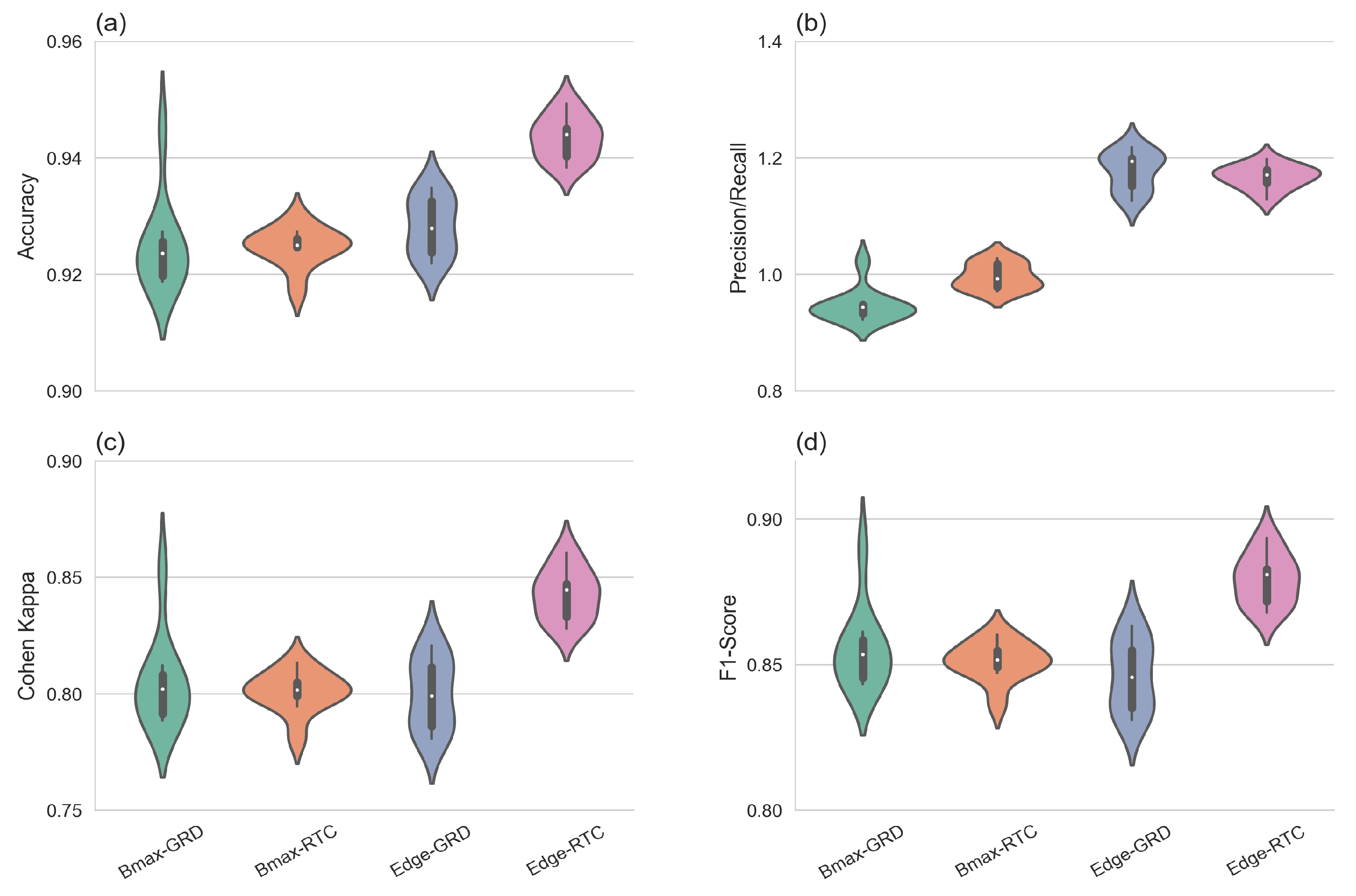
| Statistic | Bmax Otsu GRD | Bmax Otsu RTC | Edge Otsu GRD | Edge Otsu RTC |
|---|---|---|---|---|
| Overall Accuracy | 0.925 (0.007) | 0.925 (0.003) | 0.928 (0.005) | 0.943 (0.004) |
| Precision/Recall | 0.946 (0.028) | 0.996 (0.022) | 1.18 (0.033) | 1.17 (0.020) |
| Cohen Kappa | 0.804 (0.019) | 0.801 (0.009) | 0.800 (0.015) | 0.843 (0.011) |
| F1 Score | 0.855 (0.014) | 0.851 (0.007) | 0.846 (0.012) | 0.879 (0.009) |
| Bmax Otsu GRD | Bmax Otsu RTC | Edge Otsu GRD | |
|---|---|---|---|
| Bmax Otsu RTC | 1.0 | ||
| Edge Otsu GRD | 0.790 | 0.790 | |
| Edge Otsu RTC | 0.159 | 0.159 | 0.253 |
© 2020 by the authors. Licensee MDPI, Basel, Switzerland. This article is an open access article distributed under the terms and conditions of the Creative Commons Attribution (CC BY) license (http://creativecommons.org/licenses/by/4.0/).
Share and Cite
Markert, K.N.; Markert, A.M.; Mayer, T.; Nauman, C.; Haag, A.; Poortinga, A.; Bhandari, B.; Thwal, N.S.; Kunlamai, T.; Chishtie, F.; et al. Comparing Sentinel-1 Surface Water Mapping Algorithms and Radiometric Terrain Correction Processing in Southeast Asia Utilizing Google Earth Engine. Remote Sens. 2020, 12, 2469. https://0-doi-org.brum.beds.ac.uk/10.3390/rs12152469
Markert KN, Markert AM, Mayer T, Nauman C, Haag A, Poortinga A, Bhandari B, Thwal NS, Kunlamai T, Chishtie F, et al. Comparing Sentinel-1 Surface Water Mapping Algorithms and Radiometric Terrain Correction Processing in Southeast Asia Utilizing Google Earth Engine. Remote Sensing. 2020; 12(15):2469. https://0-doi-org.brum.beds.ac.uk/10.3390/rs12152469
Chicago/Turabian StyleMarkert, Kel N., Amanda M. Markert, Timothy Mayer, Claire Nauman, Arjen Haag, Ate Poortinga, Biplov Bhandari, Nyein Soe Thwal, Thannarot Kunlamai, Farrukh Chishtie, and et al. 2020. "Comparing Sentinel-1 Surface Water Mapping Algorithms and Radiometric Terrain Correction Processing in Southeast Asia Utilizing Google Earth Engine" Remote Sensing 12, no. 15: 2469. https://0-doi-org.brum.beds.ac.uk/10.3390/rs12152469