Article

Multi-Year Comparison of CO2 Concentration from NOAA Carbon Tracker Reanalysis Model with Data from GOSAT and OCO-2 over Asia

1
Collaborative Innovation Center on Forecast and Evaluation of Meteorological Disasters, Key Laboratory for Aerosol-Cloud-Precipitation of China Meteorological Administration, Key Laboratory of Meteorological Disasters, Ministry of Education, Nanjing University of Information Science and Technology, Nanjing 210044, China
2
School of Marine Sciences, Nanjing University of Information Science and Technology, Nanjing 210044, China
3
School of Atmospheric Sciences, Nanjing University of Information Science and Technology, Nanjing 210044, China
*
Author to whom correspondence should be addressed.
Remote Sens. 2020, 12(15), 2498; https://0-doi-org.brum.beds.ac.uk/10.3390/rs12152498
Submission received: 9 June 2020 / Revised: 28 July 2020 / Accepted: 3 August 2020 / Published: 4 August 2020
(This article belongs to the Special Issue Remote Sensing of Greenhouse Gases and Air Pollution)

Abstract

:
Accurate knowledge of the carbon budget on global and regional scales is critically important to design mitigation strategies aimed at stabilizing the atmospheric carbon dioxide (CO2) emissions. For a better understanding of CO2 variation trends over Asia, in this study, the column-averaged CO2 dry air mole fraction (XCO2) derived from the National Oceanic and Atmospheric Administration (NOAA) CarbonTracker (CT) was compared with that of Greenhouse Gases Observing Satellite (GOSAT) from September 2009 to August 2019 and with Orbiting Carbon Observatory 2 (OCO-2) from September 2014 until August 2019. Moreover, monthly averaged time-series and seasonal climatology comparisons were also performed separately over the five regions of Asia; i.e., Central Asia, East Asia, South Asia, Southeast Asia, and Western Asia. The results show that XCO2 from GOSAT is higher than the XCO2 simulated by CT by an amount of 0.61 ppm, whereas, OCO-2 XCO2 is lower than CT by 0.31 ppm on average, over Asia. The mean spatial correlations of 0.93 and 0.89 and average Root Mean Square Deviations (RMSDs) of 2.61 and 2.16 ppm were found between the CT and GOSAT, and CT and OCO-2, respectively, implying the existence of a good agreement between the CT and the other two satellites datasets. The spatial distribution of the datasets shows that the larger uncertainties exist over the southwest part of China. Over Asia, NOAA CT shows a good agreement with GOSAT and OCO-2 in terms of spatial distribution, monthly averaged time series, and seasonal climatology with small biases. These results suggest that CO2 can be used from either of the datasets to understand its role in the carbon budget, climate change, and air quality at regional to global scales.

Graphical Abstract

1. Introduction

Dealing with global climate change requires accurate knowledge of the global budget of atmospheric greenhouse gases [1]. Atmospheric carbon dioxide (CO2) is an important greenhouse gas that plays a significant role in several atmospheric phenomena such as hydrology, sea ice melting, sea level increasing and most importantly the temperature [2,3]. Since the industrial revolution, a notable increase in global CO2 concentration has been observed from 280 ppm in the middle of the 19th century to over 400 ppm to date [4,5,6]. Combustion of fossil fuel, land-use changes, and cement production are the major causes of increased CO2 concentration [7].
Asia, with the world’s 10 largest CO2 emitting nations, has become increasingly important in studying the global carbon budget. The poverty elimination efforts by the rapidly growing economies of the continent have largely relied on the construction of fossil-fuel based power and industrial projects which have significantly contributed to the greenhouse gases emissions [8]. Knowledge of regional contributions of CO2 is critically important to design mitigation strategies aimed at stabilizing the CO2 emissions. Much efforts have been made for estimating carbon sources and sinks in Asia, but still, they remain poorly quantified [9,10]. A detailed budget of CO2 exchange between the earth’s surface and the atmosphere is not available for some regions like South Asia, due to a sparse network of key carbon observations [11]. Moreover, Asia also remains one of the regions with large uncertainties in the carbon budget. In particular, the boreal and eastern part of Asia produces large uncertainties because of the large land surface heterogeneity and complex interactions between biosphere and atmosphere [12]. There is a need to expand the atmospheric observation network and develop inverse modelling systems for the effective use of in situ and remote sensing data streams [13].
A comprehensive network of ground-based, sun-viewing, near-IR, Fourier transform spectrometers known as Total Carbon Column Observing Network (TCCON) has been established to accurately measure the atmospheric greenhouse gases such as CO2, CO, N2O, and CH4 [14,15]. A significant effort has been applied and the CO2 measurements taken by TCCON have resulted in a precision of 0.25% under clear atmospheric conditions [16]. However, because of limited spatial coverage and uneven distribution of the TCCON sites, accurate CO2 amounts cannot be measured on sub-continental and regional spatial scales [17]. Studies suggest that the satellite observations, with their lower precision than the ground-based measurements but higher spatial coverage, can help to improve the CO2 measurements [18,19,20].
Over the past decade, multiple satellites such as the Greenhouse Gases Observing Satellite (GOSAT), Orbiting Carbon Observatory 2 (OCO-2) [21,22] and TanSat [23,24] have been dedicated to improving the CO2 measurements and covering the spatiotemporal gaps. GOSAT and OCO-2 have a common observational approach. For example, both the satellites have the solar reflectance spectra centered around 1.6 and 2.0 µm which are used to determine the CO2 optical depth and band A which is centered around 0.76 µm to measure the O2 optical depth. The information from these three spectral regions is combined to determine the XCO2 retrieval. XCO2 is a column-averaged CO2 dry air mole fraction that shows spatiotemporal variability and helps in improving the estimations of CO2 concentrations and constraining the model simulations by minimizing the uncertainties of CO2 sources and sinks. It has been shown that in the presence of optically thin clouds or aerosols, neglecting scattering can lead to unacceptably large retrieval errors [25]. Several retrieval algorithms, such as the National Institute of Environment Studies (NIES) XCO2 retrieval algorithm [26], University of Leicester full physics retrieval algorithm [27], and NASA’s Atmospheric CO2 Observations from Space (ACOS) XCO2 retrieval algorithm [28,29] have devised different approaches to deal with the scattering effects in the retrieval of the CO2. GOSAT contains the Clouds and Aerosol Imager (CAI) to detect the clouds but OCO-2 does not have any dedicated instrument to detect the clouds and aerosols. Although the satellite data are corrected (retrievals with the large error are screened out), uncertainties remain in the data. Therefore, the satellite datasets are validated against precise datasets to ensure the data quality and compared with the other datasets to assess the consistency and potential for joint utilization.
The CarbonTracker (CT), originally developed by National Oceanic and Atmospheric Administration (NOAA), is a modern data assimilation system that integrates the data into a consistent estimate of surface CO2 exchange [30]. CT incorporates daily CO2 measurements derived from the network of tall towers calibrated according to the world CO2 standard. Better knowledge and understanding of regional and global carbon cycles depend on the accuracy of the CO2 estimations. Therefore, the satellite and the model data need to be validated against other satellite observations and/or in situ observations before using them to answer scientific questions.
Many inter-comparisons and validation studies have reported discrepancies in regional and global carbon budgets and their spatial distributions because of differences in their set of criteria, approaches, assumptions, and accuracy of the available data. Because of quality control purposes, much of the space-based observations are screened out during pre-processing. Oshchepkov et al. [31] pointed out that less than 10% of the total measurements become usable after retrieval and the screening processing. This might be due to the high amount of aerosol which significantly limits XCO2 coverage. Deng et al. [32] compared the NIES and ACOS retrieval algorithms results for GOSAT with the TCCON site and reported the overall bias of 0.21 ± 1.85 ppm and −0.69 ± 2.13 ppm for ACOS and NIES XCO2, respectively. Moreover, the greatest monthly mean difference of 1.43 ± 0.60 ppm lies over China. Jing et al. [33] compared the CO2 concentration simulated by GEOS-Chem with GOSAT, CT, and TCCON. GEOS-Chem is overestimated by an amount of 0.78 ppm when compared with GOSAT, slightly underestimated when compared with the CT, and underestimated by an amount of 1 ppm when compared with the TCCON. Kulawik et al. [34] compared the multiple CO2 data sources with the TCCON and found mean root square deviations of 1.7 and 0.9 in GOSAT and CT2013x XCO2 retrievals, respectively. These findings suggest that there is an imminent need to assess the accuracy and uncertainty of XCO2 observations derived from the space-based data against in-situ measurements and accurate simulations by models. Moreover, the inter-comparisons between the models and other CO2 data sources are also essential to quantitatively evaluate the model uncertainties and further improve the results.
This study aims to inter-compare the CT CO2 characteristics with ACOS/GOSAT and OCO-2 XCO2 retrievals over Asia and separately on its five regions i.e., Central Asia, East Asia, South Asia, Southeast Asia, and Western Asia from September 2009 to August 2019. Furthermore, the ability and consistency of the CarbonTracker to capture the seasonal and inter-annual variations of CO2 amplitude over different regions of Asia have been assessed.

2. Materials and Methods
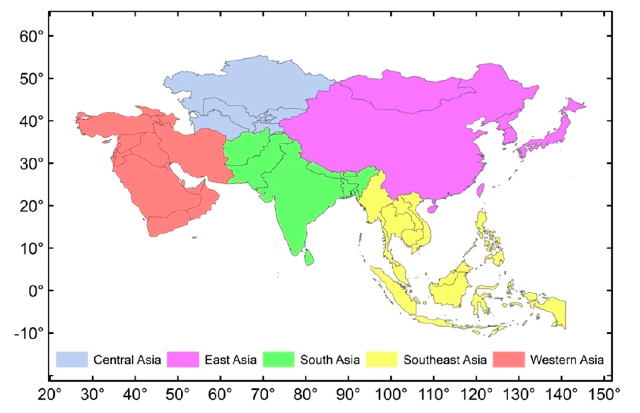
2.1. Study Area

Asia covers one-third of the Earth’s surface and almost every known climate occurs on this continent [35]. The climatic heterogeneity in Asia is driven by several factors such as humidity, temperature, precipitation, spatial distribution and intensity of solar energy, wind pattern and atmospheric pressure. CO2 fluxes observe seasonal variability and to determine the regional variability, Asia has been divided into five regions (Figure 1). The region names and the countries are given in the following:
This study is carried out over Asia as a whole and separately in each of its regions, given in Table 1.

2.2. Datasets

2.2.1. GOSAT Observations

GOSAT, the world’s first satellite dedicated to measuring the concentrations of CO2 and CH4 from space, is a joint venture of Japan Aerospace Exploration Agency (JAXA), NIES, and Ministry of Environment (MOE). GOSAT was launched on 23 January 2009 and it takes measurements of reflected sunlight in three near-infrared bands with a circular footprint of approximately 10.5 km diameter at the nadir [29,36,37]. It incorporates two instruments: the Thermal and Near-infrared Sensor for carbon Observation-Fourier Transform Spectrometer (TANSO-FTS), and the Thermal and Near-infrared Sensor for carbon Observation-Cloud and Aerosol Imager (TANSO-CAI). TANSO-FTS is responsible for measuring the greenhouse gases with three narrow SWIR bands (0.76, 1.6 and 2.0 µm) and a wide thermal band (5.5–14.3 µm) at a spectral resolution of 0.2−1 cm. The SWIR bands are mainly responsible for retrieving CO2 column concentrations while the TIR band retrieves the vertical profiles of CO2 concentrations [38]. Clouds and aerosols strongly affect the quality of CO2 observations [39]. TANSO-CAI retrieves the cloud and aerosol information [40,41]. In this study, the ACOS/GOSAT XCO2 version 9.3 Level 2 Lite product has been used [16,28,29]. ACOS/GOSAT XCO2 has lower bias and better consistency compared to NIES/GOSAT [32].

2.2.2. OCO-2 Observations

NASA’s Orbiting Carbon Observatory-2 is the second satellite after GOSAT dedicated to monitoring atmospheric CO2 to obtain better knowledge and understanding of the carbon cycle. The main objectives of the mission include measuring CO2 with enough precision, accuracy, and spatial and temporal resolutions required to quantify the CO2 sources and sinks at regional and global levels. The sun-synchronous, near-polar satellite incorporates three high-resolution spectrometers making coincident measurements of reflected sunlight in the near-infrared CO2 near 1.61 and 2.06 µm and molecular oxygen (O2) A-Band at 0.76 µm with a temporal resolution of 16 days allowing the complete global coverage of XCO2 twice per month [27,42,43,44]. In this study, OCO-2 XCO2 version 9r Level 2 Lite product has been used. These data were produced by OCO-2 project at the Jet Propulsion Laboratory, California Institute of Technology, and obtained from OCO-2 data archive maintained at the NASA Goddard Earth Science Data and Information Services Center.

2.2.3. CarbonTracker Measurements

CarbonTracker (CT), developed by Peters et al. [45,46], is an inverse modelling framework that updates the atmospheric CO2 distribution and the surface fluxes annually. It incorporates the two-way nested Transport Model 5 (TM5) offline atmospheric tracer transport model which supports high-resolution data regionally and coarse resolution data globally [47]. CT forecasts the CO2 mole fraction by combing CO2 surface exchange models and TM5 model driven by the meteorology from the European Center for Medium-Range Weather Forecasts (ECMRWF) ERA-interim reanalysis [48]. The resulting three-dimensional CO2 distribution is then sampled at the time and location that observations are available, and the difference between observations and model forecasts is minimized [30]. The CT provides the global CO2 distribution at 25 pressure levels with the spatial resolution of 3° × 2° Longitude/Latitude and temporal resolution of 3 h.
In this study, we have used CT2019 release and near real-time version (CT19NRT20). Previous versions of the modelled data have been compared with other CO2 data sources and results suggest that CT captures the XCO2 reasonably well. More detail about CT data can be accessed at (https://www.esrl.noaa.gov/gmd/ccgg/CT/).

2.3. Methods

Different CO2 data products cannot be compared directly because of their differences in sampling methods and data sources. For instance, CO2 products retrieved from OCO-2 and GOSAT are CO2 column-averaged dry air mole fraction (XCO2) concentrations while the simulated results from the CarbonTracker are CO2 profiles with 25 vertical profiles. Moreover, the CT model gives well distributed smooth data with a temporal resolution of 3 h and a spatial resolution of 3° × 2° Longitude/Latitude, while the satellite observations are different in terms of time and space. In satellite data, the screening process and cloud filtering significantly reduce the data quantity, which consequently produces gaps. In addition, the temporal resolution also contributes to mismatching between the model and the satellite data. As a result, both of the datasets cannot be compared directly because there is no match between the two datasets in terms of spatial and temporal resolutions. Thus, the CT mole fraction of CO2 is extracted on the time and location of the satellite data. By keeping the grid points of CT as standard, the corresponding XCO2 from the satellite observations are extracted for a spatial window of 1.5° × 1.5° with their centers at the reference grid points of the CT. Furthermore, to make both the datasets comparable, it is mandatory to adjust the vertical resolutions of the datasets accordingly. To deal with the different number of vertical levels of both datasets, CT CO2 is interpolated to the vertical numbers of the satellite datasets. The CT XCO2 ( XCO 2 m ), that is used to compare with the satellite datasets is computed by the procedure as suggested by [33,49,50].
XCO 2 m = XCO 2 a + j p j T K j ( CO 2 i CO 2 a ) ,
where, ( XCO 2 a ) is XCO 2 a priori, (p) is pressure weighting function, (K) is an averaging kernel, ( CO 2 i ) is interpolating CT CO2, ( CO 2 a ) is a priori profile, (j) refers to satellite retrieval vertical level, and (T) indicates the matrix transpose. Some other statistical calculations such as correlation coefficients (R), and Root Mean Square Deviation (RMSD) have also been computed to determine the level of agreement between the CT and respective satellite datasets. The correlation coefficient for the jth pixel is computed by the formula given:
R j = 1 n i = 1 n ( M i M ¯ ) ( 1 n i = 1 n ( S i S ¯ ) , 1 n i = 1 n ( M i M ¯ ) 2 1 n i = 1 n ( S i S ¯ ) 2
where ( M ¯ ) and ( S ¯ ) represent the mean values of CT and satellite XCO2 retrievals. The RMSD showing the standard error of the model against the observations at the jth pixel is calculated as follows:
RMSD j = 1 n i = 1 n ( ( M i M ¯ ) ( S i S ¯ ) ) 2
More detail about the Root Mean Squared Deviation (RMSD) is given in [51].

3. Results and Discussion

3.1. Comparison of NOAA CarbonTracker with GOSAT and OCO-2

NOAA CarbonTracker has been compared with ACOS/GOSAT version 9.3 and OCO-2 version 9r for durations of 10 years starting from September 2009 to August 2019 and 5 years ranging from September 2014 to August 2019, respectively. The CT dataset is made comparable with the satellite datasets following the procedure described in Section 2.2 The results are based on 519 points which are uniformly distributed over Asia with a spatial resolution of 3° × 2° Longitude/Latitude.
Figure 2 shows the distribution of 10 years averaged XCO2 over Asia for CT (Figure 2a) and GOSAT (Figure 2b). The number of datasets used in the analysis is shown in Figure 2d. The datasets in each grid range from 11 to 2239. The comparison shows that the spatial distribution characteristics are consistent between both of the datasets with a spatial mean correlation of 0.93.
Figure 3 shows the distribution of temporally averaged XCO2 derived from the CT (Figure 3a) and OCO-2 (Figure 3b) over Asia for 5 years ranging from September 2014 to August 2019. Southeast Asia and some parts of China observe the least number of cloud-free observations from OCO-2 (Figure 3d). The two datasets show good consistency with a spatial mean correlation of 0.89. OCO-2 has better spatial coverage than GOSAT over Asia (Figure 2d and Figure 3d), however, both show a small number of retrievals over East Asia and Southeast Asia. This may be due to the ACOS XCO2 retrieval algorithm which excludes the data with high aerosol optical depth and cloud optical thickness [28,29] and results in reducing XCO2 data quantity over Asian regions during the monsoon [52] and high pollution events, which typically occur in the spring [53]. Both the model and the satellite datasets observe the highest CO2 emission over high density urban regions such as Beijing-Tianjin-Hebei area in northern China, Korea and Japan (Figure 2a,b and Figure 3a,b). These are the most populated regions with the largest anthropogenic emissions in the world [54,55]. The distribution characteristics of XCO2 values retrieved from GOSAT and OCO-2 are similar to the modelled XCO2 over most of the regions except some parts of East Asia such as China and Mongolia (Figure 2c and Figure 3c). GOSAT dataset shows a higher standard deviation compared to OCO-2, and these results are supported by a previous study which has also reported a large standard deviation of GOSAT observations compared to OCO-2 at the TCCON sites [56]. The differences over China maybe mostly attributed to the large uncertainties in the terrestrial flux estimation as previous studies have reported poor performance of terrestrial flux from CT2015 against in situ observations obtained from eight sites of the Chinese Terrestrial Ecosystem Flux Observation and Research Network (ChinaFLUX) [57,58,59,60]. The substantial difference exists over the Qinghai Tibet Plateau, which is the highest terrain of the earth located in the southwest of China. The CT shows higher XCO2 concentrations over mountain ranges of northern Mongolia, northern Afghanistan, Tajikistan and Kyrgyzstan compared to OCO-2 (Figure 3c). Kong et al. [56] also found significantly larger values of the CarbonTracker XCO2 over Tibetan Plateau and mountain ranges compared to those of the satellite datasets.
Compared to the satellite datasets, CT is overestimated by −0.61 ± 0.96 ppm against GOSAT and underestimated by 0.31 ± 0.71 ppm against OCO-2 over Asia. Furthermore, the summaries of both comparisons including the regional detail are given in Table 2 and Table 3.
As a one-to-one comparison between CT model data and the satellite observations is not possible, it is therefore important to determine the relative spatial distance between the occurrences of both datasets. The satellite values are averaged in a 1.5° × 1.5° window centering the grid cell of CT. The spatial distance means a distance between a given GOSAT/OCO-2 measurement and CT grid point.
Figure 4 shows the scatter density plot between the CT and GOSAT (Figure 4a) and CT and OCO-2 (Figure 4b) XCO2 concentrations. The color represents the relative spatial distance between the points of CT and the satellite datasets in terms of degree. The spatial distance between the points represents the spatial mismatch and does not indicate differences between the XCO2 values of the datasets.
Figure 5 shows the spatial distribution of the correlations between the model and the satellite datasets. The results show a good correlation between CT and GOSAT (Figure 5a), and between CT and OCO-2 (Figure 5b) over Asia except for East Asia. However, a low correlation (<0.4) between CT and GOSAT is observed only over southwest China, while a low correlation (<0.4) between CT and OCO-2 is observed over southwest China, the northern part of Pakistan, northern Afghanistan, Tajikistan and Kyrgyzstan. These regions are either the plateaus or the mountain ranges. Both the model and the satellite datasets contribute to the uncertainties. Connor et al. [50] presented the OCO inverse method and prospective error analysis and concluded that the instrument can produce the single sounding error up to 0.8 ppm for sun conditions and up to 2.5 ppm for low sun conditions over the low- and mid-latitudes due to noise, geophysical and spectroscopic errors. To determine if it is the model data which originates the error or whether satellite data also contributes to it, the spatial distribution of the posterior XCO2 error for GOSAT and OCO-2 is also shown in Figure 5c,d, respectively. The posterior XCO2 error is computed by combing interference errors, smoothing errors and instrument noise [50]. GOSAT posterior XCO2 error is larger than that of OCO-2 and it becomes significant from East China to West China.
In general, the CT-GOSAT comparison implies that both of the datasets are characterized by a high spatial mean correlation of 0.93, a global offset of −0.61 ppm, which suggests that CT XCO2 is lower relative to that of GOSAT, RMSD of 2.61 ppm and relative accuracy of 0.96 ppm over Asia. The comparison between the CT and OCO-2 shows CT is overestimated by an amount of 0.31 ppm and exhibits a spatial mean correlation of 0.89, RMSD of 2.16 ppm and relative accuracy of 0.71 ppm. Furthermore, the summaries of both comparisons including the regional detail are given in Table 2 and Table 3.

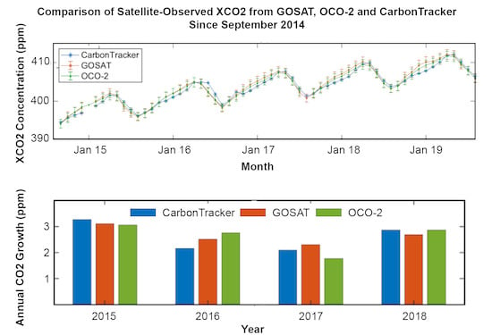
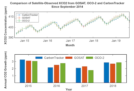
3.1.1. Monthly Averaged Time-Series Comparison

Figure 6 shows the monthly averaged XCO2 variations from CT and the two satellite datasets for 5 years starting from September 2014 to August 2019 over Asia (Figure 6a), Central Asia (Figure 6b), East Asia (Figure 6c), South Asia (Figure 6d), Southeast Asia (Figure 6e), and Western Asia (Figure 6f). All the data products show similarity in phases and amplitudes with some differences in the magnitude, which suggests a good agreement between the model and the satellite datasets. The CO2 concentrations over Central Asia (Figure 6b), East Asia (Figure 6c), and Southeast Asia (Figure 6e) are the highest in April and the lowest in August. It starts increasing in the fall, continues to increase in the winter, and reaches the maximum value in spring. In these regions, the heating systems are used in winter and spring which consume larger amounts of fossil energy, such as natural gas, oil, and coal, and thus produce a large amount of the CO2 which is discharged into the atmosphere. Moreover, in winter and spring, the plants are in the dormant and recovery stage. During this period, the strong respiration and the weak photosynthesis also contribute significantly to increasing the CO2 concentration in the atmosphere. The lower temperature in the winter inhibits the microorganism activity which hinders the decomposition process. The temperature starts increasing in the late spring, and it enhances the microorganism activity, thus the decomposition is started and CO2 is released from the biological materials. This might be the reason for the maximum concentration of the CO2 in April. The CO2 concentration decreases from May to August. During this period, the temperature, precipitation, and the lightning are beneficial to the vegetation growth which enhances the photosynthesis process. The strong presence of the photosynthesis by vegetation decays CO2 concentration [61,62]. Compared to the CT, GOSAT and OCO-2 show lower CO2 concentrations during the wet season (April-August) over these regions.
Asia experiences a monsoon climate, which plays a significant role in the CO2 concentrations [63]. Asian monsoon may be further classified into the Southwest Monsoon and the East Asian Monsoon [64]. The Southwest Monsoon mostly affects the Indian subcontinent and the East Asian Monsoon affects China, Japan, Philippines, Korea and Taiwan. The occurrence of the summer monsoons is a major source of precipitation and thus an important factor controlling the vegetation in these regions. Generally, March to May is treated as pre-monsoon, June to September as monsoon and October to November as post-monsoon in most of the Asian regions [63]. The CO2 concentration is found to be maximum in the pre-monsoon and minimum in monsoon (Figure 6c,d).
The highest CO2 concentration in the pre-monsoon maybe due to the higher temperature and solar radiation prevailing during these months, which stimulate the assimilation of CO2 in the daytime and respiration in the night [65]. The low wind speed during the pre-monsoon causes slight mixing in the boundary layer which also contributes in the CO2 concentration [66]. Moreover, a large amount of biomass burning and forest fires during this period also compliment the increase in CO2 concentration [67,68]. The reduction in CO2 concentration in monsoon is maybe because of the monsoon precipitation resulting in increasing the soil moisture which enhances the photosynthesis process. Moreover, the presence of clouds during the season decreases the temperature which reduces the leaf and soil respiration rate which eventually increases the carbon uptake [68]. The CO2 starts increasing in post-monsoon which is associated with microbial activity and high ecosystem productivity [66,69]. The fluctuations in the CT XCO2 have been observed during this season over East Asia and South Asia. Moreover, the CT shows higher CO2 concentration compared to GOSAT and OCO-2 during monsoon (Table 4 and Table 5). The higher CO2 concentration over monsoon-affected regions might be due to the uncertainties involved in realizing the inversion during the monsoon season, in the presence of clouds [70].
The monthly averaged statistical relationships between the CT and satellite datasets are given in Table 6 and Table 7. The CT is underestimated over all the regions of Asia when compared with GOSAT and overestimated over all the regions except East Asia when compared with OCO-2. East Asia exhibits lower correlation and higher RMSD values relative to other regions. The CT shows smaller RMSD with OCO-2 compared to GOSAT.
Figure 7 shows the annual growth of XCO2 derived from the model and the two satellite datasets over Asia, Central Asia, East Asia, South Asia, Southeast Asia, and Western Asia.
The annual growth rate has been computed by subtracting the mean from the mean of the next year. The annual growth of CO2 rate ranges from 0.98 to 3.28 ppm. It is important to note that in all the data products, the annual growth rate is relatively higher in 2015. This is because of 2015 El Niño which occurred in March 2015. El Niño–Southern Oscillation (ENSO), characterized by anomalous sea surface warming and cooling in the eastern and central Pacific is closely related to the growth rate of atmospheric CO2 [71]. Atmospheric CO2 growth rate is increased during El Niño and decreases during La Nina [72]. The computed growth rates are in agreement with the NOAA growth rates from CO2 surface observations [5] and the World Data Center for Greenhouse Gases (WDCGG) (https://gaw.kishou.go.jp/publications/global_mean_mole_fractions).

3.1.2. Seasonal Climatology Comparison

Figure 8 shows the seasonal variations of XCO2 derived from the CT and GOSAT over Asia for a period of 10 years staring from September 2009 to August 2019 for four seasons based on the three months; winter (December January February or DJF), spring (March April May or MAM), summer (June July August or JJA) and autumn (September October November or SON). The seasonal cycle has significant effects on CO2 concentration.
The higher CO2 concentrations have been observed in winter and spring while the lower ones occurred in summer and autumn. This trend is common in the Northern Hemisphere [33]. The weak photosynthesis, microorganism activity, and the heating measures are the major causes of the increased CO2 concentrations in winter and the spring; while CO2 uptake from vegetation in summer removes CO2 from the atmosphere and decreases the CO2 concentrations. In winter, spring, and autumn, the CT XCO2 is smaller than that of GOSAT (Figure 8). During winter, the difference between the two datasets is significant and it reaches over −2 ppm in western China and the western part of Central Asia. Kog et al. [56] compared the seasonal climatology of CT2017 with GOSAT and found that the differences in most of the regions were within ±2.5 ppm. In the summer, the CT shows higher CO2 concentrations relative to GOSAT. It is important to note that during this season, the monsoon is active in Asian regions. Nalini et al. [70] also found that the CT shows higher concentrations over Indian regions during the monsoon. More detail about seasonal climatology comparison between the two datasets over Asian regions is given in the Table 8.
Figure 9 shows the spatial distribution of seasonal averaged XCO2 from the CT (left panel), OCO-2 (middle panel), and their differences (right panel) over Asia for a period of 5 years ranging from September 2014 to August 2019. Spatial distribution characteristics are consistent between CT and OCO-2. XCO2 increases from winter (DJF) to spring (MAM), with the highest concentration observed during spring and decreases from summer (JJA) to autumn (SON), with the lowest concentration during SON. The decreasing trend from MAM to JJA to SON has likely resulted from the vegetation awakening as the photosynthesis from the vegetation leads to decaying of the CO2 concentration. The decay of vegetation in autumn and the heating measures in winter result in increasing the CO2 concentration. Figure 9 (right panel) displays the seasonal mean differences of XCO2 from the two datasets. Both of the datasets show good agreement with each other. In most of the regions of the continent, the mean seasonal difference ranges from −1 to +1 ppm. East Asia is the region with the highest uncertainties in the continent. The highest mean difference (>2 ppm) and the lowest mean difference (<−2 ppm) have been observed in summer (JJA) and autumn (SON), respectively, over East Asia. This indicates that CT produces higher XCO2 concentration when the vegetation cover decreases and produces the opposite when the vegetation cover is strong relative to OCO-2. The CT is overestimated during all the seasons over Asia when compared with OCO-2. More detail about seasonal climatology comparison between CT and OCO-2 datasets is given in the Table 9.

4. Conclusions

This study compared the NOAA CT XCO2 with that of GOSAT and OCO-2. Comparison between the CT and GOSAT has been achieved using 10 years of data ranging from September 2009 to August 2019 and the comparison between the CT and OCO-2 has been performed using 5 years of data starting from September 2014 to August 2019.
The results found that the CT XCO2 is underestimated by 0.61 ppm when compared with GOSAT and overestimated by 0.31 ppm when compared with OCO-2. The differences between CT and OCO-2 are within ±1.0 ppm over most of the regions, while CT and GOSAT differ greatly as the differences between the CT and GOSAT are within ±2.0 ppm over most of the regions. Comparison between CT and satellite datasets (GOSAT and OCO-2) showed larger differences over China which may be attributed to the greater uncertainties in model terrestrial flux. The CT shows higher CO2 concentrations compared to GOSAT and OCO-2 over the Tibet Plateau and the other mountain ranges.
The monthly time-series showed an agreement between CT and both GOSAT and OCO-2 in terms of amplitude and pattern. However, this agreement deteriorates over South Asia and East Asia during monsoon. The CT also showed higher XCO2 concentrations and more fluctuations during the monsoon when compared with the XCO2 retrieved from GOSAT and OCO-2. In the seasonal climatology comparison, the CT XCO2 is more than that of OCO-2 during all the seasons whereas, the CT shows lower XCO2 concentrations during autumn, winter, and spring when compared with GOSAT. The seasonal climatology between and model and the satellite datasets shows that the CT has the ability to capture the seasonal cycle.
The model and the satellite datasets have a good agreement in terms of the spatial distribution, monthly averaged distribution and seasonal climatology. These results suggest that CO2 can be used from either of the datasets to understand its role in the carbon budget at a regional scale. The large uncertainties in East Asia, in particular, China are challenging. The land-use activities such as deforestation and intense agriculture also affect the CO2 concentrations. Moreover, recent studies have suggested that current aerosol loading over China may affect the terrestrial carbon fluxes as well as the atmospheric CO2 concentrations by diffuse radiation fertilization effects and hydrometeorological feedbacks. These effects also need to be considered in future studies.

Author Contributions

Formal analysis, Q.W.; Methodology, F.M.; Supervision, L.B.; Writing–review & editing, M.A.A., M.B., M.S. and Z.Q. All authors have read and agreed to the published version of the manuscript.

Funding

This research was funded by National Natural Science Foundation of China (NSFC), grant number 41675133 and the Special Project of Jiangsu Distinguished Professor, grant number (1421061901001) by Jiangsu Provincial Department of Education.

Acknowledgments

The authors acknowledge the efforts of NASA to provide the OCO-2 data products. These data were produced by the OCO-2 project at the Jet Propulsion Laboratory, California Institute of Technology, and obtained from the OCO-2 data archive maintained at the NASA Goddard Earth Science Data and Information Services Center. The authors also acknowledge NOAA Earth System Research Laboratory for their data products. The foremost author (Farhan Mustafa) is thankful to Anteneh Getachew for his support. The foremost author (Farhan Mustafa) and the 4th author (Md. Arfan Ali) are highly grateful to the China Scholarship Council (CSC) and the NUIST for granting the fellowship and providing the required supports.

Conflicts of Interest

The authors declare no conflict of interest.

References

  1. Umezawa, T.; Matsueda, H.; Sawa, Y.; Niwa, Y.; Machida, T.; Zhou, L. Seasonal evaluation of tropospheric CO2 over the Asia-Pacific region observed by the CONTRAIL commercial airliner measurements. Atmos. Chem. Phys. 2018, 18, 14851–14866. [Google Scholar] [CrossRef] [Green Version]
  2. Santer, B.D.; Painter, J.F.; Bonfils, C.; Mears, C.A.; Solomon, S.; Wigley, T.M.L.; Gleckler, P.J.; Schmidt, G.A.; Doutriaux, C.; Gillett, N.P.; et al. Human and natural influences on the changing thermal structure of the atmosphere. Proc. Natl. Acad. Sci. USA 2013, 110, 17235–17240. [Google Scholar] [CrossRef] [PubMed] [Green Version]
  3. Stocker, B.D.; Roth, R.; Joos, F.; Spahni, R.; Steinacher, M.; Zaehle, S.; Bouwman, L.; Xu-Ri; Prentice, I.C. Multiple greenhouse-gas feedbacks from the land biosphere under future climate change scenarios. Nat. Clim. Chang. 2013, 3, 666–672. [Google Scholar] [CrossRef]
  4. Ballantyne, A.P.; Alden, C.B.; Miller, J.B.; Trans, P.P.; White, J.W.C. Increase in observed net carbon dioxide uptake by land and oceans during the past 50 years. Nature 2012, 488, 70–73. [Google Scholar] [CrossRef]
  5. Dlugokencky, T.P. (Ed.) Trends in Atmospheric Carbon Dioxide. Available online: Ftp://aftp.cmdl.noaa.gov/products/trends/co2/co2_mm_gl.txt (accessed on 3 May 2020).
  6. Were, D.; Kansiime, F.; Fetahi, T.; Cooper, A.; Jjuuko, C. Carbon Sequestration by Wetlands: A Critical Review of Enhancement Measures for Climate Change Mitigation. Earth Syst. Environ. 2019, 3, 327–340. [Google Scholar] [CrossRef]
  7. Keeling, C.D.; Piper, S.C.; Heimann, M. A three-dimensional model of atmospheric CO2 transport based on observed winds: 4. Mean annual gradients and interannual variations. ASP Clim. Var. Pacific West. Am. 1989, 55, 305–363. [Google Scholar]
  8. Khalil, A.; Javed, A.; Bashir, H. Evaluation of Carbon Emission Reduction via GCIP Projects: Creating a Better Future for Pakistan. Earth Syst. Environ. 2019, 3, 19–28. [Google Scholar] [CrossRef]
  9. Zhang, H.F.; Chen, B.Z.; Machida, T.; Matsueda, H.; Sawa, Y.; Fukuyama, Y. Estimating Asian terrestrial carbon fluxes from CONTRAIL aircraft and surface CO 2 observations for the period 2006–2010. Atmos. Chem. Phys. 2014, 1, 5807–5824. [Google Scholar] [CrossRef] [Green Version]
  10. Pan, Y.; Birdsey, R.A.; Fang, J.; Houghton, R.; Kauppi, P.E.; Kurz, W.A.; Phillips, O.L.; Shvidenko, A.; Lewis, S.L.; Canadell, J.G.; et al. A Large and Persistent Carbon Sink in the World’s Forests. Science 2011, 333, 988–993. [Google Scholar] [CrossRef] [Green Version]
  11. Patra, P.K.; Canadell, J.G.; Houghton, R.A.; Piao, S.L.; Oh, N.H.; Ciais, P.; Manjunath, K.R.; Chhabra, A.; Wang, T.; Bhattacharya, T.; et al. The carbon budget of South Asia. Biogeosciences 2013, 10, 513–527. [Google Scholar] [CrossRef] [Green Version]
  12. Thompson, R.L.; Patra, P.K.; Chevallier, F.; Maksyutov, S.; Law, R.M.; Ziehn, T.; Van Der Laan-Luijkx, I.T.; Peters, W.; Ganshin, A.; Zhuravlev, R.; et al. Top-down assessment of the Asian carbon budget since the mid 1990s. Nat. Commun. 2016, 7, 1–10. [Google Scholar] [CrossRef] [PubMed] [Green Version]
  13. Patra, P.K.; Canadell, J.G.; Lal, S. The rapidly changing greenhouse gas budget of Asia. EOS Trans. Am. Geophys. Union 2012, 93, 237. [Google Scholar] [CrossRef]
  14. Toon, G.; Blavier, J.-F.; Washenfelder, R.; Wunch, D.; Keppel-Aleks, G.; Wennberg, P.; Connor, B.; Sherlock, V.; Griffith, D.; Deutscher, N.; et al. Total Column Carbon Observing Network (TCCON). In Proceedings of the Advances in Imaging; Optical Society of America: Washington, DC, USA, 2009; p. JMA3. [Google Scholar]
  15. Wunch, D.; Toon, G.C.; Wennberg, P.O.; Wofsy, S.C.; Stephens, B.B.; Fischer, M.L.; Uchino, O.; Abshire, J.B.; Bernath, P.; Biraud, S.C.; et al. Calibration of the total carbon column observing network using aircraft profile data. Atmos. Meas. Tech. 2010, 3, 1351–1362. [Google Scholar] [CrossRef] [Green Version]
  16. Wunch, D.; Wennberg, P.O.; Toon, G.C.; Connor, B.J.; Fisher, B.; Osterman, G.B.; Frankenberg, C.; Mandrake, L.; O’Dell, C.; Ahonen, P.; et al. A method for evaluating bias in global measurements of CO 2 total columns from space. Atmos. Chem. Phys. 2011, 11, 12317–12337. [Google Scholar] [CrossRef] [Green Version]
  17. Velazco, V.; Morino, I.; Uchino, O.; Deutscher, N.; Bukosa, B.; Belikov, D.; Oishi, Y.; Nakajima, T.; Macatangay, R.; Nakatsuru, T.; et al. Total Carbon Column Observing Network Philippines: Toward Quantifying Atmospheric Carbon in Southeast Asia. Clim. Disaster Dev. J. 2017, 2, 1–12. [Google Scholar] [CrossRef]
  18. Hungershoefer, K.; Peylin, P.; Chevallier, F.; Rayner, P.; Klonecki, A.; Houweling, S.; Marshall, J. Evaluation of various observing systems for the global monitoring of CO2 surface fluxes. Atmos. Chem. Phys. 2010, 10, 10503–10520. [Google Scholar] [CrossRef] [Green Version]
  19. Baker, D.F.; Bösch, H.; Doney, S.C.; O’Brien, D.; Schimel, D.S. Carbon source/sink information provided by column CO2 measurements from the Orbiting Carbon Observatory. Atmos. Chem. Phys. 2010, 10, 4145–4165. [Google Scholar] [CrossRef] [Green Version]
  20. Wang, H.; Jiang, F.; Wang, J.; Ju, W.; Chen, J.M. Differences of the inverted terrestrial ecosystem carbon flux between using GOSAT and OCO-2 XCO2 retrievals. Atmos. Chem. Phys. Discuss. 2018, 19, 1–32. [Google Scholar] [CrossRef]
  21. Crisp, D.; Miller, C.E.; DeCola, P.L. NASA Orbiting Carbon Observatory: Measuring the column averaged carbon dioxide mole fraction from space. J. Appl. Remote Sens. 2008, 2, 1–14. [Google Scholar] [CrossRef]
  22. Crisp, D. Measuring atmospheric carbon dioxide from space with the Orbiting Carbon Observatory-2 (OCO-2). In Earth Observing Systems; International Society for Optics and Photonics: Washington, DC, USA, 2015; Volume 9607. [Google Scholar]
  23. Wang, X.; Guo, Z.; Huang, Y.; Fan, H.; Li, W. A cloud detection scheme for the Chinese Carbon Dioxide Observation Satellite (TANSAT). Adv. Atmos. Sci. 2017, 34, 16–25. [Google Scholar] [CrossRef] [Green Version]
  24. Yang, D.; Liu, Y.; Cai, Z.; Chen, X.; Yao, L.; Lu, D. First Global Carbon Dioxide Maps Produced from TanSat Measurements. Adv. Atmos. Sci. 2018, 35, 621–623. [Google Scholar] [CrossRef]
  25. Kiel, M.; Dell, C.W.O.; Fisher, B.; Eldering, A.; Nassar, R.; Macdonald, C.G.; Wennberg, P.O. How bias correction goes wrong: Measurement of X CO 2 affected by erroneous surface pressure estimates. Atmos. Meas. Tech. 2019, 12, 2241–2259. [Google Scholar] [CrossRef] [Green Version]
  26. Yoshida, Y.; Ota, Y.; Eguchi, N.; Kikuchi, N.; Nobuta, K.; Tran, H.; Morino, I.; Yokota, T. Retrieval algorithm for CO 2 and CH 4 column abundances from short-wavelength infrared spectral observations by the Greenhouse gases observing satellite. Atmos. Meas. Tech. 2011, 4, 717–734. [Google Scholar] [CrossRef] [Green Version]
  27. Boesch, H.; Baker, D.; Connor, B.; Crisp, D.; Miller, C. Global characterization of CO2 column retrievals from shortwave-infrared satellite observations of the Orbiting Carbon Observatory-2 mission. Remote Sens. 2011, 3, 270–304. [Google Scholar] [CrossRef] [Green Version]
  28. O’Dell, C.W.; Connor, B.; Bösch, H.; O’Brien, D.; Frankenberg, C.; Castano, R.; Christi, M.; Eldering, D.; Fisher, B.; Gunson, M.; et al. The ACOS CO2 retrieval algorithm-Part 1: Description and validation against synthetic observations. Atmos. Meas. Tech. 2012, 5, 99–121. [Google Scholar] [CrossRef] [Green Version]
  29. Crisp, D.; Fisher, B.M.; O’Dell, C.; Frankenberg, C.; Basilio, R.; Bösch, H.; Brown, L.R.; Castano, R.; Connor, B.; Deutscher, N.M.; et al. The ACOS CO 2 retrieval algorithm-Part II: Global X CO2 data characterization. Atmos. Meas. Tech. 2012, 5, 687–707. [Google Scholar] [CrossRef] [Green Version]
  30. Peters, W.; Jacobson, A.R.; Sweeney, C.; Andrews, A.E.; Conway, T.J.; Masarie, K.; Miller, J.B.; Bruhwiler, L.M.P.; Pétron, G.; Hirsch, A.I.; et al. An atmospheric perspective on North American carbon dioxide exchange: CarbonTracker. Proc. Natl. Acad. Sci. USA 2007, 104, 18925–18930. [Google Scholar] [CrossRef] [PubMed] [Green Version]
  31. Oshchepkov, S.; Bril, A.; Yokota, T.; Morino, I.; Yoshida, Y.; Matsunaga, T.; Belikov, D.; Wunch, D.; Wennberg, P.; Toon, G.; et al. Effects of atmospheric light scattering on spectroscopic observations of greenhouse gases from space: Validation of PPDF-based CO2 retrievals from GOSAT. J. Geophys. Res. Atmos. 2012, 117, 1493–1512. [Google Scholar] [CrossRef] [Green Version]
  32. Deng, A.; Yu, T.; Cheng, T.; Gu, X.; Zheng, F.; Guo, H. Intercomparison of Carbon Dioxide Products Retrieved from GOSAT Short-Wavelength Infrared Spectra for Three Years (2010-2012). Atmosphere 2016, 7, 109. [Google Scholar] [CrossRef] [Green Version]
  33. Jing, Y.; Wang, T.; Zhang, P.; Chen, L.; Xu, N.; Ma, Y. Global atmospheric CO2 concentrations simulated by GEOS-Chem: Comparison with GOSAT, carbon tracker and ground-based measurements. Atmosphere 2018, 9, 175. [Google Scholar] [CrossRef] [Green Version]
  34. Kulawik, S.; Wunch, D.; Dell, C.O.; Frankenberg, C.; Reuter, M.; Oda, T.; Chevallier, F.; Sherlock, V.; Buchwitz, M.; Osterman, G.; et al. Consistent evaluation of ACOS-GOSAT, BESD-SCIAMACHY, CarbonTracker, and MACC through comparisons to TCCON. Atmos. Meas. Tech. 2016, 9, 683–709. [Google Scholar] [CrossRef] [Green Version]
  35. Dando, W.A. Asia: Climate BT-Encyclopedia of Hydrology and Lakes; Springer: Dordrecht, The Netherlands, 1998; pp. 89–95. ISBN 978-1-4020-4497-7. [Google Scholar]
  36. Kuze, A.; Suto, H.; Nakajima, M.; Hamazaki, T. Thermal and near infrared sensor for carbon observation Fourier-transform spectrometer on the Greenhouse Gases Observing Satellite for greenhouse gases monitoring. Appl. Opt. 2009, 48, 6716–6733. [Google Scholar] [CrossRef] [PubMed]
  37. Yokota, T.; Yoshida, Y.; Eguchi, N.; Ota, Y.; Tanaka, T.; Watanabe, H.; Maksyutov, S. Global Concentrations of CO2 and CH4 Retrieved from GOSAT: First Preliminary Results. SOLA 2009, 5, 160–163. [Google Scholar] [CrossRef] [Green Version]
  38. Imasu, R.; Saitoh, N.; Niwa, Y.; Suto, H.; Kuze, A.; Shiomi, K.; Nakajima, M. Radiometric calibration accuracy of GOSAT-TANSO-FTS (TIR) relating to CO2 retrieval error. In Multispectral, Hyperspectral, and Ultraspectral Remote Sensing Technology, Techniques, and Applications II; International Society for Optics and Photonics: Washington, DC, USA, 2008; Volume 7149. [Google Scholar]
  39. Jung, Y.; Kim, J.; Kim, W.; Boesch, H.; Lee, H.; Cho, C.; Goo, T.Y. Impact of aerosol property on the accuracy of a CO2 retrieval algorithm from satellite remote sensing. Remote Sens. 2016, 8, 322. [Google Scholar] [CrossRef] [Green Version]
  40. Saitoh, N.; Imasu, R.; Ota, Y.; Niwa, Y. CO2 retrieval algorithm for the thermal infrared spectra of the Greenhouse Gases Observing Satellite: Potential of retrieving CO2 vertical profile from high-resolution FTS sensor. J. Geophys. Res. 2009, 114. [Google Scholar] [CrossRef] [Green Version]
  41. Deng, F.; Jones, D.B.A.; O’Dell, C.W.; Nassar, R.; Parazoo, N.C. Combining GOSAT XCO2 observations over land and ocean to improve regional CO2 flux estimates. J. Geophys. Res. Atmos. 2016, 121, 1896–1913. [Google Scholar] [CrossRef] [Green Version]
  42. Crisp, D.; Pollock, H.; Rosenberg, R.; Chapsky, L.; Lee, R.; Oyafuso, F.; Frankenberg, C.; Dell, C.; Bruegge, C.; Doran, G.; et al. The on-orbit performance of the Orbiting Carbon Observatory-2 (OCO-2) instrument and its radiometrically calibrated products. Atmos. Meas. Tech. 2017, 10, 59–81. [Google Scholar] [CrossRef] [Green Version]
  43. Haring, R.; Pollock, R.; Sutin, B.M.; Crisp, D. The Orbiting Carbon Observatory instrument: Performance of the OCO instrument and plans for the OCO-2 instrument. In Current Developments in Lens Design and Optical Engineering V.; International Society for Optics and Photonics: Washington, DC, USA, 2004; Volume 5523. [Google Scholar]
  44. Pollock, R.; Haring, R.E.; Holden, J.R.; Johnson, D.L.; Kapitanoff, A.; Mohlman, D.; Phillips, C.; Randall, D.; Rechsteiner, D.; Rivera, J.; et al. The Orbiting Carbon Observatory instrument. In Sensors, Systems, and Next-Generation Satellites XIV.; International Society for Optics and Photonics: Washington, DC, USA, 2010; Volume 7826. [Google Scholar]
  45. Peters, W.; Miller, J.B.; Whitaker, J.; Denning, A.S.; Hirsch, A.; Krol, M.C.; Zupanski, D.; Bruhwiler, L.; Tans, P.P. An ensemble data assimilation system to estimate CO2 surface fluxes from atmospheric trace gas observations. J. Geophys. Res. Atmos. 2005, 110. [Google Scholar] [CrossRef] [Green Version]
  46. Babenhauserheide, A.; Basu, S.; Houweling, S.; Peters, W.; Butz, A. Comparing the CarbonTracker and TM5-4DVar data assimilation systems for CO 2 surface flux inversions. Atmos. Chem. Phys. 2015, 15, 9747–9763. [Google Scholar] [CrossRef] [Green Version]
  47. Krol, M.; Houweling, S.; Bregman, B.; van den Broek, M.; Segers, A.; van Velthoven, P.; Peters, W.; Dentener, F.; Bergamaschi, P. The two-way nested global chemistry-transport zoom model TM5: Algorithm and applications. Atmos. Chem. Phys. Discuss. 2004, 4, 3975–4018. [Google Scholar] [CrossRef] [Green Version]
  48. Dee, D.P.; Uppala, S.M.; Simmons, A.J.; Berrisford, P.; Poli, P.; Kobayashi, S.; Andrae, U.; Balmaseda, M.A.; Balsamo, G.; Bauer, P.; et al. The ERA-Interim reanalysis: Configuration and performance of the data assimilation system. Q. J. R. Meteorol. Soc. 2011, 137, 553–597. [Google Scholar] [CrossRef]
  49. Rodgers, C.D.; Connor, B.J. Intercomparison of remote sounding instruments. J. Geophys. Res. D Atmos. 2003, 108. [Google Scholar] [CrossRef] [Green Version]
  50. Connor, B.J.; Boesch, H.; Toon, G.; Sen, B.; Miller, C.; Crisp, D. Orbiting Carbon Observatory: Inverse method and prospective error analysis. J. Geophys. Res. Atmos. 2008, 113. [Google Scholar] [CrossRef]
  51. Taylor, K.E. Summarizing multiple aspects of model performance in a single diagram. J. Geophys. Res. Atmos. 2001, 106, 7183–7192. [Google Scholar] [CrossRef]
  52. Kort, E.A.; Frankenberg, C.; Miller, C.E.; Oda, T. Space-based observations of megacity carbon dioxide. Geophys. Res. Lett. 2012, 39. [Google Scholar] [CrossRef] [Green Version]
  53. Shim, C.; Han, J.; Henze, D.K.; Yoon, T. Identifying local anthropogenic CO 2 emissions with satellite retrievals: A case study in South Korea. Int. J. Remote Sens. 2019, 40, 1011–1029. [Google Scholar] [CrossRef] [Green Version]
  54. Yang, S.; Lei, L.; Zeng, Z.; He, Z.; Zhong, H. An Assessment of Anthropogenic CO₂ Emissions by Satellite-Based Observations in China. Sensors 2019, 19, 1118. [Google Scholar] [CrossRef] [Green Version]
  55. Lei, L.; Zhong, H.; He, Z.; Cai, B.; Yang, S.; Wu, C.; Zeng, Z.; Liu, L.; Zhang, B. Assessment of atmospheric CO2 concentration enhancement from anthropogenic emissions based on satellite observations. Kexue Tongbao/Chin. Sci. Bull. 2017, 62, 2941–2950. [Google Scholar] [CrossRef] [Green Version]
  56. Kong, Y.; Chen, B.; Measho, S. Spatio-temporal consistency evaluation of XCO2 retrievals from GOSAT and OCO-2 based on TCCON and model data for joint utilization in carbon cycle research. Atmosphere 2019, 10, 354. [Google Scholar] [CrossRef] [Green Version]
  57. Yu, G.-R.; Wen, X.-F.; Sun, X.-M.; Tanner, B.D.; Lee, X.; Chen, J.-Y. Overview of ChinaFLUX and evaluation of its eddy covariance measurement. Agric. For. Meteorol. 2006, 137, 125–137. [Google Scholar] [CrossRef]
  58. Yu, G.; Fu, Y.; Sun, X.; Wen, X.; Zhang, L. Recent progress and future directions of ChinaFLUX. Sci. China Ser. D Earth Sci. 2006, 49, 1–23. [Google Scholar] [CrossRef]
  59. Yu, G.-R.; Zhang, L.-M.; Sun, X.-M.; Fu, Y.-L.; Wen, X.-F.; WANG, Q.-F.; Li, S.-G.; Ren, C.-Y.; Song, X.I.A.; Liu, Y.-F.; et al. Environmental controls over carbon exchange of three forest ecosystems in eastern China. Glob. Chang. Biol. 2008, 14, 2555–2571. [Google Scholar] [CrossRef]
  60. Yu, G.-R.; Zhu, X.-J.; Fu, Y.-L.; He, H.-L.; Wang, Q.-F.; Wen, X.-F.; Li, X.-R.; Zhang, L.-M.; Zhang, L.; Su, W.; et al. Spatial patterns and climate drivers of carbon fluxes in terrestrial ecosystems of China. Glob. Chang. Biol. 2013, 19, 798–810. [Google Scholar] [CrossRef] [PubMed]
  61. Zhou, T.; Yi, C.; Bakwin, P.S.; Zhu, L. Links between global CO2 variability and climate anomalies of biomes. Sci. China Ser. D Earth Sci. 2008, 51, 740–747. [Google Scholar] [CrossRef]
  62. Miao, R.; Lu, N.; Yao, L.; Zhu, Y.; Wang, J.; Sun, J. Multi-year comparison of carbon dioxide from satellite data with ground-based FTS measurements (2003–2011). Remote Sens. 2013, 5, 3431–3456. [Google Scholar] [CrossRef] [Green Version]
  63. Golkar, F.; Al-Wardy, M.; Saffari, S.F.; Al-Aufi, K.; Al-Rawas, G. Using OCO-2 satellite data for investigating the variability of atmospheric CO2 concentration in relationship with precipitation, relative humidity, and vegetation over Oman. Water 2020, 12, 101. [Google Scholar] [CrossRef] [Green Version]
  64. Yihui, D.; Chan, J.C.L. The East Asian summer monsoon: An overview. Meteorol. Atmos. Phys. 2005, 89, 117–142. [Google Scholar] [CrossRef]
  65. Fang, S.X.; Zhou, L.X.; Tans, P.P.; Ciais, P.; Steinbacher, M.; Xu, L.; Luan, T. In situ measurement of atmospheric CO2 at the four WMO/GAW stations in China. Atmos. Chem. Phys. 2014, 14, 2541–2554. [Google Scholar] [CrossRef] [Green Version]
  66. Sharma, N.; Nayak, R.K.; Dadhwal, V.K.; Kant, Y.; Ali, M.M. Temporal variations of atmospheric CO2 in dehradun, India during 2009. Air Soil Water Res. 2012, 6, 37–45. [Google Scholar] [CrossRef]
  67. Anthwal, A.; Joshi, V.; Joshi, S.; Sharma, A.; Kim, K.-H. Atmospheric Carbon Dioxide Levels in Garhwal Himalaya, India. J. Korean Earth Sci. Soc. 2009, 30, 588–597. [Google Scholar] [CrossRef] [Green Version]
  68. Sreenivas, G.; Mahesh, P.; Subin, J.; Kanchana, A.L.; Rao, P.V.N.; Dadhwal, V.K. Influence of Meteorology and interrelationship with greenhouse gases (CO2 and CH4) at a suburban site of India. Atmos. Chem. Phys. 2016, 16, 3953–3967. [Google Scholar] [CrossRef] [Green Version]
  69. Kirschke, S.; Bousquet, P.; Ciais, P.; Saunois, M.; Canadell, J.G.; Dlugokencky, E.J.; Bergamaschi, P.; Bergmann, D.; Blake, D.R.; Bruhwiler, L.; et al. Three decades of global methane sources and sinks. Nat. Geosci. 2013, 6, 813–823. [Google Scholar] [CrossRef]
  70. Nalini, K.; Uma, K.N.; Sijikumar, S.; Tiwari, Y.K.; Ramachandran, R. Satellite- and ground-based measurements of CO2 over the Indian region: Its seasonal dependencies, spatial variability, and model estimates. Int. J. Remote Sens. 2018, 39, 7881–7900. [Google Scholar] [CrossRef]
  71. Schwalm, C.R.; Williams, C.A.; Schaefer, K.; Baker, I.; Collatz, G.J.; Rödenbeck, C. Does terrestrial drought explain global CO 2 flux anomalies induced by El Niño? Biogeosciences 2011, 8, 2493–2506. [Google Scholar] [CrossRef] [Green Version]
  72. Kim, J.-S.; Kug, J.-S.; Yoon, J.-H.; Jeong, S.-J. Increased Atmospheric CO2 Growth Rate during El Niño Driven by Reduced Terrestrial Productivity in the CMIP5 ESMs. J. Clim. 2016, 29, 8783–8805. [Google Scholar] [CrossRef]
Figure 1. Regional division of Asia.
Remotesensing 12 02498 g001
Figure 2. (a) Distribution of 10 years mean XCO2 over Asia for (a) CarbonTracker (CT) 2019; (b) Greenhouse Gases Observing Satellite (GOSAT); (c) their differences (CT-GOSAT); and (d) the total number of datasets from GOSAT in each grid.
Remotesensing 12 02498 g002
Figure 3. Distribution of 5 years mean XCO2 over Asia (a) from CT; (b) Orbiting Carbon Observatory 2 (OCO-2); (c) their differences (CT-OCO2); (d) and the total number of datasets from OCO-2 in each grid.
Remotesensing 12 02498 g003
Figure 4. The scatter density plot between the XCO2 derived from (a) the CT and GOSAT; (b) and the CT and OCO-2.
Remotesensing 12 02498 g004
Figure 5. Spatial distributions of correlations between (a) the CarbonTracker and GOSAT; (b) the CarbonTracker and OCO-2; and mean posteriori estimate of XCO2 uncertainty in (c) GOSAT; and (d) OCO-2.
Remotesensing 12 02498 g005
Figure 6. The time-series variations of monthly averaged XCO2 derived from CT and the two satellite datasets for a period of 5 years ranging from September 2014 to August 2019 over (a) Asia; (b) Central Asia; (c) East Asia; (d) South Asia; (e) Southeast Asia; (f) and Western Asia, The gaps in the graph show the missing data.
Remotesensing 12 02498 g006
Figure 7. The annual growth rate of XCO2 concentration for the CT and the satellite datasets over (a) Asia; (b) Central Asia; (c) East Asia; (d) South Asia; (e) Southeast Asia; and (f) Western Asia
Remotesensing 12 02498 g007
Figure 8. Seasonal distribution of XCO2 from CT (a), GOSAT (b), and their differences (CT-GOSAT) (c).
Remotesensing 12 02498 g008
Figure 9. Seasonal distribution of XCO2 from the CT (left panel), OCO-2 (middle panel), and their differences (CT-OCO2) (right panel).
Remotesensing 12 02498 g009
Table 1. The table shows the regional distribution of the study area.
No.RegionCountries
1Central AsiaUzbekistan, Turkmenistan, Tajikistan, Kyrgyzstan, Kazakhstan
2East AsiaChina, Japan, Hong Kong, Macau, North Korea, South Korea, Taiwan, Mongolia
3South AsiaPakistan, Bangladesh, Afghanistan, India, Sri Lanka, Nepal, Bhutan, Maldives
4Southeast AsiaSingapore, Thailand, Malaysia, Indonesia, Philippine, Brunei, Myanmar, Cambodia, Laos, Vietnam, Timor-Leste
5Western AsiaArmenia, Azerbaijan, Bahrain, Cyprus, Georgia, Iran, Iraq, Israel, Jordan, Kuwait, Lebanon, Oman, Palestine, Qatar, Saudi Arabia, Syria, Turkey, United Arab Emirates, Yemen
Table 2. The table shows the statistical relationship between CT and GOSAT. The statistical parameters shown in the table are the mean correlation coefficient (R), an average of the root mean square deviation, the difference between the CT and GOSAT (D) with the standard deviation, the standard deviation in CT, the standard deviation in GOSAT and GOSAT error, which is GOSAT posterior estimate of XCO2 error. The total number of datasets used in the analysis are 421,361 over 519 points distributed uniformly over Asia.
RegionRRMSDD
(Std.)
Std. in CTStd. in GOSATGOSAT Error
Asia0.932.61−0.61 ± 0.962.592.621.19
Central Asia0.961.870.03 ± 0.472.132.171.17
East Asia0.873.960.32 ± 1.602.452.731.32
South Asia0.942.34−0.67 ± 0.642.942.991.16
Southeast Asia0.952.19−0.43 ± 1.013.653.491.02
Western Asia0.961.870.02 ± 0.482.122.171.17
Table 3. The table shows the statistical relationship between the CT and OCO-2. The statistical parameters shown in the table are, the mean correlation coefficient (R), an average of the root mean square derivation, the difference between the CT and OCO-2 (D) with the standard deviation, the standard deviation in CT, the standard deviation in OCO-2 and OCO-2 error. The total number of datasets used in the analysis are 20,574,385 over 519 points distributed uniformly over Asia.
RegionRRMSDD
(Std.)
Std. in CTStd. in OCO-2OCO-2 Error
Asia0.892.160.31 ± 0.711.071.100.62
Central Asia0.932.040.72 ± 0.640.920.650.60
East Asia0.842.940.33 ± 0.921.301.310.70
South Asia0.892.090.25 ± 0.730.720.670.63
Southeast Asia0.931.540.29 ± 0.391.781.190.53
Western Asia0.941.490.06 ± 0.340.550.490.57
Table 4. Monthly averaged XCO2 concentration derived from the CT (C), GOSAT (G), and their differences (C-G). The statistics are computed for 5 years over Central Asia, East Asia, South Asia, Southeast Asia and Western Asia. (Unit: ppm).
Month.Central AsiaEast AsiaSouth AsiaSoutheast AsiaWestern Asia
CGC-GCGC-GCGC-GCGC-GCGC-G
Jan403.42404.92−1.50403.02405.00−1.98402.77403.53−0.76402.61403.89−1.27402.4404.1−1.7
Feb403.41404.45−1.03403.04404.92−1.88402.53403.61−1.07402.63403.89−1.25402.6404.0−1.4
Mar404.84405.32−0.48404.47405.81−1.33403.69404.94−1.24403.83404.96−1.52404.0404.6−0.6
Apr406.16405.950.21406.22406.70−0.47404.96406.20−1.23404.95405.54−0.58404.4405.4−0.9
May406.00405.280.71406.29406.060.22406.05406.55−0.49404.61404.340.27405.9405.70.2
Jun403.41402.650.76404.75402.791.95405.67404.591.07404.06403.160.90405.1404.80.3
Jul400.56400.350.21402.58399.962.62404.27403.201.06403.57402.361.21403.5402.80.7
Aug398.84398.790.05400.46398.921.53401.71400.760.94402.94402.120.81401.5401.20.3
Sep398.86398.91−0.04399.63399.210.42400.28399.980.29401.13400.310.82400.0400.00
Oct400.27400.59−0.31401.67401.73−0.05400.47400.71−0.23400.80400.350.44400.3400.8−0.5
Nov402.04402.61−0.56402.04402.92−0.88401.33402.14−0.80401.67401.670.00401.1401.9−0.8
Dec402.85404.27−1.42402.55404.64−2.09402.28403.25−0.96402.22403.29−1.07401.9403.4−1.5
Table 5. Monthly averaged XCO2 concentration derived from the CT (C), OCO-2 (O) and their differences (C-O). The statistics are computed for 5 years over Central Asia, East Asia, South Asia, Southeast Asia, and Western Asia. (Unit: ppm).
MonthCentral AsiaEast AsiaSouth AsiaSoutheast AsiaWestern Asia
COC-OCOC-OCOC-OCOC-OCOC-O
Jan404.98404.880.10404.45404.67−0.22404.10403.890.21404.67404.410.26403.98404.33−0.3
Feb405.63405.78−0.14404.78405.54−0.75404.91404.740.17405.26404.890.36404.91405.18−0.2
Mar406.64406.290.35406.19406.34−0.15405.76406.22−0.45405.73405.390.34405.90405.900
Apr407.53406.710.81407.18407.140.03406.59407.40−0.80406.20406.200406.80406.800
May407.10405.971.12407.82406.791.03407.28407.72−0.44405.55405.510.04407.12407.16-.04
Jun404.71403.641.07405.85404.081.77406.70406.190.50405.26404.790.46406.43406.180.25
Jul402.07401.400.66405.55401.813.73406.24404.641.60404.75404.240.50404.81404.160.65
Aug400.20399.580.62403.06400.652.41404.67402.492.17404.27403.760.50402.91402.440.46
Sep398.95398.600.34400.58399.251.33400.90399.901.00401.46400.900.55400.30400.020.27
Oct400.62400.510.11401.46401.070.39400.84400.500.34401.47400.790.67400.61400.610
Nov402.59402.540.05401.76402.44−0.68401.93402.03−0.09402.52402.100.41401.71401.92−0.2
Dec403.82404.28−0.45402.96403.99−1.02403.15403.21−0.06403.49403.56−0.06403.10403.32−0.2
Table 6. The table shows the monthly averaged statistical relationship between the CT and GOSAT over Asia and its regions. The monthly averaged statistics are computed for 5 years starting from September 2014 to August 2019.
RegionRCT-GOSATRMSDDataset Quantity
Asia0.98−0.290.98230,763
Central Asia0.99−0.250.8357,838
East Asia0.94−0.111.7474,982
South Asia0.98−0.270.9936,256
Southeast Asia0.97−0.101.109974
Western Asia0.98−0.370.8651,713
Table 7. The table shows the statistical relationship between the CT and OCO-2 over Asia and its regions. The monthly averaged statistics are computed for 5 years starting from September 2014 to August 2019.
RegionRCT-OCO2RMSD Dataset Quantity
Asia0.980.370.4925,841,330
Central Asia0.990.380.435,677,871
East Asia0.94−0.631.096,869,504
South Asia0.980.310.665,171,216
Southeast Asia0.990.340.361,306,978
Western Asia0.990.030.276,815,761
Table 8. The table shows the seasonal statistics of the CT and GOSAT for 10 years over Asia and its regions. The statistics are based on the seasonal average of the difference between the CT and GOSAT (D), correlation, Route Mean Square Deviation (RMSD), and the standard deviation.
RegionSeasonD (ppm)RRMSDCT2019 StdGOSAT StdDataset Quantity
AsiaDJF−1.590.932.903.033.15113,260
MAM−0.610.942.492.852.6078,882
JJA0.910.922.953.253.1278,543
SON−0.490.942.652.422.56150,676
Central AsiaDJF−1.210.922.232.923.018150
MAM0.330.950.952.562.2222,990
JJA0.310.942.052.602.5534,231
SON−0.180.981.481.992.2338,009
East AsiaDJF−2.010.893.243.483.4832,194
MAM−0.900.903.122.672.4824,525
JJA1.190.883.393.533.5819,237
SON−0.880.903.062.432.5655,023
South AsiaDJF−1.010.952.182.722.8530,398
MAM−1.070.962.383.022.5814,247
JJA0.450.932.882.892.705614
SON−0.190.942.082.462.6020,781
Southeast AsiaDJF−1.220.952.302.792.7710,066
MAM−0.520.952.103.503.193853
JJA1.000.961.832.392.421164
SON0.210.951.942.682.872531
Western AsiaDJF−1.580.962.391.491.4832,452
MAM−0.450.971.952.101.9513,267
JJA0.240.961.862.232.4118,297
SON−0.550.971.651.581.5934,332
Table 9. The table shows the seasonal statistics of the CT and OCO-2 for 4 years over Asia and its regions. The statistics are based on the seasonal average of the difference between the CT and OCO-2 (D), correlation, RMSD, and the standard deviation.
RegionSeasonD (ppm)RRMSDCT StdOCO-2 StdDataset Quantity
AsiaDJF0.100.852.221.691.665,895,404
MAM0.110.872.381.811.315,236,005
JJA0.820.872.402.312.236,734,436
SON0.100.881.951.311.257,975,485
Central AsiaDJF−0.110.892.331.732.05363,017
MAM0.960.931.761.180.961,264,566
JJA1.040.902.441.991.072,442,988
SON0.190.951.330.880.851,607,300
East AsiaDJF−0.230.792.802.061.84980,407
MAM−0.070.802.701.631.271,465,443
JJA1.120.813.172.612.091,884,846
SON−0.120.832.171.601.552,538,808
South AsiaDJF0.020.901.800.810.582,135,507
MAM−0.230.882.531.820.941,022,046
JJA1.080.842.881.912.23538,615
SON0.370.881.880.840.971,475,048
Southeast AsiaDJF0.450.911.641.601.75539,871
MAM0.170.931.451.391.53313,243
JJA0.580.931.591.461.43213,821
SON0.430.901.711.491.43240,043
Western AsiaDJF−0.320.921.440.770.901,876,602
MAM0.060.921.450.840.761,170,707
JJA0.240.931.541.261.471,654,166
SON0.010.931.310.550.492,114,286

