1. Introduction
Land cover classification [
1] has been widely used in change detection monitoring [
2], construction surveying [
3], agricultural management [
4], green vegetation classification [
5], identifying emergency landing sites for UAVs [
6,
7], biodiversity conservation [
8], land-use [
9], and urban planning [
10]. One important application of land cover classification is vegetation detection. In Skarlatos et al. [
3], chlorophyll-rich vegetation detection was a crucial stepping stone to improve the accuracy of the estimated digital terrain model (DTM). Upon detection of vegetation areas, they were automatically removed from the digital surface model (DSM) to have better DTM estimates. Bradley et al. [
11] conducted chlorophyll-rich vegetation detection to improve autonomous navigation in natural environments for autonomous mobile robots operating in off-road terrain. Zare et al. [
12] used vegetation detection for mine detection to minimize false alarms since some vegetation such as round bushes were mistakenly identified as mines by mine detection algorithms and they demonstrated that vegetation detection improves mine detection results. Miura et al. [
13] used vegetation detection techniques for monitoring vegetation areas in the Amazon to monitor the temporal and spatial changes due to forest fires and growing population. Some conventional vegetation detection methods are based on normalized difference vegetation index (NDVI) [
14,
15,
16], which takes advantage of different solar radiation absorption phenomena of green plants in the red spectral and near-infrared spectral regions [
17,
18].
Since 2012, deep learning methods have found a wide range of applications for land cover classification after several breakthroughs have been reported in a variety of computer vision tasks, including image classification, object detection and tracking, and semantic segmentation. Senecal et al. [
19] used convolutional networks for multispectral image classification. Zhang et al. [
20] provided a comprehensive review of land cover classification and object detection approaches using high-resolution imagery. The authors evaluated the performances of deep learning models against traditional approaches and concluded that the deep-learning-based methods provide an end-to-end solution and show better performance than the traditional pixel-based methods by utilizing both spatial and spectral information whereas traditional pixel-based methods result in salt-and-pepper type noisy land cover map estimates. A number of other works have also shown that semantic segmentation classification with deep learning methods is quite promising in land cover classification [
21,
22,
23,
24].
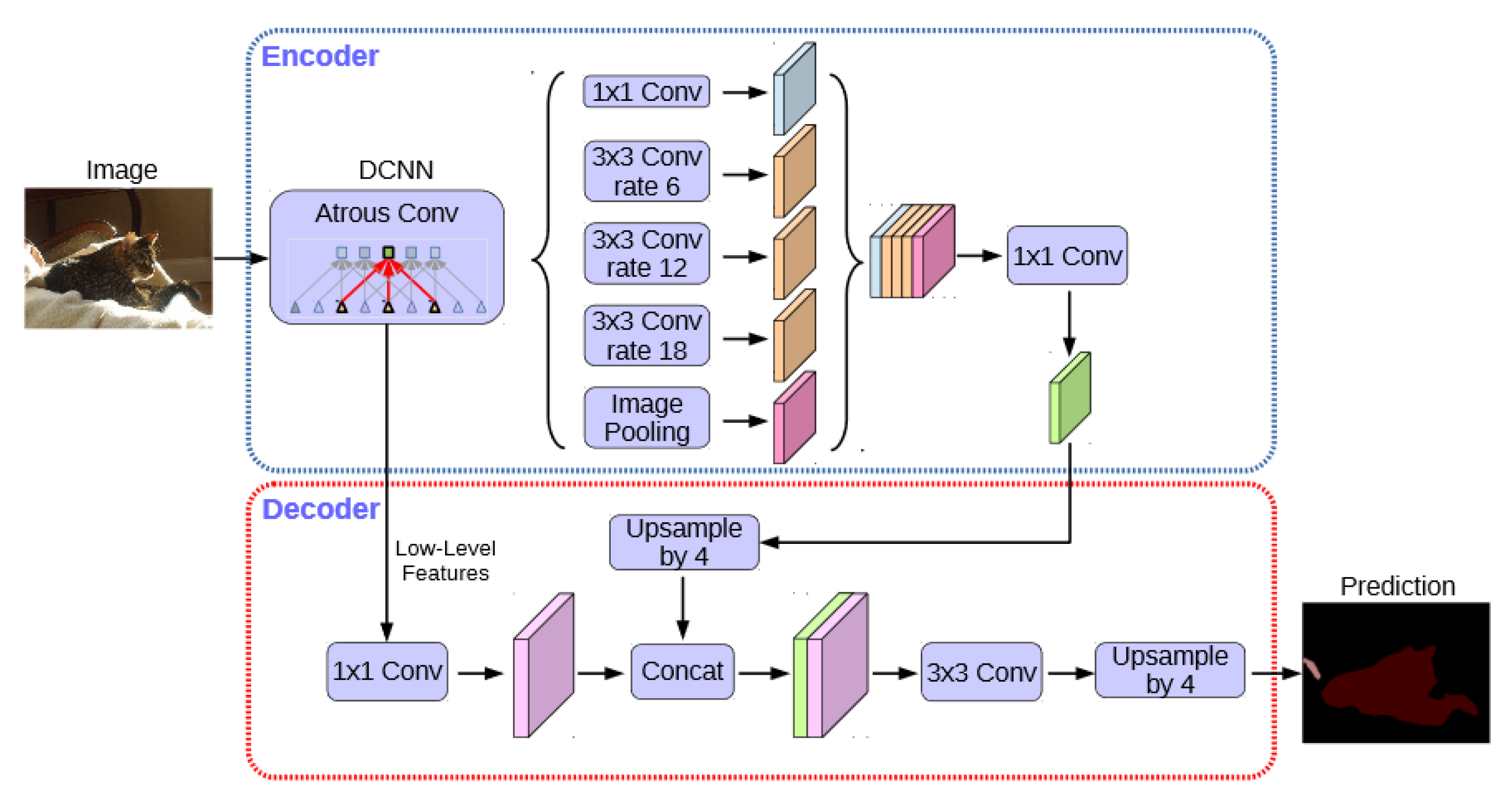
DeepLabV3+ [
25] is a semantic segmentation method that provided very promising results in the PASCAL VOC-2012 data challenge [
26]. For the PASCAL VOC-2012 dataset, DeepLabV3+ has currently the best ranking among several methods, including Pyramid Scene Parsing Network (PSP) [
27], SegNet [
28], and Fully Convolutional Networks (FCN) [
29]. Du et al. [
30] used DeepLabV3+ for crop area (CA) mapping using RGB color images only and the authors compared its performance with three other deep learning methods, UNet, PSP, and SegNet and three traditional machine learning methods. The authors concluded that DeepLabV3+ was the best performing method and stated its effectiveness in defining boundaries of the crop areas. Similarly, DeepLabV3+ was used for the classification of remote sensing images and its performance ranking was reported to be better than other investigated deep learning methods, including UNet, FCN, PSP, and SegNet [
31,
32,
33]. These works also proposed some original ideas to outperform DeepLabV3+ and extend on existing deep learning architectures such as a novel FCN-based approach that aimed at the fusion of deep features [
31], a multi-scale context extraction module [
32], and a novel patch attention module [
33].
In Lobo Torres et al. [
34], a contradictory result was presented in which the authors found DeepLabV3+’s performance worse than FCN. The authors stated that much higher demand for training samples was most likely necessary, which was not met by their dataset, and thus causing DeepLabV3+ to perform below its potential. One other factor contributing to this lower than expected performance could be because they trained a DeepLabV3+ model from scratch without using any pre-trained models as the initial model. There are also some recent works that modify DeepLabV3+’s architecture so that more than three input channels can be used with it. Huang et al. [
35] inserted 3D features in the form of point clouds as a fourth input channel in addition to RGB image data. The authors replaced the Xception backbone of DeepLabV3+ with ResNet101 with some other modifications in order to be able to use more than three input channels with DeepLabV3+.
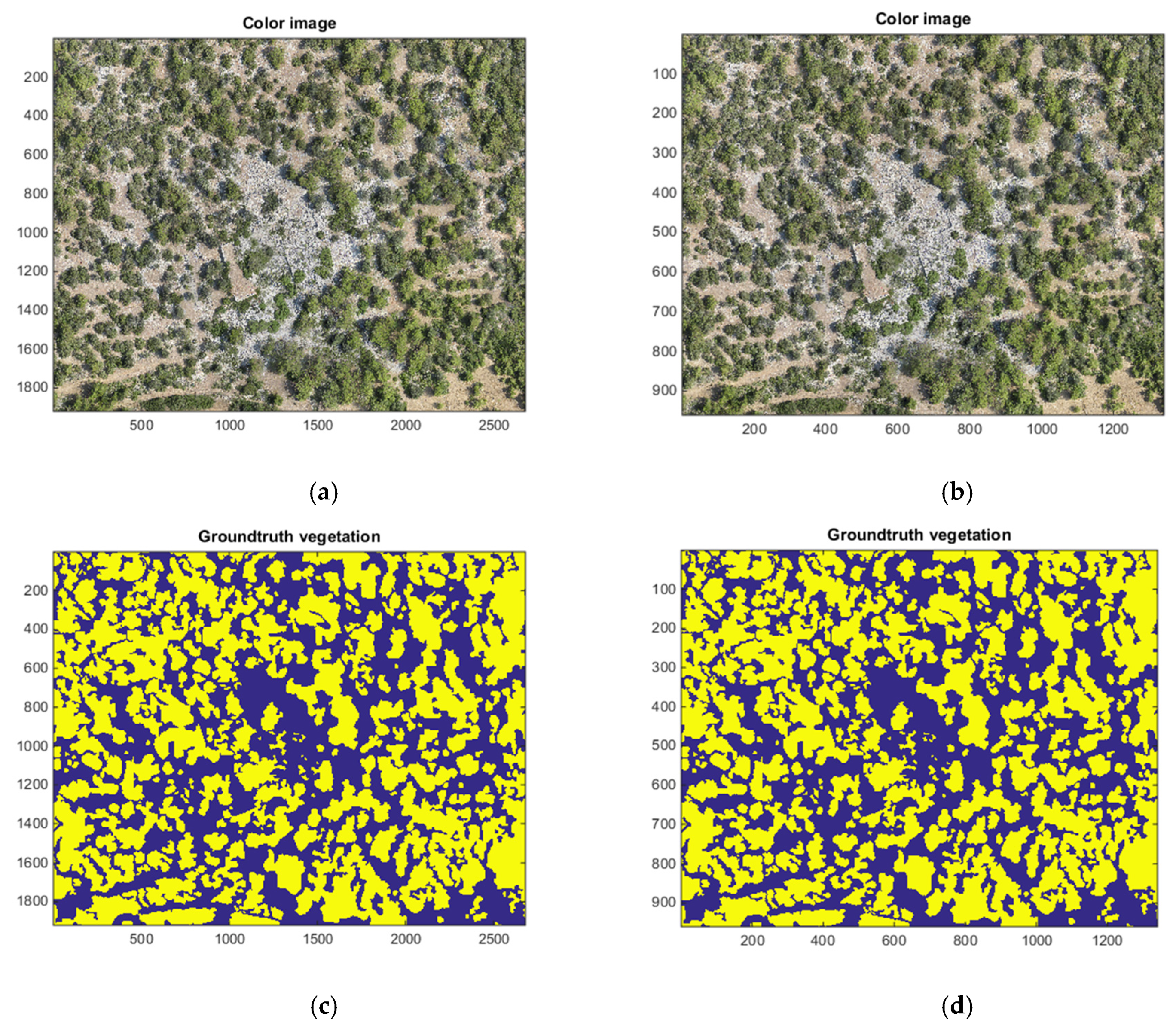
In Ayhan et al. [
5], three separate DeepLabV3+ models were trained using RGB color images originated from three different datasets which are collected at different resolutions and also have a different image capturing hardware. The first model was trained using the Slovenia dataset [
36] with 10 m per pixel resolution. The second model was trained using the DeepGlobe dataset [
37] with 50 cm per pixel resolution. The third model was trained using the airborne high-resolution image dataset with two large size images with the names Vasiliko and Kimisala. The Vasiliko image with 20 cm per pixel resolution was used for training and the two Kimisala images with 10 cm and 20 cm per pixel resolutions were used for testing. It is reported in Ayhan et al. [
5] that, among the three DeepLabV3+ models, the model trained with the Vasiliko dataset provided the best performance and the vegetation detection results with DeepLabV3+ looked very promising.
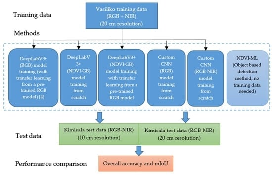
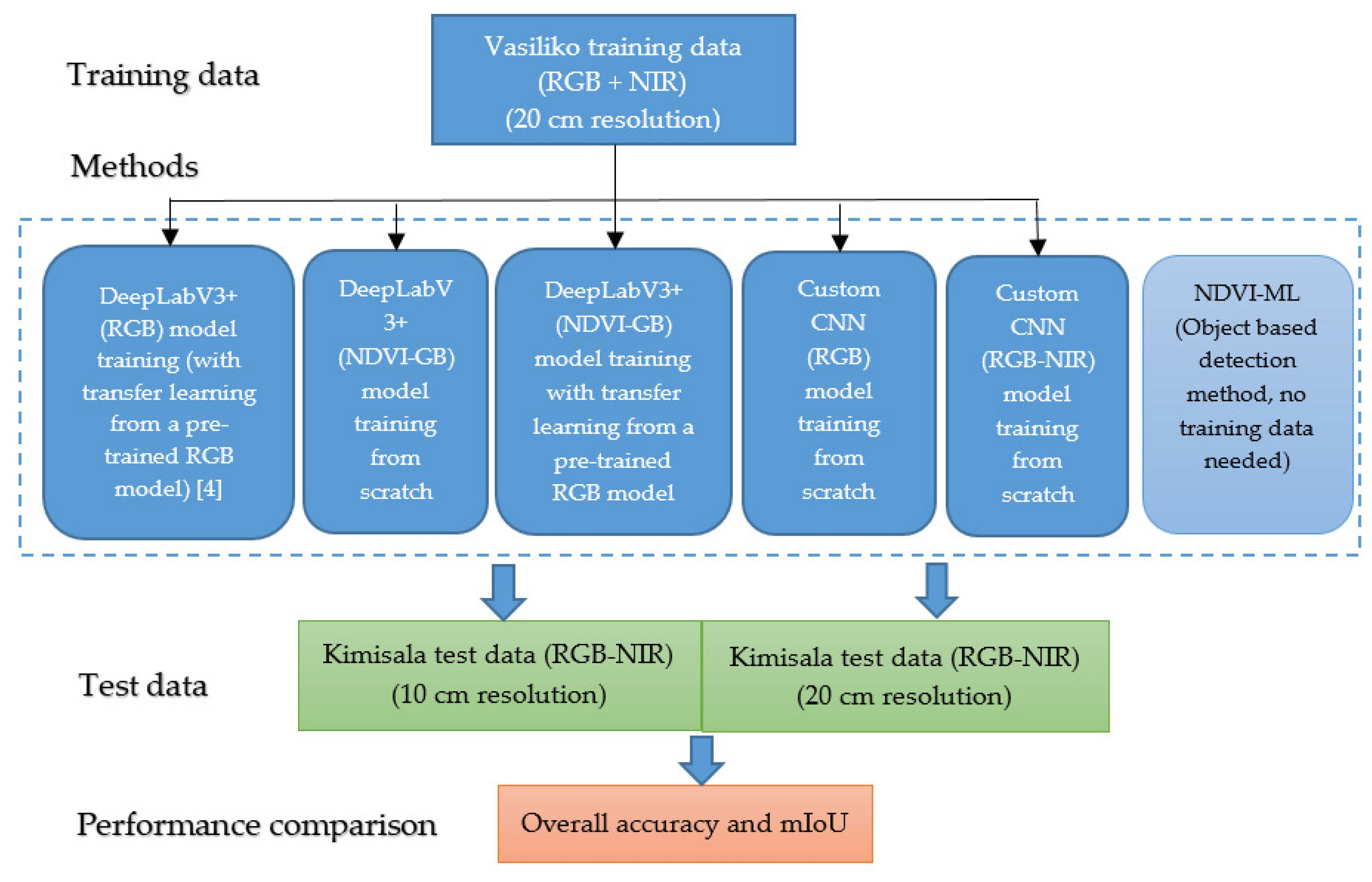
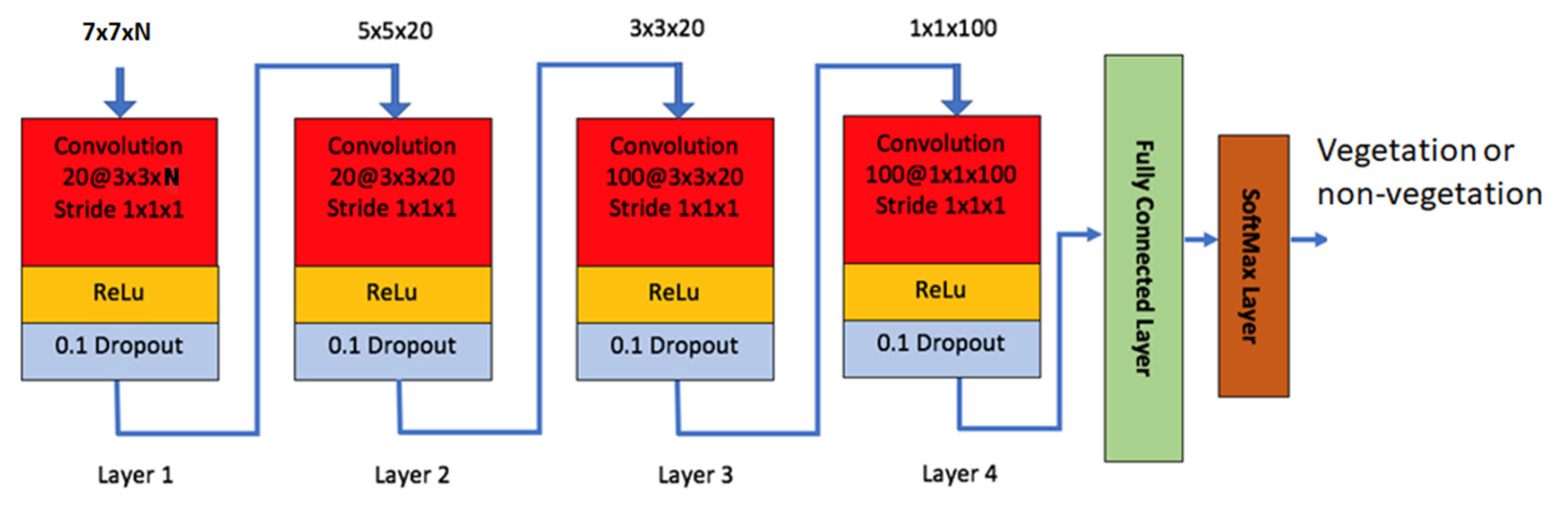
This paper extends the work in Ayhan et al. [
5] by applying DeepLabV3+, a custom CNN method [
38,
39,
40] and a novel object-based method, which utilizes NDVI, computer vision and machine learning techniques on the Vasiliko and Kimisala dataset that was used in Ayhan et al. [
5] for comparison of vegetation detection performance. Different from Ayhan et al. [
5], NIR band information in the Vasiliko and Kimisala dataset is also utilized in this work. The detection performances of DeepLabV3+, the custom CNN method, and the object-based method are compared. In contrast to DeepLabV3+, which uses only color images (RGB), our customized CNN method is capable of using RGB and NIR bands (four bands total). In principle, DeepLabV3+ can handle more than three bands after a number of architecture modifications as was discussed in Huang et al. [
35] and Hassan [
41]. In this work, we used the default DeepLabV3+ architecture with three input channels. However, to utilize all four input channels with DeepLabV3+ to some degree, we replaced the red (R) band with the NDVI band in the training and test datasets, which is estimated by red (R) and NIR image bands, and kept the blue and green image bands to make it three input channels in total, NDVI-GB.
The contributions of this paper are as follows:
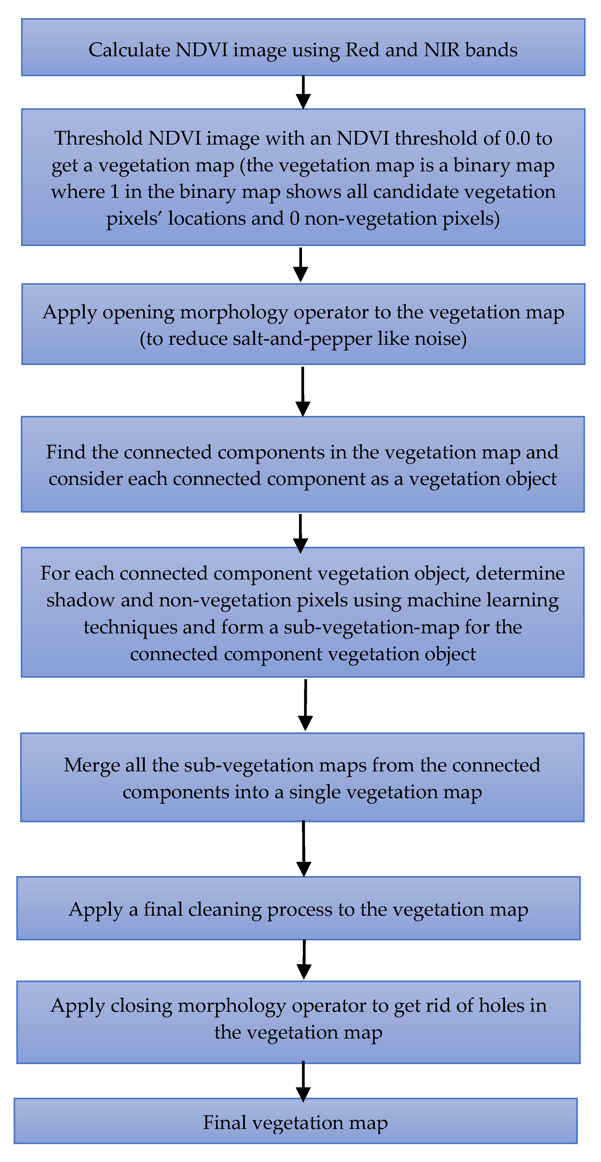
We introduced a novel object-based vegetation detection method, NDVI-ML, which utilized NDVI, computer vision, and machine learning techniques with no need for training. The method is simple and outperformed the two investigated deep learning methods in detection performance.
We demonstrated the potential use of the NDVI band image as a replacement to the red (R) band in the color image for DeepLabV3+ model training to take advantage of the NIR band while fulfilling the three-input channels restriction in DeepLabV3+ and transfer learning from a pre-trained RGB model.
We compared the detection performances of DeepLabV3+ (RGB and NDVI-GB bands), our CNN-based deep learning method (RGB and RGB-NIR bands), and NDVI-ML (RGB-NIR). This demonstrated that DeepLabV3+ detection results using RGB color bands only were better than those obtained by conventional methods using the NDVI index only and were also quite close to NDVI-ML’s results which used NIR band and several sophisticated machine learning and computer vision techniques.
We discussed the underlying reasons why NDVI-ML could be performing better than the deep learning methods and potential strategies to further boost the deep learning methods’ performances.
This paper is organized as follows. In
Section 2, we describe the dataset and the vegetation detection methods used for training and testing.
Section 3 summarizes the results using various methods.
Section 4 contains some discussions about the results. A few concluding remarks are provided in
Section 5.
4. Discussion
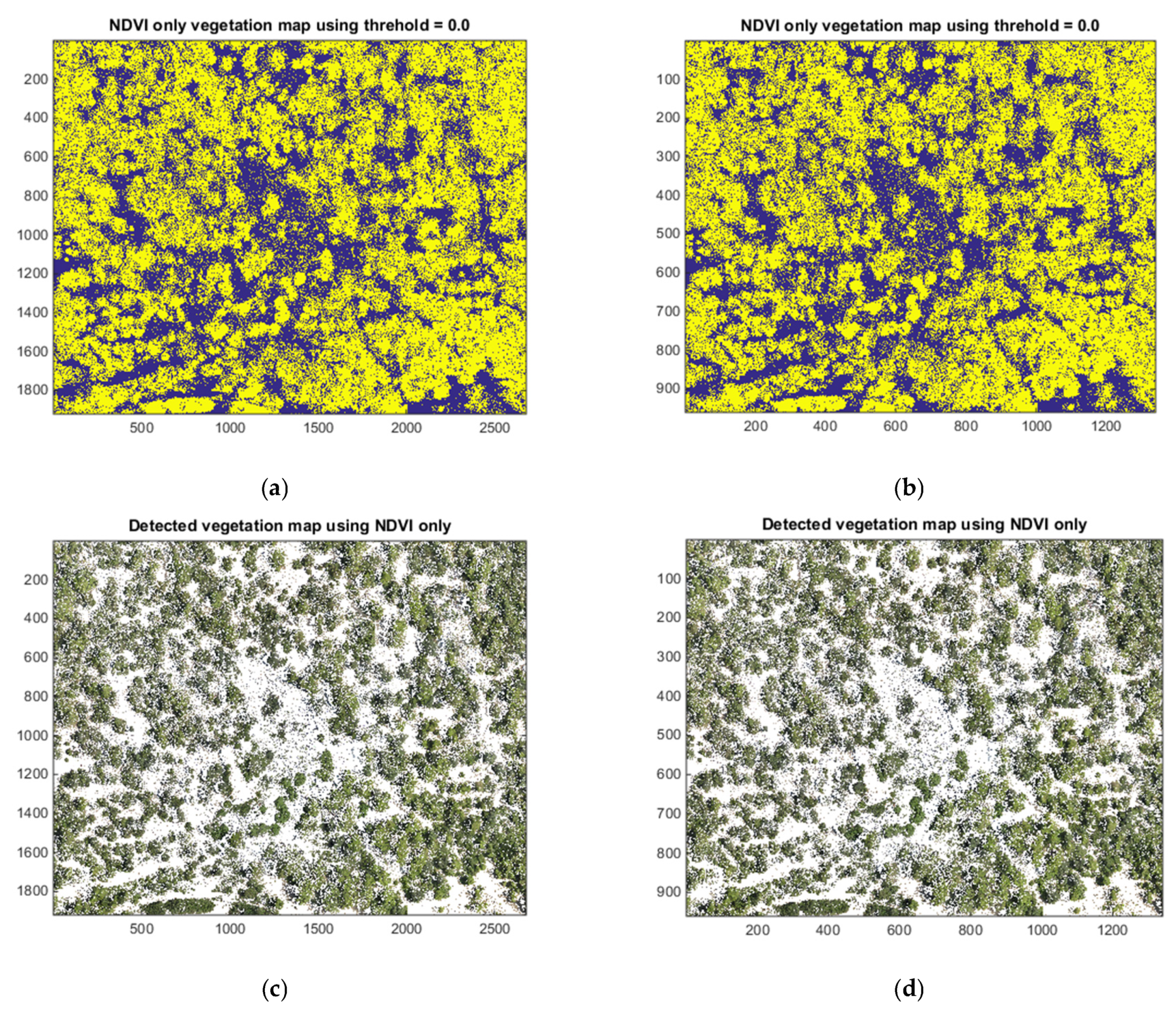
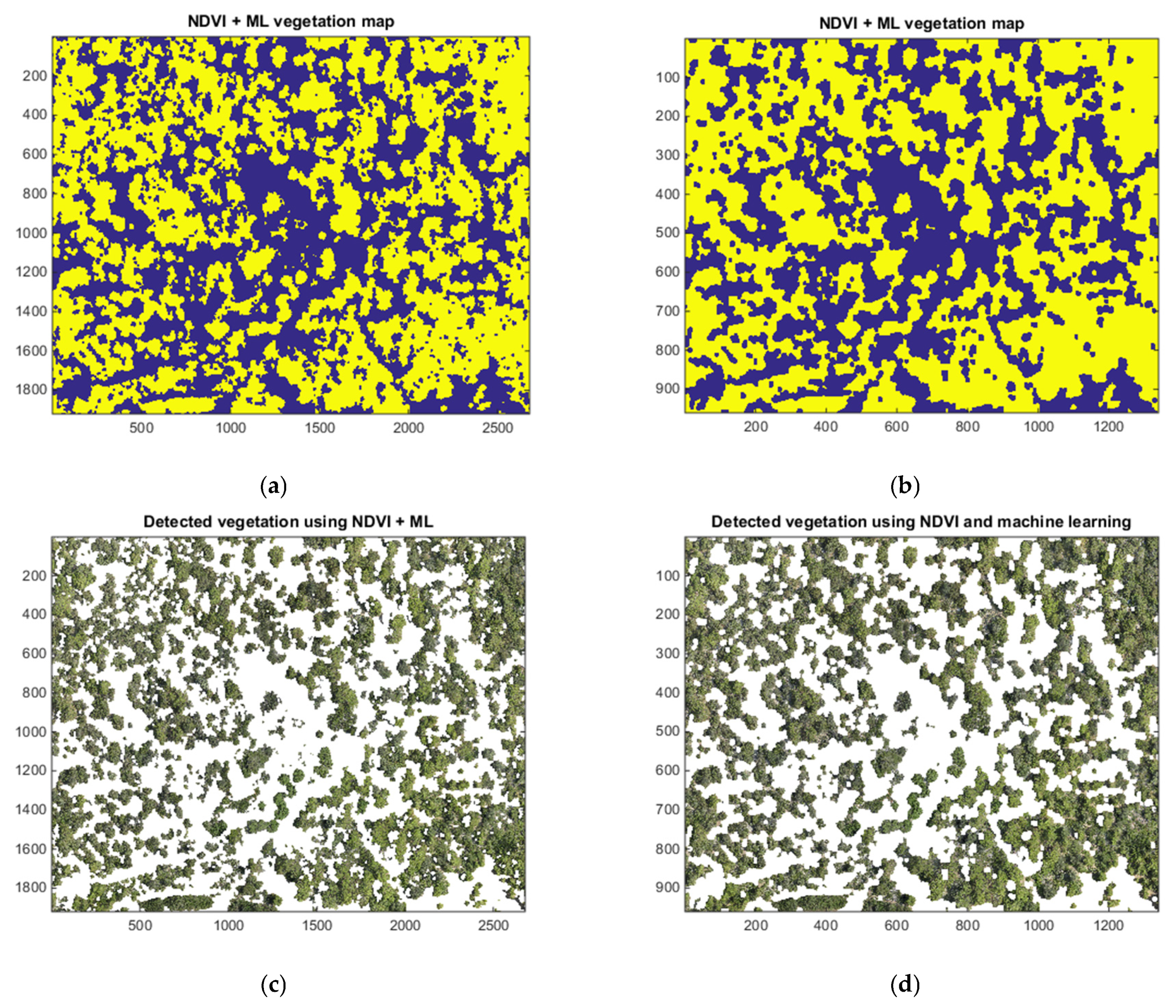
In Kimisala-20 (20 cm resolution) test dataset, DeepLabV3+ (RGB only) had 0.8015 overall accuracy whereas our customized CNN model achieved an accuracy of 0.7620 with RGB bands and reached an accuracy of 0.8298 if the RGB and NIR bands were all used (four bands). The DeepLabV3+ model with NDVI-GB input channels provided an overall accuracy of 0.8089, which was slightly better than DeepLabV3+ model accuracy with RGB channels but lower than our CNN model’s accuracy. Similar trends were also observed in the second Kimisala test dataset that has a 10 cm resolution (Kimisala-10). The detection results for the NDVI-ML method are found to be better than DeepLabV3+ and our customized CNN model for both Kimisala test datasets. For the Kimisala-20 cm test dataset, NDVI-ML provided an accuracy of 0.8578 which was considerably higher than the two deep learning methods.
NDVI-ML method performed considerably better than the investigated deep learning methods for vegetation detection and does not need any training data. However, NDVI-ML consists of several rules and thresholds that need to be selected properly by the user and the parameters and thresholds used in these rules might most likely need to be revisited for another test image other than Kimisala test data. NDVI-ML also focuses on vegetation detection as a binary classification problem (vegetation vs. non-vegetation) since it depends on NDVI for detecting candidate vegetation pixels in its first step whereas in the deep learning-based methods there is the flexibility to classify different vegetation types (such as a tree, shrub, and grass). Among the two deep learning methods, DeepLabV3+, provided extremely good detection performance using only RGB images without the NIR band showing that for low-budget land cover classification applications using drones with low-cost onboard RGB cameras, DeepLabV3+ could certainly be a viable method.
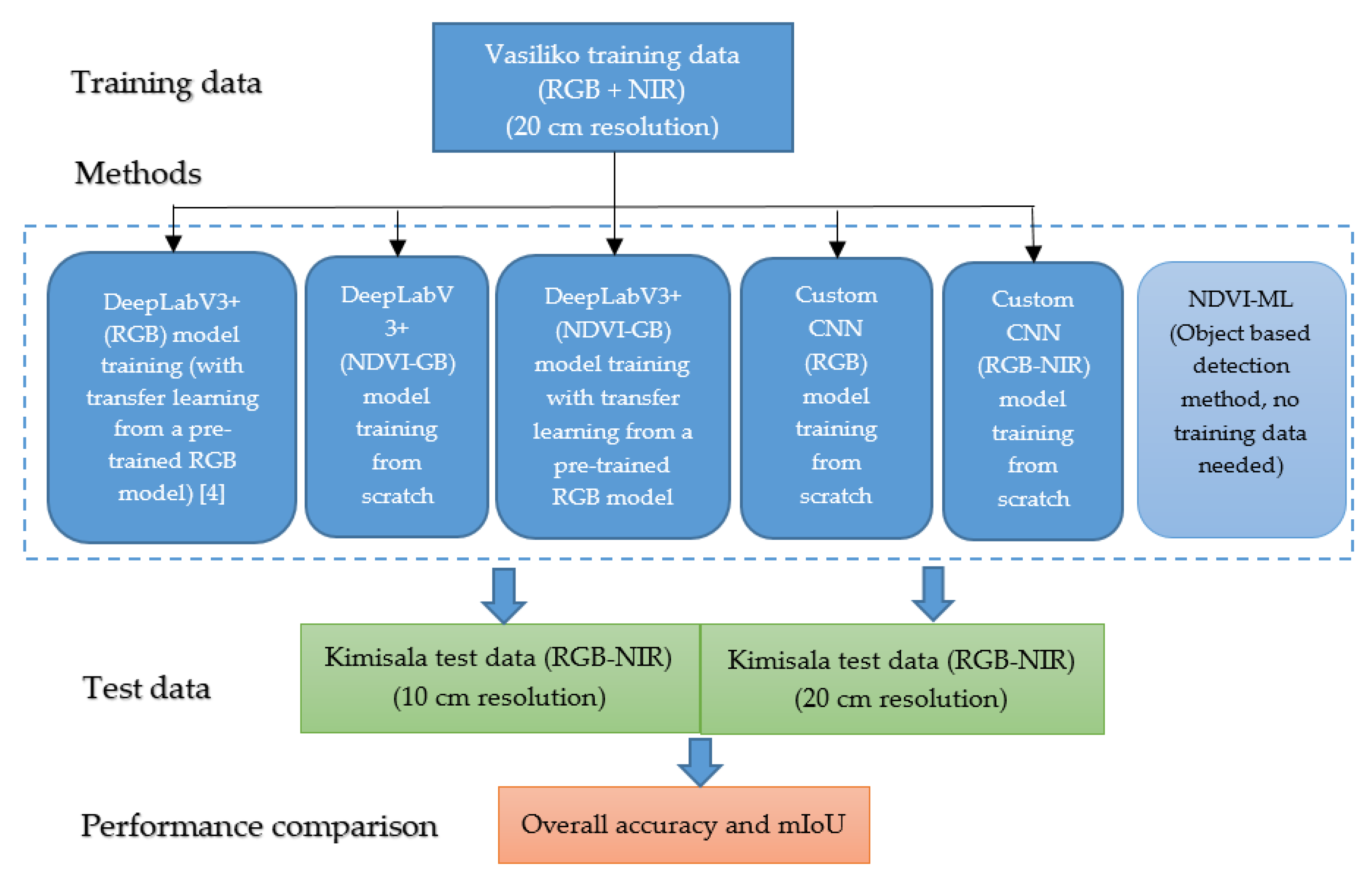
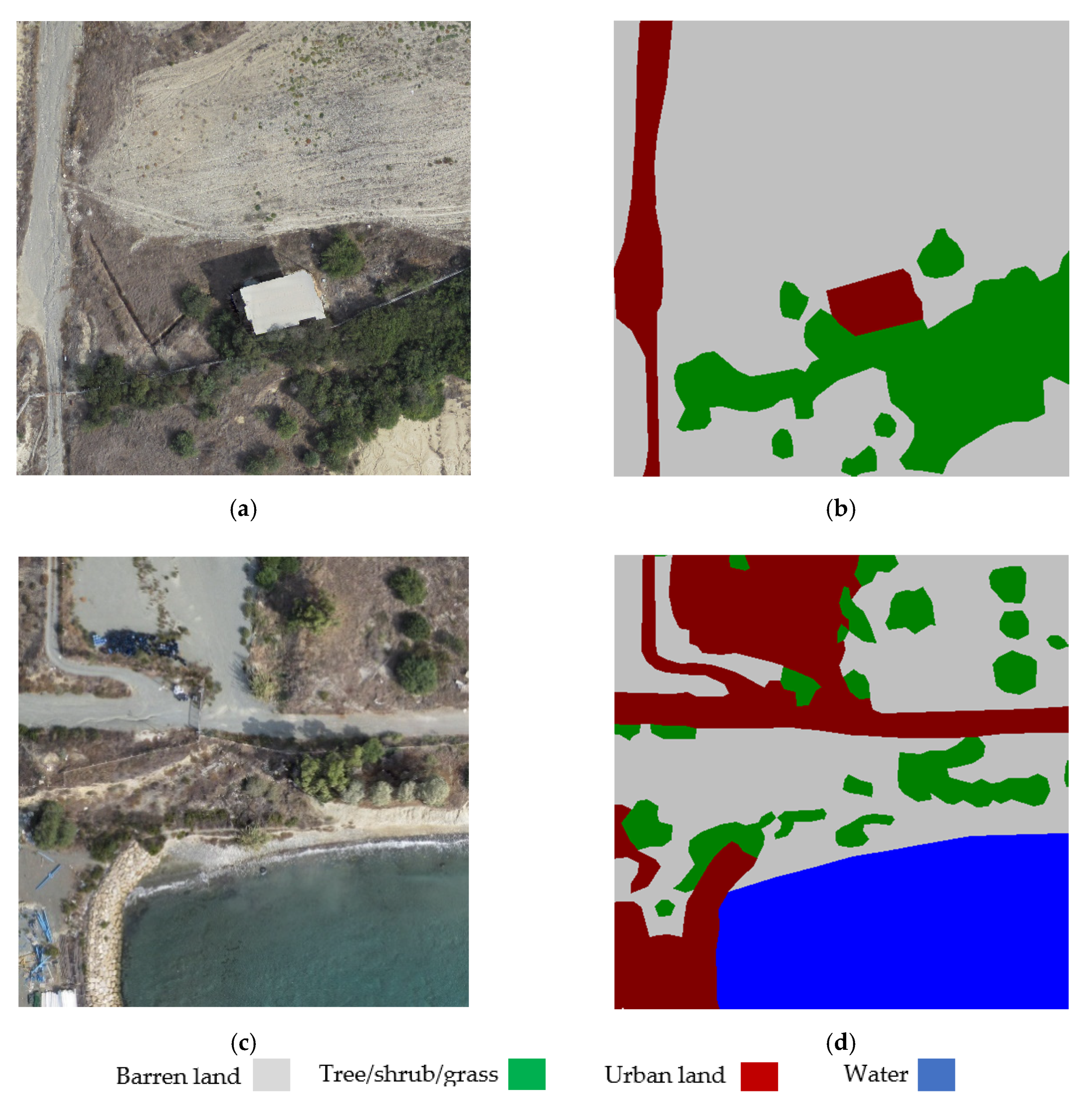
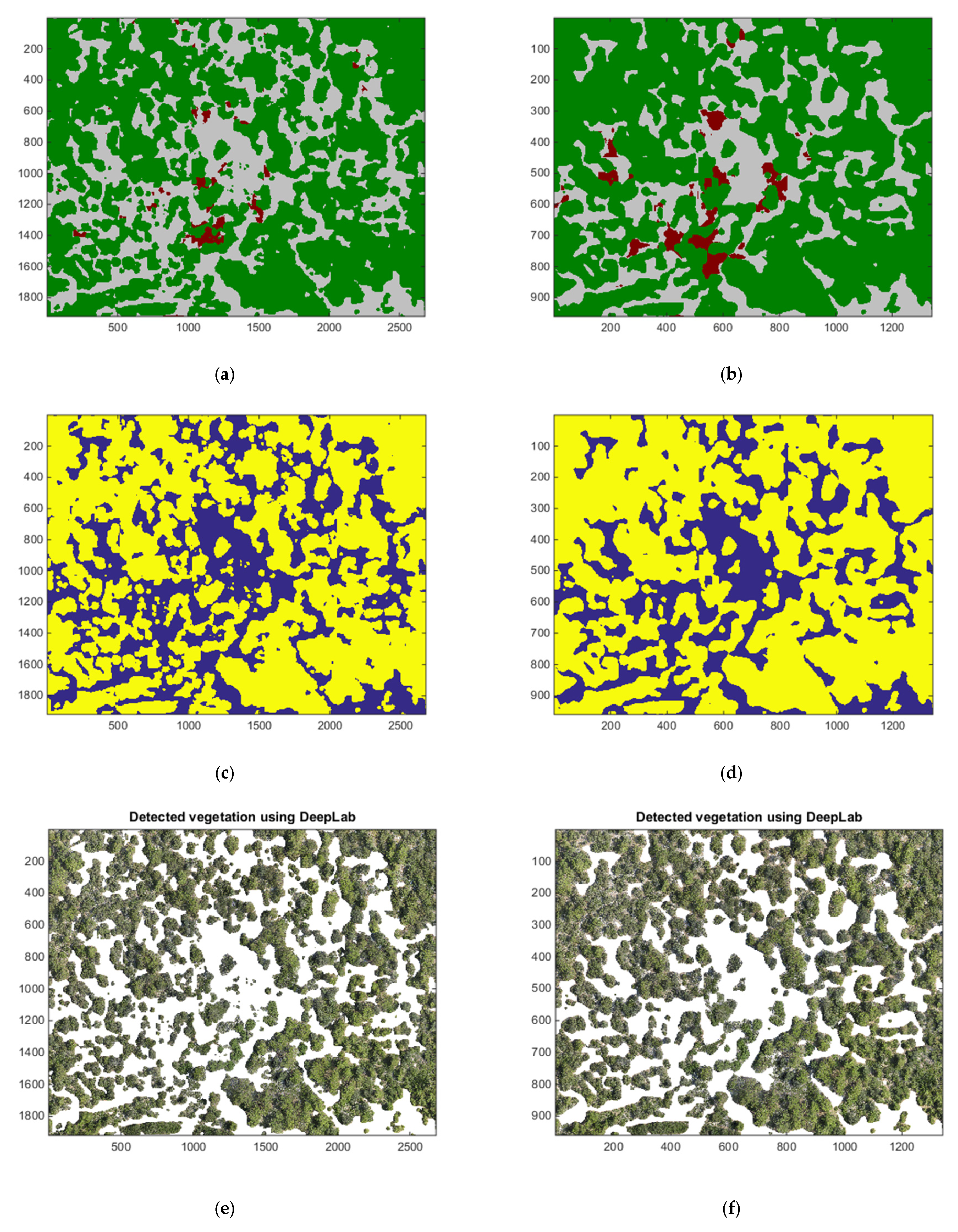
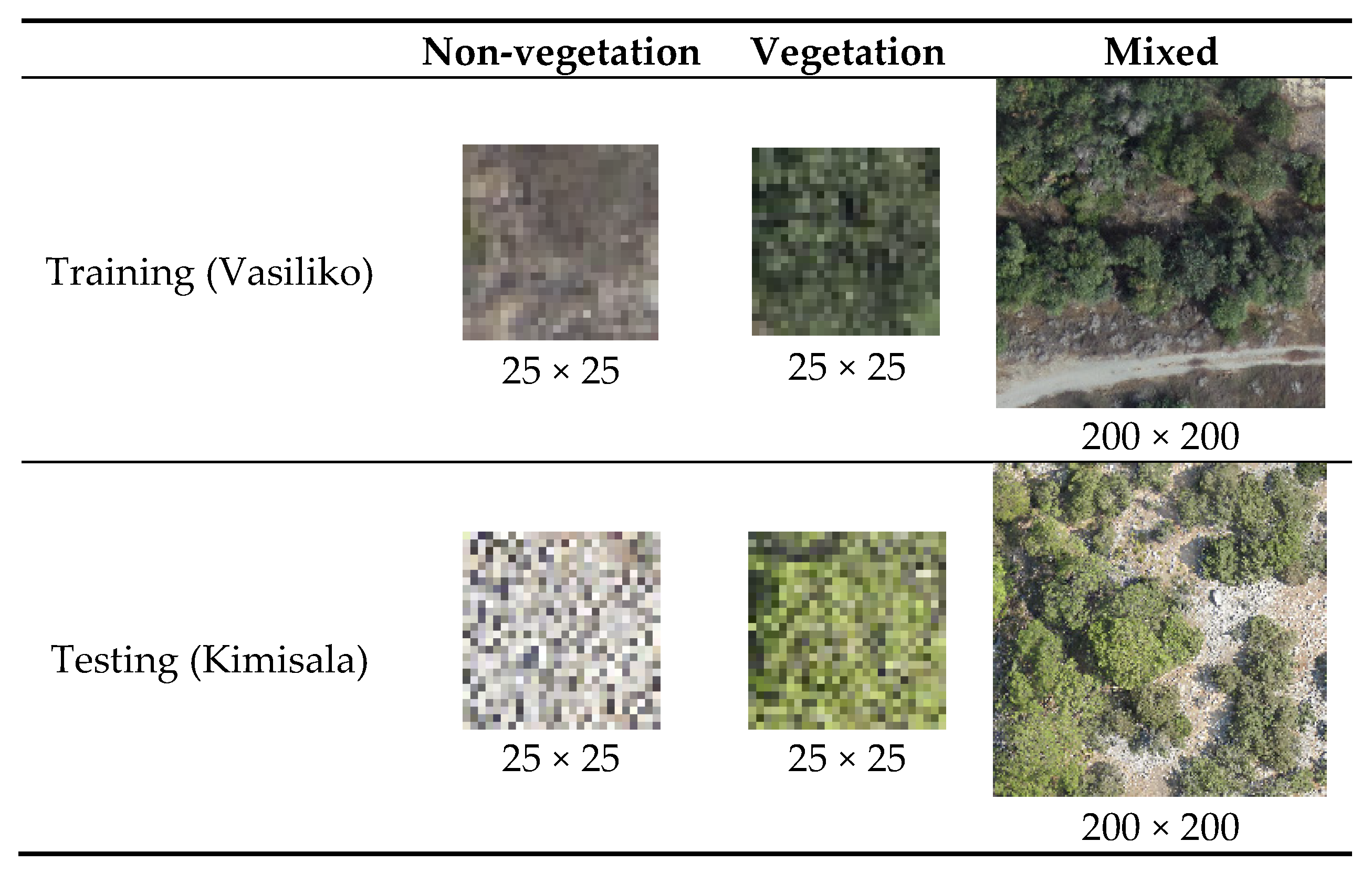
Comparing the deep learning and NDVI-based approaches, we observe that the NDVI-ML method provided significantly better results than the two deep learning methods. This may look surprising because normally people would expect deep learning methods to perform better than conventional techniques. However, a close look at the results and images reveal that these findings are actually reasonable from two perspectives. First, for deep learning methods to work well, a large amount of training data is necessary. Otherwise, the performance will not be good. Second, for deep learning methods to work decently, it is better for the training and testing images to have a close resemblance. However, in our case, the training and testing images are somewhat different even if they were captured by the same camera system as can be seen from
Figure 13, making the vegetation classification challenging for deep learning methods. In our recent study [
5], we observed more serious detection performance drops with DeepLabV3+ when training and testing datasets had different image resolutions, and the camera systems that captured these images were different.
Another limitation of DeepLabV3+ is that it accepts only three input channels and requires architecture modifications when more than three channels are aimed to be used. Even if these modifications are done properly, the training will have to start from scratch since there are no pre-trained DeepLabV3+ models other than RGB input channels. Moreover, one needs to find a significant number of training images that contain all these additional input channels. This may not be practical since the existing RGB pre-trained model utilized thousands, if not millions, of RGB images in the training process. Our customized CNN method, on the other hand, can handle more than three channels; however, the training needs to start from scratch since there are no pre-trained models available for the NIR band.
One other challenge with deep learning methods is when the dataset is imbalanced. With heavily imbalanced datasets, the error from the overrepresented classes contributes much more to the loss value than the error contribution from the underrepresented classes. This makes the deep learning method’s loss function to be biased toward the overrepresented classes resulting in poor classification performance for the underrepresented classes [
50]. One should also pay attention when applying deep learning methods to new applications because one requirement for deep learning is the availability of a vast amount of training data. Moreover, the training data needs to have similar characteristics as the testing data. Otherwise, deep learning methods may not yield good performance. Augmenting the training dataset using different brightness levels, adding vertically and horizontally flipped versions, shifting, rotating, or adding noisy versions of the training images could be potential strategies to mitigate the issues when test data characteristics differ from the training data.

 ,
, 


