Classification of Urban Area Using Multispectral Indices for Urban Planning


1
Department of Geography and Environment, San Francisco State University, 1600 Holloway Ave., San Francisco, CA 94132, USA
2
Estuary and Ocean Science Center, San Francisco State University, 3150 Paradise Dr., Tiburon, CA 94920, USA
*
Author to whom correspondence should be addressed.
Remote Sens. 2020, 12(15), 2503; https://0-doi-org.brum.beds.ac.uk/10.3390/rs12152503
Submission received: 14 July 2020
/
Revised: 31 July 2020
/
Accepted: 2 August 2020
/
Published: 4 August 2020
(This article belongs to the Special Issue Remote Sensing-Based Urban Planning Indicators)
Abstract
:An accelerating trend of global urbanization accompanying population growth makes frequently updated land use and land cover (LULC) maps critical. LULC maps have been widely created through the classification of remotely sensed imagery. Maps of urban areas have been both dichotomous (urban or non-urban) and entailing of discrete urban types. This study incorporated multispectral built-up indices, designed to enhance satellite imagery, for introducing new urban classification schemes. The indices examined are the new built-up index (NBI), the built-up area extraction index (BAEI), and the normalized difference concrete condition index (NDCCI). Landsat Level-2 data covering the city of Miami, FL, USA was leveraged with geographic data from the Florida Geospatial Data Library and Florida Department of Environmental Protection to develop and validate new methods of supervised and unsupervised classification of urban area. NBI was used to extract discrete urban features through object-oriented image analysis. BAEI was found to possess properties for visualizing and tracking urban development as a low-high gradient. NDCCI was composited with NBI and BAEI as the basis for a robust urban intensity classification scheme superior to that of the United States Geological Survey National Land Cover Database 2016. BAEI, implemented as a shadow index, was incorporated in a novel infill geosimulation of high-rise construction. The findings suggest that the proposed classification schemes are advantageous to the process of creating more detailed cartography in response to the increasing global demand.
1. Introduction
Today, the world’s rapidly developing trend of urbanization has made frequently updated surface maps critical [1,2,3,4]. Land use and land cover (LULC) maps are advantageous for purposes of government planning, environmental management, disaster management, and education of the general public on the status of global development. The impacts of urbanization for the environment include triggering potentially harmful feedback such as climate change, reducing water quality, and the replacement of nature by human construction [5,6,7]. The link between urbanization and environmental impacts can be analyzed by mapping their extent and severity in relation to urban expansion [8,9,10]. LULC maps may serve as tools of emergency response to disasters such as fires, earthquakes, and floods where the extent and severity of the disasters can be displayed and analyzed to support response measures. The problem of producing these maps on a large scale can be solved with satellite remote sensing.
Ordinarily, satellite remote sensors feature multiple spectral bands for use in analysis, where each band may be advantageous given the properties of materials identifiable in different parts of the light spectrum [11,12,13,14,15,16,17,18,19,20,21]. Satellite remote sensors take a bird’s-eye view of changes related to urban growth. While high-resolution (1 × 1 m) remote sensing has proven to be very useful for mapping the extent of urbanization as well as for mapping the presence of individual feature footprints, the research presented here focuses primarily on satellites of moderate resolution (10 × 10–30 × 30 m) [12,21,22]. Moderate-resolution data may be sufficient for mapping urban extent and is typically available for free in large time-series volumes compared to high-resolution data which is expensive to acquire, making it unsuitable for institutions with limited budgets.
Typically, satellite image analysts take a dichotomous approach to LULC mapping, classifying image cells as either urban or non-urban [11,12,13,14,15,16,17,18,19]. These maps often depict the encroachment of urban sprawl expanding into the natural landscape. Still, some cities do not grow outwardly because of physical constraints (other cities, terrain, water bodies, etc.) or should not grow outwardly because of planning regulations. The world population is expected to increase from ~8 billion currently to at least 10 billion in three decades, driving the impact of problems associated with urbanization to new levels [4,23]. In response, governments are enacting smart growth policies meant to limit outwardly expanding cityscapes into compact, walkable urban areas with higher populations [3]. Smart growth implies that environmental impacts are lessened by condensing urban infrastructure [3]. Therefore, the drawing of infill development policies is the foremost solution to the problems associated with the outward expansion of cityscapes against the natural landscape [3]. The term infill development refers to the rededication of urban land to new construction. Simply, urban growth takes place within the confines of the cityscape, such as the development of vacant lots, redevelopment of run-down neighborhoods, and conversion of parks to construction.
An inventory of urban land can be obtained through field methods as well as the classification of aerial photographs and satellite imagery and cataloged as data in a geographic information system (GIS). Classifying every land use plot specifically as possible may take a long time, where the necessary geographic view can be achieved more efficiently through a large-scale remote sensing classification. Numerous attempts to classify urban land use by discrete types are on record in scientific journals. Among the methods that may be implemented to create such maps are iterative unsupervised classification, such as k-means and iso cluster, supervised classification requiring class training sets, such as parametric Gaussian maximum likelihood (GML) or non-parametric support vector machine (SVM), and object-oriented image analysis (OBIA) [24,25,26,27,28]. While classifiers by themselves are used to create maps featuring multiple urban types, the process can be refined and simplified using multispectral unsupervised classification formulas called spectral enhancements.
Remote sensing spectral enhancements are formulas used to transform multispectral data retrieved from a sensor into indexed quantities useful for analyzing a target environment, isolating target features, and indexing those features into identifiable classes [8,9,10,11,12,13,14,15,16,17,18,19,20,27,29]. For instance, measurements of solar radiation reflecting from Earth’s surface to a satellite sensor can be manipulated to yield a description of plant biology, the presence of bare soil, or a state of urbanization [12]. For example, Zha et al. (2003) [18] introduced a method for extracting urban features from satellite data using a spectral enhancement. The normalized difference built-up index was used to extract urban features of Nanjing, China from Landsat 5 Thematic Mapper (TM) 30 × 30 m resolution data. It enhances the spectral response differences that exist between shortwave infrared (SWIR) and near-infrared (NIR) bands to separate urban from non-urban areas in an image. The authors reported an accuracy of 92.6% based on an assessment of 68 randomly distributed points in their study area and assert that spectral enhancements increase urban feature classification accuracy compared to the GML classifier.
Ettehadi et al. (2019) [27] mapped the land cover of Istanbul by classifying enhanced images, derived from Sentinel-2A 10 × 10–20 × 20 m data, using SVM. The normalized difference tillage index was used to highlight urban features as part of a three-band composite image, including the red-edge-based normalized difference vegetation index, and the modified normalized difference water index. They delineate asphalt, industrial land use, and other built-up as part of their classification scheme. The reported producer and user accuracies are 85.71% and 100% for asphalt areas, 98.28% and 81.43% for industrial areas, and 93.28% and 92.25% for other built-up. It is of critical notice that differences in environmental factors like lighting, the complexity of land cover, etc. that occur between regions will impact the performance of enhancements [12]. While there is record of successful methodology for classifying discrete urban land use types with moderate resolution data, in addition to methodology for extracting feature footprints from high-resolution satellite imagery, research still needs to be conducted for extracting the footprints of urban land use geometries (recreational, residential, business, etc.) from moderate resolution data [21,22,27]. Additionally, though the state of environmental variables are frequently measured with low-high gradients, such as the use of the well-known normalized difference vegetation index (NDVI) to measure plant vigor, there is no volume of knowledge available about measuring the state of urban development by gradient [8,9,10,29].
The United States Geological Survey (USGS) publishes the National Land Cover Database (NLCD), derived from Landsat data and delineating all land in the conterminous United States into 21 classes, every five years. NLCD features four classes of urban intensity derived entirely from the NLCD Percent Developed Imperviousness product, also released on the same five-year basis. The classes are open space, low intensity, medium intensity, and high intensity. Open space is typified by mostly vegetation (<20% impervious), low intensity by single-family homes (20–49% impervious), medium intensity by single-family homes (50–79%), and high intensity by frequently traversed areas (80–100% impervious) [30]. These urban intensities are based on groupings of developed surface imperviousness derived from satellite data, which physically limits the interpretation of feature structure. There is room in scientific writing for a methodology, emphasizing automation, for correcting the linear errors associated with deriving classes from only a satellite assessment of surface imperviousness.
In addition to static classification maps, urban growth models, called geosimulations, are used to generate land cover maps of predictable conditions by assigning transition probabilities and potentials to maps derived from remote sensing [1,2,3]. Rahimi (2016) [3] utilized a combination of GIS, remote sensing, and a multilayer perceptron (MLP) artificial neural network (ANN) in an attempt to map potential infill development for the city of Tabriz, Iran. Urban land cover was classified, cell-by-cell, as either urban or subject to infill development. LULC classifications were derived from Landsat 5 data for 1989 and Satellite Pour l’Observation de la Terre (SPOT) 10 × 10 m data for 2005. The classifications were cross-referenced with geographic predictor variables such as distance from roads and population density using an MLP ANN geosimulation, thus predicting urban land cover for 2021. Sun et al. (2007) [1] modeled the growth of Calgary, Canada, using a cellular automata/Markov chain combination model. They predicted change, using classified Landsat 5 data from 1985 and 1992, regarding the presence of residential and commercial, industrial, transportation, and park development compared to vacant areas and water bodies. Suitability maps of Calgary’s “Future Conceptual Urban Structure” were created for each class, merged, and used as a predictor. The researchers were able to achieve favorable results according to a cellular accuracy assessment using data of known conditions of the predicted year, 1999. Where geosimulations of varying accuracy are on record, a knowledge gap exists concerning the difficulty of predicting discrete changes, such as the construction of skyscrapers, on a cell-by-cell basis [1,2,3]. There should be research of methodology for geosimulating a prediction encompassing the formation of such changes.
The purpose of this paper is to advance our current understanding of the processes of leveraging remote sensing to identify discrete urban land use types for incorporation into modeling schemes such as static mapping and geosimulations. The study evaluated the possibility of implementing spectral enhancements designed to enhance construction features from the natural landscape for the creation of new classification schemes that delineate urban land use types. It seeks to establish means of separating urban features captured in enhancements by distinguishing identifiable attributes such as albedo, the scale of development, and surface configuration. Today’s GIS software packages include intuitive tools for performing the necessary geospatial analyses such as pixel-based image classification and OBIA, time-series change detection, and conditional geoprocessing. The aim is to propose new schemes, based on enhancements, for classifying urban land using:
- Classification by object: Urban land use types may be identifiable by differences in albedo attributed to the presence of varying construction materials, vegetation, and bare ground.
- Classification by gradient: The amount of radiation absorbed by urban surfaces may fluctuate due to deconstruction (i.e., by natural disasters) or the accumulation of construction material (i.e., by infill development).
- Classification by intensity: Urban feature structure may be mapped by compositing the properties of albedo, absorbed radiation, and percent of developed imperviousness.
- Classification by focalized transition potential; development trends attributed to discrete occurences identifiable in imagery may be generalized to accurately predict the extent of those occurences.
The enhancements analyzed are the new built-up index (NBI) by Jieli et al. (2010) [14], the built-up area extraction index (BAEI) by Bouzekri et al. (2015) [12], and the normalized difference concrete condition index (NDCCI) by Samsudin et al. (2016) [20]. NBI yields a low-high assessment of surface albedo, which may be useful for discriminating groups of urban features according to their relative brightness. BAEI works as a view of the surface net radiation balance (NRB), wherefore it may be possible to measure the amount of construction material present on the surface. The NDCCI band configuration differs slightly from NDVI, designed to focus on construction instead of vegetation, which may make it more useful for urban mapping. Urban intensities published by the USGS in NLCD 2016 are analyzed for classification errors, and a corrected classification was modeled with the NLCD 2016 Percent Developed Imperviousness product in tandem with SVM supervised and iso cluster unsupervised classifications of an NBI/BAEI/NDCCI composite. A novel geosimulation of high-rise development was performed with land use classifications derived from the BAEI as a shadow index, based on focalized index values integrated with manual classifications and using polynomial transition trends as predictors.
2. Methods
ESRI’s ArcGIS [31] was the software used in most of the study; for geoprocessing, geospatial analysis, and cartography. ERDAS Imagine [32] was used for image histogram analysis to establish BAEI feature extraction thresholds. Clark Lab’s TerrSet [33] was used for geosimulating future land use with the land change modeler (LCM) module for MLP ANN Markov chain analysis. The research was conducted on a place with satellite coverage, where urban growth modeling is highly relevant to environmental sustainability and can be validated using a sufficient volume of ground truth data.
2.1. Study Area
Miami, FL, USA is located on the southeastern tip of Florida at 25°46′29.8128″N/80°11′9.5604″W, spans ~143 sq km, and serves as the Miami-Dade County seat (see Figure 1). The land use types comprising the city are primarily residential, commercial, and industrial. Miami poses a unique challenge to the science of urban remote sensing. It does not grow outwardly because other cities and development border its western periphery, and its eastern boundary is the coastline. It is a rapidly developing metropolis with a recorded population increase of ~350,000 in 1980 to ~486,000 in 2018 [34]. Miami-Dade County has enacted development concurrency policies meant to force a compact urban design by slowing sprawl and promoting infill development [35]. For instance, some areas of Miami became hotspots for construction of multifamily housing between 1995–2004, after the inception of Transportation Concurrency Exception Areas that allow for infill development despite traffic and accessibility limits [35]. A coastal setting containing sensitive marine environments makes this city a highly relevant target for an inquisition into environmental conservancy by actively managing urban growth. If remote sensing is implemented as a means of monitoring Miami’s growth, it should be modeled to account for upward growth. A collection of cloud-free Landsat data is available from the USGS in addition to volumes of GIS data provided by the state of Florida and Miami-Dade County.
2.2. Data Sources
Vector GIS data of Miami were retrieved from Miami-Dade County Open GIS. That dataset includes shapes of the Miami municipal boundary, county water features, and the shoreline. Florida neighborhood shapes were retrieved from Zillow Real Estate Listings. Finally, shapes of Florida LULC designations were retrieved from the Florida Geographic Data Library (FGDL) and the Florida Department of Environmental Protection (FDEP) Geospatial Open Data. The LULC designation files were converted to 30 × 30 m raster format to facilitate cell-by-cell analyses. The GIS data are used to clip and analyze select portions of satellite data acquired from the National Aeronautics and Space Administration (NASA) Landsat satellite series. NLCD 2016 data were published by the USGS.
According to the USGS [36], the 30 × 30 m Landsat Surface Reflectance Level-2 science data that is available free to the public from their EarthExplorer website is designed to support the analyses of land change science. Level-2 data is preprocessed with both georeferencing and atmospheric corrections to normalize every image in the dataset for comparison [36]. Level-2 Landsat 5 data receive atmospheric corrections in the form of 6S (Second Simulation of a Satellite Signal in the Solar Spectrum) meant to minimize the influence of water vapor, ozone, geopotential height, aerosol, and elevation on spectral returns [36]. Similarly, Landsat 8 Operational Land Imager (OLI) data is corrected with an internal satellite algorithm [36]. All Level-2 images used for this study are georeferenced to the Universal Transverse Mercator (UTM) Zone 17N projected coordinate system [36]. Subsequently, all other data was initially projected to this system to facilitate analysis, except for the NLCD products.
The imagery used in this study includes Landsat 5 data for the dates of 2 November 1985, 6 November 1998, 24 October 1999, 20 November 2003, 17 November 2008, 19 October 2009, 2 November 2011, and Landsat 8 data for the dates of 17 October 2014 and 22 October 2016. The temporal sequencing of the data was intended to minimize the spectral influence of differences that will occur because of seasonal conditions. Due to sensor saturation, the data may contain minor errors that pitch some cell values outside of the 0-1 range of proper reflectance values. These cells are screened out of each band during geoprocessing to preserve analytical accuracy. Table 1 lists all of the GIS and remote sensing data used, including the year or date covered by the data, sources, file formats, and the amount of land cloud cover in imagery as estimated by the USGS.
2.3. Evaluation of Published Built-Up Indices
Landsat data were used to evaluate eleven enhancements by visual assessment of the study area, including the adjustment of symbology and display settings. The enhancements were selected through rigorous review of scientific literature relevant to urban feature extraction, where each index was found to be well-known or recently published. Nine were designed to extract urban features from moderate resolution data, one designed to extract urban features from SPOT data, and one designed to assess the quality of building materials with high-resolution data. The enhancements were initially derived from the 2016 Landsat 8 image, and a time-series incorporating all of the images was evaluated for BAEI. A list of these enhancements is given in Table 2. The three enhancements selected for further analysis, based on the identification of unique spectral properties previously undocumented in published research, were NBI, BAEI, and NDCCI (see Figure 2).
2.4. Evaluation of the New Built-Up Index for Object-Oriented Urban Feature Extraction
Upon visual assessment, NBI showed pronounced differences between areas of Miami that are known to possess business infrastructure compared to those that are known to possess no infrastructure or residential land use. Therefore, it was selected for further evaluation regarding its usefulness for serving as the basis of an object-oriented urban land use classification scheme. Jieli et al. (2010) [14] developed this index with Landsat 5 data to automate the process of mapping residential areas of Changzhou City, China. The researchers report an overall accuracy of 90% based on a survey of 50 random points in their study area.
An index raster derived from the 2016 Landsat 8 data was clipped to the shape of Miami without feature extraction thresholding. While visual assessment yielded the conclusion that it is easy to spot differences between one type of urban feature and another in an enhanced image, the point requires further elaboration. Noticeable differences exist among land cover types captured in satellite data between the red, NIR, and SWIR1 bands, and the NBI band arrangement yields an unsupervised classification where the brightest features (typically urban or barren land) have the highest values [14]. Thus, index values for areas that are only urban will show enhanced brightness for features with high albedos, such as white concrete or the bare ground of construction sites. Subsequently, zonal statistics describing the central tendency of index values were calculated for each land use type featured in the FGDL data. It must be noted that FGDL data does not feature polygon geometries for streets and is advantageous because it contains additional details regarding the presence of industrial development compared to the data from FDEP. ArcGIS includes the Mean Segment Shift interactive OBIA tool for grouping parts of an image with similar properties into segments.
Phiri & Morgenroth (2017) [37] define OBIA as the automatic digitization of homogenous image features. It works by grouping pixels into vectored segments and then assigning a class to like segments [37]. Segments are defined by spectral, spatial, and geometric properties [37]. Spectral detail refers to color characteristics, such as the difference between one type of commercial construction and another. Spatial detail refers to identifiable differences in spatial characteristics, such as street lines compared to residential blocks. Geometric detail refers to the minimum size of an image segment, which can aggregate details on, for example, a pixel, block, neighborhood, or city level. The method is useful for avoiding a scattered, “salt and pepper” look typically associated with pixel-based classification methods.
The 2016 NBI was segmented into object primitives useful for identifying enhanced color intensity, object formation, and surface texture. An object encompassing industrial land use in the Little Haiti neighborhood of Miami was extracted by vectorizing a segment. The object was cross-referenced with the FGDL data to validate the usefulness of non-automatic, interactive segment selection as a classification method. While discrete urban types can be classified through OBIA feature extraction with this index, there is still an additional need for analysis of the scale of development within classes.
2.5. Evaluation of the Built-Up Area Extraction Index for Change Detection of Gradient Development
BAEI provides an enhanced view of the accumulation of construction material as a low-high gradient. The index was selected for further evaluation regarding its usefulness for time-series change detection of a quantifiable increase in urban development (different grades of building presence) because of its range of non-linear values, which may prove useful for tracking shifts in urban morphology. In addition to a pronounced gradient, the index feature extraction threshold separates high-rise shadows from the rest of the urban area.
BAEI is a high-precision, non-linear (the positive range of values extends beyond 0 to 1) feature extraction index developed with Landsat 8 data by Bouzekri et al. (2015) [12] to automate the process of extracting built-up areas of Djelfa, Algeria. They report an accuracy of 92.66% based on a survey of 50 random points in their study area. Compared to the other built-up indices evaluated, it provides an expanded range of values that may be useful for classifying urban states with low-high values. An observable increase in the central tendency of index values for an urban area, over a time-series, requires additional explanation.
Chrysoulakis (2003) [38] utilizes NASA’s Advanced Spaceborne Thermal Emission and Reflection Radiometer 15 × 15–30 × 30 m satellite data, in combination with in situ data, to develop an estimation of the all-wave surface NRB for Athens, Greece. NRB is defined in the formula:
where αshort is surface total shortwave albedo, E is direct and diffuse shortwave irradiance on the surface, F ↓ is atmospheric downward longwave flux, and F ↑ is total surface radiant exitance. Highly developed areas, such as business and stadiums, should possess a lower NRB because the higher albedos of bright construction materials typify them and therefore absorb less radiation than areas with lower albedos, such as areas of medium development or vegetated spaces [38]. Also, urbanization influences the distribution of heat fluxes related to NRB with a combination of drivers, including replacement of vegetation with construction, reduced surface moisture, and the complexity of urban morphometry [38]. BAEI is an expression of NRB, with low values for highly developed areas, mid-ranged values for medium development, and high values for areas that are vegetated or comprised of dark asphalt. Where index values increase over time, the increase is linked to the influence of human beings on NRB, since NRB will rise for reasons linked to human development.
NRB = (1 − αshort)E + F ↓ − F ↑
To validate this index as automatic, unsupervised classification of different grades of building presence, an evaluation was made of the usefulness of the index to chronicle stages of urban growth for Miami using the mean as a measure of central tendency, including the influence of vegetation. Enhancements were derived for six satellite images in a time-series spanning 1985–2016. If thresholds are not applied, BAEI rasters for Miami are highlighted by the formation of shadows cast by high-rise infrastructure in downtown neighborhoods. The visualizations need to be refined by omitting the formation of shadows to display an enhanced gradient visualization of an urban environment.
Histogram analysis is a method for identifying a statistical break in the range of index values that will extract the target features from the rest of the data [39]. Thresholds were determined through a trial-and-error process of raster histogram analysis performed in Imagine to establish the best visual fit for separating shadows. BAEI rasters were geoprocessed with conditional thresholds for Landsat 5 and Landsat 8. Note that conditional thresholds of 2.5 and 2.4 were assigned to Landsat 5 and Landsat 8, respectively, to enhance visualizations. A different threshold for Landsat 8 is necessary because it possesses different spectral bandwidths and cannot be directly cross-referenced with Landsat 5. Cross-referencing can be performed with post-classification image comparison and post-classification change detection.
A visual and statistical comparison was made of the time-series for the entire city. Due to the apparent influence of urban canopy in the southern portion of the city on index values in the first time-series, a shape truncated of the three southernmost neighborhoods was created. Rasters clipped to the truncated area were necessary to evaluate how well this index tracks the accumulation of constructed features over time as opposed to the accumulation of urban arbor. Further scrutiny was given to the truncated area concerning the influence of vegetation.
NDVI has widely proven useful in classifying the presence and vigor of plants visible in remote sensing data [8,9,10,29]. Index values are linear, −1 + 1, with values in the direction of 1 indicating the presence of healthy vegetation.
NDVI = (NIR − RED)/(NIR + RED)
NDVI was derived for a time-series of the truncated area for statistical and visual comparison. Note that Miami-Dade County does not possess significant arbor compared to other urban areas in the United States, having 20% tree cover in 2016 [40]. Zonal statistics for BAEI and NDVI were calculated using the truncated area for a time-series of nine images spanning 1985–2016.
BAEI, utilized as a shadow index by not thresholding the raster, displays values for Miami with a pronounced division between the shadows cast by high-rises and other urban area. Shadows are focalized and further analyzed by establishing a threshold to separate cells that highlight shadows. Subsequently, a time-series of urban land use classification maps incorporating the extracted shadow highlights was created to depict a formation trend. A geosimulation incorporating a 2003 and 2008 image time-series in combination with directional land use polynomial transition trends as predictors was performed to predict the construction of high-rise infrastructure for 2016 in the Brickell neighborhood (see Section 2.7). Consideration was given regarding how NBI and BAEI may be composited to take advantage of the useful properties of both enhancements.
2.6. Evaluating the Normalized Difference Concrete Condition Index for Incorporation in Urban Development Intensity Classifications
It is possible to composite enhancements as an image stack, whereby the desirable properties of each enhancement can be translated to a single output. NDCCI derived from the 2016 Landsat 8 data visualized Miami’s urban fabric as a network of streets containing pronounced areas of low development, collections of homes, and varying stages of development in areas of business and dense transport. Consideration was given to this index as the basis for an enhancement composite with NBI and BAEI based on a comparison of zonal statistics with NDVI referencing urban land use types. The composite was then classified to identify pronounced spectral groupings based on the feature extraction achieved by combining enhancements. That is to say, differing states of urban intensity are delineated according to their unique range within each built-up index.
NDCCI was developed by Samsudin et al. (2016) [20] with data from the Worldview-3 satellite to assess the condition of concrete roofs in high-resolution data. Gu et al. (2018) [21] considered the usefulness of the index for extracting building shapes from high-resolution data. Where NDVI enhances the difference between near-infrared and red bands, this index compares the difference between the green band. The index may be implemented to assess the presence and quality of construction compared to the ability of NDVI to assess the presence and vigor of vegetation. Zonal statistics were calculated using the FGDL data to evaluate the way NDCCI groups discrete urban types compared to NDVI. Considering a reduced variance of spectral responses within discrete urban types by NDCCI, the index is likely to be useful for identifying differences between urban land use types with a classifier when composited with NBI and BAEI.
NBI orders the brightness of urban features from low-high, BAEI gives an order to NRB, and NDCCI gives higher values according to the difference in spectral response between NIR and green wavelengths (high for vegetated areas and lower according to the extent of development). Moreover, it is important to visualize the differences between a classification performed with NDCCI and one performed with NDVI to gain a better understanding of why it is advantageous to incorporate an index designed to enhance construction compared to one designed to enhance vegetation. Thus, composites were created for NDCCI/NBI/BAEI and NDVI/NBI/BAEI with the 2016 Landsat 8 data and analyzed with the Iso Cluster unsupervised classifier by Ball & Hall (1965) [41].
According to Abbas et al. (2016) [24], iso cluster or ISODATA (iterative self-organizing data analysis technique algorithm) is a novel iterative classifier that automates the process of feature extraction, with the caveat that accuracy is based on a computer analysis of average values instead of user-defined training samples necessary for supervised classification. The unsupervised classification begins by assigning classes to arbitrary values that display statistical clustering. Then, every pixel is assigned to the nearest cluster, the mean of each cluster is calculated, and a series of iterations is performed until either the percentage of pixels that changes between iterations is too small or the distances between vectorized means in a feature space is too small [24].
Both composites were classified using the ArcGIS default settings. The default pixel-based iso cluster settings are maximum number of classes: 5, maximum number of iterations: 20, maximum number of cluster merges per iteration: 5, maximum merge distance: 0.5, minimum samples per cluster: 20, and skip factor: 10 (referring to the number of x and y values to be skipped during class seeding). These settings were not changed. The classification output was visually assessed and reclassified to establish an interpretation of low-to-high urban development, in terms of arbitrary classes named Urban 1-5. An unsupervised classification may serve as support data for a more refined supervised classification. It must be noted that the classifications performed here and henceforward were done to make comparisons with and improve upon NLCD 2016 urban intensity data, and the enhancements were conditionally processed to only include cells classified as urban by the USGS. That classification contains errors in the study area, where some vegetated areas are incorrectly classified as non-urban.
Based on a visual assessment of the unsupervised NDCCI/NBI/BAEI classification, classifying urban development in terms of low, medium, and high is straightforward, and further analysis was performed to create a refined classification with the SVM classifier by Cortes & Vapnik (1995) [42]. Pal & Mather (2005) [26] report success using SVM to classify Landsat 7 Enhanced Thematic Mapper Plus data for Littleport, England into eight cover types: wheat, water, dry salt lake, hydrophytic vegetation, vineyards, bare, pasture, and built-up. SVM is preferable to other classifiers, such as GML, due to its ability to provide more accurate results and because it works well with a small number of training samples [43]. The classifier draws upon statistical learning theory to identify decision boundaries to separate classes with an optimal hyperplane in feature space [26,42]. For linearly separable classes, it will identify the decision boundary that minimizes generalization error: the one that leaves the greatest margin between the points, or “support vectors” of those classes closest to the hyperplane [26,42]. Classes that cannot be linearly separated are handled the same way, though the classifier performs a minimizing function handling the proportion of cells classified incorrectly [26,42].
Chen & Stow (2002) [44] affirm that the selection of several small polygons to serve as training samples for each class, as opposed to a single polygon or a group of individual pixels, will maximize time efficiency as well as accuracy when dealing with heterogenous features, such as urban land use types, in moderate resolution imagery. Therefore, the training samples used here should be polygons groups that capture all of the spectral properties of each intended class to avoid inheriting spatial autocorrelation [44]. Spatial autocorrelation among samples would unfavorably homogenize the statistical variance of each class, resulting in classes less representative of feature structure [44]. The NDCCI/NBI/BAEI composite was classified with pixel-based SVM in terms of arbitrary classes using training samples selected by comparing areas of the composite to high-resolution basemap imagery for 2016 available through ArcGIS in cross-reference with the FDEP data. Training samples were established to separate open space, residential and vegetated residential, and business and transport areas into classes Urban 1-3, indicating the intensity of development. SVM is a non-parametric classifier, not assuming any statistical distribution of samples, and uneven samples are selected since this strategy is reported to increase classification accuracy [43] (see Table 3). The default analysis setting of maximum number of samples per class: 500, which may influence the accuracy of results, was not changed [43]. Area statistics from the FDEP data were calculated to assess features typifying each class. It must be noted that the FDEP data covers Miami without breaks between features, which is advantageous since the SVM classification should correctly aggregate the entire city. NLCD Percent Developed Imperviousness data can be conditionally geoprocessed to select areas possessing a certain intensity of development as defined by the USGS. That selection might then be fused with this classification to maximize the amount of detail regarding urban intensity derived from a satellite image.
USGS NLCD urban intensities possess shortcomings such as fragments of open space incorrectly classified as low intensity, large patches of low intensity incorrectly classified as open space due to vegetation, high intensity areas that are saturated and overflow into areas of lower intensity, and areas of high development incorrectly classified into the lower classes. Referring to Figure 3, the NLCD 2016 urban intensity map of Miami displays numerous noticeable errors. Four examples are circled in yellow and numbered: (1) fragments of Mount Nebo and Memorial Plan Flagler Memorial Parks incorrectly classified as low intensity, (2) a vegetated patch of the Coconut Grove neighborhoods incorrectly classified as open space, (3) an overflow of high intensity along a commercial strip in the Little Havana neighborhood, (4) Marlins Park incorrectly classified in lower classes. The SVM classification was conditionally geoprocessed to increase detail by replacing any cells with an imperviousness between 50% and 79% with a new class. The result of the SVM/percent developed imperviousness fusion still displayed an incorrect classification for Marlins Park. It was revised with a conditional methodology to implement the iso cluster classification as a correction.
The SVM/Percent Developed Imperviousness fusion was conditionally geoprocessed to replace any cells classified as Urban 5 in the iso cluster classification with a new class. To finally amend the NLCD urban intensity classification, the fifth class was decomposed into the fourth. Area statistics were calculated from the FDEP data for the five-class and four-class maps to assess features that typify each class. Maps created for this part of the study were projected to the USA Contiguous Albers Equal Area Conic USGS coordinate system and resampled with cubic convolution to match the original NLCD products, which are distributed as cubic convolution maps in the Albers projection. The semi-automated workflow for creating new urban intensity maps is summarized in Figure 4. The next section will describe the creation of a geosimulation of the formation of high-rise infrastructure in the Brickell neighborhood incorporating BAEI as a shadow index.
2.7. Simulating the Development of High-Rise Infrastructure with Land Change Modeler
An ANN is a dynamic computerized model that attempts to duplicate human actions and learning functions. MLP is the most commonly implemented ANN. A backpropagation algorithm, learning based on gradient descent when the network informs itself of a prediction error, is useful for predicting complex values [45]. The challenges of operating MLP ANN include configuring its parameters and establishing the correct inputs used to calculate a prediction [45].
The Markov chain is an empirical method of land change modeling implemented to generate a transition probability matrix that serves as a basis for space-time-series analysis. A first-order Markov chain model is defined as a chain, where the probability of the future state depends only on the present state and not on preceding states, and every point in time is the next step. It is appropriate to incorporate this technology in modeling urban systems because the transformation properties of land change have to do with predictable transitions and steady states [2].
The LCM module of TerrSet can function as a geostatistical Markov chain predictor, utilizing the functionality of MLP ANN. The module accepts input in the form of classified before-and-after rasters as well as predictor variables. Typical geographic predictors of urban development include elevation, distance to transportation, population, and income. In addition to these usual predictors, polynomial transition trends can be generated within the module from the before-and-after data used to interpolate the prediction. Although geosimulations may have difficulty predicting the occurrence of isolated features as they appear over time, a novel method for predicting the growth of discrete urban features is evaluated [1,2,3].
BAEI derived from Landsat 5 data for 2003 and 2008, and Landsat 8 data for 2016 was clipped to the Brickell neighborhood. Without a conditional threshold, the shadows cast by high-rise infrastructure were rendered clearly in higher index values. The output conditional rasters were clipped to an area of interest where shadows seem to be developing over a time-series for visualization. By focalizing the BAEI rasters with a one-cell radius, the formation of shadows was highlighted by a group of high values. Each focalization was then conditionally thresholded, through a process of trial-and-error based strictly on visual interpretation to establish the best fit. The value 1 was assigned to areas with high values and 0 to areas with low values. The output conditional raster was symbolized with transparency over rasters symbolized with a standard deviation stretch and gamma adjustments. Upon visual inspection, it was assumed that attempting to predict the area highlighted in the 2016 data, by referring to the 2003 and 2008 images, would be best approached by attempting to generalize the prediction by “circling” the area.
For the 2003 and 2008 data, manual classifications were performed for the Brickell neighborhood, assigning each 30 × 30 m cell to either Road, Low Development, or Business classes. Class assignment was attributed to the polygons of a 30 × 30 m vector fishnet which was rasterized and geoprocessed to include the shadows that overlap business areas. Conditional focalizations created for Brickell were integrated into the manual classifications to create maps depicting the formation of shadows for each year in the time-series. These maps were used as LCM inputs. From the input maps, the module can automatically calculate polynomial transition trends for use as predictor gradients in the geosimulation. During the model fitting routine, where the predictive capacity of every combination of polynomial trends can be examined, 2nd and 3rd order polynomial transition trend maps were selected as best fit predictors for the visualization. Only polynomial transition trends were incorporated as predictors in this model. Default parameter settings, such as software-generated transition probabilities, were used when running the geosimulation. Because this module features many settings, some of high complexity, it is beyond the scope of this paper to discuss further the configuration of the geosimulation. Nonetheless, the research conducted herein should be reproducible given the simplicity of the novel method.
3. Results
3.1. Objected-Oriented Urban Feature Extraction with the New Built-Up Index
When visualized, high NBI values are found in areas of pronounced development, such as downtown neighborhoods and the industrial strips in the Allapattah neighborhood to the northwest and in the Little Haiti neighborhood to the north. Open areas checkered throughout, such as golf courses and cemeteries, return low values. Both of those area types are well contrasted by areas of predominantly residential units possessing mid-ranged values along their borders. Zonal statistics were calculated for discrete urban land use types for NBI derived from the 2016 Landsat 8 data (see Table 4). Statistically, there appeared to be pronounced differences in central tendency between the types listed. The mean values range from high, attributable to industrial land, down to commercial and institutional, down again to residential, and then recreational. The index arranges the brightness of urban surface features in linear order.
By utilizing the mean shift between urban land use types, NBI rasters of urban areas can be segmented into object primitives. Primitives emphasizing brightness, shape, and texture were visualized in Figure 5, where the scaled values represent the brightness captured by each segment. Visual assessment of the primitives yields the idea that urban land use types can be identified as distinct objects. The properties of a segment extracted from this index should be cross-referenced with ground truth data to verify the usefulness of this methodology.
A single object was extracted by vectorizing a segment created with a spectral detail of 15.5, a spatial detail of 15, and a minimum segment size of 1000 (see Figure 6). The feature was selected based on a visual assessment of the brightness and configuration of surface features. The object is typified by the presence of industrial and commercial land use (see Table 5). The results indicate that, through OBIA, it is possible to create maps that display urban land use as a series of classified geometries. Such methodology may entail automated geoprocessing of a large series of object settings, and the output rasters can then be reviewed by an operator to select the most fitting segments as shapes to map the target urban area.
3.2. Quantifying Infill Development with the Built-Up Area Extraction Index
Visual and statistical analysis was made of a BAEI time-series, including data from Landsat 5 and Landsat 8, for the entire city (see Figure 7). The time-series corresponds with a population influx and subsequent accumulation of low-albedo construction materials due to human development. There appears to be a trend of increasing central tendency for the Landsat 5 data. The NRB appears to be increasing more rapidly over time, given exponential population growth and subsequent development trends occurring more recently. Despite a smaller timeframe, the change between 2003 and 2011 is more pronounced than the change between 1985 and 1998. Image comparison between the Landsat 8 data shows an increase in central tendency despite the small, two-year time frame between them. Evaluating the entire time-series, areas towards the coast and within other highly developed places have a higher NRB compared to areas farther inland.
A similar time-series analysis, comparing BAEI to NDVI, was conducted with the Landsat 5 data for part of Miami truncated of neighborhoods with developed urban canopies to minimize the influence of vegetation on BAEI returns (see Figure 8). Visual comparison with NDVI indicates that BAEI is more useful for tracking shifts in urban morphology. The BAEI time-series possesses an increasing mean, while the NDVI mean is decreasing. There is a clear, continual increase in the central tendency of BAEI for areas not shrouded by the urban canopy. Moreover, zonal statistics were calculated for the truncated area with a time-series of nine images spanning 1985–2016, including data from Landsat 5 and 8. Table 6 displays a trend of increasing BAEI values corresponding with decreasing NDVI values, indicating a negative correlation. The results suggests that BAEI is useful for measuring the extent of large-scale urbanization as a low-high gradient, while NDVI is useful for measuring the vigor of plants.
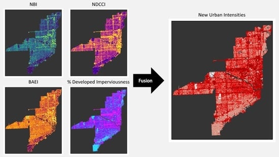
3.3. New Urban Intensities Derived from the Normalized Difference Concrete Condition Index
Building on the measurements achieved with NBI and BAEI, enhancements can be composited into a stack that could be utilized for the creation of discrete urban classes [27]. Miami’s urban fabric is rendered with NDCCI as a pronounced network of streets within open space, residential, and business areas. An effective enhancement composite would emphasize differences that exist between features within an urban landscape, where NBI, BAEI, and NDCCI do not yield similar renderings. Since NDVI is useful for identifying areas with or without vegetation, zonal statistics were calculated from urban land use types for both NDCCI and NDVI, both derived from the 2016 Landsat 8 data. NDCCI possesses less variation within classes, according to the coefficient of variation (CV) statistic, compared to NDVI (see Table 7). CV is calculated by dividing the standard deviation by the mean and may be written as a percentage; it gives a measure of the amount of statistical variation that exists between classes, allowing for direct comparison.
Iso cluster classifications for NDCCI/NBI/BAEI and NDVI/NBI/BAEI composites were created for visual comparison. Both composites were assigned arbitrary classes of Urban 1-5, yielding a view of development intensities based on respective enhancements. Areas in classes 1–3 are typically open space, vegetated, or residential, whereas areas of intense development are found in classes 4 and 5. The maps were compared for the clarity of discrete urban features. Examining the two maps in Figure 9, finer surface features such as Marlins Park, highways, and streets are more vividly rendered with the NDCCI/NBI/BAEI classification. The features in the NDVI/NBI/BAEI are comparatively saturated, with the compromise of less detail. Unsupervised classification can yields maps that, by themselves, may be valuable for the identification of specific surface features and for vectorizing those features into point, polygon, or line shapes. Therefore, further analysis was conducted with a supervised classifier to map the spatial configuration of Miami’s urban features more accurately.
3.3.1. Classifying Urban Intensities with Support Vector Machine
A supervised classification was created with the SVM classifier to build upon the unsupervised classification of the NDCCI/NBI/BAEI composite. Upon examining Figure 10a, it is clear that the SVM method identifies urban intensity in three simple classes and features corrections to class conflicts found in NLCD 2016. Zonal statistics were calculated for urban land use types to assess the accuracy of the classification. Referring to Table 8, Urban 1 is typified by recreation and other low intensity development, Urban 2 by residential areas, and Urban 3 by business and other high intensity development. Capitalizing on the spectral configuration initially identified for NBI in Section 3.1, highly developed areas are distinguished from open areas, clearly bordered by areas of mostly residential development. Where NLCD features an additional class to describe medium intensity, further analysis was conducted to fuse that class with the SVM classification to increase cartographic detail. The results infer this is a globally replicable method that can be replicated globally to provide urban area maps that describe development in three classes.
3.3.2. The Fusion Map
USGS classifies areas identified as possessing 50–79% impervious surface as medium intensity, and the class is rendered as a detail of streets and well-developed buildings in the NLCD classified product. The SVM classification reduced the errors related to feature structure found in NLCD 2016. In reciprocal, areas identified by USGS as medium intensity were conditionally geoprocessed to overlay the SVM classification as a new third class typified by moderate intensity business and medium-to-high intensity residential development, yielding classes Urban 1–4 (see Figure 10b,c). Upon visual inspection, it was discerned that some well-developed features, such as Marlins Park, may still be classified incorrectly into lower classes after fusing the SVM classification with the NLCD percent developed imperviousness data. To correct those features, the fifth class of the unsupervised NDCCI/NBI/BAEI classification was overlaid as a new class. Upon subsequent visual inspection, the result of adding this fifth class was a successful fusion. the brightest features, such as Marlins Park, freeways, and high intensity industrial and commercial development were classified as Urban 5. By decomposing the fifth class into the fourth, a new four-class urban intensity map without the pronounced errors of NLCD 2016 was created. The five-class fusion map does much to divide areas of the highest intensity from the fourth class, and the visualization may possess an aesthetic appeal. The four-class fusion map is more homogenous compared to NLCD 2016, having classification errors associated with urban intensities derived only from the percent developed imperviousness corrected (see Figure 10d–f).
Zonal statistics were calculated for the NLCD 2016 Miami urban intensities as well as the NDCCI/NBI/BAEI five-class and four-class fusion maps. Improvements were made in the fusion classifications (see Table 9). For example, NLCD 2016 open space is typified by both open areas and urban canopy, and the refined fusion classification effectively separates open areas from the urban canopy. The distribution of urban intensity classes among land use types is similar between the four-class maps. However, NLCD 2016 shows a large amount of residential areas classified incorrectly in the first class and noticeably less area in the fourth class. Based on the results, it can be concluded this is an effective methodology for producing urban intensity maps that correctly delineate detailed stages of development according to enhanced reflectance retrieved from a remote sensor. It is proposed that the process of classifying urban intensity with a satellite image in this analysis is effective for creating cartographic products of urban intensity that are superior to those currently found in NLCD.
Having established mapping conventions with NBI, BAEI, and NDCCI, further consideration was given to the potential for establishing an infill urban growth prediction implementing well-known land change geosimulation modeling methodology based on the unexplored potential of utilizing BAEI as a shadow index.
3.4. Geosimulating High-Rise Infrastructure Development
A time-series of BAEI rasters without feature extraction thresholding, including data from Landsat 5 for 2003 and 2008 and Landsat 8 for 2016, clipped to the Brickell neighborhood, captures the formation of shadows (see Figure 11a–c). Additional clipping was performed to isolate an area of interest (see Figure 11d–f). By focalizing the rasters to a one-cell radius circle, the shadows were grouped into simple circular features in a new raster, and a threshold that set a good visible fit for highlighting the shadows seen in the BAEI images was applied. Simple four-class land use maps, compatible with the LCM module, were created for the 2003 and 2008 data through the manual interpretation of high-resolution 2016 basemap imagery available through ArcGIS and geoprocessing to include the shadows. Before initiating the geosimulation, polynomial transition trends were mapped within LCM during the module’s model fitting routine to determine a series of polynomial transition trends that could serve as effective predictors of the transition from “business” to “high-rise shadow” (see Figure 12).
The assumption made was that the geosimulation need not predict the 2016 focalization exactly and that the prediction will, at least, closely outline the area where new high-rise infrastructure has been constructed. LCM features an accuracy assessment tool that will accept a classification map as input, though the results of this analysis were left to visual assessment. The output raster was clipped to the area of interest and vectorized. Figure 13 displays the geosimulation output as two maps: the predicted land use classification for the area of interest and a simplified vector of the output classified as shadows. The predicted vector, referencing the 2016 data, provides an excellent visual fit for the shadows rendered with BAEI. It is proposed that this is a novel method for predicting the formation of skyscrapers based on the reasonable fit of the projected vector. This analysis serves as a basic example of effective modeling that can be achieved through the proper model fitting of a geosimulation that performs based on the classification of urban land use according to transition potentials.
4. Discussion
Jieli et al. (2010) [14] developed NBI to enhance the scale of the brightness of urban features in a satellite image. Value ranges for this index, calculated from 2016 Landsat 8 data, are found to be descriptive of discrete land use types, according to feature brightness. Objects capturing the shapes of Miami’s urban feature types were visualized, and an object delineating an isolated formation of industrial land was successfully extracted. It is proposed that NBI is a utility for feature extraction of urban land use types through OBIA. Then, building upon the potential for identifying discrete urban land use types, the possibility of grading urbanization in terms of collective development was investigated. Bouzekri et al. (2015) [12] developed BAEI to enhance the brightness of urban features in a satellite image. Time-series analyses of Miami visualized with this index, spanning 1985–2016, yields a view of linear increase. Also, the success of a nine image time-series analysis comparing the two indices for the truncated area was successful in identifying a negative correlation between them. It is proposed that BAEI can be utilized during urban surface quality analyses to describe the upward scale of development. Samsudin et al. (2016) [20] developed NDCCI to enhance the presence and condition of construction material. Therefore, despite similar spectral configurations, it was suggested that this index might be more useful for urban mapping than NDVI, which is designed to enhance the presence and condition of vegetation. A comparison between the two indices, derived from 2016 Landsat 8 data, with FGDL Miami land use data found NDCCI possesses less within-class variance compared to NDVI. A visual comparison of iso cluster classifications of NDCCI/NBI/BAEI and NDVI/NBI/BAEI composites showed the NDCCI composite rendered Miami with less saturation between features of various intensity.
Furthermore, it was discernable that urbanization can be linearly rendered according to three dominant feature types: open space, residential, and business/transport areas. Therefore, SVM was used to classify the NDCCI composite in three stages of intensity based on training samples decided from a comparison between the composite and 2016 high-resolution satellite imagery. In addition to functioning as a standalone method, it serves as a palette for more detailed cartographic analyses to maximize the amount of information extracted from satellite data. It was possible to add more detail by fusing the SVM classification with NLCD 2016 percent developed imperviousness data. The area of Miami classified in NLCD 2016 as medium intensity was fused with the SVM classification in addition to the fifth class of the NDCCI composite iso cluster classification to correct any residual errors. Because of the simple workflow, it is within reason to assert the proposed methodology, when rigorously applied, may facilitate the production of maps on any scale.
There is global consideration for the use of LULC maps, such as those created during this research, as inputs into predictive geosimulations [1,2,3]. For example, Sun et al. (2007) [1] simulate the internal growth of Calgary, Alberta, Canada utilizing discrete classes derived from city land use data. Object maps derived from NBI may be implemented to facilitate this type of geostatistical modeling. In this study, BAEI rasters without feature extraction thresholds were focalized to magnify the presence of detected high-rise shadows in Miami’s Brickell neighborhood. Classifications derived from manual interpretation and focal analysis of 2003 and 2008 Landsat 5 data were used as inputs for an MLP ANN Markov Chain geosimulation, as well as polynomial transition trends derived from the classifications for predictors. The geosimulation generated a land use prediction that closely circled the formation of high-rise shadows in 2016 Landsat 8 data. The proposed methodology may be replicated to predict the formation of any relevant discrete occurrence that may be otherwise difficult to predict, given the isolated nature of the occurrence. Additional model fitting may be useful in refining the prediction, such as the implementation of other predictor gradients.
Challenges for replicating the study methods include the availability of GIS and remote sensing data, evaluating OBIA settings, managing the presence of vegetation, fitting an iso cluster classification to suitably capture the intensity of features, establishment of correct SVM training samples, and establishing a geosimulation area of interest. While the static NBI, BAEI, composite iso cluster, and composite SVM maps can be generated globally, it is understood that the fusion maps can only be generated if a percent developed imperviousness product exists for the area being mapped. For the study area of Miami, the spectral response among built-up indices was found to be sensitive to differences between land use types and to changes that occurred over a time-series. It must be duly noted that the study area was found to be comprised of three primary types: open spaces, residential, and commercial development. The observable sensitivity may be attributed to the composition of the city’s morphology as well as lighting conditions attributed to the city’s position and the time of data acquisition. Henceforward future work must consider the sensitivity of spectral responses in urban areas with morphological compositions that differ from Miami, as well as the influence of differing lighting conditions.
5. Conclusions
Rapid urbanization stimulates a high demand for static mapping and geosimulations to support legislative and planning purposes. A caveat exists where LULC maps should be synthesized through a process of maximizing the amount of information that can be acquired from a satellite image. While this is not the first study to research the potential for incorporating spectral enhancements in classification processes delineating multiple states of urbanization, the paper systematically summarizes specific approaches to various aspects of urban analysis. It discusses the advantages and limitations of existing indices. The power of remote sensing and GIS were coupled to conceptualize new urban land use classification capabilities utilizing the NBI, BAEI, and NDCCI spectral enhancements. LULC maps generated without the details that may be acquired from these enhancements may be less useful in application.
Today, the trend of global urbanization has negatively impacted Earth by triggering climate change, lowering water quality, and reducing natural landscape, among other problems. In response, there is an increased need for frequently updated LULC maps, and smart growth policies have been implemented by those responsible for managing the development of cityscapes. The principle of infill development, the redevelopment of land within a cityscape, will become more important because of the goal of smart growth policies to build compact, high population urban areas instead of sprawling outward. When combined with the analytical capabilities of GIS, remote sensing data may be refined to focus on a specific geography. Miami, a city that exists in a sensitive coastal environment, continues to grow at a rapid pace. We should consider using the city as a study area for research on urban geographic information science. Maps derived from this research may be advantageous for strengthening all purposes that rely on LULC maps.
Significant to this study, NBI was demonstrated to possess the unique property of identifying discrete urban land use types as segmented objects. Urban LULC maps may be created, through the process of OBIA, based on the geometric configuration of discrete land use types rendered with NBI. BAEI was successfully implemented to visualize and scale the growth of an entire city as well as an area truncated of urban canopy. Such a rendering of urban surface quality may be useful for important tasks such as predicting stages of development bordering natural areas, where intense development may be detrimental to the environment. NDCCI, when composited with NBI and BAEI, can be utilized to classify stages of urban intensity effectively.
The development of urban growth geosimulation models meant to bolster management efforts may become the research frontier for all efforts to mitigate human-driven environmental impacts. Satellite data are generated continuously and serve as an excellent basis for the LULC maps necessary for geosimulations to operate. The urban land use classification methods introduced in this paper have the potential to serve as inputs into urban growth geosimulations. NBI can be used to extract predictable geometries, BAEI can be reclassified into value ranges describing predictable gradient development, and the NDCCI/NBI/BAEI composite maps can be used to facilitate predictions of fluctuating urban intensity. While it is beyond the scope of this paper to give further consideration to these ideas, the novel method incorporating the BAEI as a shadow index is a clear example of the type of geostatistical model that can be created to monitor a city’s internal growth. Forward, it should also serve as a primary example of the type of success that may be gleaned from focalized geosimulation models in general.
Author Contributions
P.L. developed methodology, performed formal analysis, validation, visualization, interpreted results and wrote the paper; L.B. and E.H. aided to methodological design and contributed to final manuscript. All authors have read and agreed to the published version of the manuscript.
Funding
This research received no external funding.
Acknowledgments
The authors thank San Francisco State University Department of Geography & Environment for time allowed to complete this manuscript. We thank all reviewers for their comments towards improving this manuscript.
Conflicts of Interest
The authors declare no conflict of interest.
References
- Sun, H.; Forsythe, W.; Waters, N. Modeling Urban Land Use Change and Urban Sprawl: Calgary, Alberta, Canada. Netw. Spat. Econ. 2007, 7, 353–376. [Google Scholar] [CrossRef]
- Guan, D.; Li, H.; Inohae, T.; Su, W.; Nagaie, T.; Hokao, K. Modeling urban land use change by the integration of cellular automaton and Markov model. Eco. Mod. 2011, 222, 3761–3772. [Google Scholar] [CrossRef]
- Rahimi, A.A. A methodological approach to urban land-use change modeling using infill development pattern—A case study in Tabriz, Iran. Ecol. Process. 2016, 5, 1–15. [Google Scholar] [CrossRef] [Green Version]
- Seto, K.C.; Güneralp, B.; Hutyra, L.R. Global forecasts of urban expansion to 2030 and direct impacts on biodiversity and carbon pools. Proc. Nat. Acad. Sci. USA 2012, 109, 16083–16088. [Google Scholar] [CrossRef] [Green Version]
- Mohan, M.; Kandya, A. Impact of Urbanization and Land-use/Land-cover Change on Diurnal Temperature Range: A Case Study of Tropical Urban Airshed of India Using Remote Sensing Data. Sci. Total Environ. 2015, 506–507, 453–465. [Google Scholar] [CrossRef] [PubMed]
- Nelson, K.C.; Palmer, M.A.; Pizzuto, J.E.; Moglen, G.E.; Angermeier, P.L.; Hilderbrand, R.H.; Dettinger, M.; Hayhoe, K. Forecasting the combined effects of urbanization and climate change on stream ecosystems: From impacts to management options. J. App. Ecol. 2009, 46, 154–163. [Google Scholar] [CrossRef] [PubMed] [Green Version]
- Zia, S.; Shirazi, S.A.; Bhalli, M.N.; Kausar, S. The impact of urbanization on mean annual temperature of lahore metropolitan area, pakistan. Pak. J. Sci. 2015, 67, 301–307. [Google Scholar]
- Han, G.; Xu, J. Land Surface Phenology and Land Surface Temperature Changes Along an Urban-Rural Gradient in Yangtze River Delta, China. Environ. Manag. 2013, 52, 234–249. [Google Scholar] [CrossRef] [PubMed]
- Pei, F.; Wu, C.; Liu, X.; Li, X.; Yang, K.; Zhou, Y.; Wang, K.; Xu, L.; Xia, G. Monitoring the vegetation activity in China using vegetation health indices. Agric. For. Meteorol. 2018, 248, 215–227. [Google Scholar] [CrossRef]
- Tang, H.; Li, Z.; Zhu, Z.; Chen, B.; Zhang, B.; Xin, X. Variability and Climate Change Trend in Vegetation Phenology of Recent Decades in the Greater Khingan Mountain Area, Northeastern China. Remote Sens. 2015, 7, 11914–11932. [Google Scholar] [CrossRef] [Green Version]
- As-syakur, A.; Adnyana, I.; Arthana, I.; Nuarsa, I. Enhanced Built-up and Bareness Index (EBBI) for Mapping Built-up and Bare Land in an Urban Area. Remote Sens. 2012, 4, 2957–2970. [Google Scholar] [CrossRef] [Green Version]
- Bouzekri, S.; Lasbet, A.; Lachehab, A. A New Spectral Index for Extraction of Built-up Area Using Landsat-8 Data. J. Indian Soc. Remote Sens. 2015, 43, 867–873. [Google Scholar] [CrossRef]
- He, C.; Shi, P.; Xie, D.; Zhao, Y. Improving the normalized difference built-up index to map urban built-up areas using a semiautomatic segmentation approach. Remote Sens. Lett. 2010, 1, 213–221. [Google Scholar] [CrossRef] [Green Version]
- Jieli, C.; Manchun, L.; Yongxue, L.; Chenglei, S.; Wei, H. Extract residential areas automatically by New Built-up Index. In Proceedings of the 2010 18th International Conference on Geoinformatics, Beijing, China, 18–20 June 2010; Volume 1. [Google Scholar]
- Rasul, A.; Balzter, H.; Ibrahim, G.R.F.; Hameed, H.M.; Wheeler, J.; Adamu, B.; Ibrahim, S.; Najmaddin, P.M. Applying Built-up and Bare-Soil Indices from Landsat 8 to Cities in Dry Climates. Land 2018, 7, 81. [Google Scholar] [CrossRef] [Green Version]
- Waqar, M.M.; Mirza, J.F.; Mumtaz, R.; Hussain, E. Development of new indices for extraction of built-up area and bare soil from landsat. Open Access Sci. Rep. 2012, 1, 1–4. [Google Scholar]
- Xu, H. A new index for delineating built-up land features in satellite imagery. Int. J. Remote Sens. 2008, 29, 4269–4276. [Google Scholar] [CrossRef]
- Zha, Y.; Gao, J.; Ni, S. Use of normalized difference built-up index in automatically mapping urban areas from TM imagery. Int. J. Remote Sens. 2003, 24, 583–594. [Google Scholar] [CrossRef]
- Benkouider, F.; Abdellaoui, A.; Hamami, L. New and Improved Built-up Index Using SPOT Imagery: Application to an Arid Zone (Laghouat and M’Sila, Algeria). J. Indian Soc. Remote Sens. 2019, 47, 185–192. [Google Scholar] [CrossRef]
- Samsudin, S.H.; Shafri, H.Z.M.; Hamedianfar, A. Development of spectral indices for roofing material condition status detection using field spectroscopy and WorldView-3 data. J. Appl. Remote Sens. 2016, 10, 025021. [Google Scholar] [CrossRef]
- Gu, L.; Cao, Q.; Ren, R. Building extraction method based on the spectral index for high-resolution remote sensing images over urban areas. J. Appl. Remote Sens. 2018, 12, 1. [Google Scholar] [CrossRef]
- Peeroo, U.; Idrees, M.; Saeidi, V. Building extraction for 3D city modelling using airborne laser scanning data and high-resolution aerial photo. S. Afr. J. Geomat. 2017, 6, 363–376. [Google Scholar] [CrossRef] [Green Version]
- United Nations Department of Economic and Social Affairs (UN DESA): World Population Projected to Reach 9.8 Billion in 2050, and 11.2 Billion in 2100. Available online: https://www.un.org/development/desa/en/news/population/world-population-prospects-2017.html (accessed on 15 December 2019).
- Abbas, A.W.; Ahmad, N.; Abid, S.A.R.; Khan, M.A.A. K-means and ISODATA Clustering Algorithms for Landcover Classification Using Remote Sensing. Sindh Univ. Res. J. SURJ (Sci. Ser.) 2016, 48, 315–318. [Google Scholar]
- Igun, E. Analysis and Sustainable Management of Urban Growth’s Impact on Land Surface Temperature in Lagos, Nigeria. J. Remote Sens. GIS 2017, 6, 212. [Google Scholar] [CrossRef]
- Pal, M.; Mather, P. Support vector machines for classification in remote sensing. Int. J. Remote Sens. 2005, 26, 1007–1011. [Google Scholar] [CrossRef]
- Ettehadi, O.E.; Kaya, S.; Elif, S.; Alganci, U. Separating Built-up Areas from Bare Land in Mediterranean Cities Using Sentinel-2A Imagery. Remote Sens. 2019, 11, 345. [Google Scholar] [CrossRef] [Green Version]
- Cabral, P. Délimitation d‘aires urbaines à partir d‘une image Landsat ETM+: Comparaison de méthodes de classification. Can. J. Remote Sens. 2007, 33, 422–430. [Google Scholar] [CrossRef]
- Beck, L.; Hutchinson, R.; Zauderer, C. A comparison of greenness measures in two semi-arid grasslands. Clim. Chang. 1990, 17, 287–303. [Google Scholar] [CrossRef]
- Jin, S.; Homer, C.; Yang, L.; Danielson, P.; Dewitz, J.; Li, C.; Zhu, Z.; Xian, G.; Howard, D. Overall Methodology Design for the United States National Land Cover Database 2016 Products. Remote Sens. 2019, 11, 2971. [Google Scholar] [CrossRef] [Green Version]
- Environmental Systems Research. ArcGIS Pro: Version 2.5.1; Environmental Systems Research Institute (ESRI): Redlands, CA, USA, 2020. [Google Scholar]
- Hexagon Geospatial. ERDAS Imagine: Version 16.5.0; Hexagon Geospatial: Madison, AL, USA, 2018. [Google Scholar]
- Clark Labs, Clark University. TerrSet Geospatial Monitoring and Modeling Software: Version 18; Clark Labs, Clark University: Worcester, MA, USA, 2015. [Google Scholar]
- World Population Review: Miami, Florida Population 2020. Available online: http://worldpopulationreview.com/us-cities/miami-population/ (accessed on 12 April 2020).
- Kim, J.; Steiner, R.; Yang, Y. The Evolution of Transportation Concurrency and Urban Development Pattern in Miami-Dade County, Florida. Urban Aff. Rev. 2014, 50, 672–701. [Google Scholar] [CrossRef]
- United States Geological Survey (USGS): Landsat Surface Reflectance. Available online: https://www.usgs.gov/land-resources/nli/landsat/landsat-surface-reflectance (accessed on 12 April 2020).
- Phiri, D.; Morgenroth, J. Developments in Landsat Land Cover Classification Methods: A Review. Remote Sens. 2017, 9, 967. [Google Scholar] [CrossRef] [Green Version]
- Chrysoulakis, N. Estimation of the all-wave urban surface radiation balance by use of ASTER multispectral imagery and in situ spatial data. J. Geophys. Res. Atmos. 2003, 108. [Google Scholar] [CrossRef] [Green Version]
- Dixit, A.; Goswami, A.; Jain, S. Development and Evaluation of a New “Snow Water Index (SWI)” for Accurate Snow Cover Delineation. Remote Sens. 2019, 11, 2774. [Google Scholar] [CrossRef] [Green Version]
- Hochmair, H.H.; Gann, D.; Benjamin, A.; Fu, J. Miami-Dade County Urban Tree Canopy Assessment; GIS Center, Florida International University: Miami, FL, USA, 2016. [Google Scholar]
- Ball, G.H.; Hall, D.J. Isodata: A Method of Data Analysis and Pattern Classification; Stanford University: Menlo Park, CA, USA, 1965. [Google Scholar]
- Cortes, C.; Vapnik, V. Support-vector Networks. Mach. Learn. 1995, 20, 273–297. [Google Scholar] [CrossRef]
- Ustuner, M.; Sanli, F.B.; Abdikan, S. Balanced vs imbalanced training data: Classifying rapideye data with support vector machines. Int. Arch. Photogramm. Remote Sens. Spat. Inf. Sci. 2016, XLI-B7, 379–384. [Google Scholar] [CrossRef]
- Chen, D.; Stow, D. The Effect of Training Strategies on Supervised Classification at Different Spatial Resolutions. Photogramm. Eng. Remote Sens. 2002, 68, 1155–1161. [Google Scholar]
- Marius, P.; Balas, V.; Perescu-Popescu, L.; Mastorakis, N. Multilayer Perceptron and Neural Networks. WSEAS Trans. Circuits Syst. 2009, 8, 579–588. [Google Scholar]
Figure 1.
Miami sits on the southeastern tip of Florida. The city is enclosed by Biscayne Bay and the Atlantic Ocean to the east, and urbanized parts of Miami-Dade County inland.
Figure 1.
Miami sits on the southeastern tip of Florida. The city is enclosed by Biscayne Bay and the Atlantic Ocean to the east, and urbanized parts of Miami-Dade County inland.

Figure 2.
Select spectral enhancements derived from Landsat 8 OLI 22 October 2016 data; (a) NBI, (b) BAEI, (c) NDCCI.
Figure 2.
Select spectral enhancements derived from Landsat 8 OLI 22 October 2016 data; (a) NBI, (b) BAEI, (c) NDCCI.

Figure 3.
USGS NLCD 2016 urban intensities with noticeable errors denoted.

Figure 4.
Urban intensity classification workflow diagram.

Figure 5.
NBI object primitives derived from Landsat 8 OLI 22 October 2016 data; (a) small segment size emphasizing surface brightness (spectral detail: 13, spatial detail: 8, minimum segment size in pixels: 1), (b) moderate segment size emphasizing surface objects (spectral detail: 15, spatial detail: 10, minimum segment size in pixels: 5), (c) large segment size emphasizing surface texture (spectral detail: 17, spatial detail: 12, minimum segment size in pixels: 10).

Figure 6.
NBI-derived object of industrialized land in Little Haiti.

Figure 7.
BAEI change detection time-series, giving mean index values, derived from Landsat data; (a) 5 TM 2 November 1985, (b) 6 November 1998, (c) 20 November 2003, (d) 10 November 2011, (e) 8 OLI 17 October 2014, (f) 22 October 2016.
Figure 7.
BAEI change detection time-series, giving mean index values, derived from Landsat data; (a) 5 TM 2 November 1985, (b) 6 November 1998, (c) 20 November 2003, (d) 10 November 2011, (e) 8 OLI 17 October 2014, (f) 22 October 2016.

Figure 8.
Change detection time-series, giving mean index values, derived from Landsat 5 TM data; (a) 2 November 1985 BAEI, (b) 6 November 1998 BAEI, (c) 10 November 2011 BAEI, (d) 2 November 1985 NDVI, (e) 6 November 1998 NDVI, (f) 10 November 2011 NDVI.
Figure 8.
Change detection time-series, giving mean index values, derived from Landsat 5 TM data; (a) 2 November 1985 BAEI, (b) 6 November 1998 BAEI, (c) 10 November 2011 BAEI, (d) 2 November 1985 NDVI, (e) 6 November 1998 NDVI, (f) 10 November 2011 NDVI.

Figure 9.
Iso cluster classifications of urban land use intensity based on spectral index composites derived from 22 October 2016 Landsat 8 OLI data; (a) NDCCI/NBI/BAEI composite, (b) NDVI/NBI/BAEI composite.
Figure 9.
Iso cluster classifications of urban land use intensity based on spectral index composites derived from 22 October 2016 Landsat 8 OLI data; (a) NDCCI/NBI/BAEI composite, (b) NDVI/NBI/BAEI composite.

Figure 10.
2016 Miami urban land use classifications derived from Landsat 8 OLI data; (a) NDCCI/NBI/BAEI composite SVM, (b) NLCD 2016 Percent Developed Imperviousness, (c) fusion of NDCCI/NBI/BAEI SVM and Percent Developed Imperviousness, (d) NDCCI/NBI/BAEI composite iso cluster, (e) five-class fusion of Percent Developed Imperviousness with NDCCI/NBI/BAEI SVM and iso cluster, (f) four-class fusion of Percent Developed Imperviousness with NDCCI/NBI/BAEI SVM and iso cluster.

Figure 11.
BAEI (as a shadow index) change detection time-series of the Brickell neighborhood derived from Landsat data; (a) 5 TM 20 November 2003, (b) 17 November 2008, (c) 8 OLI 22 October 2016. The area of interest overlaid with a focalized classification (transparent) based on thresholding; (d) 5 TM 20 November 2003. (e) 17 November 2008. (f) 8 OLI 22 October 2016.

Figure 12.
Classifications, created by manual and semi-automated methods, of the Brickell neighborhood derived from Landsat 5 TM data used as LCM inputs; (a) 20 November 2003, (b) 17 November 2008. Polynomial transition trends created in LCM; (c) 2nd order, (d) 3rd order.
Figure 12.
Classifications, created by manual and semi-automated methods, of the Brickell neighborhood derived from Landsat 5 TM data used as LCM inputs; (a) 20 November 2003, (b) 17 November 2008. Polynomial transition trends created in LCM; (c) 2nd order, (d) 3rd order.

Figure 13.
Results of LCM 2016 prediction for Brickell neighborhood area of interest based on 2003 and 2008 data; (a) predicted 2016 area of interest land cover, (b) vector derived from 2016 prediction referencing the formation of shadows in the area of interest.
Figure 13.
Results of LCM 2016 prediction for Brickell neighborhood area of interest based on 2003 and 2008 data; (a) predicted 2016 area of interest land cover, (b) vector derived from 2016 prediction referencing the formation of shadows in the area of interest.


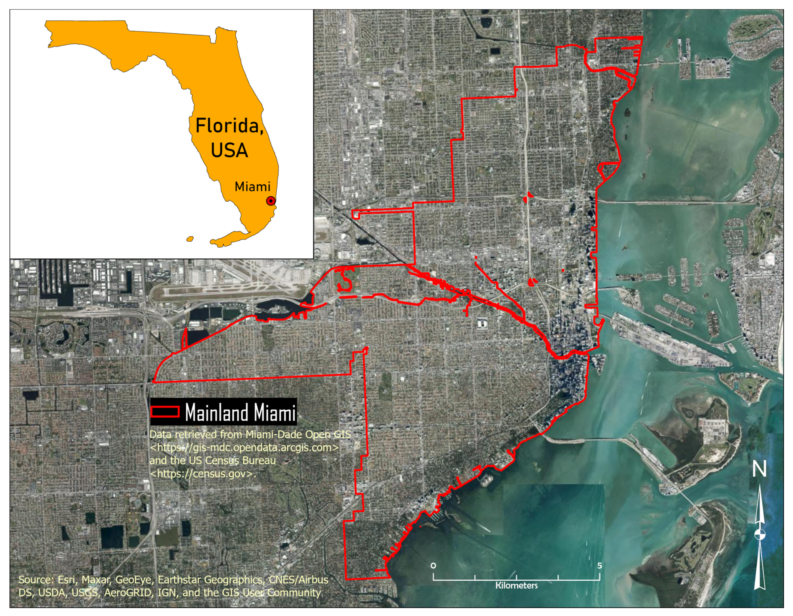
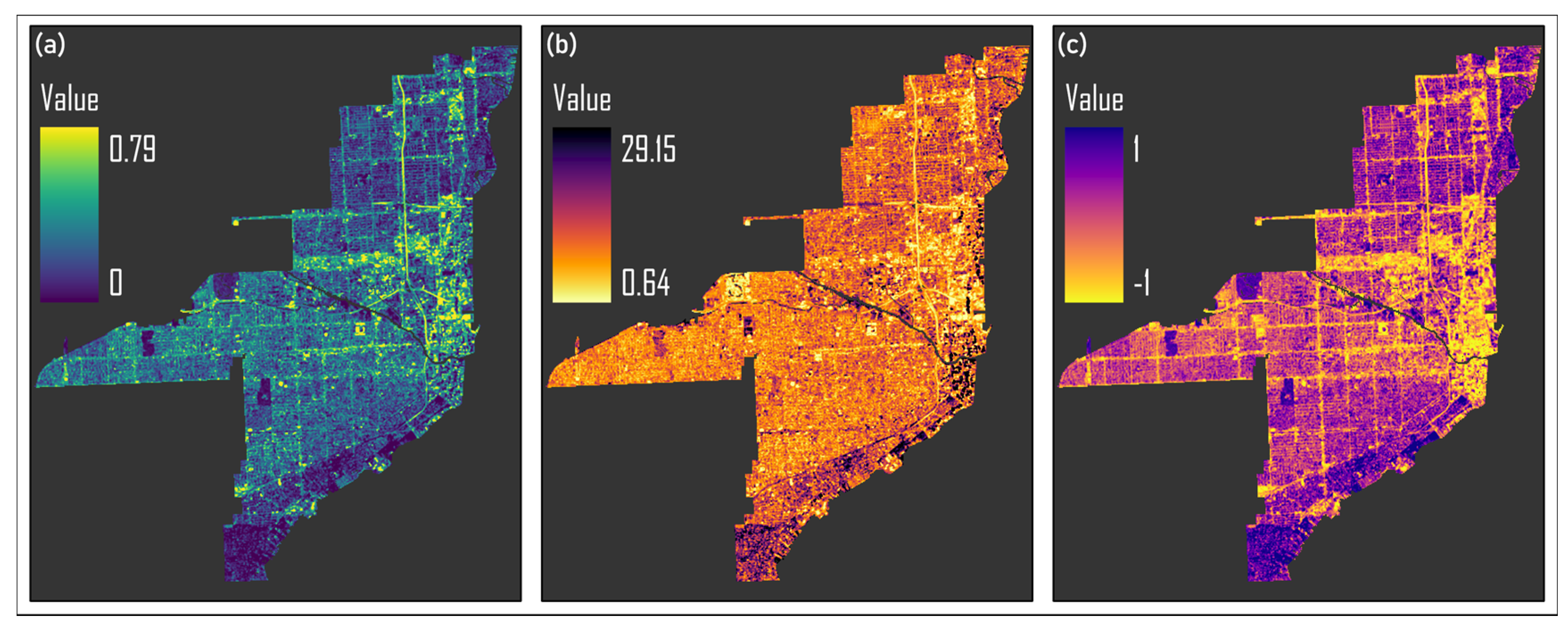
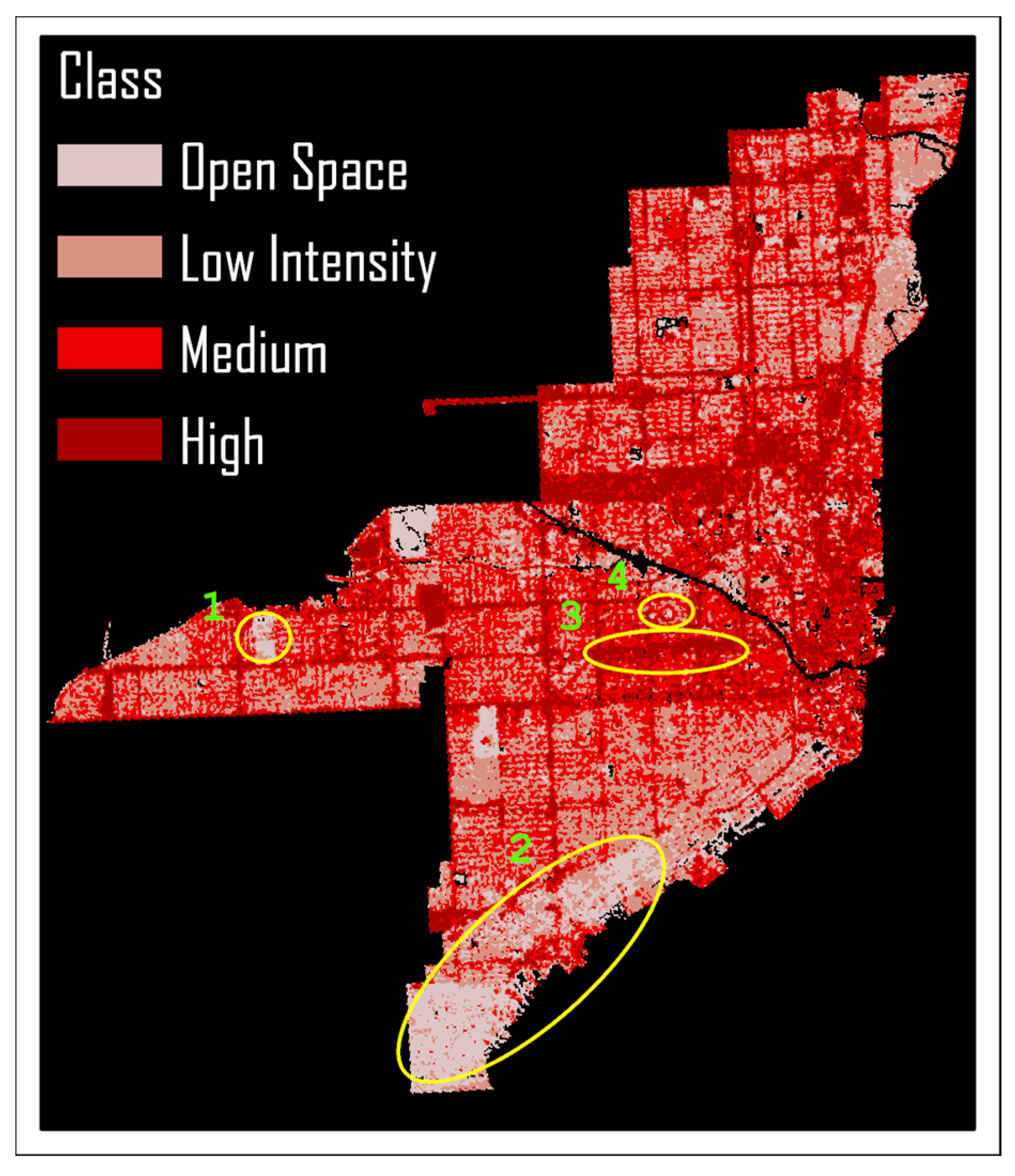
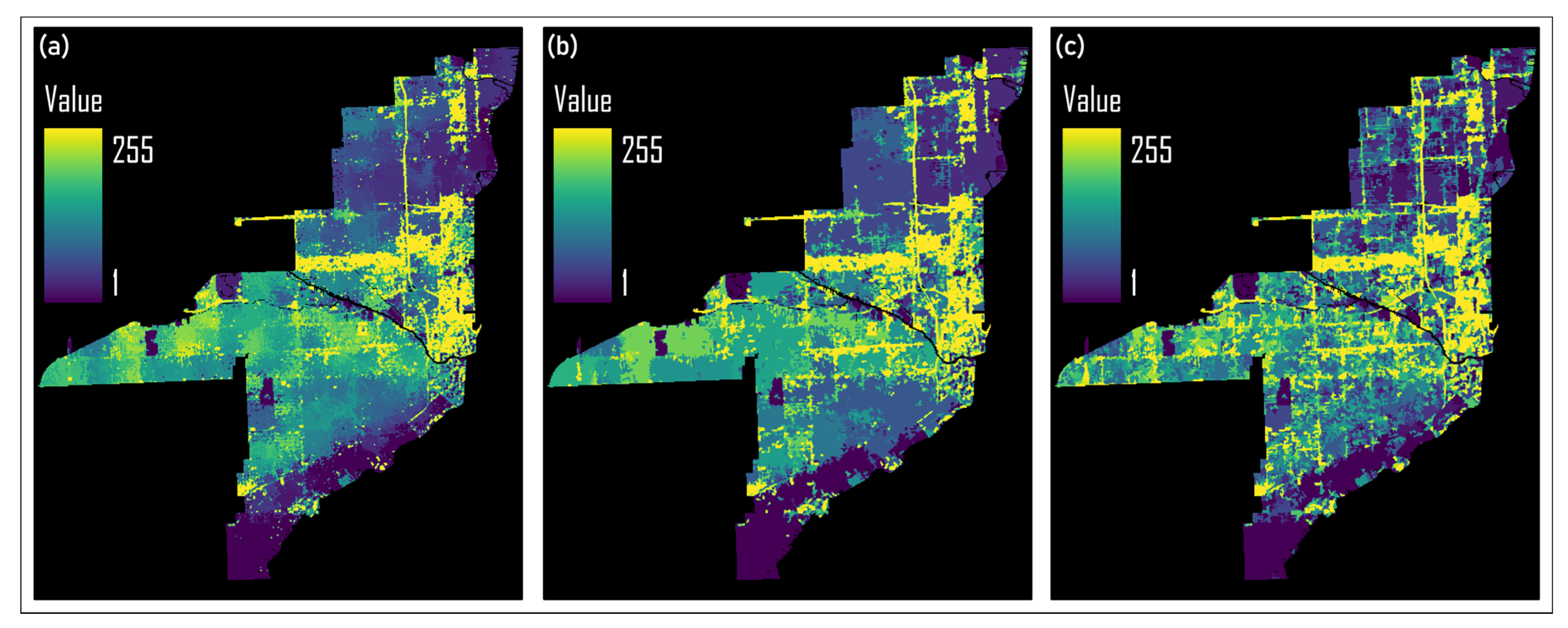
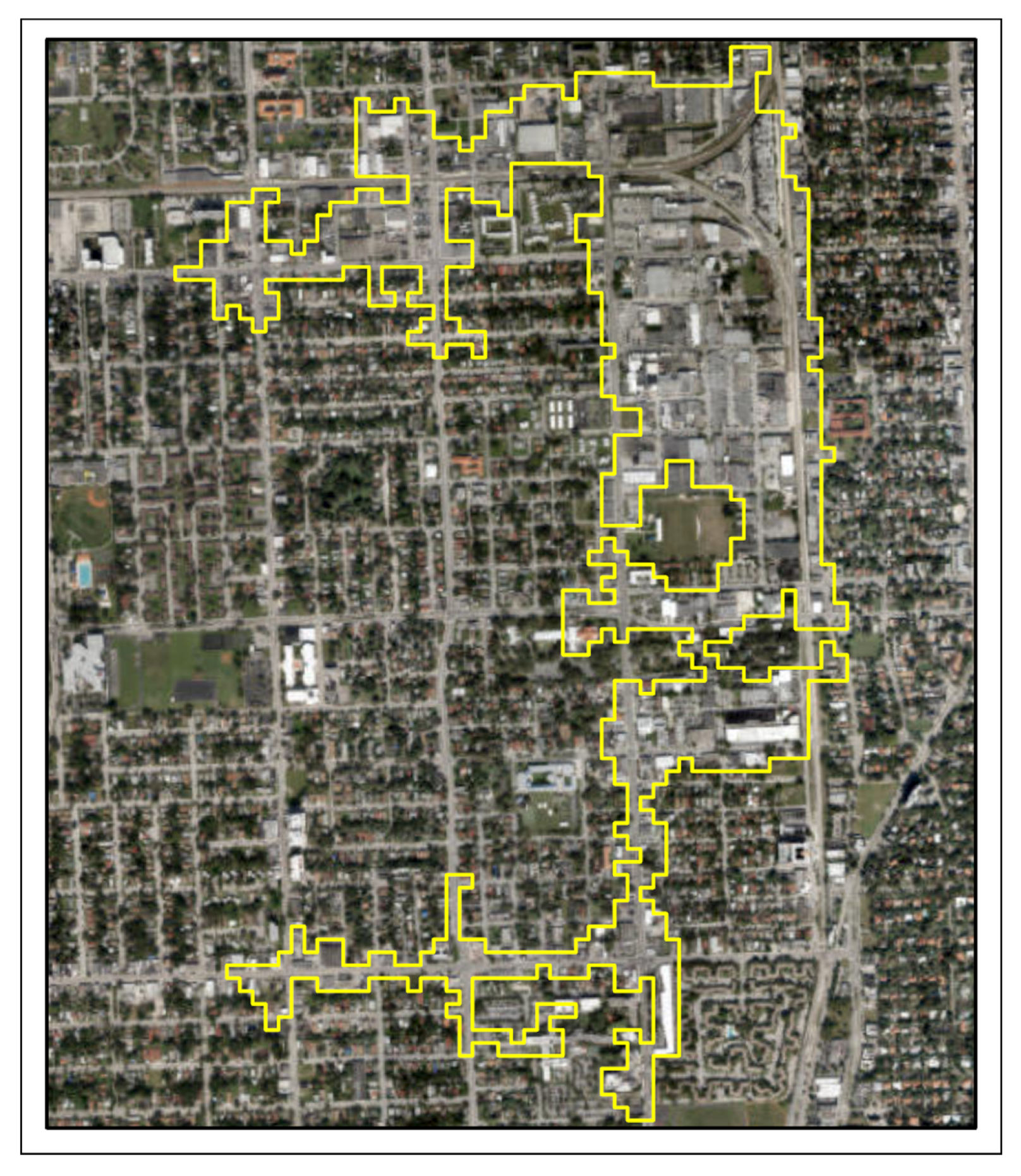
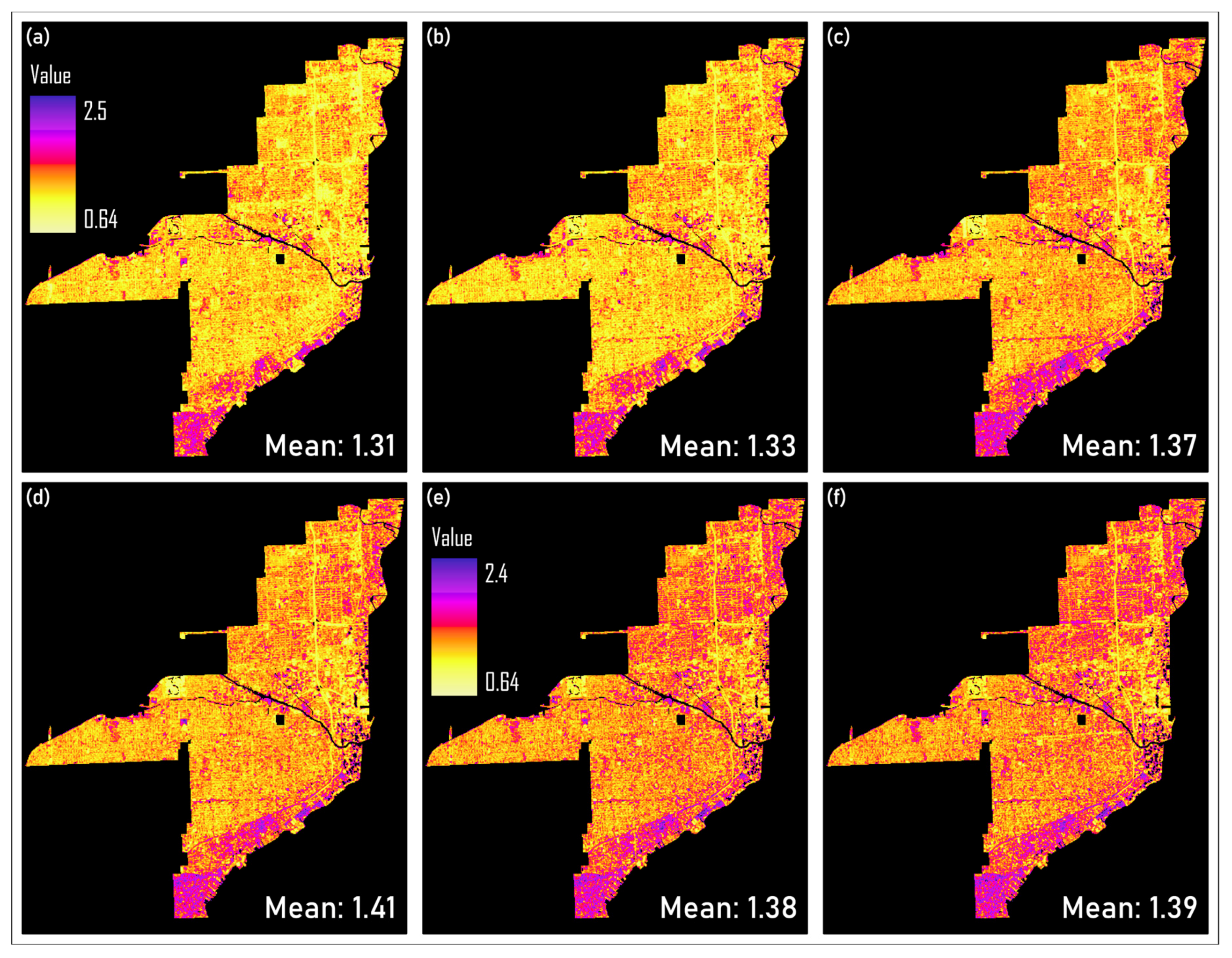
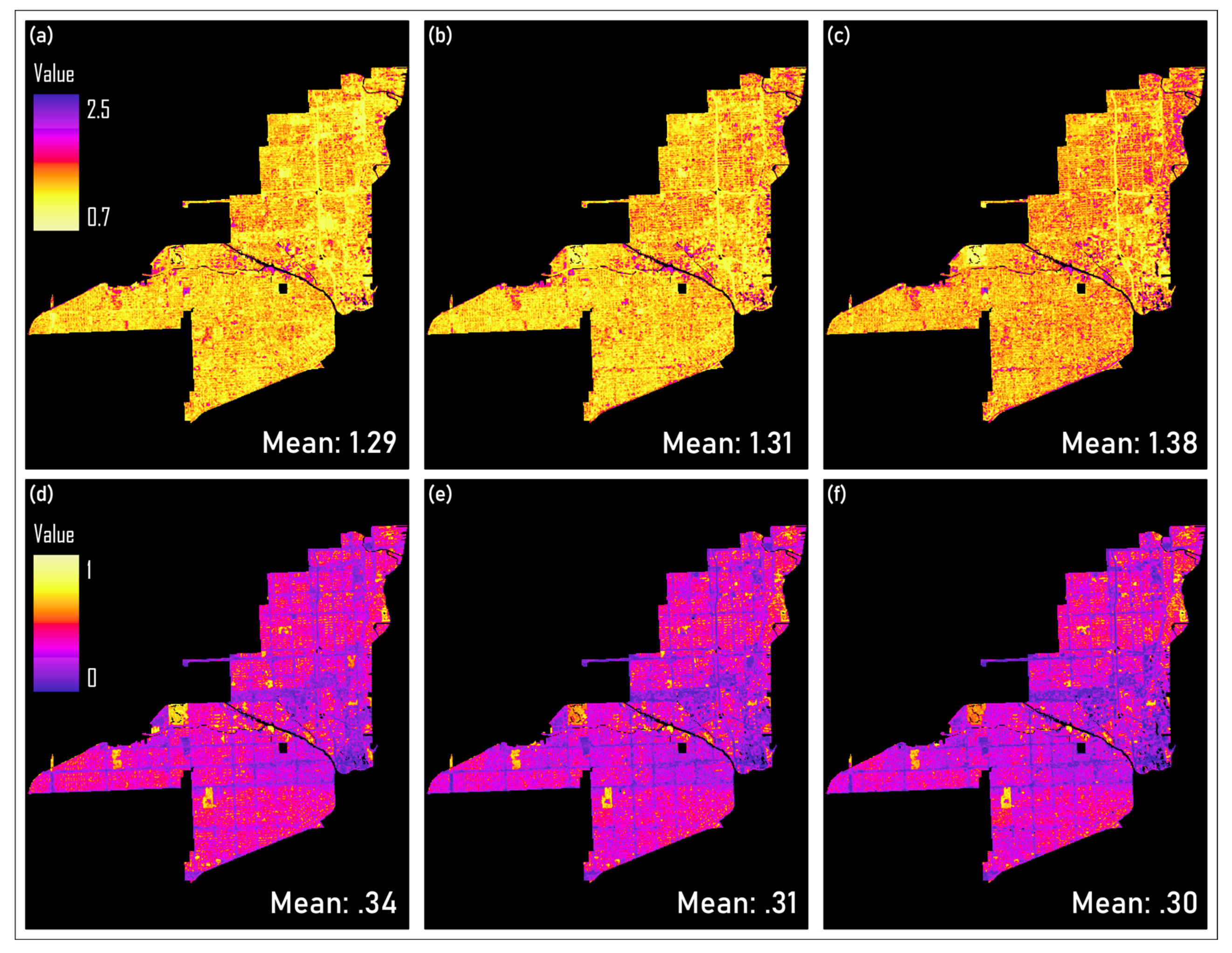
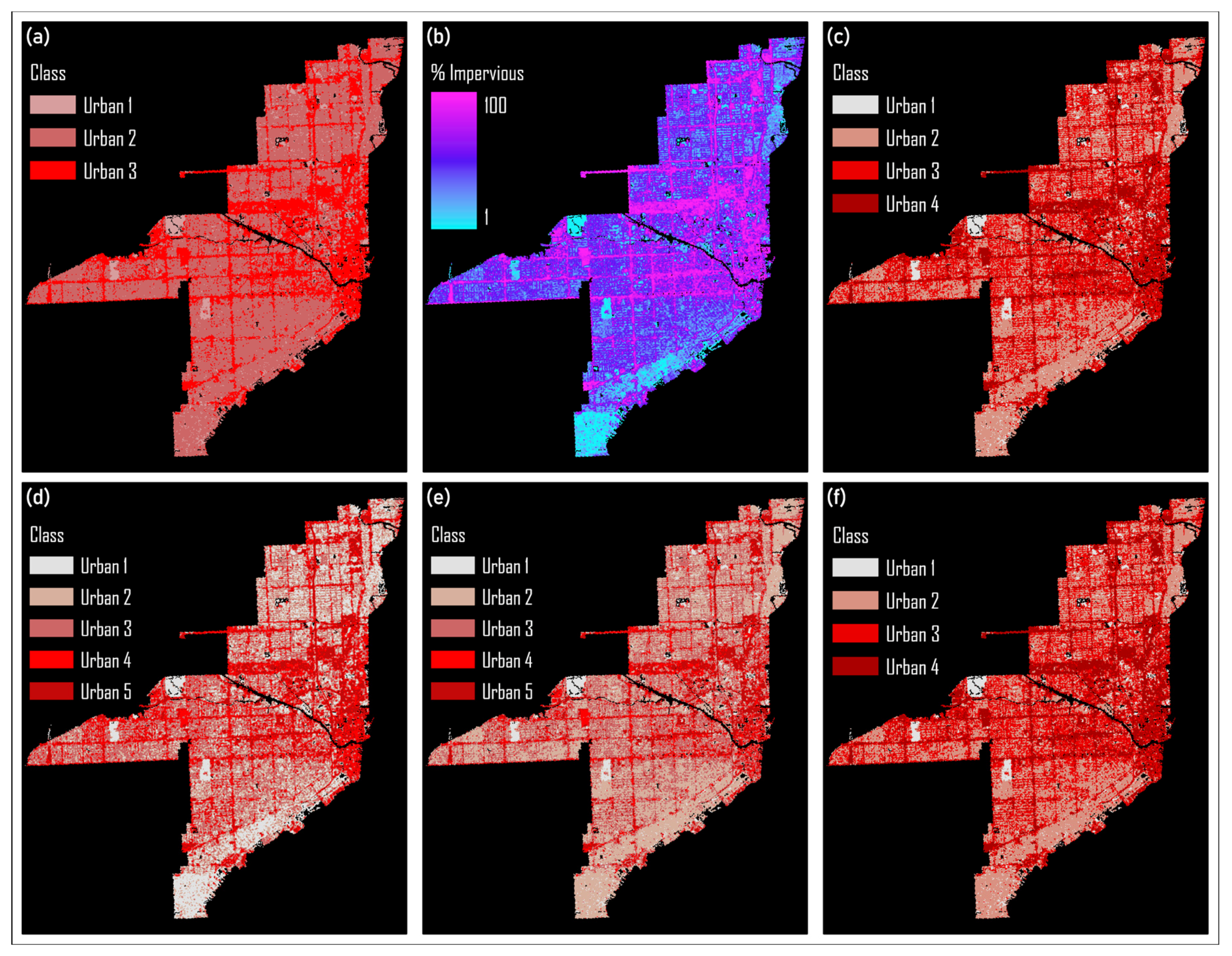
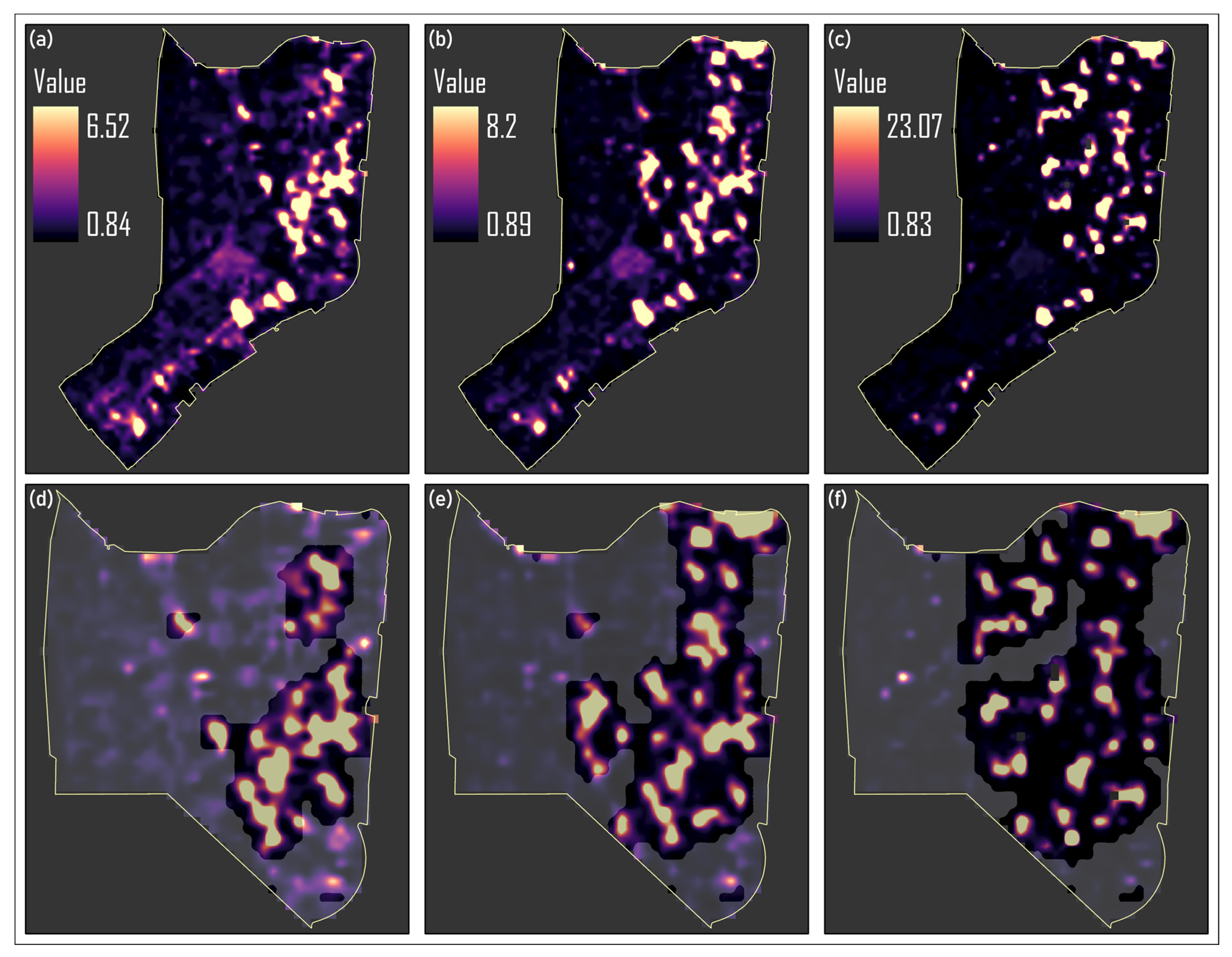
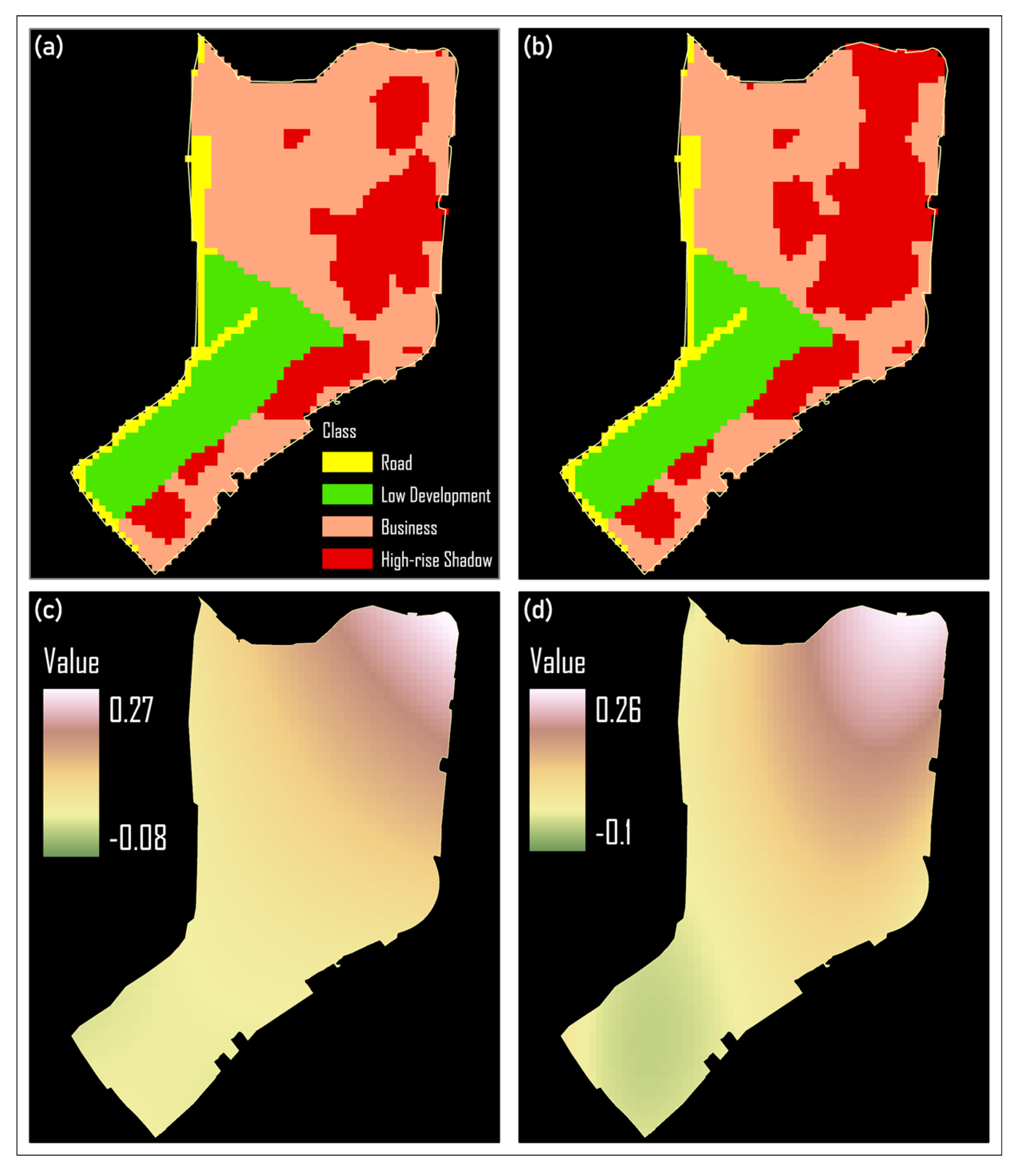
Table 1.
Inventory of all of the geospatial data used during this study, including descriptive information.
Table 1.
Inventory of all of the geospatial data used during this study, including descriptive information.
| GIS Data | |||
|---|---|---|---|
| Description | Year(s) | Source | Format |
| Miami-Dade Municipal Boundaries | 2018 | Miami-Dade Open GIS | Vector shapefiles |
| Miami-Dade Municipal Coastal Boundary | |||
| Miami-Dade Water Features | |||
| Florida Neighborhood Boundaries | 2018 | Zillow Real Estate Listings | |
| Generalized Land Use Derived from 2017 Parcels - Florida Department of Transportation District 6 | 2017 | Florida Geographic Data Library | Vector shapefiles (converted to raster images) |
| Statewide Land Use Land Cover | 2014–2016 | Florida Department of Environmental Protection Geospatial Open Data | |
| National Land Cover Database | 2016 | United States Geological Survey | Raster images |
| National Land Cover Database Percent Developed Imperviousness | |||
| Remote Sensing Data | |||
| Landsat Scene ID | Date | Cloud Cover | Sensor |
| LT05_L1TP_015042_19851102_20161004_01_T1 | 2 November 1985 | 0% | Landsat 5 TM |
| LT05_L1TP_015042_19981106_20160922_01_T1 | 6 November 1998 | 0% | |
| LT05_L1TP_015042_19991024_20160919_01_T1 | 24 October 1999 | 0% | |
| LT05_L1TP_015042_20031120_20160914_01_T1 | 20 November 2003 | 0% | |
| LT05_L1TP_015042_20081117_20160908_01_T1 | 17 November 2008 | 0% | |
| LT05_L1TP_015042_20091019_20160904_01_T1 | 19 October 2009 | 2% | |
| LT05_L1TP_015042_20111110_20160830_01_T1 | 2 November 2011 | 0% | |
| LC08_L1TP_015042_20141017_20170303_01_T1 | 17 October 2014 | 0.01% | Landsat 8 OLI |
| LC08_L1TP_015042_20161022_20170219_01_T1 | 22 October 16 | 0.08% | |
Table 2.
Built-up indices found in scientific journals evaluated for unique spectral properties.
| Name of Index | Author(s) | Formula | Accuracy | Study Area |
|---|---|---|---|---|
| The Enhanced Built-up and Bareness Index (EBBI) | As-syakur et al. (2012) [11] | (SWIR1−NIR)/10*SQRT (SWIR1+THERMAL) | 88.98% | Densapar, Indonesia |
| The Built-up Area Extraction Index (BAEI) | Bouzekri et al. (2015) [12] | (RED+0.3)/(GREEN+SWIR1) | 92.66% | Djelfa, Algeria |
| The Built-up Index (BUI) | He et al. (2010) [13] | (SWIR1−NIR)/(SWIR1+NIR)− (NIR−RED)/(NIR+RED) | 86.3% | National Olympic Park, Beijing, China |
| The New Built-up Index (NBI) | Jieli et al. (2010) [14] | (RED−SWIR1)/(NIR) | 90% | Changzhou City, China |
| The Dry Built-up Index (DBI) | Rasul et al. (2018) [15] | (BLUE−THERMAL)/(BLUE+THERMAL)− (NIR−RED)/(NIR+RED) | 93% | Erbil, Iraq |
| The Normalized Built-up Area Index (NBAI) | Waqar et al. (2012) [16] | [(SWIR2−SWIR1)/GREEN]/ [(SWIR2+SWIR1)/GREEN] | 86.87% | Islamabad, Pakistan |
| The Band Ratio for Built-up Area (BRBA) | (RED)/(SWIR1) | 85.09% | ||
| The Index-based Built-up Index (IBI) | Xu (2008) [17] | 2*SWIR1/(SWIR1+NIR)−[NIR/(NIR−RED)+ GREEN/(GREEN+SWIR1)]/ 2*SWIR1/(SWIR1+NIR)+ [NIR/(NIR−RED)+GREEN/ (GREEN+SWIR1)] | 96.77% | Fuzhou City, South China |
| The Normalized Difference Built-up Index (NDBI) | Zha et al. (2003) [18] | (SWIR1−NIR)/(SWIR1+NIR) | 92.6% | Nanjing City, East China |
| Index Designed for Extracting Urban Features from SPOT Data | ||||
| The Modified Built-up Area Index (MBAI) | Benkouider et al. (2019) [19] | [NIR+(1.57*GREEN)+(2.4*SWIR1)]/(1+NIR) | 95% & 91% | Laghouat and M’Sila, Algeria |
| Index Designed for Determining Material Condition from High-resolution Data | ||||
| The Normalized Difference Concrete Condition Index (NDCCI) | Samsudin et al. (2016) [20] | (NIR−GREEN)/(NIR+GREEN) | 84.44% | University Putra Malaysia, Seri Kembangan, Malaysia |
Table 3.
Breakdown of the number of training polygons and pixels sampled for each SVM class.
| Class | Polygons | Pixels |
|---|---|---|
| Urban 1 | 6 | 931 |
| Urban 2 | 9 | 3572 |
| Urban 3 | 9 | 1580 |
| Total | 24 | 6083 |
Table 4.
Zonal statistics of NBI derived from 22 October 2016 Landsat 8 OLI data, referencing FGDL data.
Table 4.
Zonal statistics of NBI derived from 22 October 2016 Landsat 8 OLI data, referencing FGDL data.
| Land Use | Area (sq km) | Min | Max | Range | Mean | Std |
|---|---|---|---|---|---|---|
| Centrally Assessed 1 | 0.33 | 0.0195 | 0.2788 | 0.2593 | 0.1262 | 0.0535 |
| Industrial | 1.97 | 0.0209 | 0.5135 | 0.4927 | 0.1698 | 0.0663 |
| Institutional 2 | 2.51 | 0.0002 | 0.4243 | 0.4241 | 0.0846 | 0.0639 |
| Public/Semi-public 3 | 7.99 | 0.0004 | 0.7474 | 0.7470 | 0.0931 | 0.0711 |
| Recreation | 0.6 | 0.0037 | 0.3645 | 0.3607 | 0.0631 | 0.0564 |
| Residential | 36.78 | 0.0004 | 0.4011 | 0.4008 | 0.0785 | 0.0421 |
| Retail/Office | 7.52 | 0.0044 | 0.7848 | 0.7804 | 0.1356 | 0.0701 |
| Vacant Non-residential | 2.61 | 0.0056 | 0.4932 | 0.4877 | 0.1120 | 0.0754 |
| Vacant Residential | 1.84 | 0.0035 | 0.2860 | 0.2825 | 0.0607 | 0.0449 |
1 Centrally assessed refers to, for instance, utilities. 2 Instutional refers to religious, educational, social, cultural, or healthcare. 3 Public/Semi-public refers to schools, governmental.
Table 5.
Area statistics of NBI-derived object, referencing FGDL data.
| Land Use | Area (sq km) |
|---|---|
| Centrally Assessed | 0.06 |
| Industrial | 0.43 |
| Institutional | 0.05 |
| Public/Semi-public | 0.04 |
| Residential | 0.03 |
| Retail/Office | 0.14 |
| Vacant Nonresidential | 0.05 |
Table 6.
Zonal statistics of BAEI and NDVI values derived from Landsat 5 TM (1985–2011) and 8 OLI data (2014 & 2016), referencing the truncated study area.
Table 6.
Zonal statistics of BAEI and NDVI values derived from Landsat 5 TM (1985–2011) and 8 OLI data (2014 & 2016), referencing the truncated study area.
| Year | Mean BAEI | Mean NDVI |
|---|---|---|
| 1985 | 1.283 | 0.3388 |
| 1998 | 1.304 | 0.3121 |
| 1999 | 1.284 | 0.3142 |
| 2003 | 1.332 | 0.3074 |
| 2008 | 1.364 | 0.2945 |
| 2009 | 1.299 | 0.2891 |
| 2011 | 1.377 | 0.3049 |
| 2014 | 1.353 | 0.3900 |
| 2016 | 1.367 | 0.3897 |
Table 7.
Zonal statistics of 22 October 2016 NDCCI and NDVI, referencing FGDL data.
| NDCCI | |||||||
|---|---|---|---|---|---|---|---|
| Land Use | Area (sq km) | Min | Max | Range | Mean | Std | CV |
| Centrally Assessed | 0.33 | 0.004 | 0.701 | 0.698 | 0.345 | 0.124 | 35.96% |
| Industrial | 1.97 | −0.100 | 0.649 | 0.749 | 0.221 | 0.106 | 47.96% |
| Institutional | 2.51 | −0.316 | 0.881 | 1.197 | 0.461 | 0.190 | 41.12% |
| Public/Semi-public | 7.99 | −0.136 | 0.914 | 1.050 | 0.439 | 0.189 | 42.93% |
| Recreation | 0.6 | −0.177 | 0.824 | 1.002 | 0.515 | 0.208 | 40.33% |
| Residential | 36.78 | −0.289 | 0.915 | 1.205 | 0.481 | 0.138 | 28.61% |
| Retail/Office | 7.52 | −0.811 | 0.886 | 1.697 | 0.262 | 0.141 | 53.98% |
| Vacant Non-residential | 2.61 | −0.462 | 0.827 | 1.289 | 0.392 | 0.186 | 47.42% |
| Vacant Residential | 1.84 | −0.185 | 0.845 | 1.030 | 0.535 | 0.172 | 32.18% |
| NDVI | |||||||
| Land Use | Area (sq km) | Min | Max | Range | Mean | Std | CV |
| Centrally Assessed | 0.33 | 0.014 | 0.785 | 0.771 | 0.322 | 0.148 | 45.80% |
| Industrial | 1.97 | −0.065 | 0.699 | 0.764 | 0.185 | 0.112 | 60.48% |
| Institutional | 2.51 | −0.217 | 0.955 | 1.171 | 0.463 | 0.229 | 49.45% |
| Public/Semi-public | 7.99 | −0.057 | 0.972 | 1.029 | 0.442 | 0.225 | 51.03% |
| Recreation | 0.6 | −0.081 | 0.904 | 0.985 | 0.536 | 0.247 | 46% |
| Residential | 36.78 | −0.123 | 0.958 | 1.081 | 0.461 | 0.162 | 35.21% |
| Retail/Office | 7.52 | −0.633 | 0.944 | 1.576 | 0.234 | 0.153 | 65.41% |
| Vacant Non-residential | 2.61 | −0.296 | 0.905 | 1.201 | 0.384 | 0.220 | 57.31% |
| Vacant Residential | 1.84 | −0.117 | 0.925 | 1.042 | 0.550 | 0.207 | 37.60% |
Table 8.
Area statistics for SVM classification of NDCCI/NBI/BAEI composite derived from 22 October 2016 Landsat 8 OLI data, referencing FDEP data.
Table 8.
Area statistics for SVM classification of NDCCI/NBI/BAEI composite derived from 22 October 2016 Landsat 8 OLI data, referencing FDEP data.
| Land Use | Urban 1 (sq km) | Urban 2 | Urban 3 |
|---|---|---|---|
| Commercial and Services | 0.630 | 3.480 | 10.886 |
| Industrial | 0.027 | 0.460 | 2.651 |
| Institutional | 0.390 | 2.156 | 1.989 |
| Open Land | 0.054 | 0.070 | 0.098 |
| Recreational | 0.736 | 0.671 | 0.494 |
| Residential High Density | 0.260 | 5.098 | 4.091 |
| Residential Low Density | 0.010 | 0.065 | 0.000 |
| Residential Medium Density | 1.326 | 40.167 | 5.099 |
| Transportation | 0.049 | 0.854 | 2.095 |
| Utilities | 0.004 | 0.044 | 0.138 |
Table 9.
Area statistics of 2016 urban intensity classifications, referencing FDEP data.
| USGS NLCD 2016 | |||||
|---|---|---|---|---|---|
| Land Use | Open Space (sq km) | Low | Medium | High | |
| Commercial and Services | 0.546 | 1.434 | 5.171 | 7.932 | |
| Industrial | 0.008 | 0.109 | 0.663 | 2.367 | |
| Institutional | 0.457 | 1.047 | 1.932 | 1.112 | |
| Open Land | 0.033 | 0.094 | 0.077 | 0.022 | |
| Recreational | 0.795 | 0.504 | 0.434 | 0.179 | |
| Residential High Density | 0.320 | 2.218 | 4.984 | 1.967 | |
| Residential Low Density | 0.043 | 0.032 | 0.002 | 0.000 | |
| Residential Medium Density | 5.084 | 22.002 | 17.768 | 1.861 | |
| Transportation | 0.111 | 0.444 | 1.179 | 1.288 | |
| Utilities | 0.000 | 0.017 | 0.055 | 0.113 | |
| Five-class 2016 % developed imperviousness, NDCCI/NBI/BAEI SVM and iso cluster fusion | |||||
| Land Use | Urban 1 (sq km) | Urban 2 | Urban 3 | Urban 4 | Urban 5 |
| Commercial and Services | 0.560 | 1.694 | 4.271 | 4.210 | 4.163 |
| Industrial | 0.020 | 0.252 | 0.502 | 0.916 | 1.440 |
| Institutional | 0.330 | 1.162 | 1.645 | 0.630 | 0.717 |
| Open Land | 0.048 | 0.041 | 0.058 | 0.028 | 0.046 |
| Recreational | 0.669 | 0.446 | 0.330 | 0.170 | 0.206 |
| Residential High Density | 0.209 | 2.221 | 4.577 | 1.434 | 0.970 |
| Residential Low Density | 0.009 | 0.059 | 0.002 | 0.000 | 0.000 |
| Residential Medium Density | 1.204 | 25.489 | 17.027 | 1.526 | 1.189 |
| Transportation | 0.041 | 0.455 | 0.888 | 0.500 | 1.083 |
| Utilities | 0.003 | 0.022 | 0.041 | 0.052 | 0.068 |
| Four-class 2016 % developed imperviousness, NDCCI/NBI/BAEI SVM and iso cluster fusion | |||||
| Land Use | Urban 1 (sq km) | Urban 2 | Urban 3 | Urban 4 | |
| Commercial and Services | 0.560 | 1.694 | 4.271 | 8.374 | |
| Industrial | 0.020 | 0.252 | 0.502 | 2.356 | |
| Institutional | 0.330 | 1.162 | 1.645 | 1.347 | |
| Open Land | 0.048 | 0.041 | 0.058 | 0.074 | |
| Recreational | 0.669 | 0.446 | 0.330 | 0.376 | |
| Residential High Density | 0.209 | 2.221 | 4.577 | 2.404 | |
| Residential Low Density | 0.009 | 0.059 | 0.002 | 0.000 | |
| Residential Medium Density | 1.204 | 25.489 | 17.027 | 2.715 | |
| Transportation | 0.041 | 0.455 | 0.888 | 1.583 | |
| Utilities | 0.003 | 0.022 | 0.041 | 0.120 | |
© 2020 by the authors. Licensee MDPI, Basel, Switzerland. This article is an open access article distributed under the terms and conditions of the Creative Commons Attribution (CC BY) license (http://creativecommons.org/licenses/by/4.0/).
Share and Cite
MDPI and ACS Style
Lynch, P.; Blesius, L.; Hines, E. Classification of Urban Area Using Multispectral Indices for Urban Planning. Remote Sens. 2020, 12, 2503. https://0-doi-org.brum.beds.ac.uk/10.3390/rs12152503
AMA Style
Lynch P, Blesius L, Hines E. Classification of Urban Area Using Multispectral Indices for Urban Planning. Remote Sensing. 2020; 12(15):2503. https://0-doi-org.brum.beds.ac.uk/10.3390/rs12152503
Chicago/Turabian StyleLynch, Philip, Leonhard Blesius, and Ellen Hines. 2020. "Classification of Urban Area Using Multispectral Indices for Urban Planning" Remote Sensing 12, no. 15: 2503. https://0-doi-org.brum.beds.ac.uk/10.3390/rs12152503
Note that from the first issue of 2016, this journal uses article numbers instead of page numbers. See further details here.