Fully Automated Segmentation of 2D and 3D Mobile Mapping Data for Reliable Modeling of Surface Structures Using Deep Learning

Abstract

Maintenance and expansion of transport and communications infrastructure requires ongoing construction work on a large scale. To plan and execute these in the best possible way, up-to-date and highly detailed digital maps are needed. For example, until recently, telecommunication companies have performed documentation and mapping of as-built urban structures for construction work manually and with great time expense. Mobile mapping systems offer a solution for documenting urban environments fast and mostly automated. In consequence, large amounts of recorded data emerge in short time, creating the need for automated processing and modeling of these data to provide reliable foundations for digital planning in reasonable time. We present (a) a procedure for fully automated processing of mobile mapping data for digital construction planning in the context of nationwide broadband network expansion and (b) an in-depth study of the performance of this procedure on real-world data. Our multi-stage pipeline segments georeferenced images and fuses segmentations with 3D data, which allows exact localization of surfaces and objects, which can then be passed via interface, e.g., to a geographic information system (GIS). The final system is able to distinguish between similar looking surfaces, such as concrete and asphalt, with a precision between 80% and 95%, regardless of setting or season.

1. Introduction

A well-developed and accessible infrastructure is a prerequisite for a functioning economy. The essential infrastructure includes basic supplies, transport routes, and nodes but also elements necessary for the digital interconnection of society, such as broadband access. In most countries in the European Union, the basic supply and transport infrastructure network expands nationwide–preservation and maintenance are therefore the most important tasks for the future. The situation with regard to digital supply is significantly worse. The broadband network in particular still has many gaps and requires a high degree of densification, especially in rural areas.

A basic challenge for the construction and expansion of infrastructure—regardless of type—is the lack of documentation for existing natural (e.g., landscape and vegetation) and artificial objects (e.g., buildings) on sites. Often, accurate plans do not exist or are outdated [1]. For small-scale construction sites, such as single-family houses, documentation can be produced with suitable, mostly terrestrial measuring methods [2] to allow reliable planning. In the case of large structures—especially long-term infrastructure projects—full-coverage documentation is considerably more complex. Currently, documentation is either carried out (a) with little effort, resulting in a poor spatial resolution of the data (e.g., simple photo documentation of the conditions), or (b) with mobile measuring systems that generate dense spatial information, but produce a large amount of data (in the range of several GB per km) in very short time [3,4]. The process of transferring the recorded measurement data into digital models usable for infrastructure planning requires experience and time [5]. Usage of digital models has the potential to reduce planning time compared to conventional manual planning. To fully or semi-automate the task of processing mobile mapping data and thus accelerate the modeling is, therefore, a much-researched topic; extensive reviews of the different techniques have, e.g., been published by Reference [6,7].

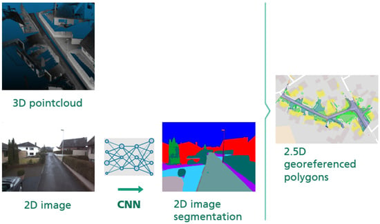
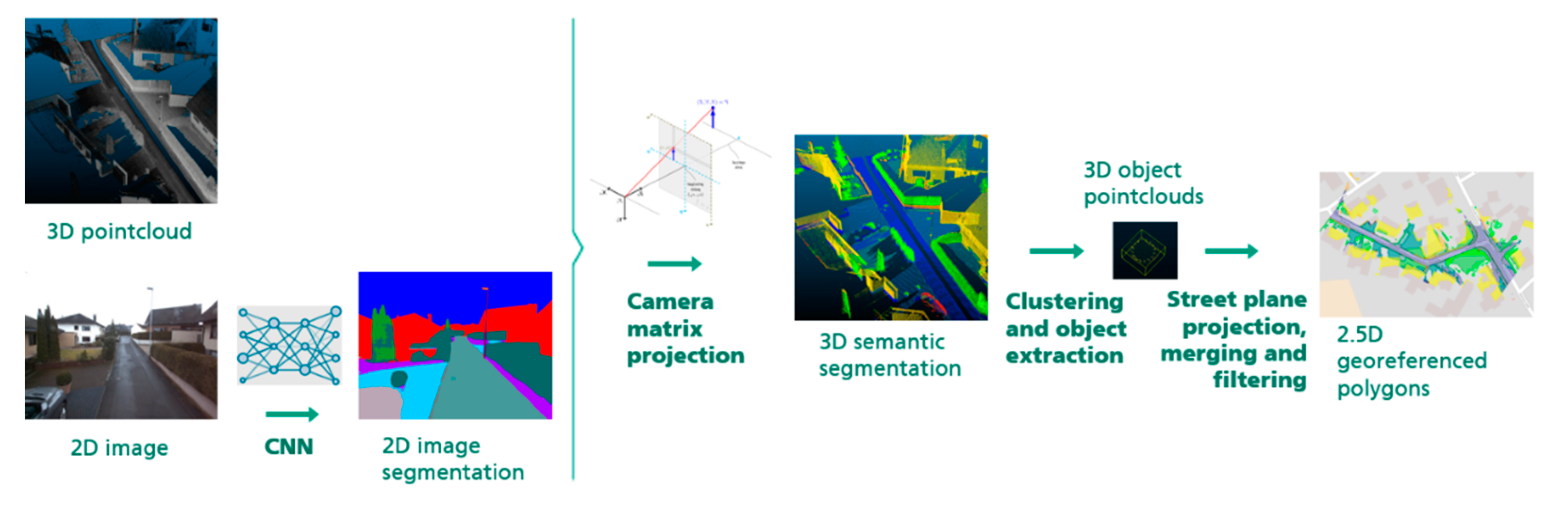
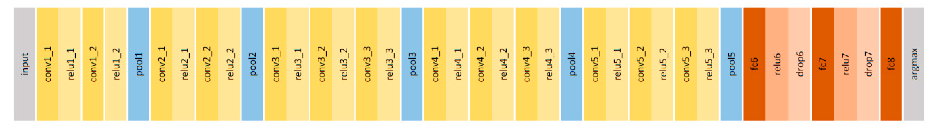
We present an approach specifically tailored to the application of digital planning for expanding a broadband network, utilizing mobile mapping data from both LiDAR (Light Detection and Ranging) and camera sensors. A key element of our approach is the use of supervised learning to train a convolutional neural network (CNN) that is able to distinguish surfaces and objects relevant to civil engineering (e.g., different types of pavement) in images captured by a mobile mapping system. We use this information to segment a dense point cloud, from which we extract localized objects and represent them as pairs of shape and height, yielding a 2.5D map of the recorded area with detailed surface texture information. The purpose of the resulting data stream is to inform a routing algorithm tasked with finding a reliable (i.e., not disrupted by objects hindering construction, such as rails) and cost-efficient (i.e., through surfaces that can be easily restored) route for construction work.

Deep learning techniques based on CNNs are the current state-of-the-art in computer vision, [8,9,10]. For object detection, classification, or segmentation in 3D data, only recently approaches based on deep learning have gained traction due the lower resolution compared to images and sparseness of the point cloud. Approaches can be categorized into volumetric (e.g., VoxNet [11], which transform the input point cloud into structured voxel data), point-wise (e.g., PointNet [12], which use points as input without a previous transformation), and multi-view-based (e.g., VoteNet. [13], where 3D point clouds are transferred into 2D images for classification or segmentation). Most recently, integrations of point-wise and volumetric methods have shown promise [14]. A comprehensive survey of methods for 3D classification can be found for example in the work of Reference [15].

Our approach can be placed within multi-view-based research, where most recently advanced ways of combining RGB and depth views of the point cloud have emerged, for example, with ImVoteNet [16]. However, our goal differs from most applications in the field, which work on classification of indoors scenes or autonomous driving applications; we focus on distinguishing urban surface textures, such as concrete, asphalt, pavement, or gravel, for which color information is an essential feature, while depth is negligible. Instead of working with depth or intensity 2D maps, we extract object information from RGB images only, which have been recorded synchronously with the point cloud and offer multiple perspectives of the objects and surfaces visible in the 3D data. A similar approach is described by Reference [17], who classified images with a CNN trained on the CityScapes dataset [18], mapped segmentation results to 3D points using camera parameters, and refined the result with features extracted from the point clouds. However, their pipeline stops at the classified point cloud, while our procedure also includes the extraction of object instances and their shapes for the creation of a digital map. Since—to our knowledge—there is no dataset publicly available at the current time that provides annotations of fine-grained classes of urban surface textures, a custom dataset of 90,000 segmented RGB images was created in the process of building our system, as well as an extensive reference map in two different locations in Germany.

In general, the focus of our paper is not on novel methods for individual steps of the pipeline (e.g., image or point cloud segmentation) but on the practical application of scene classification and reaching high accuracy and robustness in feasible processing time in practice; so far, little research has been conducted in this direction [19].

2. Materials and Methods

2.1. Mobile Mapping System and Data

Mobile mapping is the process of collecting data by means of a mobile caring platform (e.g., a car) equipped with different sensors [20]. The main sensor of such a system is the positioning and orientation sensor (POS), which represents a combination of an inertial measurement unit (IMU), a global navigation satellite system (GNSS), and an odometer (OD). Data streams from the POS, IMU, GNSS, and OD are fused to a trajectory using a Kalman filter, which calculates a continuous forward solution in real time. The calculated trajectory represents the route driven by the measurement vehicle including the corresponding spatial orientations in a global reference frame (referenced in time and space: x, y, z, alpha, beta, gamma, t). In a first step, this information refers to the origin of the POS. All other sensors are secondary sensors, which are synchronized with the POS by time or distance. These sensors can be video cameras, single frame cameras, LiDAR, or georadar systems. Once the position and orientation of all sensors in relation to the origin of the POS is known (usually determined by the extrinsic calibration of the entire system), all data can be brought into spatial relation to the common global frame. The result of a measurement run are georeferenced images and 3D points.

The measurement vehicle used for the project presented here is equipped with a LiDAR (the Fraunhofer Clearance Profile Scanner (CPS) with a measurement frequency of 2 MHz and a scanning frequency of 200 Hz), four cameras with a single resolution of 5 megapixel and a POS (Applanix LV420). The LiDAR data is generated and time-stamped in a free-running mode, whereas images are recorded in a way-triggered mode. The system synchronously captures four images every 5 m (aligned to the front, back, and sides). Examples of captured image and 3D points (point cloud) are shown in Figure 1 and Figure 2.

2.2. Processing Pipeline

Figure 3 contains a visualization of the full data processing pipeline. The software comprises two main stages and processes large chunks of mobile mapping data by splitting point clouds and images into smaller overlapping units of 20 m.

During the first stage, images receive a pixel-wise classification, resulting in a 2D semantic segmentation of all perspectives recorded by the mobile mapping vehicle. The segmentation is then transferred into the point cloud by projecting pixels onto points using the extrinsic calibration of scanner and respective camera. Many points have been recorded from multiple camera perspectives, so there are different options to use the label information to determine the final class of a point. We experimented with two strategies: (a) classify every point with the label information received from the camera position closest to the point; and (b) apply a voting scheme and classify every point with the majority class, if it received more than one label. The pixel-wise image classification is derived with a CNN using the well-established VGG16 encoder in an FCN 8 architecture [9] (Figure 4).

As most publicly available data sets for image segmentation focus on street objects and categories, such as sidewalk versus street, rather than details of the surface texture, a large dataset tailored specifically to the application was created from scratch to train the network. To make the system robust enough to deal with mobile mapping data from all over Germany, from different camera sensors and at different seasons of the year, a large and diverse set of data was recorded in advance. The collection was organized in three campaigns (from September until December 2017, in March 2018 and in August 2018) with two different mobile mapping vehicles in more than 20 locations. This resulted in a data collection of 1.3 million images, from which 90,000 images where handpicked—specifically looking for recordings of surface textures or objects that appeared rarely, such as concrete and rail tracks, or seasonal variations (Figure 5)—and annotated manually with a segmentation mask (for an example, see Figure 6).

Main classes, on which we focus in this paper, were surface textures (asphalt, concrete, gravel, grass, small pavement, and large pavement) and objects disrupting the road surface (rail tracks and curbstone). Additionally, helper classes, such as vehicles, building, people, road inventory, and more, were annotated (however, we do not report results on these classes currently, as the routing algorithm makes no use of them at the current time). We list target object classes and their appearance rate in the final training in

Table 1. Object classes ranked by relative pixel frequency in the manually produced segmentation masks for the training data set.

Object Class	Asphalt	Grass	Curbstone	Small Paving	Hole Cover	Gravel	Large Paving	Rail Tracks	Concrete
Appearance Rate	93%	80%	78%	59%	44%	13%	6%	4%	4%

.

The CNN was trained using the Caffe framework [5], which is especially suited for deployment in a large distributed application (the final pipeline runs in the cloud) and very robust. As the point cloud processing rather than the image processing is the bottleneck of our pipeline, speed was a lesser consideration in choosing the deep learning framework. We applied data augmentation especially adapted to the types of variations observed in the images produced by the two different mobile mapping camera systems. These were mainly strong shifts in color due to a dynamic white-balance adaptation thrown off by large colored areas in an image (such as the side of a bus or painted facades) and shifts in brightness due to sections of images frequently being over- and underexposed. This can be attributed to a slow exposure adaptation in settings with strong contrast, e.g., with bright sunlight. The final CNN was trained using the Adam optimizer [21] with Caffe default parameters. The best model was found after training for 7 epochs on the whole training dataset on a single Nvidia GTX 1080 over the course of three weeks.

The segmented point cloud is processed during the second stage (Figure 7): Using the object class information derived from the image projection, a plane is fitted using the subset of points that received a surface label in the voting scheme, using the RANSAC algorithm [22]. We then apply this information to label the point cloud a second time, prohibiting points from receiving surface labels that are not in close range of the assumed street plane and banning helper object labels from the street plane area.

This step is necessary to deal with the problem of the lower resolution of the point cloud and a useful heuristic to mitigate the effects of inaccurate extrinsic calibrations of sensors. Often, objects that are obscured by another object from a given camera perspective receive labels from the foreground object because the resolution of the object is lower in the point cloud than in the image and points “travel through”. The same effect can occur if objects are only partially present in the point cloud due to shading by other objects or objects that are see-through for the scanner but not for the camera (e.g., car windows). In addition to the street plane filter, we also use a depth filter, which restricts clusters of labels to a mutual depth plane, which helps with see-through objects, such as railings. We then apply object extraction by means of euclidean clustering on the label-filtered point cloud. The extracted point clusters are sorted by label and their points projected onto the street plane, from which a concave hull for each object instance or area is subsequently computed [23], resulting in a georeferenced polygon. The final step cleans and filters the resulting polygons based on class-specific parameters; finally, the pipeline merges polygons of the same class for adjacent point clouds to create a full and consistent map of the recorded area.

The inference time of the full pipeline depends on the available hardware, i.e., number of GPUs, CPUs and available memory. On a Workstation equipped with an Intel i9 9920X (12c/24t) CPU and 64GB Ram, Samsung 970 EVO SSD, and 2 Nvidia RTX2080 GPUs, the system was able to process 3.1 km of mobile mapping data per hour (mean over 7 data sets). However, the standard deviation of these measurements was quite high, at 0.86. While the first stage of the pipeline scales linearly with the number of images to classify, the processing time for the second stage depends on the point cloud density and the complexity of the scene (number of different classes, number of individual clusters).

3. Results

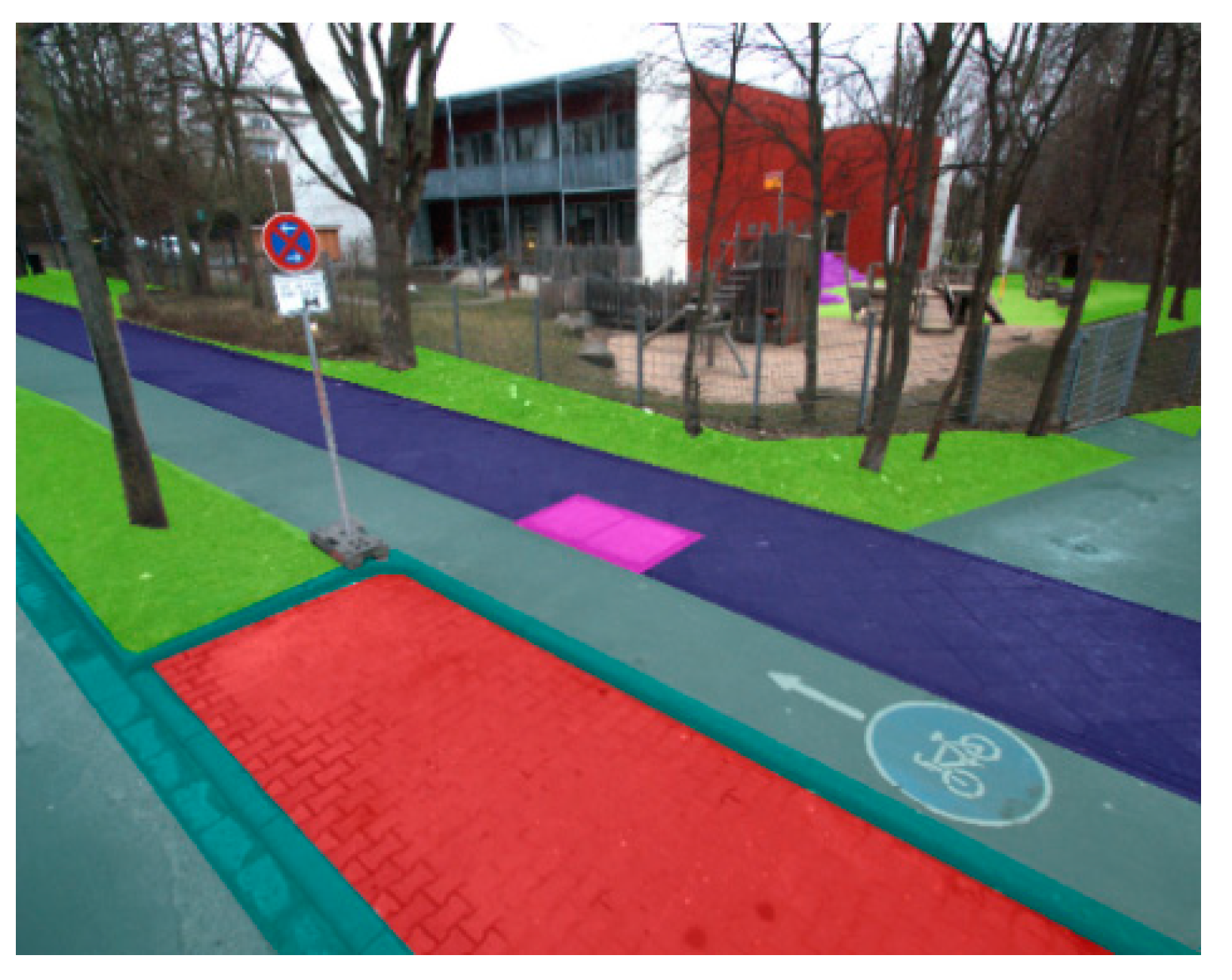
In the route planning process based on the stream of data output by our system, detected objects serve different information needs. Broadly, two types of objects are of interest for this application: surface textures and objects disrupting a continuous surface.

(a)

Surfaces, i.e., areas of ground covered with a specific material (e.g., asphalt or grass; see above). Knowing the exact extent of a surface is important in order to be able to calculate the cost of implementing a planned route though several areas and minimize this cost during the routing process (building through grass is cheaper than opening up pavement). We want to reflect this in our evaluation strategy and compute measures based on area overlap.

(b)

Disrupting objects, i.e., objects placed on or inside a surface, which may disrupt a potential broadband route, such as curbstones or rail tracks. The exact area size of these objects is less relevant for the application, since the route planning establishes buffer zones around disrupting objects; however, since undetected “holes” in continuous objects can significantly alter planned routes, high recall is important in the detection of these objects.

3.1. Reference Data Set

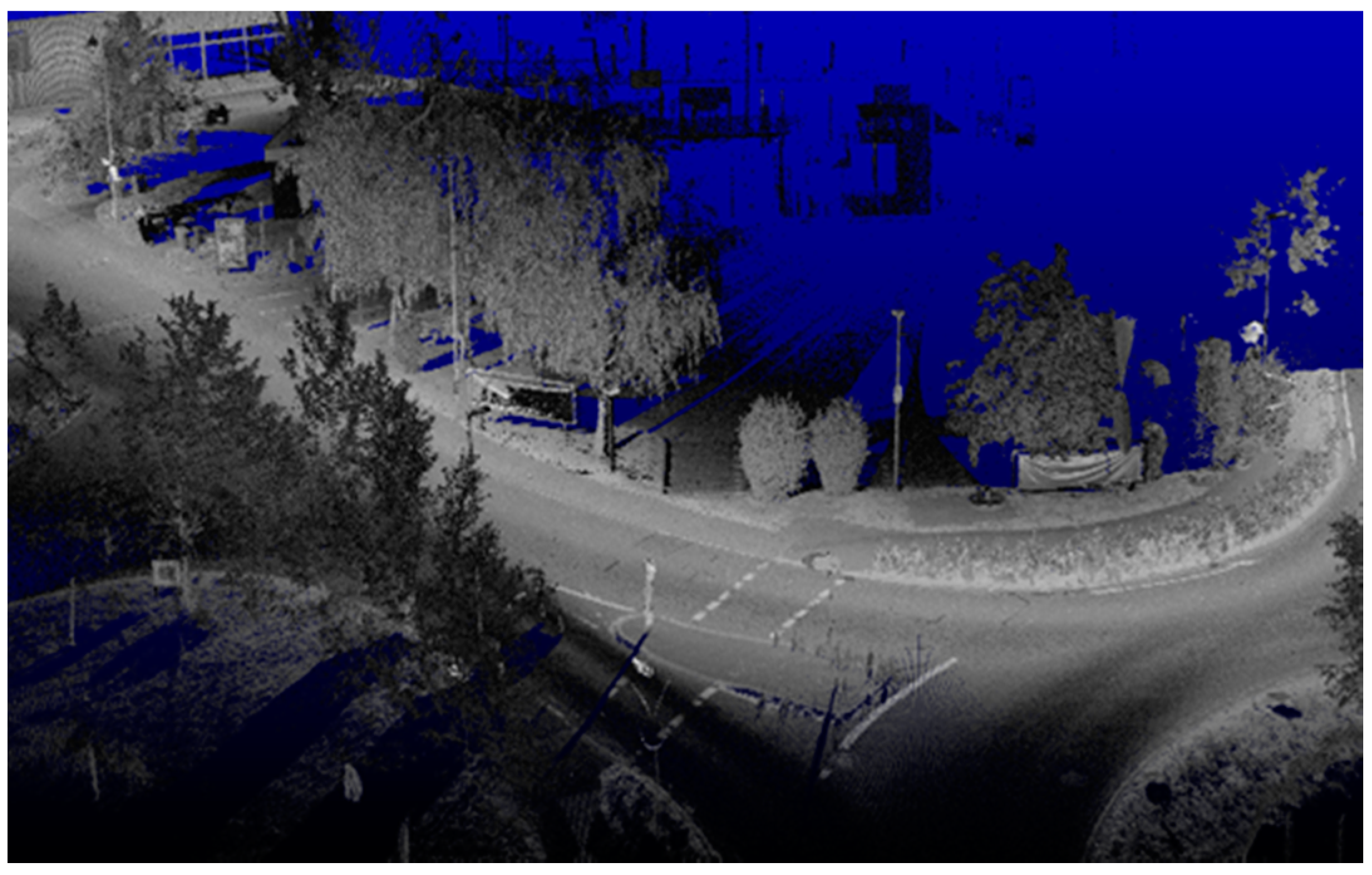
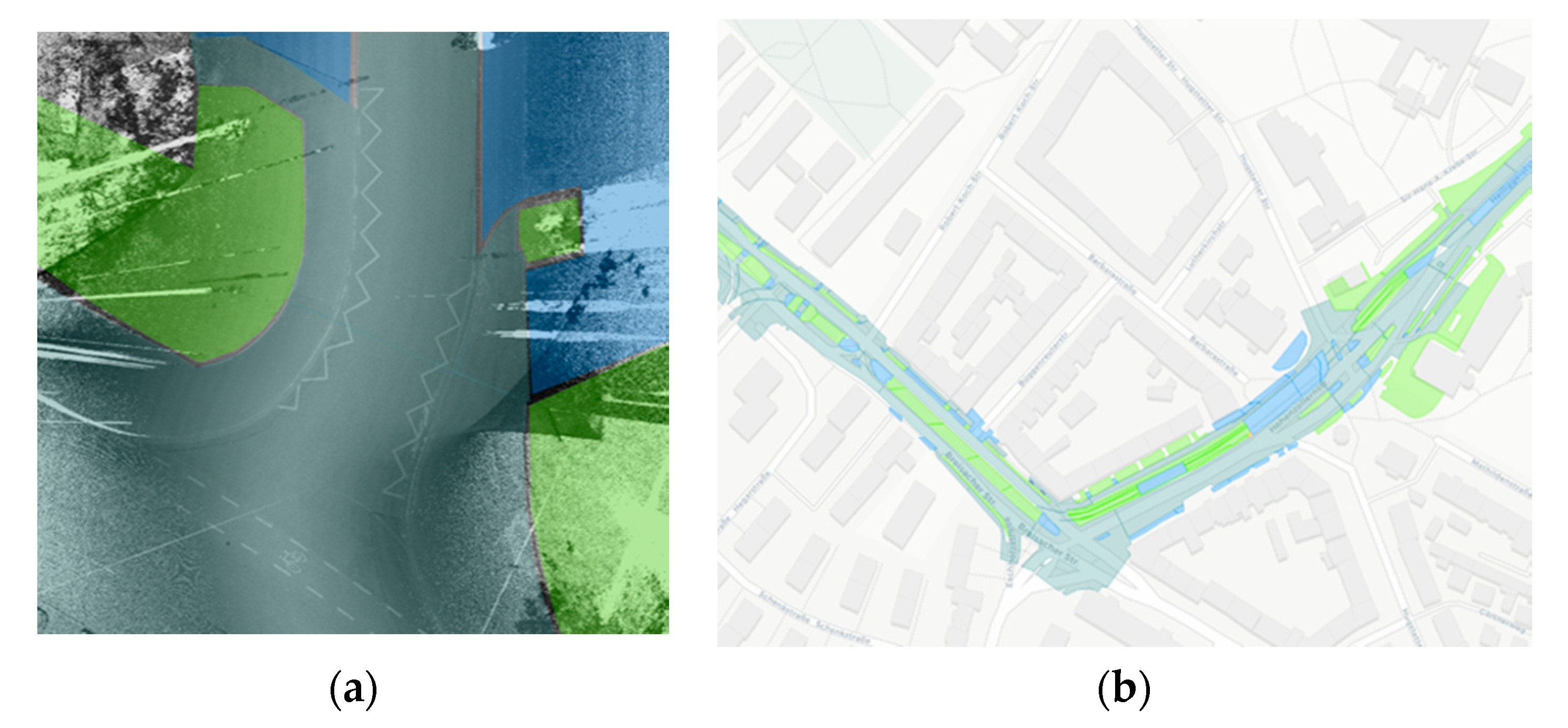
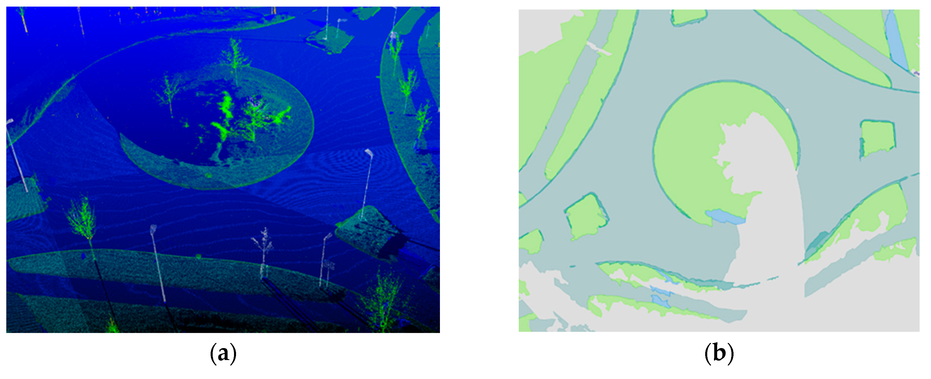
To guarantee that our system performs reliably in a real-world application with a broad range of different scenes, weather, and lighting settings all over Germany, we manually created an extensive reference map, covering all target objects and using diverse input data from various seasons and locations. We selected two areas for evaluation, for which data was recorded exclusively for evaluation and chronologically and geographically completely separate from the recording of the CNN training data, namely an inner-city area from Freiburg, Baden-Württemberg (Germany), and a mix of suburban and rural area from Bornheim, Nordrhein-Westfalen (Germany). Data from Bornheim was recorded in July 2018. For the Freiburg area, two recordings were available, from March 2018 and July 2018. We asked annotators to draw reference polygons of the shapes of surfaces and objects with the help of aerial images. Especially for narrow objects, such as curbstones and rail tracks, aerial images turned out to be far too low in resolution, as well as inaccurate in the exact localization of the objects. To solve this problem, we used birds-eye views of the point cloud, visualizing intensity values at different resolutions to help annotators identify reference shapes correctly, in combination with corresponding terrestrial images from the mobile mapping cameras, for identifying the surface texture correctly (see Figure 8). In total, five annotators worked on the ground truth, polygons for all objects were double-checked, and more than 150,000 square meters of highly detailed ground truth created, corresponding to a route of 8 kilometers driven by the mobile mapping vehicle. The data set covers the six surface texture classes (concrete, asphalt, large paving, small paving, grass, and gravel) and two disrupting object classes (rail tracks and curbstone).

3.2. Evaluation

As we work towards a real-world application, we focus on a detailed inspection of the final pipeline output, i.e. the quality and accuracy of 2D polygons, instead of intermediary results, such as the segmentation of images and point clouds. Still, we use notions about the output quality similar to measuring the performance of classifiers: we count True and False Positives, as well as False Negatives, and compute evaluation measures based on these numbers.

Table 2. Counts for area-based evaluation.

True Positives (TP)	Intersection area of output polygons of class A with ground truth polygons of class A
False Positives (FP)	Intersection area of output polygons of class A with ground truth polygons of class B, C, … (all classes ≠ A)
False Negatives (FN)	Intersection area of ground truth polygons of class A with output polygons of class B, C, … (all classes ≠ A)

shows the definition of these terms in the context of our task, Figure 9 a visualization. Based on these counts, we compute Precision, Recall, and F1-score.

Table 3. Results for all surface classes on all three evaluations sets with size of ground truth data in m2 for each class. Note that the ground truth sizes for three classes (concrete, large paving, and gravel) is very small on the Freiburg set, and the numbers are therefore not reliable (indicated in grey font).

Object Class	Freiburg (03/18)				Freiburg (07/18)			Bornheim				Total
	m²	Pr	Rc	F1	Pr	Rc	F1	m²	Pr	Rc	F1	m²	Pr	Rc	F1
concrete	409	49%	78%	60%	62%	65%	64%	3972	97%	90%	93%	4381	92%	89%	90%
asphalt	75,852	97%	97%	97%	94%	97%	95%	13,965	90%	97%	93%	89,818	94%	97%	96%
large paving	480	53%	47%	50%	58%	83%	68%	2089	89%	78%	83%	2569	81%	75%	78%
small paving	11,573	88%	88%	88%	89%	81%	85%	5997	94%	95%	94%	17,570	91%	89%	90%
grass/dirt	60,646	93%	94%	94%	91%	97%	94%	10,536	87%	97%	92%	71,182	91%	96%	93%
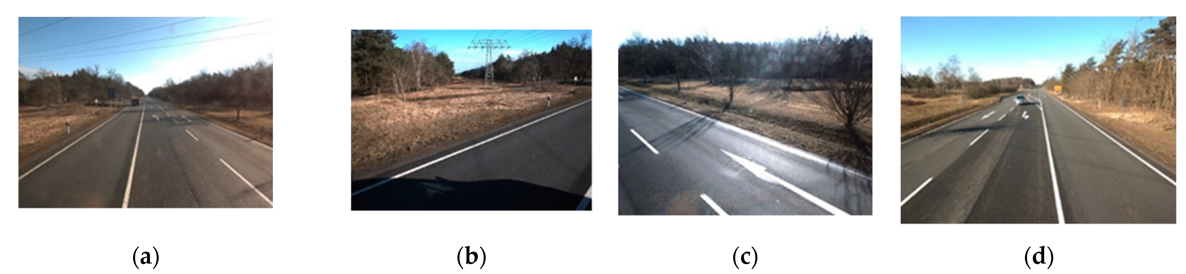
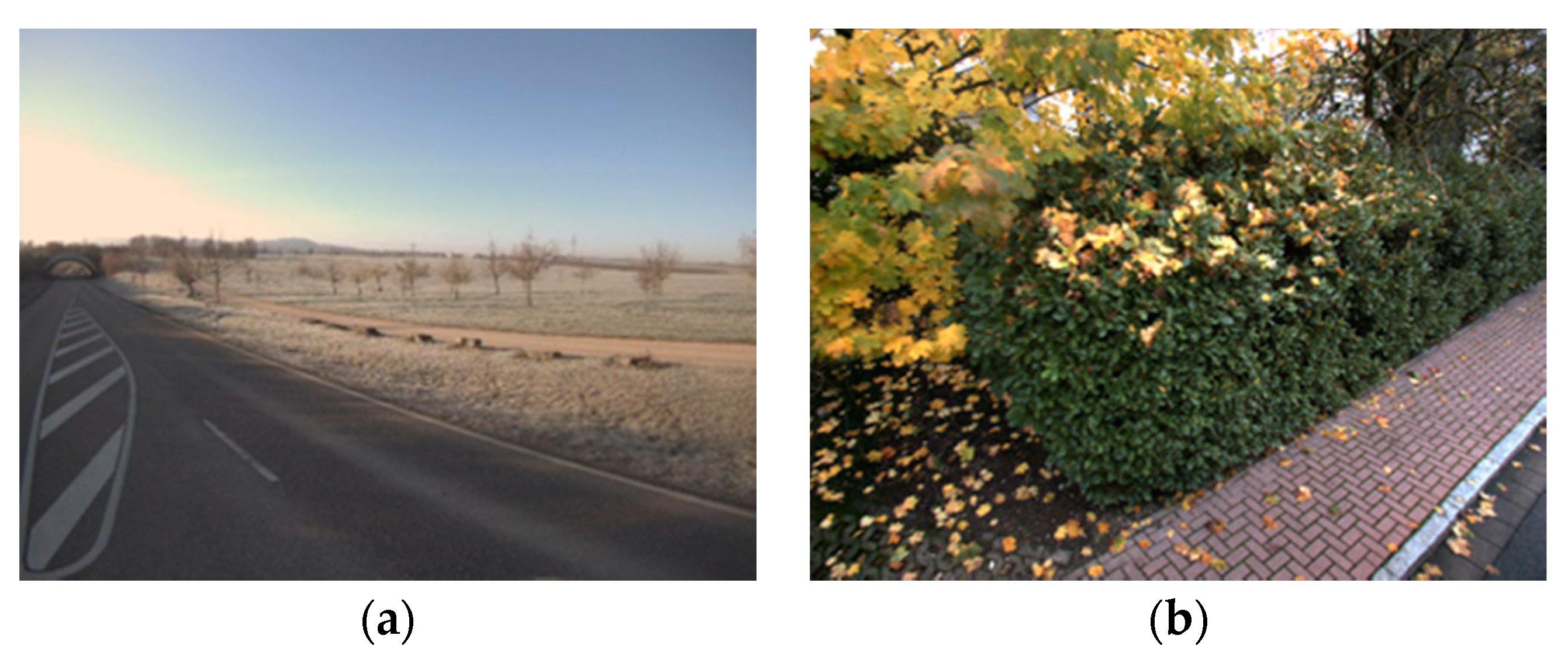
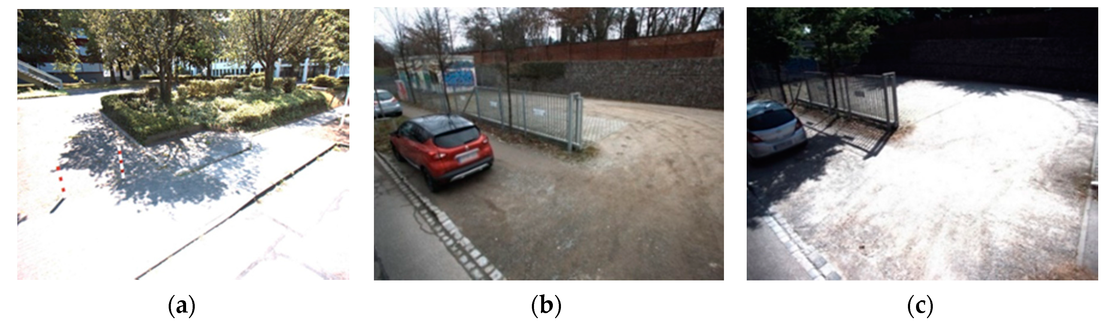
gravel	1820	65%	55%	60%	60%	30%	40%	17,585	98%	85%	91%	19,405	96%	82%	88%

shows the evaluation results for the six individual surface classes on all data sets separately and averaged. Results show that the system can distinguish even similar looking surfaces, such as concrete and asphalt, with high reliability (between 75% and 95%) when averaged over location and season. Note that we did not filter the evaluation data with regard to image quality, so the set contains images both with over- and underexposed regions. Especially, the data recorded in summer contains a significant number of images, in which critical parts are over- and underexposed.

We chose to keep this data in the evaluation set regardless, to gain a realistic impression of the capabilities of a system faced with incomplete and impaired data. Figure 10 shows examples. Overall, results are lower for classes for which less data is available in the reference set (such as large paving), corresponding to lower frequency in the training set.

The main challenge for our system is to distinguish reliably surface textures that look similar; overexposed asphalt may closely resemble concrete and images of concrete, where no boundaries are visible, and can be easily mistaken for asphalt, even by the human eye. Strongly distressed asphalt often resembles gravel, and the difference between dirt and gravel is fluid. The same holds true for the division into small and large paving. Even though the CNN handles scaling quite well due to the fixed perspectives, there are paving patterns consisting of both large and small stones, leading to ambiguous cases. We therefore performed a paired evaluation of related surfaces (see

Table 4. Combined evaluation of related surface classes (mean over all data sets).

Object Class	Pr	Rc	F1
asphalt + concrete	95%	97%	96%
paving	92%	90%	91%
grass, dirt + gravel	95%	95%	95%

). Precision and Recall for all combinations were up to 90% and higher, supporting the hypothesis that the system mostly confuses visually similar textures. The paired evaluation of the surface classes makes sense in the context of the application, as well. The difference in cost between construction works through the respective surfaces is much smaller within those pairs than between pairs, meaning the error in cost calculation is smaller, when there is a confusion between members of a pair.

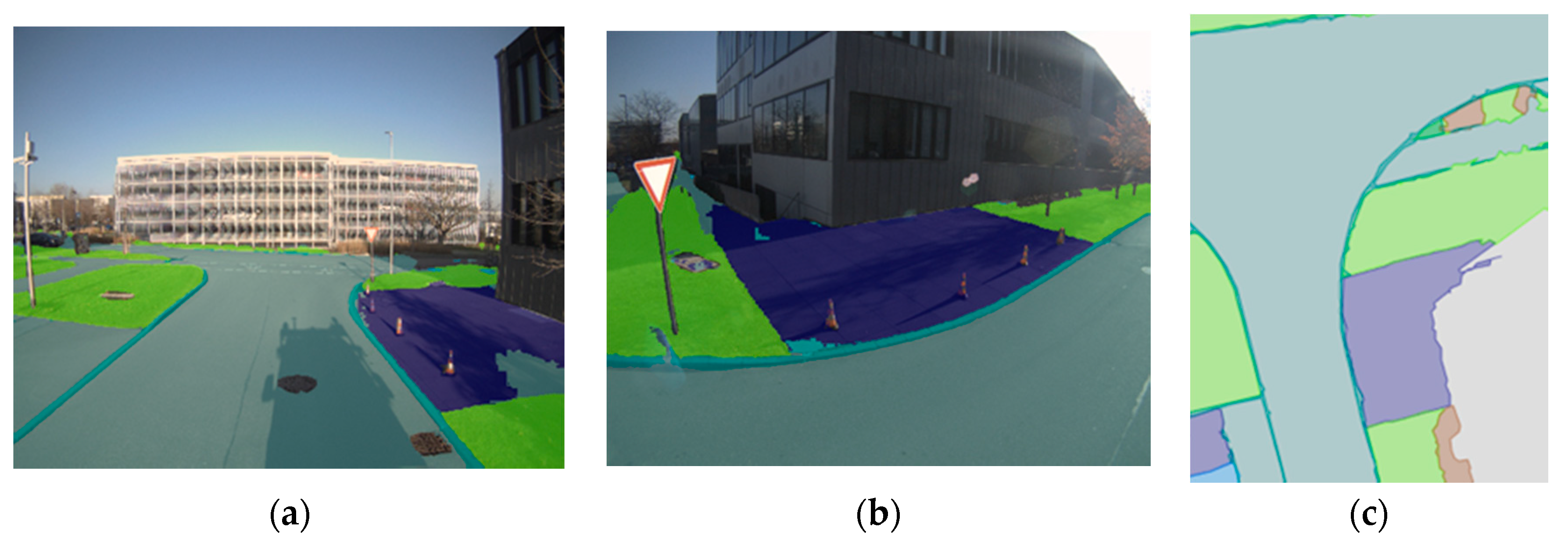
One aspect that makes the system robust in application is the availability of images taken from multiple perspectives. Surfaces that are further away or partially hidden may appear again in an image taken by a different camera. We experimented with two different settings for determining the label of a point based on information from different images: majority label (voting) and nearest label (nearest being the one received by the image taken from the camera position closest to the point in question).

Table 5. Majority point labeling scheme vs. nearest label scheme (mean F1-score).

Object Class	Majority Label	Nearest Label	Δ
concrete	89%	90%	+1%
asphalt	95%	96%	+1%
large paving	67%	78%	+11%
small paving	81%	90%	+9%
grass/dirt	88%	93%	+5%
gravel	73%	88%	+15%

contains the results. Especially for object classes that appear less frequently, such as paving and gravel, taking labeling information from the nearest camera improves final classification accuracy.

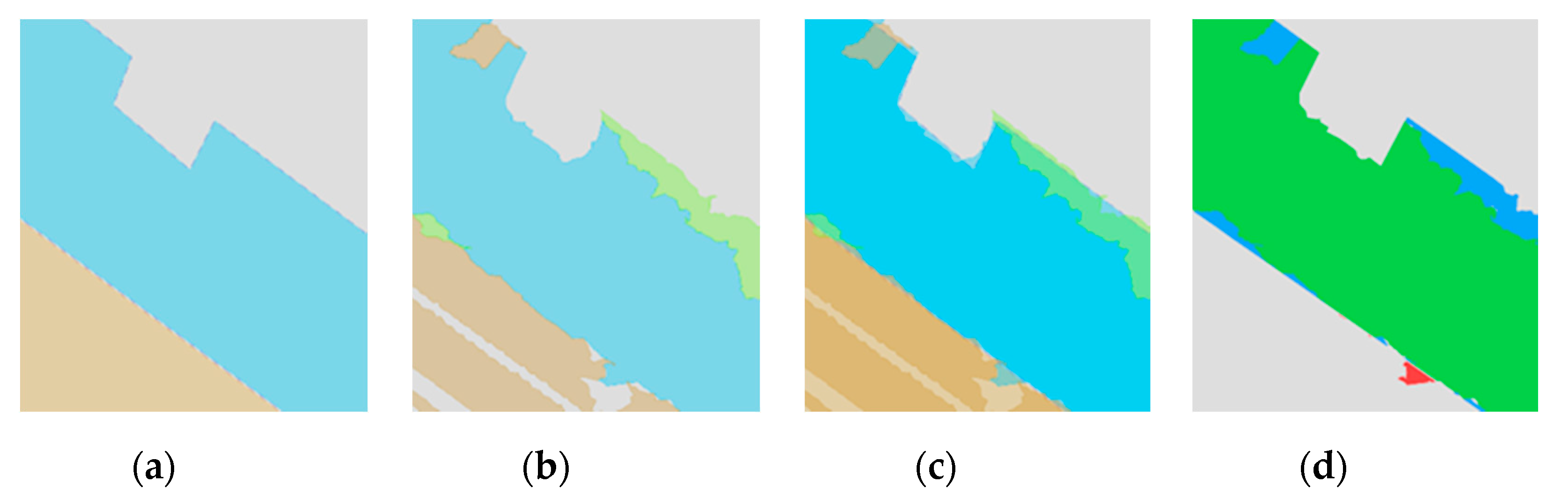
Figure 11 shows the surface segmentation for two images taken of the same surfaces but from different angles. Final output is a correct polygon for the whole area due to the higher weight given to labeling information received from images taken closer to the point in question. On the other hand, gaps in continuous objects are a regular occurrence caused by incomplete recordings of objects in 3D (Figure 12); this problem can be only fixed by changing the mode of data collection, e.g., by driving roads in both directions and adding additional LiDAR sensors at different angles.

Table 6. Evaluation results for disrupting object classes, rail tracks, and curbstone.

	Pr	Rc	F1
Rail Tracks	98%	83%	89%
Curbstone	94%	87%	90%

contains evaluation results for disrupting continuous objects, rail tracks, and curbstones. The results are conclusive; the percentage of False Positives is extremely low.

Note, that the ground truth annotation included parts of the objects that were obscured in 3D from the view point of the vehicle as discussed above, e.g., by parking or overtaking vehicles (again, we assume it is relevant to the application to assume input data may be incomplete regularly). Large continuous sections, where the object was obscured, e.g., at tram stations, which feature a high sidewalk on both sides of the track separating the rail tracks in the middle of the street from the driving lanes, were excluded from the annotation, though. The results should therefore closely reflect the performance of the system in application and the missing data accounts for the lower Recall compared to the high Precision. The larger presence of ambiguous objects can explain the lower precision for curbstones: in some cases, sidewalks feature intersecting stones, e.g., a paved line separating bike and pedestrian lane, which are visually indistinguishable from a low curbstone.

4. Conclusions

The paper at hand presents a study of how to apply deep learning techniques practically and successfully to a remote-sensing application with an extensive evaluation on real-world data. The focus of the work is on surface textures in urban scenes for the application of digital planning. Such a process is (to our knowledge) novel; frequently reported applications, such as land cover classification and autonomous driving, do not require the same level of detail in this area. Depending on the type of surface, our system achieves reliability levels of over 90%, and an implementation of the system is in productive use in the industry. However, due to this, we are not able to publish code and training data at the moment. In the future, we plan to expand the number of object classes make the approach robust for different levels of input data quality. The aim is to create a process chain that can be used universally-independent of the mobile mapping system and its sensor configuration.

References

1. Son, H.; Bosché, F.; Kim, C. As-built data acquisition and its use in production monitoring and automated layout of civil infrastructure: A survey. Adv. Eng. Inform. 2015, 29, 172–183. [Google Scholar] [CrossRef]
2. Walker, J.; Awange, J.L. Surveying for Civil and Mine Engineers. Theory, Workshops, and Practicals; Springer: Cham, Switzerland, 2018; ISBN 9783319531298. [Google Scholar]
3. El-Sheimy, N. An overview of mobile mapping systems. In Proceedings of the FIG Working Week 2005 and GSDI-8, Cairo, Egypt, 16–21 April 2005. [Google Scholar]
4. Puente, I.; González-Jorge, H.; Martínez-Sánchez, J.; Arias, P. Review of mobile mapping and surveying technologies. Measurement 2013, 46, 2127–2145. [Google Scholar] [CrossRef]
5. Jia, Y.; Shelhamer, E.; Donahue, J.; Karayev, S.; Long, J.; Girshick, R.; Guadarrama, S.; Darrell, T. Caffe: Convolutional architecture for fast feature embedding. arXiv 2014, arXiv:1408.5093. [Google Scholar]
6. Ma, L.; Li, Y.; Li, J.; Wang, C.; Wang, R.; Chapman, M. Mobile Laser scanned point-clouds for road object detection and extraction: A review. Remote Sens. 2018, 10, 1531. [Google Scholar] [CrossRef] [Green Version]
7. Che, E.; Jung, J.; Olsen, M.J. Object recognition, segmentation, and classification of mobile laser scanning point clouds: A state of the art review. Sensors 2019, 19, 810. [Google Scholar] [CrossRef] [PubMed] [Green Version]
8. Krizhevsky, A.; Sutskever, I.; Hinton, G.E. ImageNet classification with deep convolutional neural networks. In Advances in Neural Information Processing Systems, Tahoe City, CA, USA, 2012; Curran Associates Inc.: New York, NY, USA, 2012; pp. 1097–1105. [Google Scholar]
9. Long, J.; Shelhamer, E.; Darrell, T. Fully convolutional networks for semantic segmentation. In Proceedings of the 2015 IEEE Conference on Computer Vision and Pattern Recognition (CVPR), Boston, MA, USA, 7–12 June 2015; IEEE: Piscataway, NJ, USA, 2015; pp. 3431–3440. ISBN 9781467369640. [Google Scholar]
10. Chen, L.-C.; Zhu, Y.; Papandreou, G.; Schroff, F.; Adam, H. Encoder-decoder with atrous separable convolution for semantic image segmentation. arXiv 2018, arXiv:1802.02611. [Google Scholar]
11. Maturana, D.; Scherer, S. VoxNet: A 3D convolutional neural network for real-time object recognition. In Proceedings of the 2015 IEEE/RSJ International Conference on Intelligent Robots and Systems (IROS), Hamburg, Germany, 28 September–2 October 2015; pp. 922–928. [Google Scholar]
12. Qi, C.R.; Su, H.; Mo, K.; Guibas, L.J. PointNet: Deep learning on point sets for 3D classification and segmentation. arXiv 2016, arXiv:1612.00593. [Google Scholar]
13. Ding, Z.; Han, X.; Niethammer, M. VoteNet: A deep learning label fusion method for multi-atlas segmentation. arXiv 2019, arXiv:1904.08963. [Google Scholar]
14. Shi, S.; Guo, C.; Jiang, L.; Wang, Z.; Shi, J.; Wang, X.; Li, H. PV-RCNN: Point-voxel feature set abstraction for 3D object detection. arXiv 2019, arXiv:1912.13192. [Google Scholar]
15. Guo, Y.; Wang, H.; Hu, Q.; Liu, H.; Liu, L.; Bennamoun, M. Deep learning for 3D point clouds: A survey. arXiv 2019, arXiv:1912.12033. [Google Scholar] [CrossRef]
16. Qi, C.R.; Chen, X.; Litany, O.; Guibas, L.J. ImVoteNet: Boosting 3D object detection in point clouds with image votes. arXiv 2020, arXiv:2001.10692. [Google Scholar]
17. Zhang, R.; Li, G.; Li, M.; Wang, L. Fusion of images and point clouds for the semantic segmentation of large-scale 3D scenes based on deep learning. ISPRS J. Photogramm. Remote Sens. 2018, 143, 85–96. [Google Scholar] [CrossRef]
18. Cordts, M.; Omran, M.; Ramos, S.; Rehfeld, T.; Enzweiler, M.; Benenson, R.; Franke, U.; Roth, S.; Schiele, B. The cityscapes dataset for semantic urban scene understanding. arXiv 2016, arXiv:2001.10692. [Google Scholar]
19. Ma, L.; Liu, Y.; Zhang, X.; Ye, Y.; Yin, G.; Johnson, B.A. Deep learning in remote sensing applications: A meta-analysis and review. ISPRS J. Photogramm. Remote Sens. 2019, 152, 166–177. [Google Scholar] [CrossRef]
20. Tao, C.V. (Ed.) Advances in Mobile Mapping Technology; Taylor & Francis: London, UK, 2007; ISBN 9780415427234. [Google Scholar]
21. Kingma, D.P.; Ba, J. Adam: A method for stochastic optimization. arXiv 2014, arXiv:1412.6980. [Google Scholar]
22. Fischler, M.A.; Bolles, R.C. Random sample consensus: A paradigm for model fitting with applications to image analysis and automated cartography. Commun. ACM 1981, 24, 381–395. [Google Scholar] [CrossRef]
23. Moreira, A.J.C.; Santos, M.Y. Concave hull: A k-nearest neighbours approach for the computation of the region occupied by a set of points. In GRAPP 2007, Proceedings of the Second International Conference on Computer Graphics Theory and Applications, Barcelona, Spain, 8–11 March 2007; Institute for Systems and Technologies of Information, Control and Communication: Barcelona, Spain, 2007; pp. 61–68. [Google Scholar]
Figure 1. Three-dimensional point cloud (intensity values depicted in grayscale).
Remotesensing 12 02530 g001
Figure 2. Perspectives of the four cameras mounted on the mobile mapping vehicle: images taken with (a) front, (b) left, (c) right, and (d) rear camera. As the vehicle moves forward, it captures the road surface from different angles.
Remotesensing 12 02530 g002
Figure 3. Full processing pipeline (from left to right): 2D RGB images are processed with a convolutional neural network (CNN), resulting in a pixel-wise segmentation map. Using the camera parameters, the 2D segmentation is mapped onto 3D points, which are clustered to extract 3D objects. These objects are projected onto the computed street plane to generate a map with object height information.
Remotesensing 12 02530 g003
Figure 4. VGG16 feature extractor.
Remotesensing 12 02530 g004
Figure 5. Seasonal variation of surface textures: (a) frost on a stretch of grass; (b) shedded leaves.
Remotesensing 12 02530 g005
Figure 6. Manual surface segmentation (green: grass, red: small paving, blue: large paving, grey: asphalt: magenta: manhole cover, cyan: curbstone).
Remotesensing 12 02530 g006
Figure 7. Detailed description of the second stage of the pipeline: After the point cloud has received the initial labels from the segmented images, we fit a plane using all points that received a surface label, the street plane (white points in the second image). The point cloud is then labeled a second time using the street plane as a filter criterion: Points on or slightly above (up to 50 cm) the street plane will only receive surface labels, not labels from background objects, such as trees or cars. This removes shadows of foreground objects caused by points “traveling through” the object due to the lower resolution of the point cloud compared to the images. We extract object point clouds from the filtered point cloud by finding clusters of points that received the same class labels with euclidean clustering. We flatten these object clusters by projection onto the street plane and compute the concave hull for each flattened object, resulting in the final object polygon.
Remotesensing 12 02530 g007
Figure 8. Details of reference map. Polygons for asphalt (grey), grass or dirt (green), and small pavement (light blue). (a) With overlay of point cloud from birds-eye view; (b) OSM at maximum zoom.
Remotesensing 12 02530 g008
Figure 9. Computation of true and false positive areas for pavement (light blue): (a) Reference; (b) output; (c) overlay; (d) true positive (TP) (green), false positive (FP) (red), and false negative (FN) (blue).
Remotesensing 12 02530 g009
Figure 10. (a) Paved surface, strongly overexposed. Variation of input data quality due to different lighting conditions. Images show the same gravel surface recorded in (b) spring and (c) summer. Visibility is not improved in the following and preceding images.
Remotesensing 12 02530 g010
Figure 11. Classification of the same paved surface on an image taken by the front and tight camera. (a) Segmentation on the image taken with the front camera contains a spot, where the paved surface is misclassified as asphalt (grey); (b) in the image taken with a full view of the surface, it is correctly classified as large paving (dark blue); (c) correct polygon output.
Remotesensing 12 02530 g011
Figure 12. Incomplete polygon map (a) due to shading by a hill in the point cloud (b). It is possible to close this data gap with additional sensors or a more redundant recording strategy.
Remotesensing 12 02530 g012