Pixel-Wise Classification of High-Resolution Ground-Based Urban Hyperspectral Images with Convolutional Neural Networks


1
Biden School of Public Policy and Administration, University of Delaware, Newark, DE 19716, USA
2
Department of Civil and Environmental Engineering, University of Delaware, Newark, DE 19716, USA
3
Department of Physics and Astronomy, University of Delaware, Newark, DE 19716, USA
4
Data Science Institute, University of Delaware, Newark, DE 19716, USA
5
Center for Urban Science and Progress, New York University, New York, NY 11201, USA
*
Author to whom correspondence should be addressed.
Remote Sens. 2020, 12(16), 2540; https://0-doi-org.brum.beds.ac.uk/10.3390/rs12162540
Submission received: 3 July 2020
/
Revised: 2 August 2020
/
Accepted: 4 August 2020
/
Published: 7 August 2020
(This article belongs to the Special Issue Feature Extraction and Data Classification in Hyperspectral Imaging)
Abstract
:Using ground-based, remote hyperspectral images from 0.4–1.0 micron in ∼850 spectral channels—acquired with the Urban Observatory facility in New York City—we evaluate the use of one-dimensional Convolutional Neural Networks (CNNs) for pixel-level classification and segmentation of built and natural materials in urban environments. We find that a multi-class model trained on hand-labeled pixels containing Sky, Clouds, Vegetation, Water, Building facades, Windows, Roads, Cars, and Metal structures yields an accuracy of 90–97% for three different scenes. We assess the transferability of this model by training on one scene and testing to another with significantly different illumination conditions and/or different content. This results in a significant (∼45%) decrease in the model precision and recall as does training on all scenes at once and testing on the individual scenes. These results suggest that while CNNs are powerful tools for pixel-level classification of very high-resolution spectral data of urban environments, retraining between scenes may be necessary. Furthermore, we test the dependence of the model on several instrument- and data-specific parameters including reduced spectral resolution (down to 15 spectral channels) and number of available training instances. The results are strongly class-dependent; however, we find that the classification of natural materials is particularly robust, especially the Vegetation class with a precision and recall >94% for all scenes and model transfers and >90% with only a single training instance.
1. Introduction
As of 2018, more than 55% of the world’s population live in urban areas with a projection of up to 68% living in cities by 2050 [1]. Although cities cover less than 5% of the US land surface [2] and 0.5% of global land cover [3], urban environments have considerable impacts including energy consumption, air pollution, expanding material and impervious surfaces, etc. [4]—on both the human population and the environment, an effect that will become even more profound in the future [5]. Therefore, there is a growing need to accurately assess the spatial distribution and condition of materials, features, and structures of cities and their changes over time at high spatial resolution. Information on the classification of materials in urban environments is used as an input to a wide range of both operational and urban science applications from local municipal decision making including urban development planning [6], to the impacts of cites on local and global climate models [7,8].
Due to increasing technical capabilities, including instrument design and analysis techniques, remote sensing has become an important methodology for the mapping of objects and materials in rapidly expanding urban environments over recent decades [9]. One of the earliest examples of object classification in urban environments via remote sensing was in 1976 using aircraft and LANDSAT-1 satellite data [10]. In this work Kettig and Landgrebe propose a machine-learning algorithm, ECHO (extraction and classification of homogeneous objects) that uses both contextual and spectral information to segment multispectral images into agriculture, forest, town, mining, and water classifications. Over the following decades, the dependence of urban and geospatial studies on airborne and space-based remote observation has dramatically increased. In 2008, with a combination of high-resolution three-band color-infrared aerial imagery and LiDAR data of an area that included Baltimore City, MD., Zhou and Troy [11] classified objects into five classes: buildings, pavement, bare soil, fine textured vegetation and coarse textured vegetation with overall classification accuracy of 92.3%, and overall coefficient of 0.899. In 2009 Schneider et al. [3] used remotely sensed satellite data from the Moderate Resolution Imaging Spectroradiometer (MODIS) with 500 m spatial resolution and 36 spectral bands in the range of to to map the global distribution of urban land use, and achieved an overall accuracy of 93% at the pixel level and an overall coefficient of 0.65. More recently, Albert et al. (2017) [12] used large-scale satellite RGB imagery from Google Maps’ static API of 10 European cities, classified by the open source Urban Atlas survey into 10 land use classes, to analyze patterns in land use in urban neighborhoods. Their results showed that some types of urban environments are easier to infer than others, especially for classes that tend to be visually similar like agricultural lands and airports.
Surfaces in urban environments are geometrically complex and comprised of a variety of diverse materials. For this reason, hyperspectral imaging has an advantage over broadband imaging techniques due to its ability to identify materials using their unique spectral signatures over a wide range of wavelengths. Although broadband and multispectral imaging sensors generally range from 3 to 12 spectral channels [13], modern hyperspectral imagery and imaging spectrometry can incorporate several hundred to thousands of spectral bands. This increase in spectral resolution allows for the identification of surfaces and materials in urban scenes through their chemical and physical properties as well as the detection of (and correction for) the components of the atmosphere along the line of sight [14,15,16]. Hyperspectral imaging (HSI) segmentation (or classification), where each pixel is assigned a specific class based on its spectral and spatial characteristics, is currently an active field of research in the HSI community [17,18,19,20]. Although HSIs offer greater spectral resolution than multispectral images, they introduce significant challenges to image segmentation. The classification of pixels based on their spectra becomes a non-trivial task due to a variety of factors including changes in illumination, surface orientation, shadows, and environmental and atmospheric conditions. These complications have resulted in machine-learning classification becoming a major focus in the HSI remote-sensing literature (e.g. [21,22,23,24]).
In the last two decades, numerous pixel-wise machine-learning HSI classification methods have been studied including support vector machines (SVM) [25], multinomial logistic regression [26,27], boosted decision trees (DTs) [28], and neural networks [29,30,31] with varying degrees of success depending on the case and application. More recently, convolutional neural networks (CNNs [32,33]) a subclass of neural networks that was inspired by the neurological visual system [34] and that generate associations between spectral features through a cascade of learned filter shapes, have gained wide use for HSI segmentation tasks [35,36,37]. The popularity of CNNs in the HSI community can be attributed to several factors, including that CNNs do not necessarily incorporate handcrafted features and that (by design) CNNs learn coherent associations between nearby spectral channels. Moreover, given sufficient training data, CNNs have shown significant potential to accurately recognize objects while achieving generalizability of the features used to describe the objects [38].
In this paper, we examine the use of one-dimensional CNN models to segment ground-based, side-facing HSI images of urban scenes at high spatial and spectral resolution, assessing model transferability across scenes as well as performance as a function of spectral resolution and the number of pixels used for training. The main objectives of this work are the following:
- identifying the wavelength scale of spectral features in urban scenes;
- testing the extent to which the addition of spatial information contributes to CNN model performance when segmenting these scenes;
- comparing the performance of CNN models trained and tested on each scene separately as well as a single CNN model trained on all scenes at once;
- assessing the transferability of the CNN models by training on one scene and testing on another;
- evaluating the performance of CNN models as the spectral resolution is reduced;
- evaluating the performance of a CNN model as the number of training instances is reduced.
Taken together, these tasks assess both the ability of our models to segment HSI data of dense urban scenes from a side-facing vantage point, as well as the difficulty of applying our models to data from different instruments and of different scenes.
This article is organized as follows: in Section 2 we present the high-resolution HSI data used for training and testing, as well as details of the model architectures, training, and assessment. In Section 3 we describe the results of model segmentation performance and accuracy as a function of scene, pixel classification, and training set size, with further diagnostic confusion matrices in Appendix A. We then discuss our findings in Section 4 and summarize our conclusions in Section 5. We also provide the results of segmentation using Tree-based and Support Vector Machine models in Appendix B to provide comparisons of CNN model performance with other popular pixel-based segmentation methods.
2. Materials and Methods
2.1. Hyperspectral Imaging Data from the Urban Observatory
The HSI data used to train and test the performance of segmentation models in this work was acquired with the ‘Urban Observatory’ (UO) facility in New York City (NYC). The UO is a multi-scale, multi-modal observational platform for the study of dynamical processes in cities [39,40,41]. In addition to broadband visible and infrared imaging capabilities, the UO has deployed both VNIR [42,43] and Long Wave Infrared (LWIR) [44] HSI cameras to continuously image large swaths of NYC with persistence and temporal granularity on the order of minutes.
To build our models, we use data from two separate UO-deployed VNIR instruments that were sited atop a tall ∼120 m (∼400 ft) building in Brooklyn with both North- and South-facing vantage points and aligned horizontally as seen in Figure 1. These instruments were both single slit scanning spectrographs with 1600 vertical pixels and a characteristic spectral resolution (FWHM) of 0.72 nm, though they have slightly different spectral ranges. The North-facing VNIR was sensitive from 400.46 nm to 1031.29 nm in 872 spectral channels while the South-facing VNIR was sensitive to 395.46 nm to 1008.06 nm in 848 spectral channels. These instruments acquired 3 urban scenes: two south-facing images covering Downtown and North Brooklyn (one at 2 pm and one at 6 pm on different days, henceforth referred to as Scene 1-a and Scene 1-b respectively) and one north-facing image (Scene 2) of northern Brooklyn and Manhattan. Given the different spectral ranges and horizontal fields of view (set by the range of the panning of the spectrograph), the shapes of the datacubes (# row pixels × # column pixels × # wavelength channels) are for Scenes 1-a and 1-b as depicted in Figure 1, and for Scene 2. Figure 1 also shows composite RGB images of the three scenes produced by mapping the 610 nm, 540 nm, and 475 nm channels to the red, green, and blue values respectively.
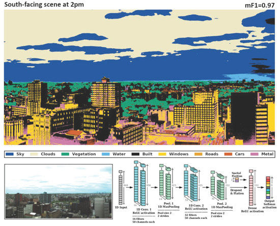
Given the high spectral resolution and sensitivity of the HSI instruments, each pixel in these hyperspectral images contains a wealth of information—from both subtle and dramatic variations in the shape of one pixel spectrum compared to another—about the type of material it covers. This encoding of material type is visualized in a false-color representation of Scene 1-a in Figure 2. Here the blue channel is mapped to ∼740 nm for which vegetation spectra have a strong peak (see Figure 1) while the red and green channels are mapped to wavelengths that highlight the difference in materials of built structures. The implication is that with only 3-bands, we can already see that high-resolution spectra have utility for segmenting an urban scene, suggesting that powerful supervised learning models trained with hand-labeled data have the potential for high-accuracy segmentation results.
For the purposes of training the models described below and evaluating their performance, ground truths were obtained via a subset of pixels from each UO HSI image that were manually classified into the following classes: Sky, Clouds, Vegetation, Water, Building facades, Windows, Roads, Cars, and Metal structures. Please note that in order to generate a balanced training set on which to train our machine-learning algorithms, we do not randomly select pixels from the scene to hand label. Doing so in this case would result in a sample heavily biased towards classes of materials that dominate the image—for example, sky and cloud pixels constitute ∼50% of pixels in Scenes 1-a and 1-b as shown in Figure 1. Therefore, 3200, 3555, and 4705 pixels in Scenes 1-a, 1-b, and 2 respectively were manually selected and labeled. Figure 3 shows the positions of the manually classified pixels superimposed over the images, together with a list of the number of pixels classified as each class of objects and materials. The figure also shows the mean (standardized) spectrum of each class of pixels in each scene. Due to lack of visibility from atmospheric conditions in Scene 1-b, no Water pixels were classified.
Sampling strategy for obtaining fair and sufficiently representative training examples is a widely discussed topic in the literature [45,46,47]. In addition to the sampling method described in this work, we attempted various approaches to selecting our training sets including: (a) using equal numbers of samples of Sky, Clouds, Vegetation, Building facades, and Windows (300 samples each), excluding the classes with 100 or less labeled examples, and testing on only those samples represented in the training set; and (b) using equal numbers of samples of Sky, Clouds, Vegetation, Building facades, and Windows (300 samples each) and including the classes with 100 or less total number of labeled examples. In both cases, the resulting performance of the models were within 1% of the scores of the models presented in this work, both overall and on a by-class basis.
2.2. Model Architecture
By design, Deep Convolutional Neural Networks incorporate a hierarchical feature identification and grouping architecture into the learning process that is well-suited to spectroscopic classification [35,36,37]. In particular, structure in the reflection spectra of built and natural materials at high resolution (spectral lines) and groupings thereof into lower resolution (spectral shapes and spectral illumination properties) are not only what differentiates the various classes phenomenologically, but they are also amenable to being learned as the 1-dimensional convolution kernels (filters) at various layers in the network. For example, a learned filter in the first layers of a network that corresponds to an absorption line may not be, by itself, discriminatory among the various classes; however groups of absorption lines—learned deeper in the network after further convolution and pooling layers—may be.
We perform our classification task with two CNN models (hereafter Model 1 and Model 2) that have identical architecture, but with different numbers and widths of their convolutional filters. The choice of filter parameters for the two models in the hidden layers is determined following the procedure described in Section 3.1 and explored further in Section 3.2. Their architecture is shown in Figure 4 and consists of a 1-dimensional input layer of 848 spectral channels, followed by two convolutional and max-pooling layers. Please note that the HSI datacubes provided in this work do not contain the true geographic positions of each pixel in the images, therefore the only spatial information that can assist in the classification tasks is that of the row and column coordinates of each pixel in the image. Hence, the output of the two convolutional and max-pooling layers is flattened and concatenated with 2 spatial components (fractional row and column coordinates), which then become the inputs to a fully connected layer (see Figure 4). Therefore, even though the initial input to the CNN is the 1D spectrum of each pixel, this full connectivity with the spatial coordinates towards the end of the network implies that the location of the pixel in the image is integrated with all wavelengths by the model. This fully connected layer is then followed by an output layer of 9 neurons representing the 9 possible manually classified material types. A ReLU (Rectified Linear Unit) [48] activation function was used in each convolutional and fully connected layer, and a SoftMax activation was applied to the output layer to estimate relative probabilities for each classification.
2.3. Model Training and Assessment
Prior to training our CNN models (including the tuning of the filter size hyperparameters), the spectra of our manually classified pixels in all three scenes were standardized using Gaussian normalization [49],
where is the raw spectrum of pixel i as a function of wavelength and and are mean and standard deviation (respectively) of the raw spectrum over all wavelengths. Thus, the standardized spectrum has mean 0 and standard deviation 1. In addition, in order to ensure that our models are transferable between scenes, the standardized spectra of pixels from the north-facing instrument were interpolated onto the same wavelength bins as those from the south-facing instrument. Please note that this is required by the architecture of our CNN-based models below.
The manually classified, standardized pixels were randomly split into 80% training and 20% testing sets in each UO HSI scene, and the split was done with stratification, where each set contains the same distribution of instances among the classes as the overall data set. We used multiple metrics to describe the performance of each model, and to account for the class imbalance problem we employed per class metrics and their weighted means over all classes. The per class metrics used in this work are the Precision (the ratio of instances correctly identified as in class that actually are in that class), Recall (the percentage of instances in a given class that were correctly recognized by the model as being in said class), and Measure. The Measure (or Score) represents a harmonic mean between Precision and Recall that tends to be closer to the smaller of the two, with a high value indicating that both Precision and Recall are high [50,51]. To quantify the performance of each CNN model as a whole rather than by class, the means of the per class metrics were calculated with a weighting set by the number of test instances in each class.
For training and loss minimization, we use the Adam optimizer [52] for each model with the loss specified by the sparse categorical cross-entropy. The number of epochs used for training was chosen as the elbow point of the loss evaluated on the testing set, and we verified that further training iterations only resulted in overfitting, with the loss on the training set continuing to decrease without a corresponding decrease in the testing set loss. Our procedure for each model is then summarized as follows: For a given scene, pixel spectra are extracted (as shown in Figure 1) and standardized, then fed individually through the model as shown in Figure 4 to obtain classifications. The performance of the model is then quantified using the hand-labeled pixels in Figure 3. With a single core on an Intel Xeon E7 4830 V4 2.00 GHz processor, training Model 2 (Figure 4) using 2560 training examples at full 848 channel spectral resolution each, with 640 validation examples for 200 epochs takes an average of 10 min. Once trained, the model takes an average of ∼0.4 microsecond to classify a given spectrum, resulting in roughly 20 min to predict the classifications of all 2,560,000 pixels () in our scenes.
3. Results
In the results described below, we trained our CNN models (shown in Figure 4) on the hand-labeled pixels from Figure 3 to address the six goals described in Section 1 that are designed to determine the models’ utility in segmenting and classifying pixels in urban hyperspectral imaging.
3.1. Identifying the Scale of Spectral Features in Urban Scenes
Much like CNN-based object identification tasks in 2-dimensional images, spectral CNN classification tasks in 1-dimension require a tuning of the filter sizes to match the pixel scale of distinguishing characteristics of the data. For example, if a spectrum of a given class has an absorption line that effectively distinguishes it from other classes and if that absorption line is of width 20 nm in a spectrum with 1 nm resolution (i.e., 20 pixels wide) then choosing convolutional filters in the first layer of width 5 pixels may be too small to effectively capture that feature. On the other hand, the learning of filters that are too large may be dominated by larger scale characteristics in the spectrum and not take optimal advantage of fine scale spectral structure. Thus, the performance of CNN models is dependent on choosing appropriate filters sizes in the convolutional layers.
Figure 5 shows the overall classification performance of our CNN architecture on Scene 1-a with filters of various kernel sizes in the convolutional layers while holding all other parameters constant. All metrics obtained from the test instances in Scene 1-a indicate that for the chosen CNN architecture, models with filters consisting of 50 spectral channels (∼35 nm wide) yield optimal performance with a mean score of 0.97 and testing accuracy of . Models with filter sizes smaller and larger than this had reduced performance. For example, a model with kernel size of 5 spectral channels (∼3.5 nm wide) resulted in a mean score of 0.89 and testing accuracy of , while a model incorporating filters with 200 channels (∼144 nm wide) resulted in a mean score of 0.91 and testing accuracy of . Taken together, these performance metrics indicate that pixel spectra in urban HSI data have features ∼30 nm wide that effectively discriminate among (built and natural) material types.
3.2. Comparing the Lowest and Highest Performing Models
The classification and segmentation results in this and the following sections are derived from two models with identical architectures, but different filter size hyperparameters: Model 1 has 32 filters in the first convolutional layer and 64 filters in the second, each with a width of 5 spectral channels (3.6 nm), while Model 2 has 16 filters in the first layer and 32 in the second, each with a width of 50 spectral channels (36 nm). These two cases are shown in Figure 4 and bracket the lowest and highest performing models in Figure 5. Model 1 and Model 2 were trained on each of the three scenes separately for a total of 6 trained models.
Figure 6 shows the results of applying each model on the image on which it was trained to predict the classes of all its pixels. We find that Model 2 performed better at classifying hand-labeled pixels in the testing set once trained on the hand-labeled training set for all three scenes. In particular, the mean score among classes for Scenes 1-a, 1-b, and 2 were 0.89, 0.86, and 0.82 (respectively) for Model 1 and 0.97, 0.92, and 0.90 for Model 2 demonstrating the improvement in segmentation results for convolutional features of width ∼35 nm compared to ∼3.5 nm. This is also visible qualitatively in the segmentation maps shown in the figure especially in the differentiation between the human-built materials by Model 2 in Scene 1-a and Scene 2 compared to that by Model 1. The following are some examples of this behavior: in Scene 1-a, Model 2 more accurately discerned Windows in the buildings in the lower left quadrant of the image than Model 1 which did not differentiate them from the building facade; in Scene 1-b, the buildings in the lower left corner have more of their windows identified as such by Model 2 than by Model 1; in Scene 2, Model 2 identified the road and cars in the lower left quadrant of the scene, as well as the rooftop of the building in the lower right corner, more accurately than Model 1.
The per class metrics for precision, recall, and score evaluated on the testing set are shown in Table 1 for each HSI image and for both models. The support column indicates the number of testing pixels in each class of materials and is used to calculate the weighted means for each class metric using the percentage of support pixels in a given class. The table shows that both models from all 3 images classified natural materials (i.e., Sky, Clouds, Vegetation, and Water pixels) with consistently high precision and recall, for each of these classes in all cases (Scene 1-b does not include Water pixels given their distance and the visibility at the time of the scan). For the remaining classes—which represent the human-built materials—Model 2 outperformed Model 1 for all classes when trained and tested on each scene indicating the dependence of classification on CNN model hyperparameters. These results are discussed further in Section 4.1.
3.3. Evaluating the Effect of Spatial Information
Recently, spatial features have been reported to improve the representation of hyperspectral data and increase classification accuracy [53,54]. In high-spatial-resolution images, objects and structures typically span multiple adjacent pixels. An object that is larger than a single pixel composed of the same material results in multiple adjacent pixels exhibiting similar spectral features. Therefore, the identification of materials in HSIs by classifiers can be improved by integrating the spectral features with the spatial locations of pixels. To this end, spatial features were included in the models tested in Section 3.1 and Section 3.2 by concatenating the fractional row and column coordinates with the flattened output of the last max-pooling layer as visualized in Figure 4. This concatenated layer then becomes input to a fully connected layer with a ReLU activation function, resulting in a spatial-spectral model that incorporates the location of pixels in the image at every wavelength. Here we evaluate the extent of the contribution of the added spatial information to the performance of the CNN model as opposed to that of the pure spectral information of pixel classes.
To do so we retrain Model 2 without adding the spatial information to the flattened output, and compare the model’s performance to that of the model with the spatial information included as shown in Section 3.2. As before, the models were trained using 80% of the manually classified pixels from each scene chosen randomly with stratification, and the trained models were then used to predict the classifications of all pixels in each of the three images. The performance of the models were assessed using the remaining 20% manually classified pixels in each scene. The resulting metrics of both model variants (i.e., with and without spatial features) are shown in Table 2 with the resulting pixel-wise image segmentation in Figure 7.
It is difficult to discern qualitatively which of the two model variants (with or without spatial information) in Figure 7 performed better at segmenting a given scene; however, some examples of the differences include the increased accuracy in classifying windows in the buildings in the lower left corner of Scene 1-a, as well as the misclassified cloud pixels on the horizon of Scene 1-b. Nevertheless, Table 2 shows that excluding spatial features resulted in a reduction in the performance of a given model. This reduction in performance is largely attributed to the decrease in classification performance of human-built materials while performance on natural materials remained near 100%. These results are further discussed in Section 4.2.
Several authors have shown that using 2D-CNN [22,35,55] and 3D-CNN [56,57] models that incorporate spatial-spectral context information by including the spectra of nearby pixels provides enhanced performance over 1D-CNN models. While one of the aims of this work is to isolate the effects of spectral classifications with a simpler 1D-CNN model, we also tested a model that included some spatial context information by concatenating the luminosities of all pixels in an square surrounding each pixel into the spatial features input into the final dense layer in Figure 4. Retraining Model 2 with this additional spatial context results in performance within 1% (in overall score and on a by-class basis) of the model with the relative pixel locations alone. Further model enhancements that include spatial-spectral features (i.e., the full spectra of surrounding pixels as opposed to only their luminosities) as input to the full network in Figure 4 for the classification of the UO’s side-facing, urban hyperspectral images will be the subject of future work.
3.4. Single Model Trained on All Scenes
So far we have explored training and testing individual CNN models on each image independently, with the results indicating that the ability of a CNN to properly generalize the learning of features from the training examples is influenced by the existence of shadows, and varying illumination and atmospheric conditions. Scene 1-a has optimal illumination conditions and therefore produces uniform spectra, which allow CNNs to predict the classification of pixels with greater precision and recall than Scenes 1-b and 2 which contain a significant amount of shadow and haze. Therefore, the question arises as to whether there is a benefit in training a single model using all available training instances from the three HSI scenes as opposed to training three separate models.
To test this, we use Model 2 (Figure 4) with 80% of hand-labeled pixels from all three scenes simultaneously (selected randomly and with stratification) to train the new model. We then test its classification performance using the remaining 20% of hand-labeled pixels as the testing sets. The resulting pixel-wise image segmentation maps using this model compared to that of using three separate models trained and tested on each image separately are shown in Figure 8, with their performance metrics on the testing sets quantified in Table 3.
In general, the self-trained models that are trained on each image separately perform better than this “all”-trained model trained using all three images simultaneously. In Figure 8 some examples of the self-trained models outperforming the all-trained model are seen in the middle of Scene 1-a where the windows are more accurately identified than in the all-trained model. In Scene 1-b the sky on the horizon at the left of the image is classified as buildings by the all-trained model, and in Scene 2 much of the buildings close to the horizon are misclassified as Water. Nevertheless, Table 3 shows that overall, self-trained models exhibited classification performance no more than 2% greater in terms of the mean metrics than that of the all-trained model. On a by-class basis, both model variants identified the natural materials (i.e., Sky, Clouds, Vegetation and Water) with equal and almost perfect precision and recall in every image. The marginal difference in the overall performance is entirely driven by the difference in classification of the human-made materials. This result indicates that natural materials can be generalized by training on all available scenes to their distinct spectral features and remain detectable regardless of given scene. Human-built material classes on the other hand, have spectral features that are highly dependent on illumination conditions, therefore generalizing these features by including training examples under different illumination conditions to the same model results in reduced classification accuracy when testing on each image individually.
3.5. Transferability of the Model
Testing the transferability of a CNN model requires the training of the model on a manually classified set of spectra from a hyperspectral image and evaluating the model’s classification performance on manually classified pixels from a different hyperspectral image. This test addresses the feasibility of training a single model and using that to automate the process of segmenting future HSI data of urban environments without the need to retrain the model on every image. As we described above and show in Figure 1, Scene 1-a has illumination conditions that produce uniform spectra among pixels of the same classification which leads to enhanced performance by the simple 1-dimensional CNN model (see Section 3.2). Given that our models perform best on Scene 1-a, this section assesses model transferability using models trained on Scene 1-a applied to Scene 1-b and 2. Note, the training procedure remains as described in Section 2, using the same hyperparameters for Models 1 and 2 in Section 3.2 and visualized in Figure 4. Although we showed in Section 3.3 that including spatial information when training the model produces overall higher classification accuracies, the spatial information was excluded when training the model for the purpose of transferring. As seen in Figure 3, some of the labeled instances are spatially dense with locations that are highly dependent on the given scene. Training a model using the spatial distribution of materials from Scene 1-a may produce unwanted effects when transferring to Scene 2 especially for some of the human-built materials like Roads, Cars, and Metal Structures. Therefore, the spatial information was excluded from training the models in this section.
The resulting pixel-wise image segmentation from both models trained on Scene 1-a and applied to Scenes 1-b and 2 are shown in Figure 9 and the per class and overall metrics evaluated on the testing sets from each image are summarized in Table 4. Please note that the entire set of labeled pixels described in Figure 3 for Scenes 1-b and 2 were used for testing.
Comparing the results of the transfer of both models in Figure 9 with those from training on each image individually in Figure 6, it is evident that transferring the models that were trained on Scene 1-a to Scenes 1-b and 2 caused a significant reduction in performance relative to models trained on each image independently. Qualitatively, the results of transferring both Model 1 and 2 to Scene 1-b resulted in the misclassification of almost all pixels above the horizon, as well as significant confusion in the human-built materials that are in shadows. These misclassifications are even more prominent when transferred to Scene 2 where the entire image is dominated by either Building or Window classifications from both models. These results are reflected in Table 4 where for Scene 1-b, the mean score for Model 1 drops from 86% (self-trained) to 51% (transferred from Scene 1-a). For Scene 2, the drop in mean is from 82% (self-trained) to 28% (transferred from Scene 1-a). As shown in Section 3.2, Model 2 performed significantly better on the classification tasks in general and this is also the case for transferred models. The transferred Model 2 performed better than the transferred Model 1 with mean scores of 55% and 35% on Scenes 1-b and 2, respectively. Finally, while metrics for almost all classifications dropped when transferring both models to the testing images, the classification of Vegetation pixels remained high and constant (see Section 4.3).
3.6. Reduced Spectral Resolution
The Urban Observatory instrument (described in Section 2.1) that was used to acquire the hyperspectral images in this work produces HSI data cubes with very high spectral resolution. This can be advantageous for spectral classification, but it is also costly relative to instruments with lower spectral resolution, and so we can use the high resolution to our advantage by artificially lowering the spectral resolution to determine the minimum required to accurately segment an urban scene. Since lower resolution spectrographs are not typically narrow band, we simulate their response by averaging each pixel spectrum in incrementally increasing bins of wavelength; i.e., using 1 channel/bin produces our full resolution of 848 channels, while using 2 channels/bin results in 424 channels, and 3 channels/bin produces 283, etc.
In this section, we systematically reduce the spectral resolution of the HSIs from 848 channels down to 15 channels by averaging the intensity of pixels in incrementally increasing bins of wavelength, while testing the classification performance of Model 2 (see Section 3.2) for each scene in Figure 1 on the resultant lower resolution spectra. However, since we found that model performance was dependent on the size of the 1-dimensional filters in the CNN (Figure 5), as we reduce our spectral resolution the pixel size of the filters must also be reduced to maintain an equivalent spectral filter in the CNN. Therefore, the kernel sizes of filters in the convolutional layers of the CNN models at each spectral resolution were also reduced by the same ratio by which the spectral resolution decreased. This allows for the comparison of the performance of the CNN models where the spectral resolution is the only changing variable. In addition, we include the fractional spatial information as discussed in Section 3.3. As in the previous sections, the models were retrained and tested using the same selection of hand-labeled training and testing pixels, and the performance of the models were evaluated using the testing sets of Scene 1-a, Scene 1-b and Scene 2.
Figure 10 shows the resulting performance (over all classes) of the models with decreasing spectral resolution. As before, training on Scene 1-a results in models that perform better on the training set than on Scenes 1-b and 2, and this holds for all spectral resolutions. In addition, as expected, the overall performance of the model generally decreases as the spectral resolution is decreased, with significant reductions in performance at spectral resolutions below 85 spectral channels. The difference in performance between the model trained on full resolution spectra (848 channels) as opposed to the lowest spectral resolution (15 channels) is seen in the segmentation maps in Figure 11. Comparing the two, it is evident that the model trained on the higher resolution spectra in all three scenes resulted in greater classification accuracy than that using lower resolution spectra. This is more prominent in Scenes 1-b and 2 which show a decrease in mean score of 16% as the spectral resolution is decreased than in Scene 1 for which the effect on mean score is 11%. Some example misclassifications are evident in Scene 1-b at the left horizon where the model has misclassified Clouds as Buildings and Windows, as well as on the right were all classes covered in haze are classified as Clouds. In Scene 2, more of the Sky and Clouds are misclassified as Water in the lower resolution spectra than the one at full resolution, and the majority of material classes on the left side of the image are misclassified as Windows.
Figure 12 shows the per class performance of the model trained and tested on Scene 1-a with incrementally decreasing spectral resolution, and we find that the metrics for the classification of Building facades and Windows decreases continuously as the spectral resolution is decreased. Moreover, the classification of the other human-built structures (Roads, Cars, and Metal) show fluctuations in performance for higher spectral resolution, but with a generally decreasing trend, and dropping to no detection for resolutions of 122 channels and below for Roads and Metal, and 22 channels and below for Cars. Sky, Cloud, Vegetation, and Water pixels have consistently high rates of correct classification for all spectral resolutions with scores > 0.99 for spectral resolutions of 22 channels and greater, with Sky and Water dropping to a minimum of 0.97 and 0.91 (respectively) at 15 spectral channels. The precision of classification of Vegetation pixels on the other hand remained at 100%, recall above 97%, and score above 0.98 regardless of spectral resolution. These results are further discussed in Section 4.4.
3.7. Reduced Number of Training Instances
As with all machine-learning models, CNN model performance is dependent on the availability of a sufficient number of manually classified instances on which to train. Generating such ground truth data is often costly and time-consuming and—given that we have shown above that 1-dimensional CNN models trained to segment VNIR hyperspectral images cannot be easily transferred from one scene to another—it is important to assess precisely how many pixels must be manually labeled to achieve the segmentation results described above. Therefore, in this section the goal is to investigate the dependence of the performance of Model 2 (see Figure 4), trained on Scene 1-a at full spectral resolution, on the number of training instances available for all classes. To that end, the model was retrained with different train-test splits of the available manually classified pixels.
The results for the overall accuracy and mean precision and recall are shown in Figure 13. As expected, the training and testing accuracies as well as the mean precision and recall decrease with a decreasing number of training instances. The mean metrics all remained above ∼65% even as only 9 pixels in total (i.e., one pixel from each class) were used for training the model. Figure 14 shows the precision and recall of the classification for each class separately. Here we find that precision and recall of Sky, Clouds, and Vegetation remained close to 100% even as the number of training examples decreased by a factor of 10. In the case of Vegetation, CNN models trained with only a single hand-labeled example resulted in an score of 0.91. On the other hand, reducing the size of the training set of Water and all human-built structures resulted in a decrease in both precision and recall as the number of training instances dropped for each class. Specifically, as the number of training pixels dropped to 8 pixels or below for Water, Roads, and Metal structures, the model failed to identify any pixels as being in those classes. These results are further discussed in Section 4.5.
4. Discussion
The results described above have broad implications for the six goals enumerated in Section 1 and the applicability of one-dimensional CNNs for the purpose of pixel-level segmentation of hyperspectral images. In the following sections, we put these results in context of the broader aims of those six goals.
4.1. Identifying the Scale of Spectral Features in Urban Scenes
The results from Section 3.1 and Figure 5 that determine the optimal hyperparameters for use on our scenes indicated that filters consisting of 50 spectral channels (∼35 nm wide) provide the optimal discrimination between classes both in terms of mean score (0.97) and testing accuracy (94.2%). Models with filter sizes smaller and larger than 50 channels exhibited decreased performance, suggesting that the discriminating features of the pixel spectra of the various classes are ∼30nm wide. More generally, these results explore the nature of the identifying features in the spectra of urban materials on a by-class basis as well as on scenes of multiple subjects and with multiple illuminations.
This result can be understood further through the comparison of the performance of Models 1 (32 filters in the first convolutional layer and 64 filters in the second, each with a width of 5 spectral channels) and Model 2 (16 filters in the first layer and 32 in the second, each with a width of 50 spectral channels) representing the lowest and highest performing models respectively. Both models were trained with 80% of the hand-labeled data for each image separately (randomly selected with stratification) for a total of 6 models that were used to predict the pixel material classification of all images as seen in Figure 6. Their performance was quantified using the remaining 20% of the hand-labeled pixels and is shown in Table 1 which was derived from the confusion matrices provided in Appendix A Figure A1. Overall, we find that Model 2 outperformed Model 1 at the classification of materials in HSIs, indicating that the identifying features of the spectra of the various materials are indeed closer in width to ∼35 nm than ∼3.5 nm. Model 1 had a mean score of 0.89, 0.86, and 0.82 among classes for Scenes 1-a, 1-b, and 2 (respectively), while Model 2 achieved 0.97, 0.92, and 0.90. This difference in general performance is visible in the segmentation maps provided in Figure 6, where one can qualitatively see more accuracy in labeling by Model 2 in all three images than by Model 1.
However, the variation in classification accuracy between scenes when holding CNN architecture and hyperparameters fixed indicates that the per scene accuracy depends strongly on illumination, instrument characteristics, and scene composition. For example, Figure 1 showed that Scene 2 has a significant fraction of pixels covered by shadow while the remaining are illuminated by direct sunlight. Moreover, it can be seen that in Scene 1-b, since the Sun is setting in the far right-hand side of the image, there is a significant amount of shadow on the north-facing building facades with strong direct sunlight reflecting off of the west-facing sides. In addition, there is a haze that decreases visibility towards the horizon. Scene 1-a on the other hand shows optimal lightning conditions, where the Sun is approximately directly above the city, and the cloudy skies have diffused the light and cast it uniformly across the urban scene. These ideal illumination conditions are reflected in the enhanced performance of Model 2 on the pixel classifications in the 2pm south-facing image (Scene 1-a) relative to the other two scenes.
The exceptions to this scene-dependent performance are the Vegetation, Clouds, and Sky classes for which both Model 1 and Model 2 consistently performed with near perfect precision and recall for all three images. To understand this difference, Figure 15 shows the spectra of all pixels classified in Scene 1-a by Model 2 together with the mean spectra of the training and testing instances of each class. The figure shows that the characteristic spectral features that separate the classes are indeed on scales ∼35 nm rather than ∼3.5 nm, illustrating why Model 2 outperforms Model 1. Furthermore, it is evident that the spectra of Sky, Clouds, and Vegetation pixels in Figure 15 are unique in comparison to those of Water and human-built pixels (and each other), explaining the high precision, recall, and score of those three classes in the classification task by both models in each scene. In particular, Sky and Clouds pixels show strong saturation artifacts in our images and it is likely that the model is actually using those artifacts to classify pixels (it is unclear if these models would differentiate these classes in lower exposure images), while Vegetation pixels display the characteristic enhanced reflectivity of chlorophyll at ∼550 nm and ∼725 nm.
4.2. Evaluating the Effect of Spatial Information
The inclusion of spatial information in the model is described in detail in Section 2.2 and Section 3.3, and shown in Figure 4. Since objects in urban scenes tend to be larger than a pixel in size, studies have indicated that including spatial features with the spectra in hyperspectral images results in enhanced performance from classifiers [53,54]. We test this by retraining Model 2 while excluding the spatial information and comparing its performance to that of the model trained with the spatial features included. The segmentation maps resulting from this comparison is shown in Figure 7, and quantified in Table 2 which was derived from the confusion matrices provided in Appendix A Figure A2.
Including spatial information resulted in an overall increase in mean score of ∼3% in each scene, which supports the assertion in previous studies that spatial features can improve classification accuracies in hyperspectral imaging data and indicates that the spatial information contributes to the performance of our models as well. However, this reduction in performance when excluding the spatial information is largely attributed to the decrease in classification performance of human-built materials while performance on natural materials remained near 100%. This result is further evidence to the uniqueness of the spectra of natural materials relative to human-built materials in urban scenes.
Table 2 shows that for the model without spatial information, Scene 1-a, which exhibits optimal lighting conditions, obtained an score of 0.94, while Scenes 1-b and 2 (which have a significant shadowing and/or haze) had scores of 0.89 and 0.87 respectively. Therefore, similar to the results obtained in Section 3.2, the variation of classification accuracy between scenes for the model without spatial information further illustrates the dependence of classification accuracy on illumination, scene composition, and instrument characteristics.
4.3. Transferability of the Model
The aim of testing the transferability of a model is to address the feasibility of avoiding the retraining of the model on every new image by training a single, simple, generalized model from one image and using it to classify future HSI data of an urban environment. Given the results obtained in Section 3.2 and Section 3.3, the model was trained on Scene 1-a due to its enhanced classification performance relative to the other scenes as a result of its optimal illumination conditions, then tested by measuring its classification performance on Scenes 1-a and 2 as outlined in Section 3.5. The results of testing the transferability of both Model 1 and Model 2 are shown in Figure 9 and quantified in Table 4 which was derived from the confusion matrices provided in Appendix A Figure A4.
The results in Section 3.5 support those in the previous sections where Model 2 outperformed Model 1 not only in the case of training and testing models on the same image, but also in the case of transferring the model to the unseen data. However, even with the enhanced performance of Model 2 over Model 1, comparing the results in Figure 9 and Table 4 with those from training either model on each image individually showed a significant reduction in performance when transferring the models trained on Scene 1-a to Scenes 1-b and 2. Although Scene 1-b is the same as Scene 1-a with different illumination conditions, transferring the model trained on Scene 1-a to Scene 1-b resulted in an overall reduction of score of ∼35% relative to training and testing on Scene 1-b separately. This effect is even larger for the transfer to a completely different scene (scene 2) which results in an overall reduction of score of ∼50% relative to the self-trained model.
However, while metrics for almost all classifications dropped when transferring both models to the testing images, the classification of Vegetation pixels remained high and constant. This is evident in the pixel-wise segmentation in Figure 9 when compared to Figure 6, where Vegetation can clearly be seen as the only class in both Scenes 1-b and 2 to be correctly and precisely classified by both models when transferred from training on Scene 1-a. In fact, Table 4 shows that Model 1 classified Vegetation pixels with scores of 0.95 and 0.76 in Scenes 1-b and 2 (respectively), and Model 2 classified Vegetation with scores of 0.95 and 0.99 in Scenes 1-b and 2 (respectively) when transferred. This result is evidence of the unique spectrum of Vegetation compared to other materials in urban environments. Due to the absorption of chlorophyll and other leaf pigments in plants, their spectral signatures at VNIR wavelengths differ substantially from human-built structures, Water, Sky, and Clouds.
The implication of these results is that regardless of the chosen model parameters or the pixel set on which the model was trained, Vegetation pixels in all images are sufficiently similar to one another, and distinct from all other classes that their classification maintained high precision and recall when the models are transferred between scenes. Therefore, it can be concluded that models trained on one hyperspectral image can be transferred to another for the purpose of identifying Vegetation pixels from all else, but for all other distinctions between human-built and natural materials, retraining is necessary.
4.4. Reduced Spectral Resolution
Given the performance results obtained in Section 3.1 are from images obtained by the UO’s extremely high-resolution hyperspectral instrument with 848 spectral channels, the question arises as to the limits of the model if a lower resolution instrument were to be used. We address this by artificially lowering the spectral resolution incrementally as described in Section 3.6 from 848 to 15 channels and retraining Model 2. Figure 10 and Figure 12 showed that reducing the spectral resolution results in a decrease in classification accuracy for all images (e.g., from 96.6% to 88.1% for Scene 1-a) with significant reductions occurring at spectral resolutions of 85 channels and below. Furthermore, the model performs better on Scene 1-a than on Scenes 1-b and 2 for all spectral resolutions, again indicating that optimal lighting conditions free from shadows and haze result in enhanced performance from the classifier. A comparison of the segmentation maps of the model trained on each of the three scenes with the maximum 848 spectral channels as opposed to those with the minimum 15 spectral channels is shown in Figure 11. However, we find that these results are material class-dependent. The classifications of human-built structures in Scene 1-a, which include Building facades, Windows, Roads, Cars, and Metal Structures, show the greatest loss in performance with decreasing spectral resolution. This result indicates that the spectral features that are unique to the various human-built classes become less distinguishable at lower spectral resolution. Natural materials, on the other hand, which include Sky, Clouds, Vegetation, and Water, exhibit consistently high rates of correct classifications independent of spectral resolution in Scene 1-a. This is an expected result considering the distinctly unique shape of the spectra of Cloud and Sky pixels in Figure 15 in that both show a flat plateau in their spectra that is due to the saturation artifacts of the detector. Characteristically, Sky pixels in our images are saturated from ∼450–600 nm while Clouds saturate the detector from ∼400–700 nm. The width of these saturation regions thus becomes a discriminating factor for our models, and it is important to point out that this is strongly dependent on the exposure times for the individual scans. On the other hand, at the lowest resolution, Water becomes less distinguishable from human-built structures resulting in a drop in precision for that class.
Finally, the precision of classification of Vegetation pixels remained at 100%, recall above 97%, and score above 0.98 regardless of spectral resolution. This behavior can also be explained by the uniqueness of the Vegetation’s spectral features due to the absorption and reflectance of chlorophyll and other leaf pigments—characteristics possessed by no other material in urban environments. For example, Vegetation spectra have a very broad second peak between ∼700–800 nm (see Figure 15) that allows Vegetation to remain identifiable at high precision and recall even at spectral resolutions as low as 15 spectral channels. The implication of these results is that for tasks that require a simple segmentation of an urban scene into human-built vs Sky vs Vegetation spectra, low spectral resolution instruments are sufficient; however, segmenting human-built structures to high accuracy requires high spectral resolution hyperspectral imaging.
4.5. Reduced Number of Training Instances
We concluded in Section 4.3 from the results of Section 3.5 that the transfer of a model is not feasible, and retraining is necessary to classify materials in newly obtained hyperspectral images for purposes other than simply identifying Vegetation pixels from all else. Retraining a model requires the time-consuming process of generating new hand-labeled data from pixels in the new image, and so in Section 3.7 we test the performance of our CNN model as it relates to the number of available training instances from each class in Scene 1-a. The results obtained show that reducing the number of training instances causes a decrease in the overall classification performance of the model as expected (Figure 13). However, we note that this sensitivity to the number of training examples is class-dependent and much less pronounced for many natural materials—Sky, Clouds, and Vegetation—that make up of the manually classified examples. For example, Figure 14 shows the precision and recall of the classification for each class separately, and we find that precision and recall of Sky, Clouds, and Vegetation remained close to 100% even as the number of training examples decreased by a factor of 10.
The same is not true for Water and all human-built structures. In those cases, reducing the size of the training set resulted in a decrease in both precision and recall as the number of training instances dropped for each class. The decrease in classification accuracy for these materials is reflected in the overall decreases in Figure 13. It can be concluded from this test that increasing the number of training pixels leads to increased performance from the CNN model for virtually all classes except Vegetation (and Sky and Clouds, though with the caveat above regarding saturation artifacts). In fact, due to the uniquely distinct spectral features of Vegetation pixels, using only one training instance results in a model with scores > 0.9.
5. Conclusions
Using a Visible Near-Infrared (VNIR; ∼0.4–1.0 micron) single slit, scanning spectrograph with 848 spectral channels, deployed via the Urban Observatory (UO; [39,41,42]) in New York City, we obtained three side-facing images of complex urban scenes at high spatial and spectral resolution. With these images, we investigated the use, transferability, and limitations of 1-dimensional Convolutional Neural Networks (CNNs) for pixel-level classification and segmentation of ground-based, remote urban hyperspectral imaging. Our three images consisted of two urban landscapes, one south-facing under two different illumination conditions (2pm and 6pm) and one north-facing. The north-facing scene was acquired with a separate instrument with slightly different spectral resolution, noise characteristics, and spectral sensitivity. We label these three Scenes 1-a, 1-b, and 2. A set of pixels were manually classified in each image as belonging to one of 9 classes: Sky, Clouds, Vegetation, Water, Building facades, Windows, Roads, Cars, and Metal structures. These hand-labeled data were used to train and test our 1-dimensional CNN models for the purposes of identifying the characteristic spectral scales that discriminate among classes in a given scene, assessing the transferability of a trained model between scenes of different subjects and under different illumination conditions, and testing the limitations of the models with respect to spectral resolution and number of training examples.
We found that the classification/segmentation performance metrics were maximized when the filter sizes in the first convolutional layer of the CNN model were ∼35 nm, resulting in mean scores of 0.97, 0.92, and 0.90 for Scenes 1-a, 1-b, and 2 respectively, and suggesting that there are discriminating features between both human-built and natural materials at those wavelength scales. For comparison, decreasing the size of the convolutional filters to ∼3.5 nm reduced the mean scores (to 0.89, 0.86, and 0.82) as did increasing the initial filter size to ∼200 nm. These results highlight the complex relationship between hyperparameters in 1-dimensional CNNs and spectral structures in extremely high-resolution spectra of pixels in urban scenes. We note that our model architecture was highly constrained while varying the filter widths to determine the optimal sizes and that excluding spatial features in the self-trained model resulted in a 3% reduction in performance.
To assess the transferability of our best performing CNNs, we evaluated the classification and segmentation performance of the model trained on Scene 1-a applied to Scenes 1-b and 2. We found that compared to training and testing the model on the same image, transferring to an image of the same scene with different illumination conditions resulted in a reduction in the mean score of ∼35% while transferring to an image of a different urban landscape (and acquired with a different instrument) reduced the mean score by ∼50%. This significant reduction in classification performance relative to self-training for a given hyperspectral image occurs for all classes of materials except Vegetation pixels which are classified to 95–100% accuracy regardless of the testing image. The implication is that models trained on one hyperspectral image can be transferred to another for classification of Vegetation pixels, but for all other human-built and natural materials, retraining is necessary.
Retraining implies that hand-labeled data from pixels in the new image must be generated, and so an important question is the number of such pixels that are required for a given class to yield performance consistent with the best-fit models described above. By changing the number of training instances, we find a clear overall decrease of the performance of the CNN model with the number of training instances available. This result is dominated by the decreasing performance of the model on the classification of human-built structures as the number of training instances available decreases. For several natural materials, however, the classification accuracy remains consistently high even as the number of training instances drops from 400 down to 1. For example, due to the uniquely distinct spectral features in Vegetation, scores > 0.9 are obtained in their classification even when only 1 training instance is available.
Finally, by imaging the urban scenes with the UO’s extremely high-resolution hyperspectral instrument, we were able to assess the dependence of classification and segmentation accuracy on the number of spectral channels by artificially lowering the resolution of our spectra and retraining. We have tested model performance for incrementally decreasing spectral resolution of the HSIs from 848 to 15 channels, simultaneously reducing the pixel size of the CNN filters to match the ∼35 nm optimal sizes described above. We find that the overall performance across all material classes of the self-trained CNN model decreases steadily with decreasing spectral resolution from a mean score of 0.97, 0.92, and 0.90 for Scenes 1-a, 1-b, and 2 respectively at 848 spectral channels (channel widths ∼0.75 nm) to 0.86, 0.76, and 0.74 at 15 spectral channels (channel widths ∼40 nm). However, this result is material class-dependent. For example, separating human-built materials from one another is a challenge at full 848 channel spectral resolution with scores of 0.97, 0.96, 0.80, 0.86, and 0.71 for Building facades, Windows, Roads, Cars, and Metal structures respectively at full resolution and decreases to 0.87, 0.80 for Building facades and Windows, and no detection for Roads, Cars, and Metal structures at a resolution of ∼40 nm. However, we note that the spectral signatures of Vegetation pixels remain sufficiently distinct as the spectral resolution is lowered and are identified with precision and recall for all resolutions that were tested.
Taken together, our results indicate that simple 1-dimensional convolutional neural networks applied to ground-based, side-facing remote hyperspectral imaging at very high spectral resolution can be trained to classify and segment the images to high accuracy with relatively few training examples. However, transferring pre-trained models to other scenes with different viewpoints or with different illumination conditions requires either retraining or—potentially—more complex CNN models. Some application domains that can benefit from the use of CNNs to classify materials in urban areas include land use monitoring over time, monitoring urban sprawl, and correlating urban structure types (i.e., built-up areas, impervious open spaces, urban green spaces, etc.) with environmental variables and factors for human well-being. Moreover, future studies aimed at identifying vegetation and green spaces in urban areas can benefit from the findings in this work that show that vegetation can be identified in urban environments with models trained on a single image, with low spectral resolution, using a small number of labeled examples.
Extensions of our basic 1-dimensional model will be the subject of future work, as will the geolocation of individual pixel contents (see [41]) through the inclusion of topographic LiDAR data, which can be included as an additional feature to leverage for pixel classification using CNNs. The addition of pixel geolocation would also allow for the projection of classification results onto thematic maps of urban environments that can connect this work with those of satellite remote imagery, providing complimentary classification at enhanced spatial and temporal resolution.
Author Contributions
Conceptualization, F.Q. and G.D.; Methodology, F.Q. and G.D.; Software, F.Q.; Validation, F.Q. and G.D.; Formal Analysis, F.Q.; Investigation, F.Q.; Resources, G.D.; Data Curation, G.D.; Writing—Original Draft Preparation, F.Q.; Writing—Review & Editing, G.D.; Visualization, F.Q.; Supervision, G.D.; Project Administration, G.D.; Funding Acquisition, G.D. All authors have read and agreed to the published version of the manuscript.
Funding
This work was supported by a James S. McDonnell Foundation Complex Systems Scholar Award (number:220020434)
Acknowledgments
We thank Gard Groth and Middleton Spectral Vision for their assistance deploying the VNIR camera and data collection.
Conflicts of Interest
The authors declare no conflict of interest.
Data Availability
Hand-labeled spectra for each of the 9 classes for each scene are available at https://www.cuspuo.org.
Appendix A. Confusion Matrices
Figure A1.
Confusion matrices used to derive the metrics in Table 1 for the classification of hand-labeled pixel spectra using Model 1 (left) and Model 2 (right) trained and tested on each scene separately.
Figure A1.
Confusion matrices used to derive the metrics in Table 1 for the classification of hand-labeled pixel spectra using Model 1 (left) and Model 2 (right) trained and tested on each scene separately.

Figure A2.
Confusion matrices used to derive the metrics in Table 2 for the classification of hand-labeled pixel spectra using Model 2 with (left) and without (right) the spatial features included for each scene separately.
Figure A2.
Confusion matrices used to derive the metrics in Table 2 for the classification of hand-labeled pixel spectra using Model 2 with (left) and without (right) the spatial features included for each scene separately.

Figure A3.
Confusion matrices used to derive the metrics in Table 3 for the classification of hand-labeled pixel spectra using Model 2 trained and tested on each scene separately (left) as opposed to a single model trained on all scenes simultaneously (right).
Figure A3.
Confusion matrices used to derive the metrics in Table 3 for the classification of hand-labeled pixel spectra using Model 2 trained and tested on each scene separately (left) as opposed to a single model trained on all scenes simultaneously (right).

Figure A4.
Confusion matrices used to derive the metrics in Table 4 for the classification of hand-labeled pixel spectra using Model 1 (left) and Model 2 (right) trained on Scene 1-a, and transferred to Scenes 1-b and 2.
Figure A4.
Confusion matrices used to derive the metrics in Table 4 for the classification of hand-labeled pixel spectra using Model 1 (left) and Model 2 (right) trained on Scene 1-a, and transferred to Scenes 1-b and 2.

Appendix B. Exploring Other Classification Methods
Appendix B.1. Gradient Boosted Decision Trees
Gradient Boosting Decision Trees (GBDTs) have been widely used in the field of hyperspectral image classification [28,47,58]. They offer several advantages due to their ability to handle data with various frequency distributions among the classes, as well as data with a non-linear relationship between the identifying features and classifications. They also provide the benefit over neural networks due to their speed of execution and interpretability. Decision trees provide a score of importance for each spectral feature used during classification, which can be further used for the interpretation as well as feature reduction.
Here we train a GBDT model on each of the hyperspectral images introduced in Section 2.1 in a manner similar to that which we used for the CNN models. The hand-labeled data was randomly split with stratification into 80% training and 20% testing sets for each scene. A grid search method was used to determine the optimal maximum depth and learning rate for the GBDT, which were found to be 5 and 0.1, respectively. The results of using the GBDT models to classify all pixels in each scene are shown in Figure A5, together with the feature importance and confusion matrices from the test sets.
Figure A5.
(left) Segmentation maps of Scene 1-a (top), Scene 1-b (middle), and Scene 2 (bottom) using GBDT. Center: Feature importance of the GBDT model on each scene. (right) Confusion matrices from the testing sets of each scene.
Figure A5.
(left) Segmentation maps of Scene 1-a (top), Scene 1-b (middle), and Scene 2 (bottom) using GBDT. Center: Feature importance of the GBDT model on each scene. (right) Confusion matrices from the testing sets of each scene.

The GBDT models produced mean scores of 0.92, 0.90, and 0.85 for Scene 1-a, Scene 1-b, and Scene 2 (respectively), which are lower than those produced by CNN Model 2 as seen in Section 3.2 by 5%, 2%, and 5% for each scene respectively. As is evident from the confusion matrices in Figure A5, these differences are mostly attributed to greater misclassification of human-built materials by the GBDTs than by the CNNs.
Appendix B.2. Principal Component Analysis and Support Vector Machines
As shown in Figure A5, a small number of spectral features (relative to 848 channels) have significant importance when classifying pixels using GBDT. From this result it can be concluded that the hyperspectral data may contain redundant information that does not contribute to the accuracy of the models. A remaining challenge in remote sensing is removing such redundant information to streamline the learning process with more efficiency, while maintaining the vital spectral information needed for accurate classification. One of the commonly used methods for dimensionality reduction of hyperspectral data is Principal Component Analysis (PCA) [59,60]. PCA determines an orthogonal basis set (principal components), the projection onto which minimizes the covariance between features in the dataset. Dimensionality is reduced by keeping only the (user-defined) N components with the largest variance after projection.
A common classifier of HSI pixels that is used in conjunction with PCA is a Support Vector Machine (SVM) [25,61,62]. Here we use PCA to reduce the 848-channel hyperspectral datacubes described in Section 2.1 to projection onto 10 principal components. We then use the now dimensionally reduced HSI spectra to train three SVM models (one for each of the three scenes) using 80% training and 20% testing sets for each scene. A grid search method was used to determine the optimal hyperparameters of the model using precision as the metric by which to tune, and found the optimal model to have a regularization parameter of 1000 with a Radial Basis Function (RBF) kernel with for all scenes.
The results of using SVM on each of the PCA reduced hyperspectral images is shown in the segmentation maps in Figure A6, together with each of their confusion matrices from the testing sets. The PCA+SVM models produced mean scores of 0.93, 0.90, and 0.85 for Scene 1-a, Scene 1-b, and Scene 2 (respectively), which are comparable to those from GBDT in Appendix B.1 and lower than those produced by CNN Model 2 as shown in Section 3.2 by 4%, 2%, and 5% for each scene respectively. As was the case with GBDTs, it is evident from the confusion matrices in Figure A6 that these differences are mostly attributed to greater misclassification of human-built materials by the PCA+SVM than by the CNNs.
Figure A6.
(left) Segmentation maps from applying PCA to Scene 1-a (top), Scene 1-b (middle), and Scene 2 (bottom), then using SVM to classify the pixels. (right) Confusion matrices from the testing sets of each scene.
Figure A6.
(left) Segmentation maps from applying PCA to Scene 1-a (top), Scene 1-b (middle), and Scene 2 (bottom), then using SVM to classify the pixels. (right) Confusion matrices from the testing sets of each scene.

References
- United Nations. 2018 Revision of World Urbanization Prospects; United Nations: New York, NY, USA, 2018. [Google Scholar]
- Theobald, D.M. Development and applications of a comprehensive land use classification and map for the US. PLoS ONE 2014, 9, e94628. [Google Scholar] [CrossRef] [Green Version]
- Schneider, A.; Friedl, M.A.; Potere, D. A new map of global urban extent from MODIS data. Environ. Res. Lett. 2009, 4, 44003–44011. [Google Scholar] [CrossRef] [Green Version]
- Baklanov, A.; Molina, L.T.; Gauss, M. Megacities, air quality and climate. Atmos. Environ. 2016, 126, 235–249. [Google Scholar] [CrossRef]
- Mills, G. Cities as agents of global change. Int. J. Climatol. J. R. Meteorol. Soc. 2007, 27, 1849–1857. [Google Scholar] [CrossRef]
- Abrantes, P.; Fontes, I.; Gomes, E.; Rocha, J. Compliance of land cover changes with municipal land use planning: Evidence from the Lisbon metropolitan region (1990–2007). Land Use Policy 2016, 51, 120–134. [Google Scholar] [CrossRef]
- Vargo, J.; Habeeb, D.; Stone Jr, B. The importance of land cover change across urban–rural typologies for climate modeling. J. Environ. Manag. 2013, 114, 243–252. [Google Scholar] [CrossRef]
- Chu, A.; Lin, Y.C.; Chiueh, P.T. Incorporating the effect of urbanization in measuring climate adaptive capacity. Land Use Policy 2017, 68, 28–38. [Google Scholar] [CrossRef]
- Tavares, P.A.; Beltrão, N.; Guimarães, U.S.; Teodoro, A.; Gonçalves, P. Urban Ecosystem Services Quantification through Remote Sensing Approach: A Systematic Review. Environments 2019, 6, 51. [Google Scholar] [CrossRef] [Green Version]
- Kettig, R.L.; Landgrebe, D. Classification of multispectral image data by extraction and classification of homogeneous objects. IEEE Trans. Geosci. Electron. 1976, 14, 19–26. [Google Scholar] [CrossRef] [Green Version]
- Zhou, W.; Troy, A. An object-oriented approach for analysing and characterizing urban landscape at the parcel level. Int. J. Remote Sens. 2008, 29, 3119–3135. [Google Scholar] [CrossRef]
- Albert, A.; Kaur, J.; Gonzalez, M.C. Using convolutional networks and satellite imagery to identify patterns in urban environments at a large scale. In Proceedings of the 23rd ACM SIGKDD International Conference on Knowledge Discovery and Data Mining, Halifax, NS, Canada, 13–17 August 2017; pp. 1357–1366. [Google Scholar]
- Smith, R.B. Introduction to Remote Sensing of Environment (RSE); Microimages Inc.: Lincoln, NE, USA, 2012. [Google Scholar]
- Geladi, P.; Grahn, H.; Burger, J. Multivariate images, hyperspectral imaging: Background and equipment. In Techniques and Applications of Hyperspectral Image Analysis; Willey: Hoboken, NJ, USA, 2007; pp. 1–15. [Google Scholar]
- Herold, M.; Roberts, D.A.; Gardner, M.E.; Dennison, P.E. Spectrometry for urban area remote sensing—Development and analysis of a spectral library from 350 to 2400 nm. Remote Sens. Environ. 2004, 91, 304–319. [Google Scholar] [CrossRef]
- Marion, R.; Michel, R.; Faye, C. Measuring trace gases in plumes from hyperspectral remotely sensed data. IEEE Trans. Geosci. Remote Sens. 2004, 42, 854–864. [Google Scholar] [CrossRef]
- Li, W.; Wu, G.; Zhang, F.; Du, Q. Hyperspectral image classification using deep pixel-pair features. IEEE Trans. Geosci. Remote Sens. 2016, 55, 844–853. [Google Scholar] [CrossRef]
- Ghamisi, P.; Yokoya, N.; Li, J.; Liao, W.; Liu, S.; Plaza, J.; Rasti, B.; Plaza, A. Advances in hyperspectral image and signal processing: A comprehensive overview of the state of the art. IEEE Geosci. Remote Sens. Mag. 2017, 5, 37–78. [Google Scholar] [CrossRef] [Green Version]
- Li, S.; Song, W.; Fang, L.; Chen, Y.; Ghamisi, P.; Benediktsson, J.A. Deep learning for hyperspectral image classification: An overview. IEEE Trans. Geosci. Remote Sens. 2019, 57, 6690–6709. [Google Scholar] [CrossRef] [Green Version]
- Imani, M.; Ghassemian, H. An overview on spectral and spatial information fusion for hyperspectral image classification: Current trends and challenges. Inf. Fusion 2020, 59, 59–83. [Google Scholar] [CrossRef]
- Fauvel, M.; Tarabalka, Y.; Benediktsson, J.A.; Chanussot, J.; Tilton, J.C. Advances in spectral-spatial classification of hyperspectral images. Proc. IEEE 2012, 101, 652–675. [Google Scholar] [CrossRef] [Green Version]
- Yue, J.; Zhao, W.; Mao, S.; Liu, H. Spectral–spatial classification of hyperspectral images using deep convolutional neural networks. Remote Sens. Lett. 2015, 6, 468–477. [Google Scholar] [CrossRef]
- Liu, Y.; Cao, G.; Sun, Q.; Siegel, M. Hyperspectral classification via deep networks and superpixel segmentation. Int. J. Remote Sens. 2015, 36, 3459–3482. [Google Scholar] [CrossRef]
- Song, W.; Li, S.; Fang, L.; Lu, T. Hyperspectral image classification with deep feature fusion network. IEEE Trans. Geosci. Remote Sens. 2018, 56, 3173–3184. [Google Scholar] [CrossRef]
- Melgani, F.; Bruzzone, L. Classification of hyperspectral remote sensing images with support vector machines. IEEE Trans. Geosci. Remote Sens. 2004, 42, 1778–1790. [Google Scholar] [CrossRef] [Green Version]
- Li, J.; Bioucas-Dias, J.M.; Plaza, A. Semisupervised hyperspectral image segmentation using multinomial logistic regression with active learning. IEEE Trans. Geosci. Remote Sens. 2010, 48, 4085–4098. [Google Scholar] [CrossRef] [Green Version]
- Li, J.; Bioucas-Dias, J.M.; Plaza, A. Spectral–spatial hyperspectral image segmentation using subspace multinomial logistic regression and Markov random fields. IEEE Trans. Geosci. Remote Sens. 2011, 50, 809–823. [Google Scholar] [CrossRef]
- Pal, M.; Mather, P.M. An assessment of the effectiveness of decision tree methods for land cover classification. Remote Sens. Environ. 2003, 86, 554–565. [Google Scholar] [CrossRef]
- Atkinson, P.M.; Tatnall, A.R. Introduction neural networks in remote sensing. Int. J. Remote Sens. 1997, 18, 699–709. [Google Scholar] [CrossRef]
- Foody, G.; Arora, M. An evaluation of some factors affecting the accuracy of classification by an artificial neural network. Int. J. Remote Sens. 1997, 18, 799–810. [Google Scholar] [CrossRef]
- Zhong, Y.; Zhang, L. An adaptive artificial immune network for supervised classification of multi-/hyperspectral remote sensing imagery. IEEE Trans. Geosci. Remote Sens. 2011, 50, 894–909. [Google Scholar] [CrossRef]
- Fukushima, K. Neocognitron: A self-organizing neural network model for a mechanism of pattern recognition unaffected by shift in position. Biol. Cybern. 1980, 36, 193–202. [Google Scholar] [CrossRef]
- LeCun, Y.; Bottou, L.; Bengio, Y.; Haffner, P. Gradient-based learning applied to document recognition. Proc. IEEE 1998, 86, 2278–2324. [Google Scholar] [CrossRef] [Green Version]
- Kruger, N.; Janssen, P.; Kalkan, S.; Lappe, M.; Leonardis, A.; Piater, J.; Rodriguez-Sanchez, A.J.; Wiskott, L. Deep hierarchies in the primate visual cortex: What can we learn for computer vision? IEEE Trans. Pattern Anal. Mach. Intell. 2012, 35, 1847–1871. [Google Scholar] [CrossRef]
- Zhao, W.; Du, S. Spectral–spatial feature extraction for hyperspectral image classification: A dimension reduction and deep learning approach. IEEE Trans. Geosci. Remote Sens. 2016, 54, 4544–4554. [Google Scholar] [CrossRef]
- Ghamisi, P.; Chen, Y.; Zhu, X.X. A self-improving convolution neural network for the classification of hyperspectral data. IEEE Geosci. Remote Sens. Lett. 2016, 13, 1537–1541. [Google Scholar] [CrossRef] [Green Version]
- Chen, Y.; Jiang, H.; Li, C.; Jia, X.; Ghamisi, P. Deep feature extraction and classification of hyperspectral images based on convolutional neural networks. IEEE Trans. Geosci. Remote Sens. 2016, 54, 6232–6251. [Google Scholar] [CrossRef] [Green Version]
- Long, Y.; Gong, Y.; Xiao, Z.; Liu, Q. Accurate object localization in remote sensing images based on convolutional neural networks. IEEE Trans. Geosci. Remote Sens. 2017, 55, 2486–2498. [Google Scholar] [CrossRef]
- Dobler, G.; Ghandehari, M.; Koonin, S.E.; Nazari, R.; Patrinos, A.; Sharma, M.S.; Tafvizi, A.; Vo, H.T.; Wurtele, J.S. Dynamics of the urban lightscape. Inf. Syst. 2015, 54, 115–126. [Google Scholar] [CrossRef] [Green Version]
- Bianco, F.B.; Koonin, S.E.; Mydlarz, C.; Sharma, M.S. Hypertemporal imaging of NYC grid dynamics: Short paper. In Proceedings of the 3rd ACM International Conference on Systems for Energy-Efficient Built Environments, Palo Alto, CA, USA, 16–17 November 2016; pp. 61–64. [Google Scholar]
- Dobler, G.; Bianco, F.B.; Sharma, M.S.; Karpf, A.; Baur, J.; Ghandehari, M.; Wurtele, J.S.; Koonin, S.E. The Urban Observatory: A Multi-Modal Imaging Platform for the Study of Dynamics in Complex Urban Systems. arXiv 2019, arXiv:1909.05940. [Google Scholar]
- Dobler, G.; Ghandehari, M.; Koonin, S.E.; Sharma, M.S. A hyperspectral survey of New York City lighting technology. Sensors 2016, 16, 2047. [Google Scholar] [CrossRef] [Green Version]
- Baur, J.; Dobler, G.; Bianco, F.; Sharma, M.; Karpf, A. Persistent Hyperspectral Observations of the Urban Lightscape. In Proceedings of the 2018 IEEE Global Conference on Signal and Information Processing (GlobalSIP), Anaheim, CA, USA, 26–29 November 2018; pp. 983–987. [Google Scholar]
- Ghandehari, M.; Aghamohamadnia, M.; Dobler, G.; Karpf, A.; Buckland, K.; Qian, J.; Koonin, S. Mapping refrigerant gases in the new york city skyline. Sci. Rep. 2017, 7, 1–10. [Google Scholar] [CrossRef]
- Lee, M.A.; Prasad, S.; Bruce, L.M.; West, T.R.; Reynolds, D.; Irby, T.; Kalluri, H. Sensitivity of hyperspectral classification algorithms to training sample size. In Proceedings of the 2009 IEEE First Workshop on Hyperspectral Image and Signal Processing: Evolution in Remote Sensing, Grenoble, France, 26–28 August 2009; pp. 1–4. [Google Scholar]
- Ul Haq, Q.S.; Tao, L.; Sun, F.; Yang, S. A fast and robust sparse approach for hyperspectral data classification using a few labeled samples. IEEE Trans. Geosci. Remote Sens. 2011, 50, 2287–2302. [Google Scholar] [CrossRef]
- Li, F.; Xu, L.; Siva, P.; Wong, A.; Clausi, D.A. Hyperspectral image classification with limited labeled training samples using enhanced ensemble learning and conditional random fields. IEEE J. Sel. Top. Appl. Earth Obs. Remote Sens. 2015, 8, 2427–2438. [Google Scholar] [CrossRef]
- Krizhevsky, A.; Sutskever, I.; Hinton, G.E. Imagenet classification with deep convolutional neural networks. In Advances in Neural Information Processing Systems; Curran Associates, Inc.: Lake Tahoe, NV, USA, 2012; pp. 1097–1105. [Google Scholar]
- Cao, F.; Yang, Z.; Ren, J.; Jiang, M.; Ling, W.K. Does normalization methods play a role for hyperspectral image classification? arXiv 2017, arXiv:1710.02939. [Google Scholar]
- Goutte, C.; Gaussier, E. A probabilistic interpretation of precision, recall and F-score, with implication for evaluation. In European Conference on Information Retrieval; Springer: Berlin/Heidelberg, Germany, 2005; pp. 345–359. [Google Scholar]
- Sokolova, M.; Lapalme, G. A systematic analysis of performance measures for classification tasks. Inf. Process. Manag. 2009, 45, 427–437. [Google Scholar] [CrossRef]
- Kingma, D.P.; Ba, J. Adam: A method for stochastic optimization. arXiv 2014, arXiv:1412.6980. [Google Scholar]
- Ghamisi, P.; Maggiori, E.; Li, S.; Souza, R.; Tarablaka, Y.; Moser, G.; De Giorgi, A.; Fang, L.; Chen, Y.; Chi, M.; et al. New frontiers in spectral-spatial hyperspectral image classification: The latest advances based on mathematical morphology, Markov random fields, segmentation, sparse representation, and deep learning. IEEE Geosci. Remote Sens. Mag. 2018, 6, 10–43. [Google Scholar] [CrossRef]
- He, L.; Li, J.; Liu, C.; Li, S. Recent advances on spectral–spatial hyperspectral image classification: An overview and new guidelines. IEEE Trans. Geosci. Remote Sens. 2017, 56, 1579–1597. [Google Scholar] [CrossRef]
- Makantasis, K.; Karantzalos, K.; Doulamis, A.; Doulamis, N. Deep supervised learning for hyperspectral data classification through convolutional neural networks. In Proceedings of the 2015 IEEE International Geoscience and Remote Sensing Symposium (IGARSS), Milan, Italy, 26–31 July 2015; pp. 4959–4962. [Google Scholar]
- Li, Y.; Zhang, H.; Shen, Q. Spectral–spatial classification of hyperspectral imagery with 3D convolutional neural network. Remote Sens. 2017, 9, 67. [Google Scholar] [CrossRef] [Green Version]
- Gao, H.; Yang, Y.; Li, C.; Zhang, X.; Zhao, J.; Yao, D. Convolutional neural network for spectral–spatial classification of hyperspectral images. Neural Comput. Appl. 2019, 31, 8997–9012. [Google Scholar] [CrossRef]
- Wei, L.; Huang, C.; Wang, Z.; Wang, Z.; Zhou, X.; Cao, L. Monitoring of Urban Black-Odor Water Based on Nemerow Index and Gradient Boosting Decision Tree Regression Using UAV-Borne Hyperspectral Imagery. Remote Sens. 2019, 11, 2402. [Google Scholar] [CrossRef] [Green Version]
- Agarwal, A.; El-Ghazawi, T.; El-Askary, H.; Le-Moigne, J. Efficient hierarchical-PCA dimension reduction for hyperspectral imagery. In Proceedings of the 2007 IEEE International Symposium on Signal Processing and Information Technology, Giza, Egypt, 15–18 December 2007; pp. 353–356. [Google Scholar]
- Kang, X.; Xiang, X.; Li, S.; Benediktsson, J.A. PCA-based edge-preserving features for hyperspectral image classification. IEEE Trans. Geosci. Remote Sens. 2017, 55, 7140–7151. [Google Scholar] [CrossRef]
- Mountrakis, G.; Im, J.; Ogole, C. Support vector machines in remote sensing: A review. ISPRS J. Photogramm. Remote Sens. 2011, 66, 247–259. [Google Scholar] [CrossRef]
- Raczko, E.; Zagajewski, B. Comparison of support vector machine, random forest and neural network classifiers for tree species classification on airborne hyperspectral APEX images. Eur. J. Remote Sens. 2017, 50, 144–154. [Google Scholar] [CrossRef] [Green Version]
Figure 1.
(top left) Map of New York City showing the location of the Urban Observatory (green dot), coverage of the South-facing Scenes (red triangle) and North-facing Scene (blue triangle). (bottom left) A graphic representation of our hyperspectral datacube, where each spatial pixel has 848 wavelength channels that can be used to capture a full spectrum as seen in the two examples provided. (right) RGB (610 nm, 540 nm, and 475 nm) representations of the scenes imaged by the Urban Observatory’s hyperspectral imaging systems. Scenes 1-a and 1-b (top and middle) are south-facing pointings covering Downtown and North Brooklyn at 2 pm and 6 pm respectively. Scene 2 (bottom) is a north-facing pointing acquired with a different instrument covering northern Brooklyn and Manhattan. The scenes include a broad range of material compositions including Vegetation, Water, Concrete, Glass, Sky, Clouds, etc.

Figure 2.
A false-color image of Scene 1-a from Figure 1 for which the color mappings of the RGB channels are chosen to differentiate several natural and human-built materials in the scene. In particular, the blue channel is mapped to ∼740 nm, a wavelength for which vegetation has a strong peak, and the vegetation pixels appear predominantly blue in this false-color representation. Built structures with peaks at other wavelengths that are mapped to the red and green channels are differentiated by the red and yellow tints of buildings in the scene.

Figure 3.
(left) Locations of manually classified pixels superimposed over a grayscale image of the scenes in Figure 1. (center) The color code and number of pixels for each class. Manually labeled pixels’ locations were chosen to be broadly representative of the spatial distribution of each class in the scene. (right) Mean of the standardized pixel spectra for each class of manually classified pixels in each scene (with a constant offset added to each spectrum for visual clarity).

Figure 4.
Architecture of CNN Model 1 (top) and Model 2 (bottom) used for the classification and segmentation of the hyperspectral data shown in Figure 1 and trained on the hand-labeled examples shown in Figure 3. The two models differ only in the size and number of convolutional filters.

Figure 5.
Accuracy of training and testing instances (left), and weighted average precision, recall, and Measure (right) of testing instances from the CNN model trained and tested on Scene 1-a with filters of different kernel sizes in the two convolutional layers. Maximum performance is obtained from kernel size 50, indicating that in general, it is the spectral features of size ∼35 nm that optimally discriminate between classes in urban scenes.

Figure 6.
Image segmentation results for Model 1 and Model 2 (see Figure 4) for each of the three scenes in Figure 1. For each model and each scene, the training/testing set consisted of the manually labeled pixels in Figure 3 with Model 2 generating a characteristically larger mean score for a given scene. In addition, qualitative inspection of unlabeled pixels shows that Model 2 outperforms Model 1 on the segmentation task for each scene. These results are quantified in Table 1.

Figure 7.
Image segmentation results from CNN Model 2 for each of the three scenes in Figure 1, both with (left) and without (right) spatial information included and used to classify pixels in each scene. Model 2 with spatial information included marginally outperformed the variant without when segmenting each scene. The per class results are quantified in Table 2.

Figure 8.
Image segmentation result from Model 2 trained and tested on Scene 1-a (top left), Scene 1-b (middle left), and Scene 2 (bottom left), compared to training Model 2 on all scenes at once, and testing on each individually (right). The model architectures and hyperparameters are shown in Figure 4. Qualitative inspection shows the models trained on each image separately marginally outperformed the single model trained on all images at once. These results are quantified in Table 3 on a by-class basis.

Figure 9.
Image segmentation result from Models 1 (left) and 2 (right) trained on Scene 1-a (top) and applied to Scene 1-b (middle) and Scene 2 (bottom). The model architectures and hyperparameters are shown in Figure 4 (although spatial information is not used when transferring models between scenes). Qualitative inspection shows that Models 1 and 2 performed comparably to one another when transferred, though transferring either model results in a significant reduction in performance relative to training on each image separately. However, Vegetation is the only class of pixels that was correctly and accurately classified by both models in all transfer testing scenarios. These results are quantified in Table 4.

Figure 10.
Accuracy and the weighted average of the measure, precision, and recall (left to right respectively) of CNN Model 2 trained on labeled data for each scene with varying spectral resolutions. The performance shows a decreasing trend with decreasing spectral resolution in all three scenes, with the model trained and tested on Scene 1-a outperforming Scenes 1-b and 2 at all spectral resolutions.

Figure 11.
Image segmentation results from Model 2 trained and tested on Scene 1-a (middle), Scene 1-b (center), and Scene 2 (bottom), with the HSIs at full spectral resolution of 848 channels (left) as opposed to those at minimum spectral resolution of 15 channels (right). Qualitative inspection shows that the model with full spectral resolution outperformed that with reduced spectral resolution in all three scenes. The difference in performance is more pronounced in Scenes 1-b and 2 than in Scene 1-a. Identification of Vegetation pixels stands out as the only class in all images to be unaffected by the decrease in spectral resolution.

Figure 12.
Per class precision (blue), recall (yellow), and Measure (red) of CNN Model 2 trained and tested on the hand-labeled spectra from Scene 1-a with different pixel spectral resolutions. In general, reducing the spectral resolution results in decreased performance metrics for human-built classes, while all metrics for the classification of natural material classes are relatively unaffected by the change in spectral resolution, highlighting the uniqueness of their spectral features even at low resolution.

Figure 13.
Overall training and testing accuracy (left) and weighted mean precision, recall, and score (B) of CNN Model 2 trained on a variable number of hand-labeled examples from Scene 1-a and tested on the testing set of the same scene. As the training set decreases in size, the overall accuracy, mean precision, and mean recall decrease by as much as ∼40%.

Figure 14.
The same as Figure 13 but for per class performance. Clouds and Vegetation pixels maintain a high precision and recall regardless of the number of training instances used, while the remaining classes show reduced precision, recall, or both as the number of training pixels is reduced.
Figure 14.
The same as Figure 13 but for per class performance. Clouds and Vegetation pixels maintain a high precision and recall regardless of the number of training instances used, while the remaining classes show reduced precision, recall, or both as the number of training pixels is reduced.

Figure 15.
The spectra of each class of pixels in Scene 1-a as classified by Model 2, together with the mean spectra of the training and testing instances used in creating the model. Both Sky and Clouds pixels contain significant saturation for the sample from 450-650 nm while Vegetation pixels show peaks at ∼550 and ∼725 nm consistent with enhanced chlorophyll reflectivity at those wavelengths. The remaining classes show very subtle differences in spectral shape.


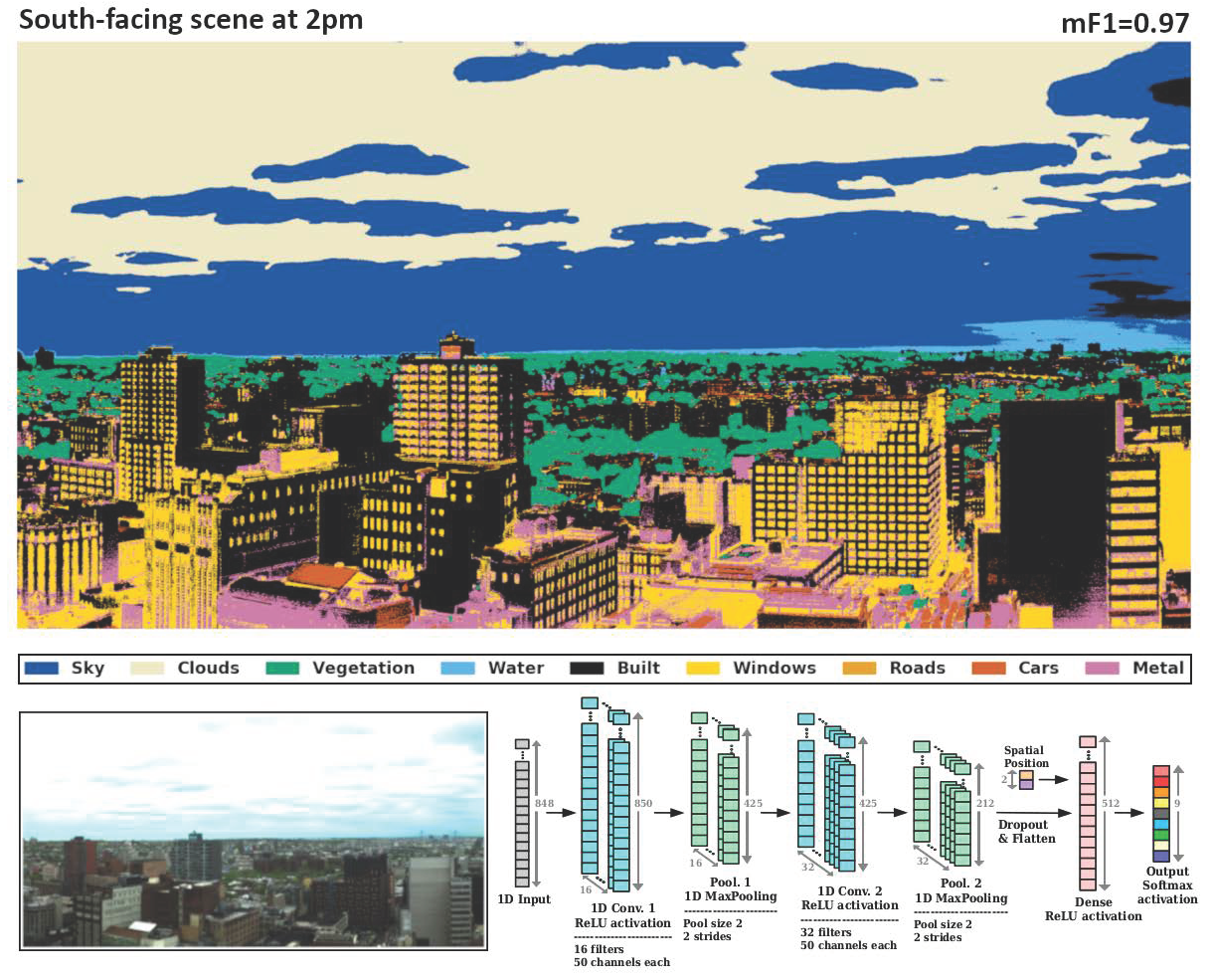
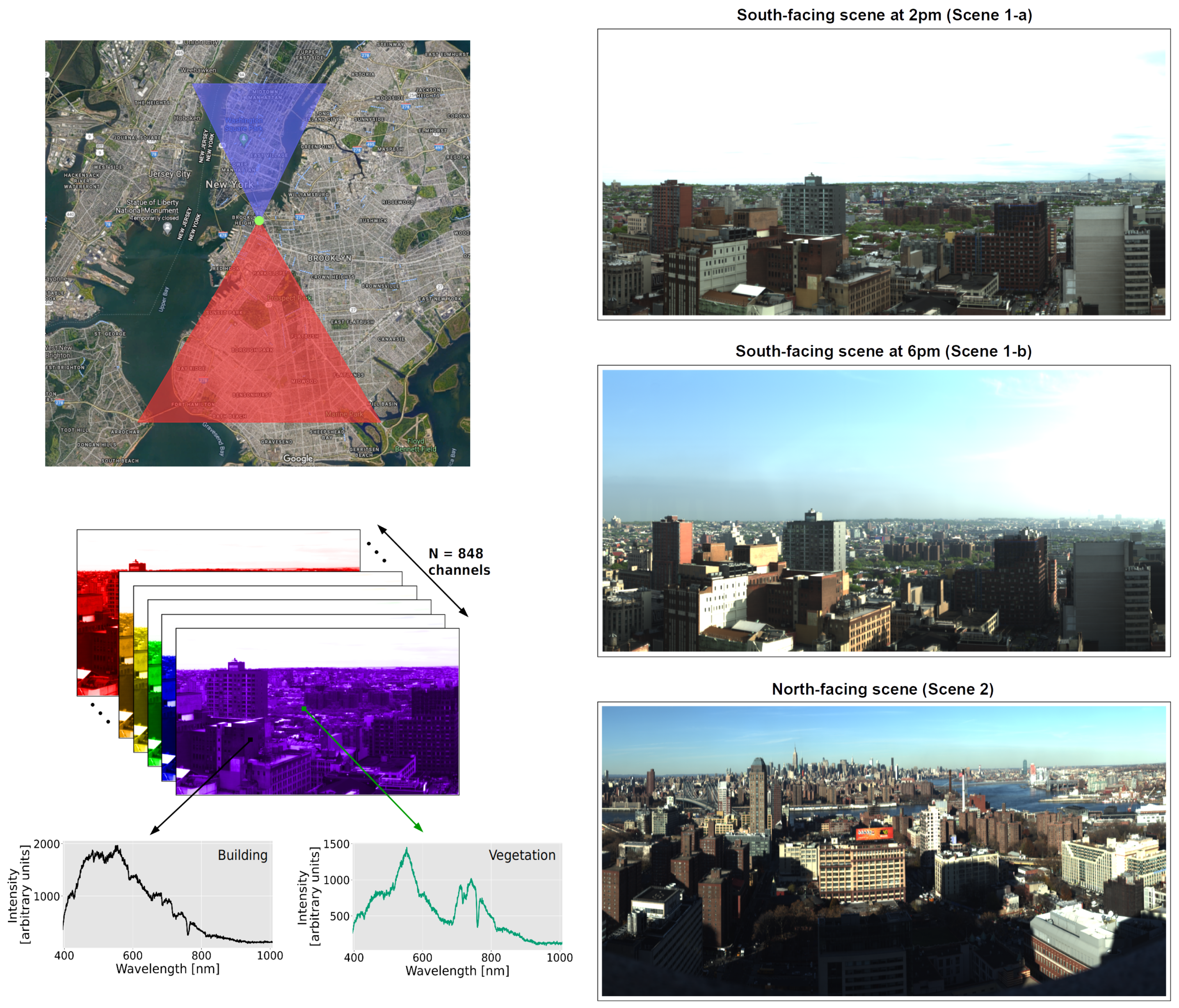
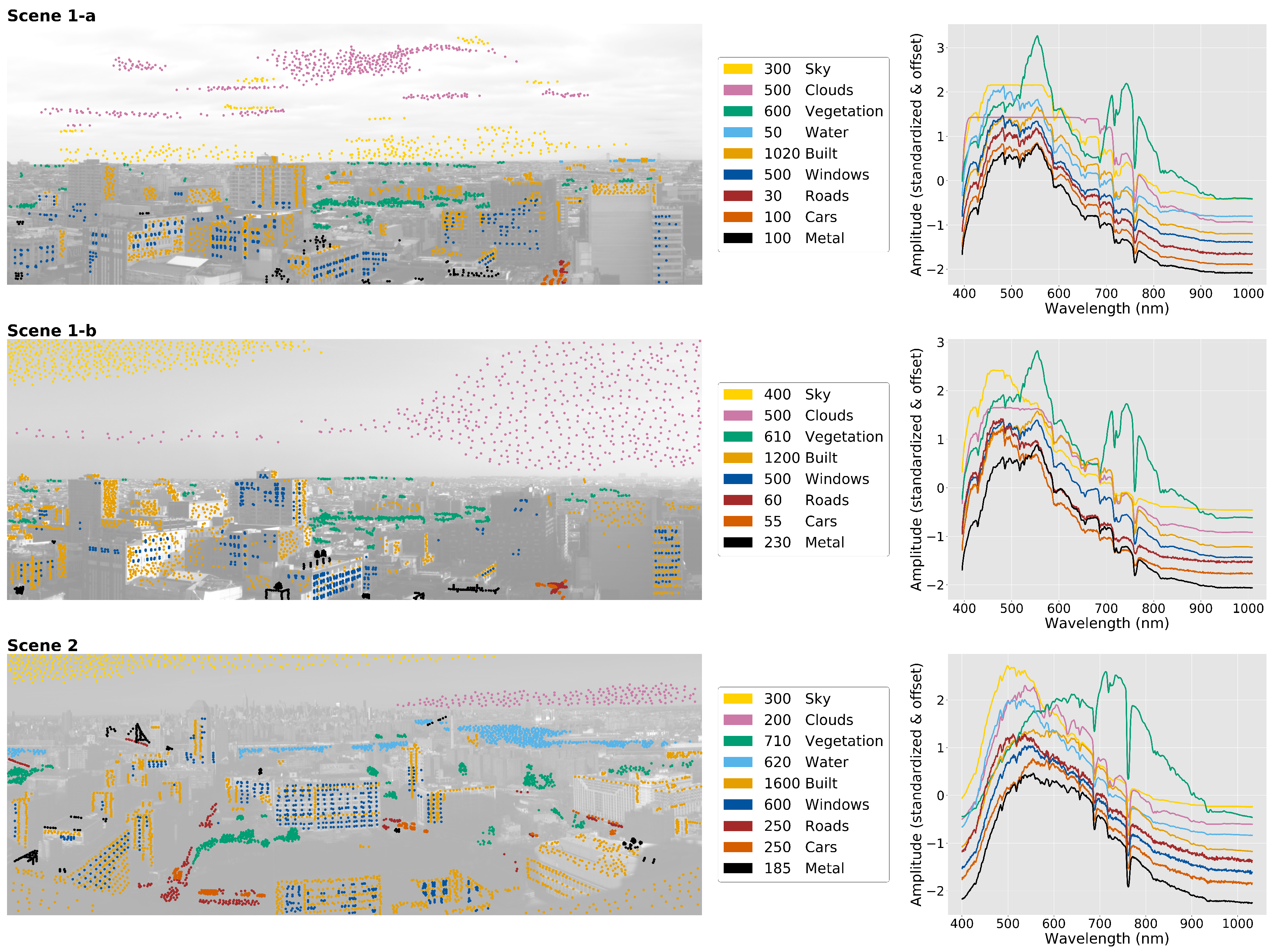
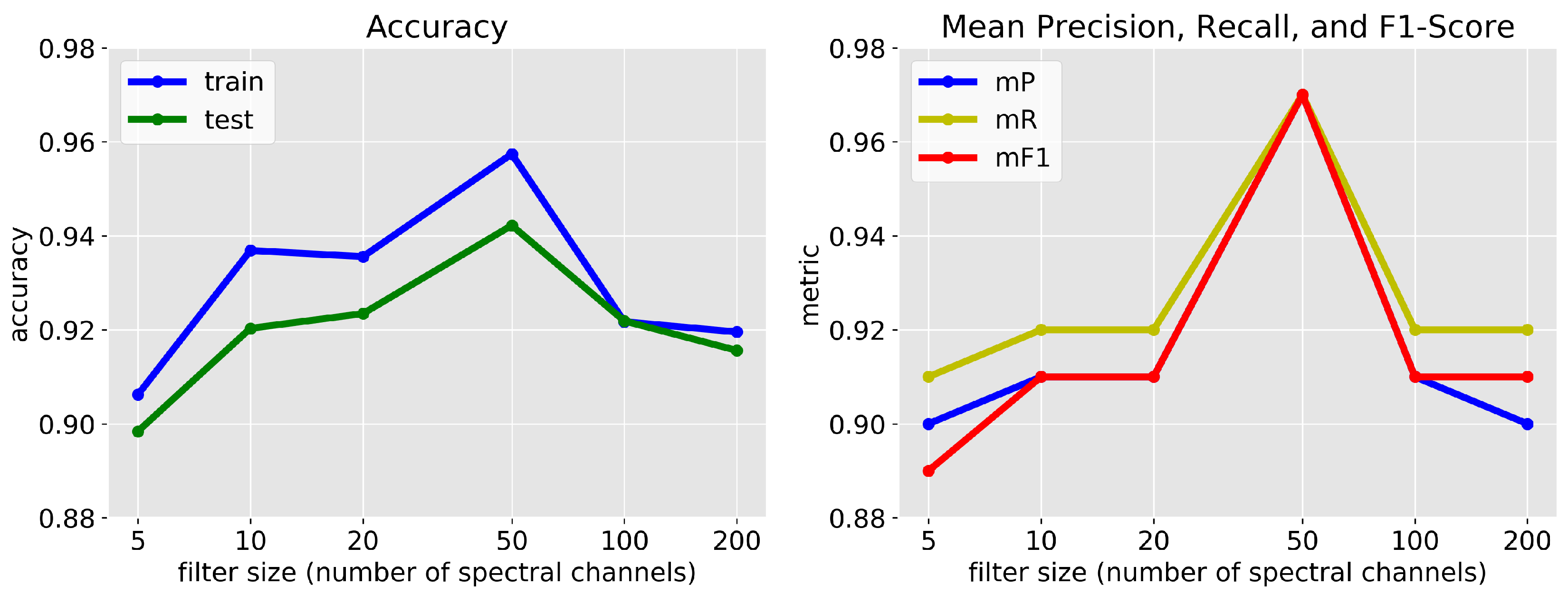
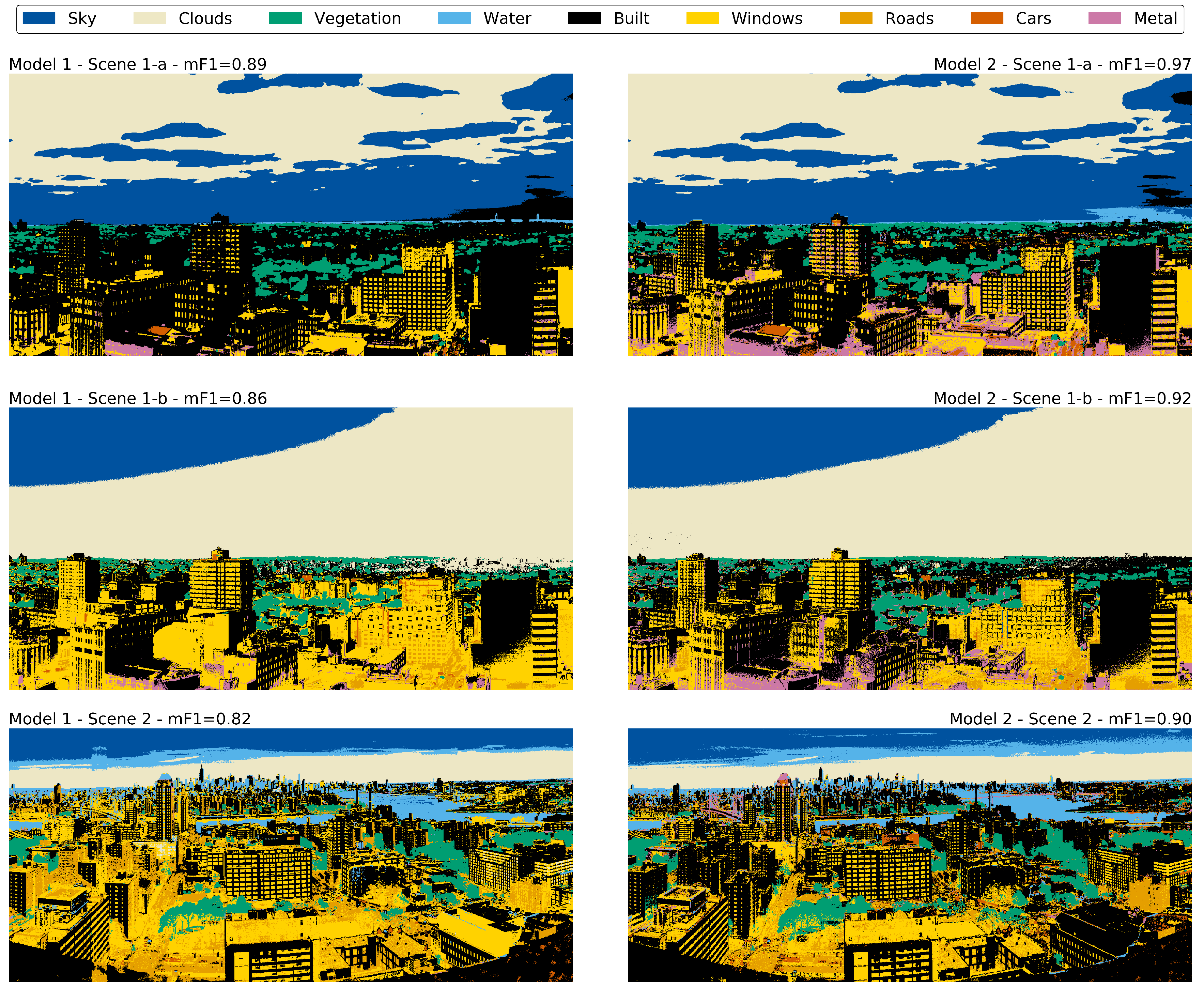
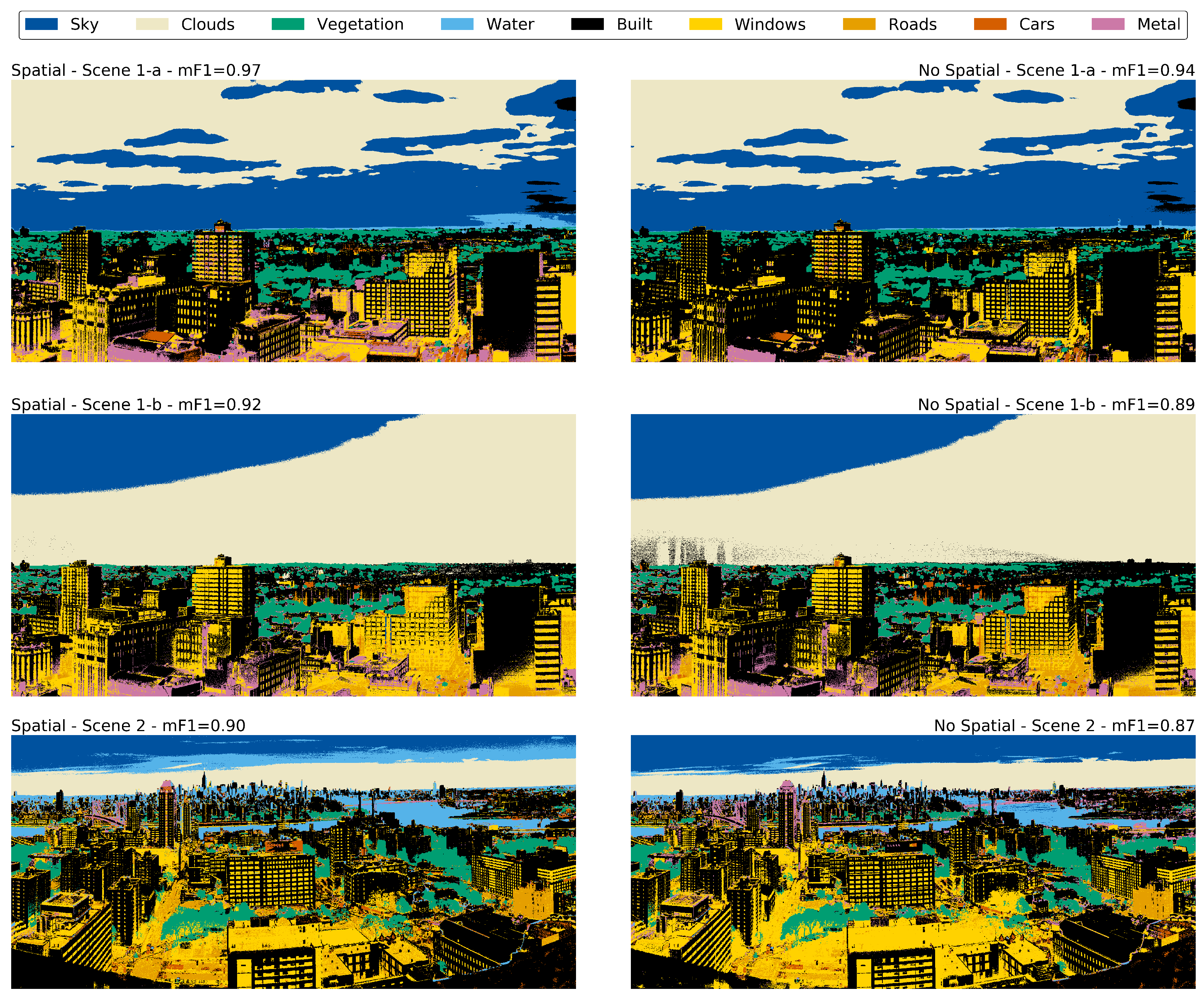
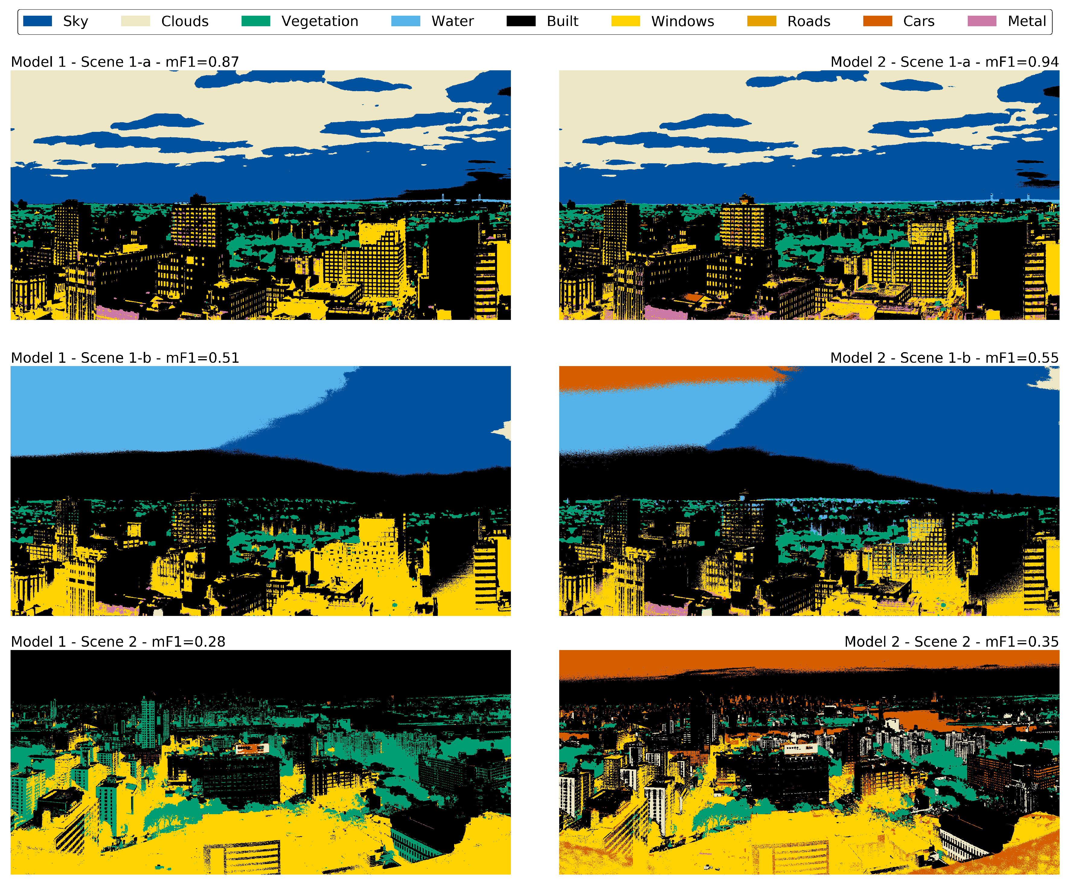
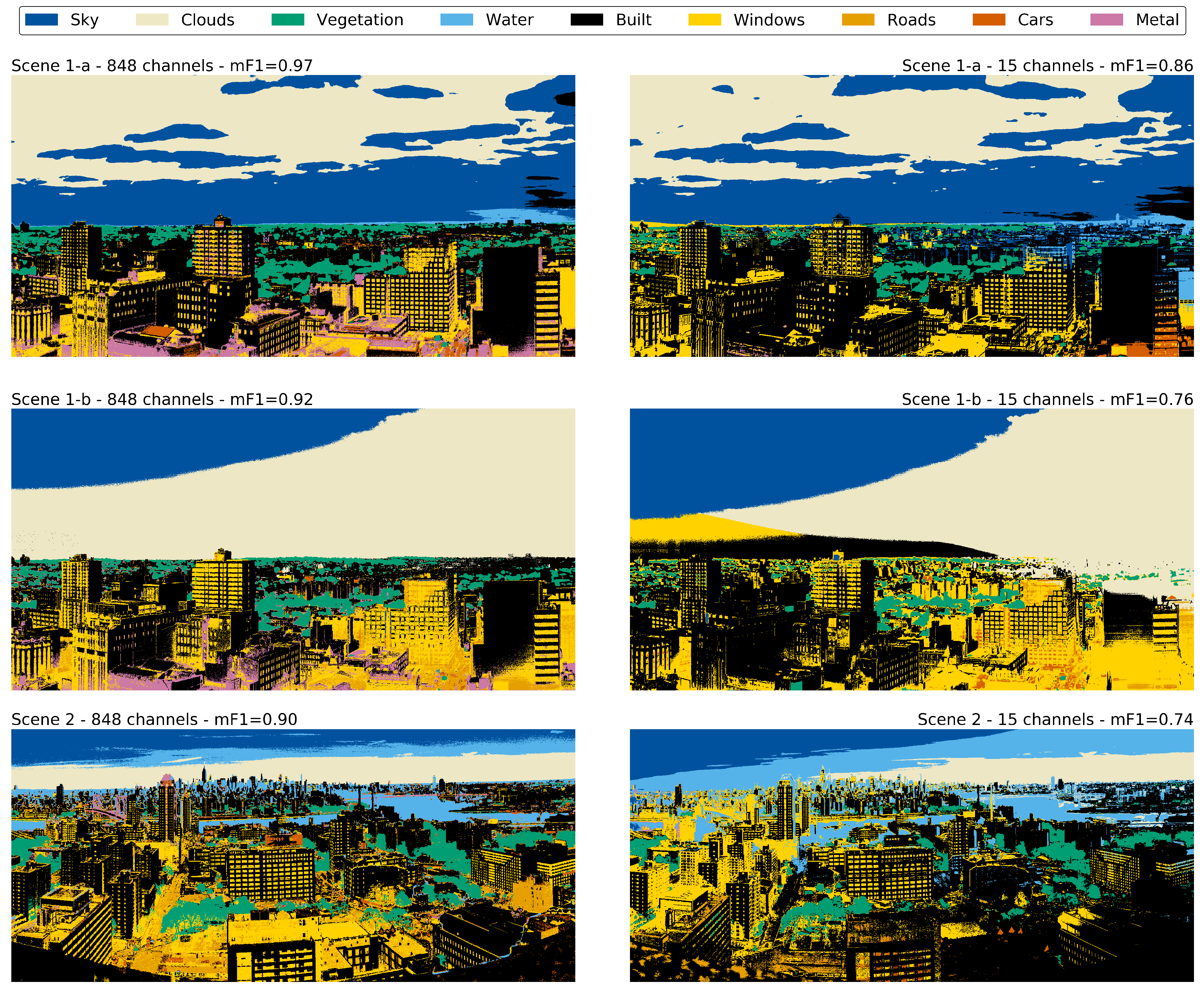
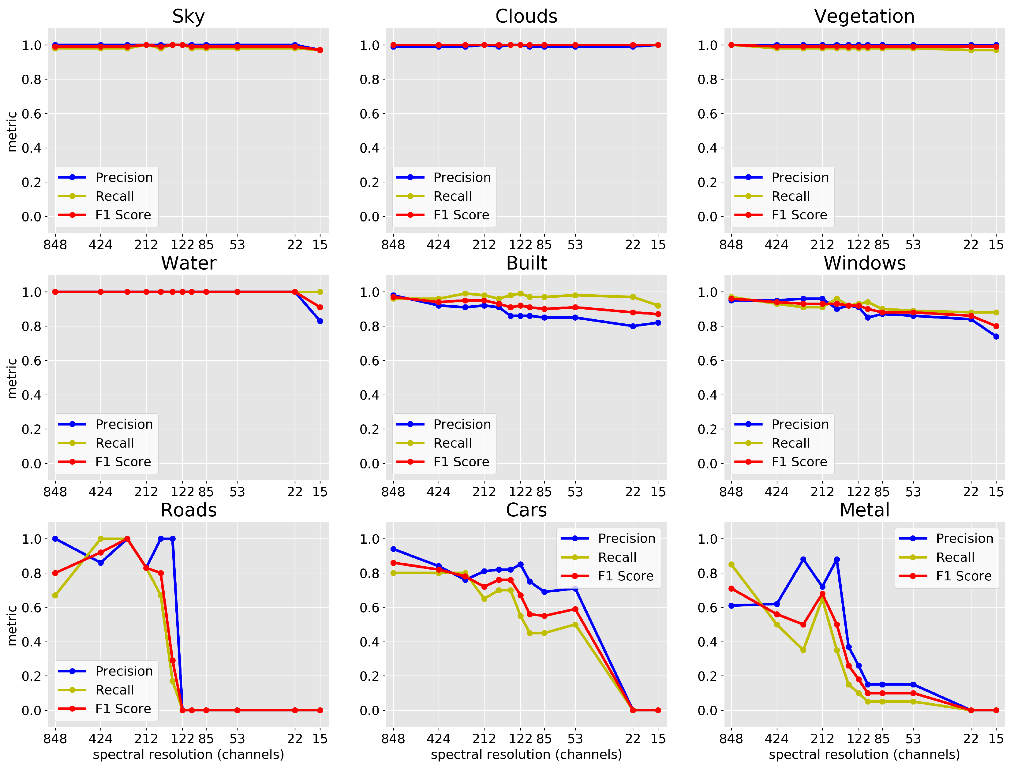
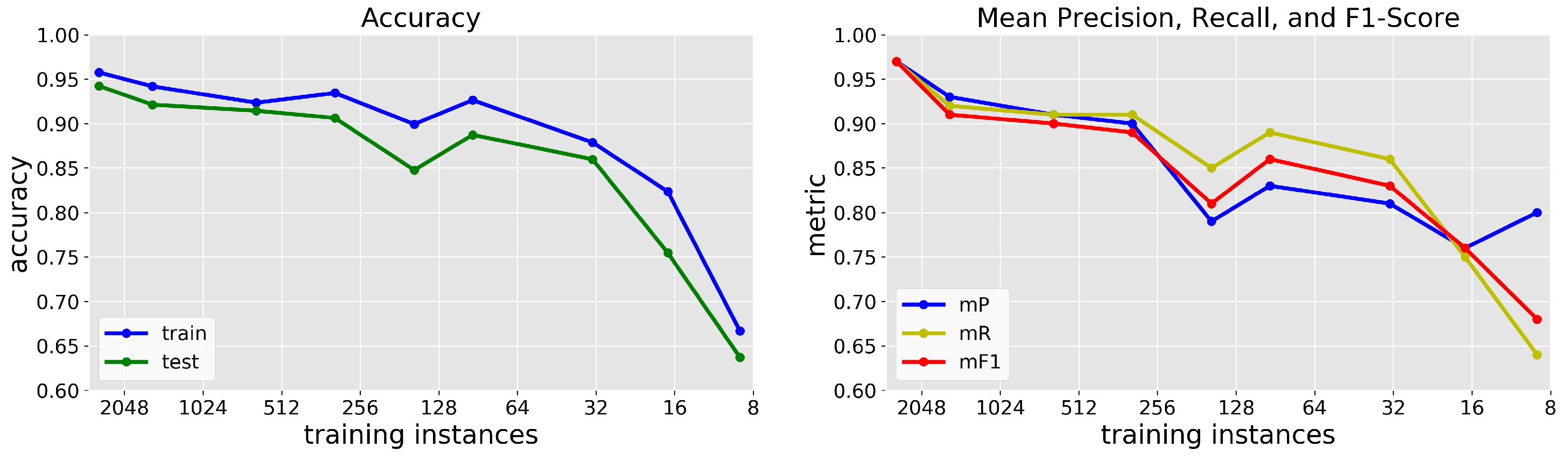
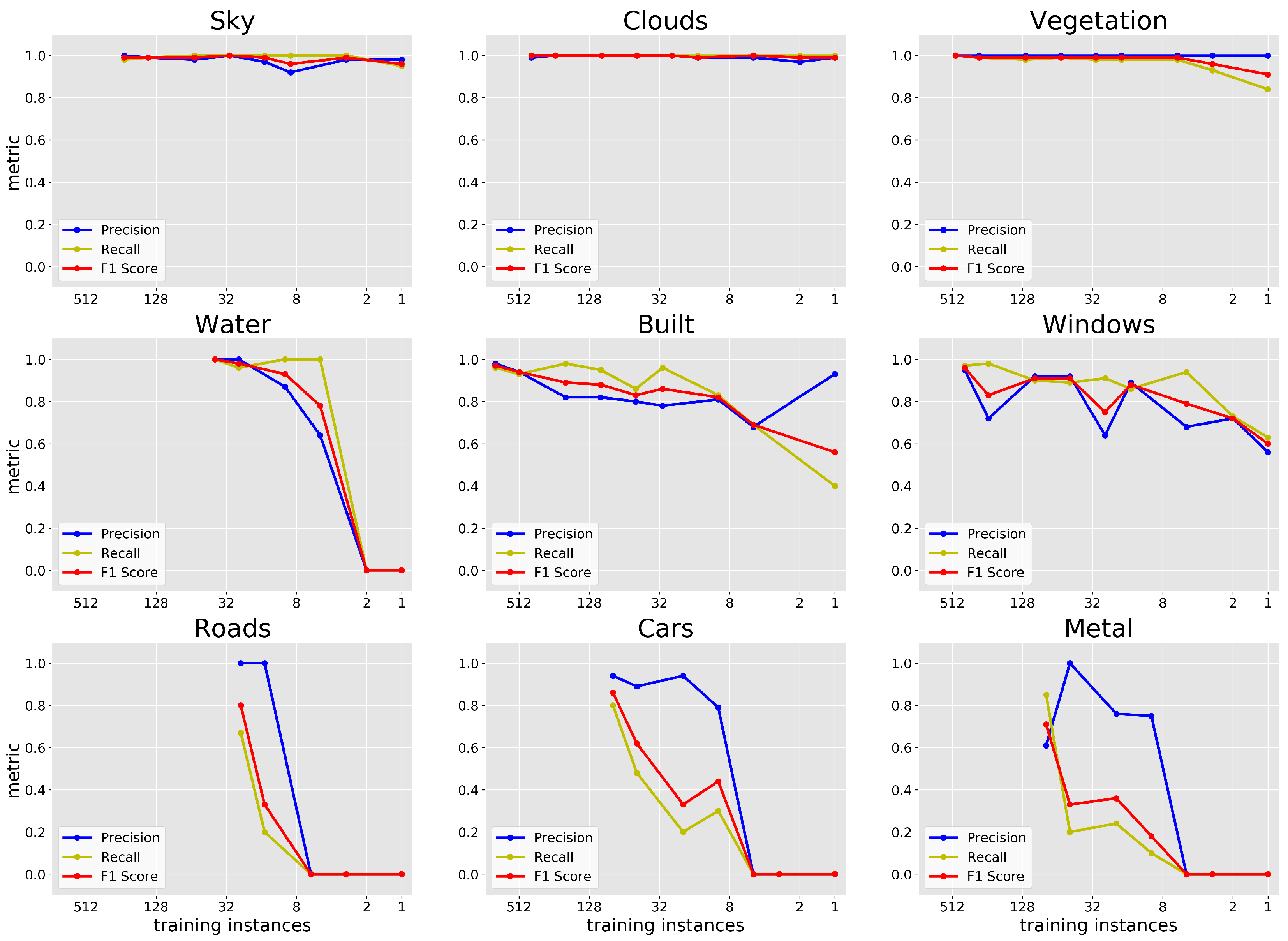
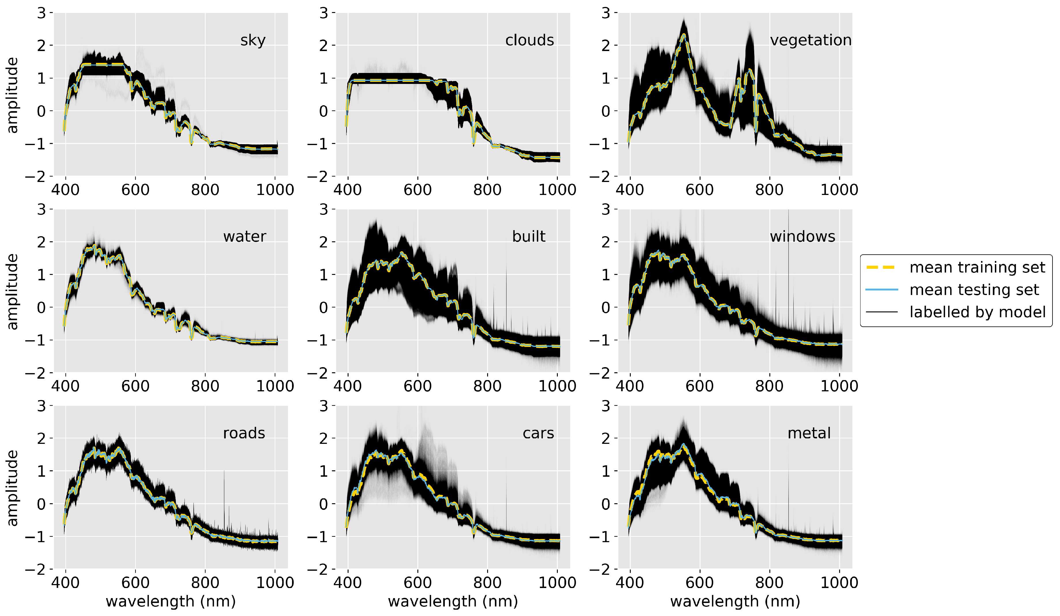
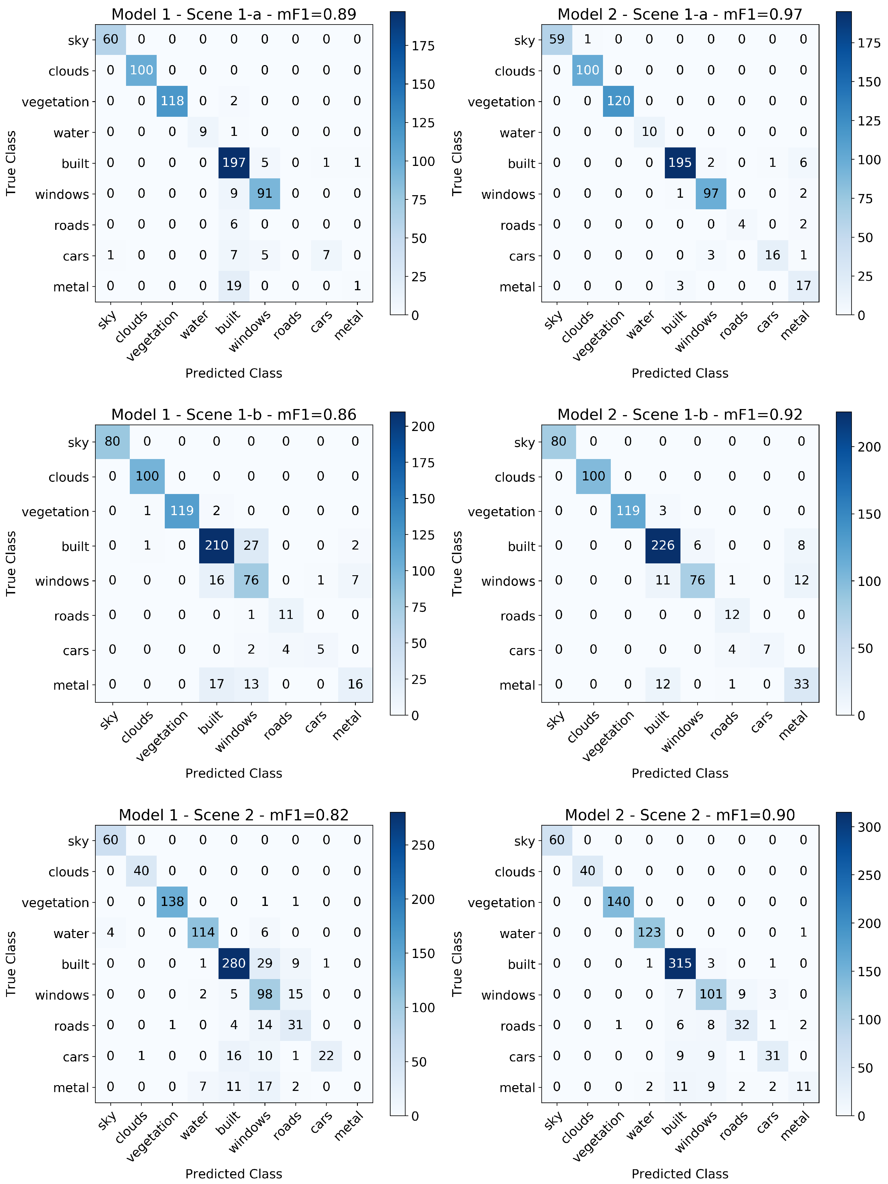
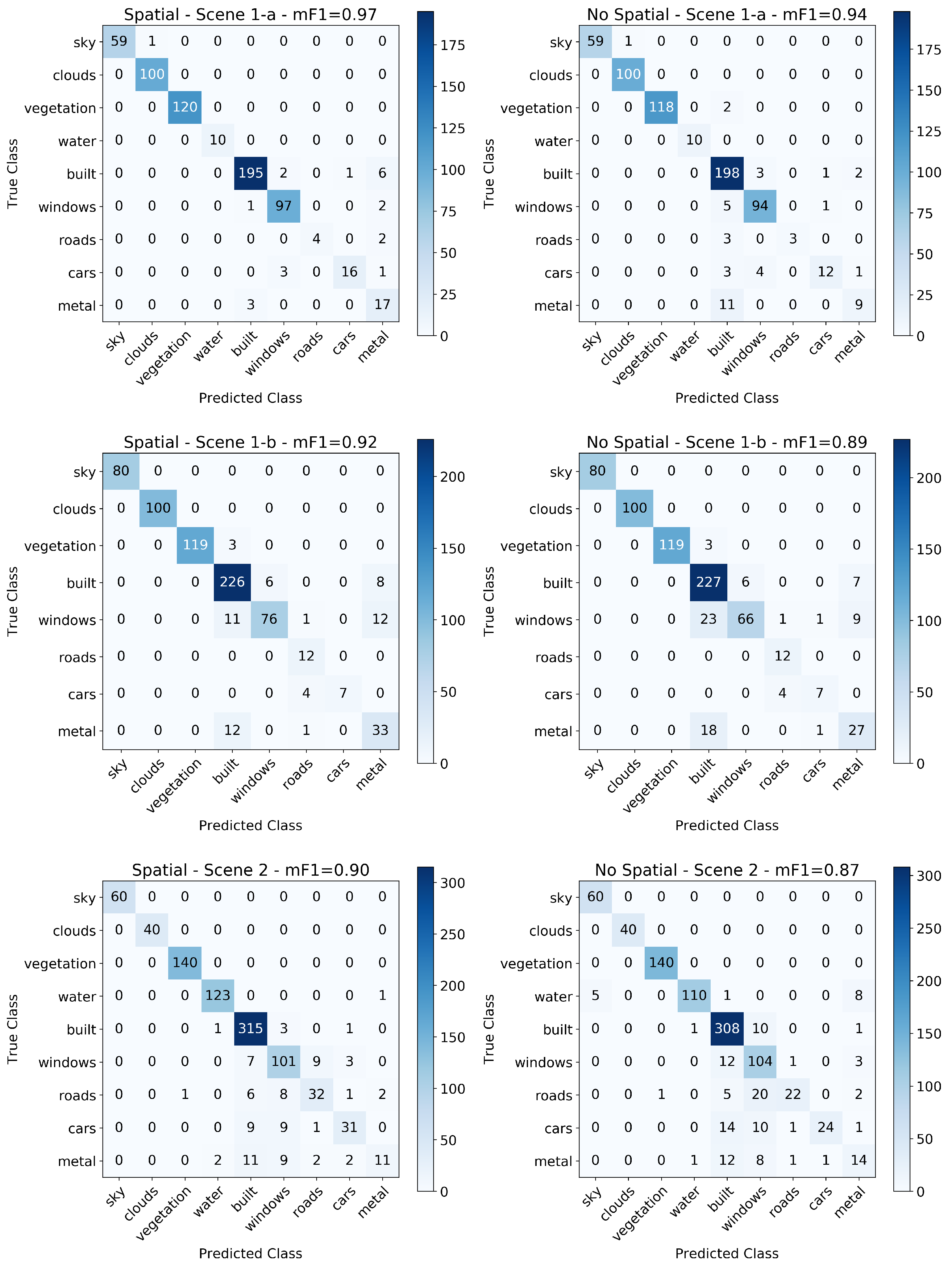
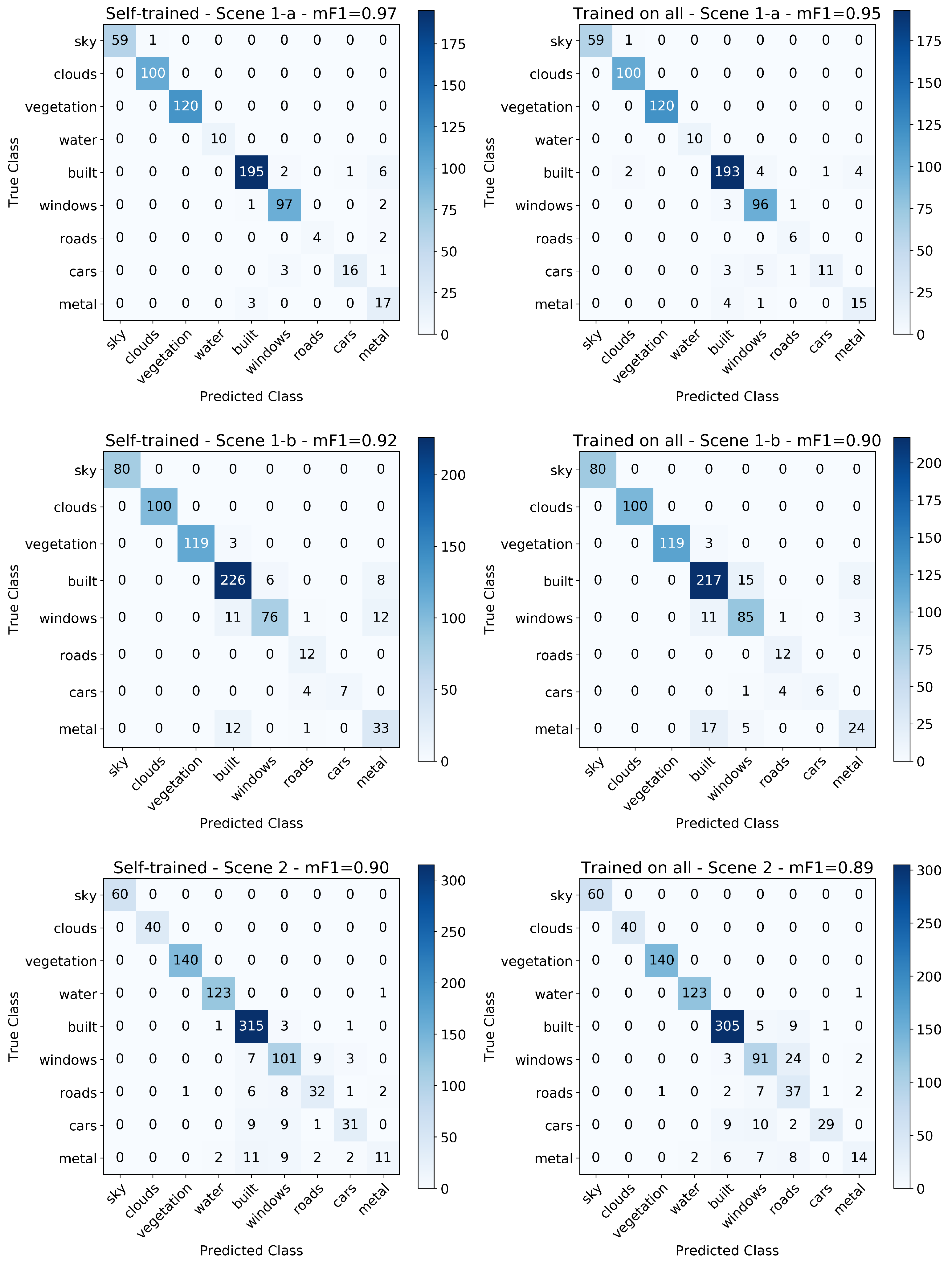
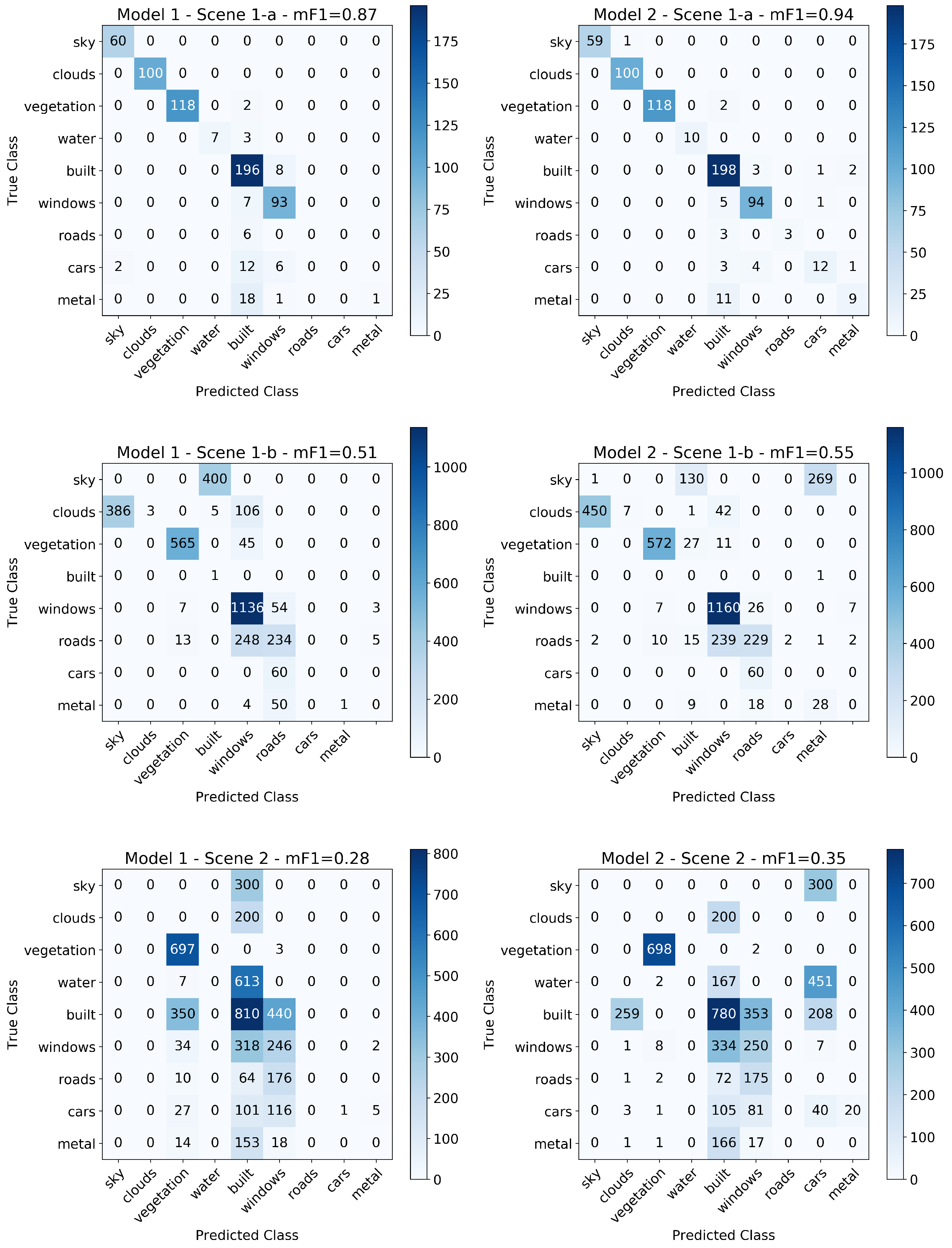
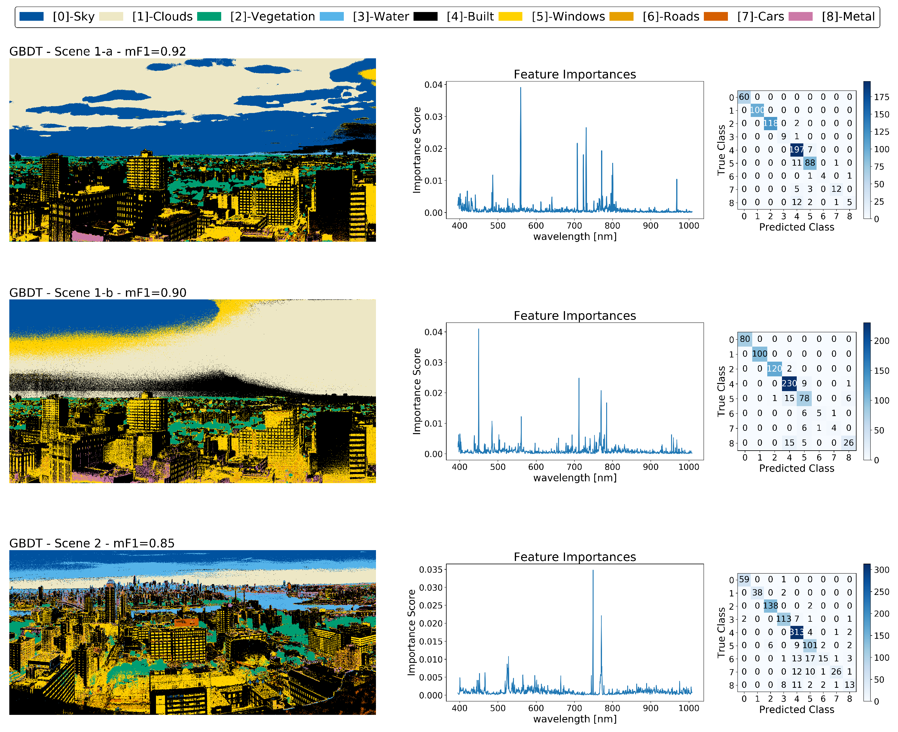
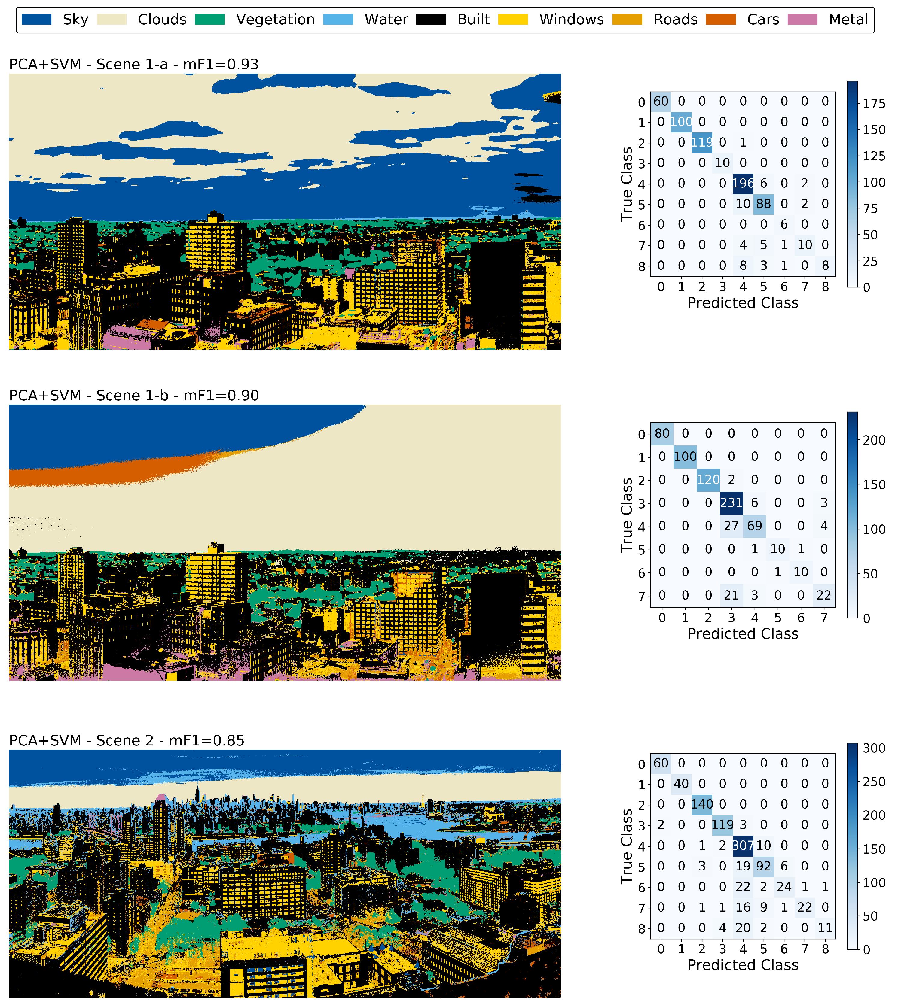
Table 1.
Performance metrics for the classification of hand-labeled pixel spectra with Model 1 and Model 2 (see Figure 4) computed from the confusion matrices provided in Appendix A Figure A1. Each model was trained and tested separately for each scene using only its own hand-labeled spectra. Comparisons between Model 1 and 2 are indicated with highlighted cells: dark highlighting indicates greater score by at least 5% and light highlighting indicates greater precision or recall by at least 5%. In general, Model 2 performed better at segmenting each scene than Model 1. In addition, Model 2 shows enhanced performance at classifying all human-built material pixels than Model 1, while both models performed well at classifying natural materials in all images.
| Performance Metrics: Models with Different Filter Sizes and Numbers Trained and Tested on Each Image Separately | ||||||||
|---|---|---|---|---|---|---|---|---|
| Model 1 | Model 2 | |||||||
| Image | Class | Support | Precision | Recall | Score | Precision | Recall | Score |
| Scene 1-a | Sky | 60 | 0.98 | 1.00 | 0.99 | 1.00 | 0.98 | 0.99 |
| Clouds | 100 | 1.00 | 1.00 | 1.00 | 0.99 | 1.00 | 1.00 | |
| Vegetation | 120 | 1.00 | 0.98 | 0.99 | 1.00 | 1.00 | 1.00 | |
| Water | 10 | 1.00 | 0.90 | 0.95 | 1.00 | 1.00 | 1.00 | |
| Built | 204 | 0.82 | 0.97 | 0.89 | 0.98 | 0.96 | 0.97 | |
| Windows | 100 | 0.90 | 0.91 | 0.91 | 0.95 | 0.97 | 0.96 | |
| Roads | 6 | 0.00 | 0.00 | 0.00 | 1.00 | 0.67 | 0.80 | |
| Cars | 20 | 0.88 | 0.35 | 0.50 | 0.94 | 0.80 | 0.86 | |
| Metal | 20 | 0.50 | 0.05 | 0.09 | 0.61 | 0.85 | 0.71 | |
| Total/Weighted Mean | 640 | 0.90 | 0.91 | 0.89 | 0.97 | 0.97 | 0.97 | |
| Scene 1-b | Sky | 80 | 1.00 | 1.00 | 1.00 | 1.00 | 1.00 | 1.00 |
| Clouds | 100 | 0.98 | 1.00 | 0.99 | 1.00 | 1.00 | 1.00 | |
| Vegetation | 122 | 1.00 | 0.98 | 0.99 | 1.00 | 0.98 | 0.99 | |
| Built | 240 | 0.86 | 0.88 | 0.87 | 0.90 | 0.94 | 0.92 | |
| Windows | 100 | 0.64 | 0.76 | 0.69 | 0.93 | 0.76 | 0.84 | |
| Roads | 12 | 0.73 | 0.92 | 0.81 | 0.67 | 1.00 | 0.80 | |
| Cars | 11 | 0.83 | 0.45 | 0.59 | 1.00 | 0.64 | 0.78 | |
| Metal | 46 | 0.64 | 0.35 | 0.45 | 0.62 | 0.72 | 0.67 | |
| Total/Weighted Mean | 711 | 0.87 | 0.87 | 0.86 | 0.92 | 0.92 | 0.92 | |
| Scene 2 | Sky | 60 | 0.94 | 1.00 | 0.97 | 1.00 | 1.00 | 1.00 |
| Clouds | 40 | 0.98 | 1.00 | 0.99 | 1.00 | 1.00 | 1.00 | |
| Vegetation | 140 | 0.99 | 0.99 | 0.99 | 0.99 | 1.00 | 1.00 | |
| Water | 124 | 0.92 | 0.92 | 0.92 | 0.98 | 0.99 | 0.98 | |
| Built | 320 | 0.89 | 0.88 | 0.88 | 0.91 | 0.98 | 0.94 | |
| Windows | 120 | 0.56 | 0.82 | 0.66 | 0.78 | 0.84 | 0.81 | |
| Roads | 50 | 0.53 | 0.62 | 0.57 | 0.73 | 0.64 | 0.68 | |
| Cars | 50 | 0.96 | 0.44 | 0.60 | 0.82 | 0.62 | 0.70 | |
| Metal | 37 | 0.00 | 0.00 | 0.00 | 0.79 | 0.30 | 0.43 | |
| Total/Weighted Mean | 941 | 0.82 | 0.83 | 0.82 | 0.90 | 0.91 | 0.90 | |
Table 2.
Performance metrics of CNN Model 2 both with and without pixel spatial information included for each of the three scenes in Figure 1, computed from the confusion matrices provided in Appendix A Figure A2. The cell highlighting is described in Table 1. Overall, the model variant with spatial information included outperformed that without when classifying the pixels in each scene. Both model variants performed better at classifying Scene 1-a than Scenes 1-b and 2. In particular, the model variant with spatial information included performed better at classifying the human-built structures in each scene, while both model variants had comparable performance in classifying the natural materials.
| Performance Metrics: Models with and Without Spatial Information Trained and Tested on Each Image Separately | ||||||||
|---|---|---|---|---|---|---|---|---|
| Spatial | No Spatial | |||||||
| Image | Class | Support | Precision | Recall | F 1 Score | Precision | Recall | F 1 Score |
| Scene 1-a | Sky | 60 | 1.00 | 0.98 | 0.99 | 1.00 | 0.98 | 0.99 |
| Clouds | 100 | 0.99 | 1.00 | 1.00 | 0.99 | 1.00 | 1.00 | |
| Vegetation | 120 | 1.00 | 1.00 | 1.00 | 1.00 | 0.98 | 0.99 | |
| Water | 10 | 1.00 | 1.00 | 1.00 | 1.00 | 1.00 | 1.00 | |
| Built | 204 | 0.98 | 0.96 | 0.97 | 0.89 | 0.97 | 0.93 | |
| Windows | 100 | 0.95 | 0.97 | 0.96 | 0.93 | 0.94 | 0.94 | |
| Roads | 6 | 1.00 | 0.67 | 0.80 | 1.00 | 0.50 | 0.67 | |
| Cars | 20 | 0.94 | 0.80 | 0.86 | 0.86 | 0.60 | 0.71 | |
| Metal | 20 | 0.61 | 0.85 | 0.71 | 0.75 | 0.45 | 0.56 | |
| Total/Weighted Mean | 640 | 0.97 | 0.97 | 0.97 | 0.94 | 0.94 | 0.94 | |
| Scene 1-b | Sky | 80 | 1.00 | 1.00 | 1.00 | 1.00 | 1.00 | 1.00 |
| Clouds | 100 | 1.00 | 1.00 | 1.00 | 1.00 | 1.00 | 1.00 | |
| Vegetation | 122 | 1.00 | 0.98 | 0.99 | 1.00 | 0.98 | 0.99 | |
| Built | 240 | 0.90 | 0.94 | 0.92 | 0.84 | 0.95 | 0.89 | |
| Windows | 100 | 0.93 | 0.76 | 0.84 | 0.92 | 0.66 | 0.77 | |
| Roads | 12 | 0.67 | 1.00 | 0.80 | 0.71 | 1.00 | 0.83 | |
| Cars | 11 | 1.00 | 0.64 | 0.78 | 0.78 | 0.64 | 0.70 | |
| Metal | 46 | 0.62 | 0.72 | 0.67 | 0.63 | 0.59 | 0.61 | |
| Total/Weighted Mean | 711 | 0.92 | 0.92 | 0.92 | 0.90 | 0.90 | 0.89 | |
| Scene 2 | Sky | 60 | 1.00 | 1.00 | 1.00 | 0.92 | 1.00 | 0.96 |
| Clouds | 40 | 1.00 | 1.00 | 1.00 | 1.00 | 1.00 | 1.00 | |
| Vegetation | 140 | 0.99 | 1.00 | 1.00 | 0.99 | 1.00 | 1.00 | |
| Water | 124 | 0.98 | 0.99 | 0.98 | 0.98 | 0.89 | 0.93 | |
| Built | 320 | 0.91 | 0.98 | 0.94 | 0.88 | 0.96 | 0.92 | |
| Windows | 120 | 0.78 | 0.84 | 0.81 | 0.68 | 0.87 | 0.76 | |
| Roads | 50 | 0.73 | 0.64 | 0.68 | 0.88 | 0.44 | 0.59 | |
| Cars | 50 | 0.82 | 0.62 | 0.70 | 0.96 | 0.48 | 0.64 | |
| Metal | 37 | 0.79 | 0.30 | 0.43 | 0.48 | 0.38 | 0.42 | |
| Total/Weighted Mean | 941 | 0.90 | 0.91 | 0.90 | 0.88 | 0.87 | 0.87 | |
Table 3.
Performance metrics of CNN Model 2 trained and tested on each of the three scenes in Figure 1 separately as opposed to CNN Model 2 trained on all scenes simultaneously. These metrics were computed from the confusion matrices provided in Appendix A Figure A3. The cell highlighting is described in Table 1. Overall, the two model variants (self-trained and all-trained) performed similarly in each scene, with the self-trained models marginally outperforming the all-trained model. In particular, both variants performed equally at classifying natural materials, but the self-trained models more accurately classified human-built materials.
| Performance Metrics: Trained and Tested on Each Image Separately vs. Trained on All Images Simultaneously and Tested on Each Image Separately | ||||||||
|---|---|---|---|---|---|---|---|---|
| Self-Trained and Tested | Trained on All | |||||||
| Image | Class | Support | Precision | Recall | F 1 Score | Precision | Recall | F 1 Score |
| Scene 1-a | Sky | 60 | 1.00 | 0.98 | 0.99 | 1.00 | 0.98 | 0.99 |
| Clouds | 100 | 0.99 | 1.00 | 1.00 | 0.97 | 1.00 | 0.99 | |
| Vegetation | 120 | 1.00 | 1.00 | 1.00 | 1.00 | 1.00 | 1.00 | |
| Water | 10 | 1.00 | 1.00 | 1.00 | 1.00 | 1.00 | 1.00 | |
| Built | 204 | 0.98 | 0.96 | 0.97 | 0.95 | 0.95 | 0.95 | |
| Windows | 100 | 0.95 | 0.97 | 0.96 | 0.91 | 0.96 | 0.93 | |
| Roads | 6 | 1.00 | 0.67 | 0.80 | 0.75 | 1.00 | 0.86 | |
| Cars | 20 | 0.94 | 0.80 | 0.86 | 0.92 | 0.55 | 0.69 | |
| Metal | 20 | 0.61 | 0.85 | 0.71 | 0.79 | 0.75 | 0.77 | |
| Total/Weighted Mean | 640 | 0.97 | 0.97 | 0.97 | 0.95 | 0.95 | 0.95 | |
| Scene 1-b | Sky | 80 | 1.00 | 1.00 | 1.00 | 1.00 | 1.00 | 1.00 |
| Clouds | 100 | 1.00 | 1.00 | 1.00 | 1.00 | 1.00 | 1.00 | |
| Vegetation | 122 | 1.00 | 0.98 | 0.99 | 1.00 | 0.98 | 0.99 | |
| Built | 240 | 0.90 | 0.94 | 0.92 | 0.88 | 0.90 | 0.89 | |
| Windows | 100 | 0.93 | 0.76 | 0.84 | 0.80 | 0.85 | 0.83 | |
| Roads | 12 | 0.67 | 1.00 | 0.80 | 0.71 | 1.00 | 0.83 | |
| Cars | 11 | 1.00 | 0.64 | 0.78 | 1.00 | 0.55 | 0.71 | |
| Metal | 46 | 0.62 | 0.72 | 0.67 | 0.69 | 0.52 | 0.59 | |
| Total/Weighted Mean | 711 | 0.92 | 0.92 | 0.92 | 0.90 | 0.90 | 0.90 | |
| Scene 2 | Sky | 60 | 1.00 | 1.00 | 1.00 | 1.00 | 1.00 | 1.00 |
| Clouds | 40 | 1.00 | 1.00 | 1.00 | 1.00 | 1.00 | 1.00 | |
| Vegetation | 140 | 0.99 | 1.00 | 1.00 | 0.99 | 1.00 | 1.00 | |
| Water | 124 | 0.98 | 0.99 | 0.98 | 0.98 | 0.99 | 0.99 | |
| Built | 320 | 0.91 | 0.98 | 0.94 | 0.94 | 0.95 | 0.95 | |
| Windows | 120 | 0.78 | 0.84 | 0.81 | 0.76 | 0.76 | 0.76 | |
| Roads | 50 | 0.73 | 0.64 | 0.68 | 0.46 | 0.74 | 0.57 | |
| Cars | 50 | 0.82 | 0.62 | 0.70 | 0.94 | 0.58 | 0.72 | |
| Metal | 37 | 0.79 | 0.30 | 0.43 | 0.74 | 0.38 | 0.50 | |
| Total/Weighted Mean | 941 | 0.90 | 0.91 | 0.90 | 0.90 | 0.89 | 0.89 | |
Table 4.
Performance of Model 1 and Model 2, trained on Scene 1-a and transferred to Scenes 1-b and 2, computed from the confusion matrices provided in Appendix A Figure A4. Highlighted cells compare results between the models with dark red highlighted cells indicating greater score by at least 5% and light red highlighted cells indicate greater precision or recall by at least 5%. In general, Model 2 shows enhanced performance over Model 1 when transferred to Scenes 1-b and 2; however both models performed significantly worse when transferred relative to training on each image separately. On a per class basis, Model 2 shows enhanced performance at classifying human-built structures than Model 1. The classification of Vegetation pixels remained consistently accurate and precise by both models in all testing cases. The inability of both models to classify any Sky and Clouds pixels in the transfer to Scene 1-b relative to their almost perfect classification in Table 1 is evidence of the significant dependence of illumination change on transfer performance.
| Performance Metrics: Transferring Models with Different Filter Sizes and Numbers Trained on Scene 1-a Tested on Scene 1-b and Scene 2 | ||||||||
|---|---|---|---|---|---|---|---|---|
| Model 1 | Model 2 | |||||||
| Image | Class | Support | Precision | Recall | F 1 Score | Precision | Recall | F 1 Score |
| Scene 1-a | Sky | 60 | 0.97 | 1.00 | 0.98 | 1.00 | 0.98 | 0.99 |
| Clouds | 100 | 1.00 | 1.00 | 1.00 | 0.99 | 1.00 | 1.00 | |
| Vegetation | 120 | 1.00 | 0.98 | 0.99 | 1.00 | 0.98 | 0.99 | |
| Water | 10 | 1.00 | 0.70 | 0.82 | 1.00 | 1.00 | 1.00 | |
| Built | 204 | 0.80 | 0.96 | 0.88 | 0.89 | 0.97 | 0.93 | |
| Windows | 100 | 0.86 | 0.93 | 0.89 | 0.93 | 0.94 | 0.94 | |
| Roads | 6 | 0.00 | 0.00 | 0.00 | 1.00 | 0.50 | 0.67 | |
| Cars | 20 | 0.00 | 0.00 | 0.00 | 0.86 | 0.60 | 0.71 | |
| Metal | 20 | 1.00 | 0.05 | 0.10 | 0.75 | 0.45 | 0.56 | |
| Total/Weighted Mean | 640 | 0.87 | 0.90 | 0.87 | 0.94 | 0.94 | 0.94 | |
| Scene 1-b | Sky | 400 | 0.00 | 0.00 | 0.00 | 0.00 | 0.00 | 0.00 |
| Clouds | 500 | 1.00 | 0.01 | 0.01 | 1.00 | 0.01 | 0.03 | |
| Vegetation | 610 | 0.97 | 0.93 | 0.95 | 0.97 | 0.94 | 0.95 | |
| Built | 1200 | 0.67 | 0.95 | 0.78 | 0.72 | 0.97 | 0.83 | |
| Windows | 500 | 0.53 | 0.47 | 0.50 | 0.65 | 0.46 | 0.54 | |
| Roads | 60 | 0.00 | 0.00 | 0.00 | 0.00 | 0.00 | 0.00 | |
| Cars | 55 | 1.00 | 0.02 | 0.04 | 0.09 | 0.51 | 0.16 | |
| Metal | 230 | 0.78 | 0.12 | 0.21 | 0.85 | 0.22 | 0.35 | |
| Total/Weighted Mean | 3555 | 0.67 | 0.55 | 0.51 | 0.70 | 0.58 | 0.55 | |
| Scene 2 | Sky | 300 | 0.00 | 0.00 | 0.00 | 0.00 | 0.00 | 0.00 |
| Clouds | 200 | 0.00 | 0.00 | 0.00 | 0.00 | 0.00 | 0.00 | |
| Vegetation | 700 | 0.61 | 1.00 | 0.76 | 0.98 | 1.00 | 0.99 | |
| Water | 620 | 0.00 | 0.00 | 0.00 | 0.00 | 0.00 | 0.00 | |
| Built | 1600 | 0.32 | 0.51 | 0.39 | 0.43 | 0.49 | 0.46 | |
| Windows | 600 | 0.25 | 0.41 | 0.31 | 0.28 | 0.42 | 0.34 | |
| Roads | 250 | 0.00 | 0.00 | 0.00 | 0.00 | 0.00 | 0.00 | |
| Cars | 250 | 1.00 | 0.00 | 0.01 | 0.04 | 0.16 | 0.06 | |
| Metal | 185 | 0.00 | 0.00 | 0.00 | 0.00 | 0.00 | 0.00 | |
| Total/Weighted Mean | 4705 | 0.28 | 0.37 | 0.28 | 0.33 | 0.38 | 0.35 | |
© 2020 by the authors. Licensee MDPI, Basel, Switzerland. This article is an open access article distributed under the terms and conditions of the Creative Commons Attribution (CC BY) license (http://creativecommons.org/licenses/by/4.0/).
Share and Cite
MDPI and ACS Style
Qamar, F.; Dobler, G. Pixel-Wise Classification of High-Resolution Ground-Based Urban Hyperspectral Images with Convolutional Neural Networks. Remote Sens. 2020, 12, 2540. https://0-doi-org.brum.beds.ac.uk/10.3390/rs12162540
AMA Style
Qamar F, Dobler G. Pixel-Wise Classification of High-Resolution Ground-Based Urban Hyperspectral Images with Convolutional Neural Networks. Remote Sensing. 2020; 12(16):2540. https://0-doi-org.brum.beds.ac.uk/10.3390/rs12162540
Chicago/Turabian StyleQamar, Farid, and Gregory Dobler. 2020. "Pixel-Wise Classification of High-Resolution Ground-Based Urban Hyperspectral Images with Convolutional Neural Networks" Remote Sensing 12, no. 16: 2540. https://0-doi-org.brum.beds.ac.uk/10.3390/rs12162540
Note that from the first issue of 2016, this journal uses article numbers instead of page numbers. See further details here.