An FPGA Accelerator for Real-Time Lossy Compression of Hyperspectral Images


1
Departamento de Arquitectura de Computadores y Automática, Facultad de Informática, Universidad Complutense de Madrid, 28040 Madrid, Spain
2
The Instituto de Tecnología del Conocimiento, University of Central Missouri, Warrensburg, MO 64093, USA
*
Author to whom correspondence should be addressed.
Remote Sens. 2020, 12(16), 2563; https://0-doi-org.brum.beds.ac.uk/10.3390/rs12162563
Submission received: 10 July 2020
/
Revised: 5 August 2020
/
Accepted: 6 August 2020
/
Published: 9 August 2020
(This article belongs to the Special Issue Remote Sensing Data Compression)
Abstract
:Hyperspectral images offer great possibilities for remote studies, but can be difficult to manage due to their size. Compression helps with storage and transmission, and many efforts have been made towards standardizing compression algorithms, especially in the lossless and near-lossless domains. For long term storage, lossy compression is also of interest, but its complexity has kept it away from real-time performance. In this paper, JYPEC, a lossy hyperspectral compression algorithm that combines PCA and JPEG2000, is accelerated using an FPGA. A tier 1 coder (a key step and the most time-consuming in JPEG2000 compression) was implemented in a heavily pipelined fashion. Results showed a performance comparable to that of existing 0.18 m CMOS implementations, all while keeping a small footprint on FPGA resources. This enabled the acceleration of the most complex step of JYPEC, bringing the total execution time below the real-time constraint.
1. Introduction
Remote sensing covers a broad range of techniques that are used to perform a variety of analyses remotely and with no close up interactions with the subjects of interest. Hyperspectral imaging is one of these techniques that has been growing since its inception.
It extends the concept of remote imaging by capturing information related not only to the visible part of the spectrum, but also in wavelengths that the human eye cannot see. A typical hyperspectral image will have from tens to hundreds of samples per pixel [1,2], each recording information of the light perceived at a specific wavelength.
The data collected at one wavelength are grouped in bands that span the whole image. The combination of multiple bands creates a spectral signature per pixel, providing information on a scale that helps with military applications such as target detection [3,4] and terrain trafficability [5], mineral identification [6,7], ground and water studies [8], vegetation and crop control [9,10], and many more.
It is the amount of information that is the bottleneck of hyperspectral imaging: storage and transmission are often limited in remote scenarios, and optimizing them is a must for uninterrupted image capture. Some of the most popular sensors such as EnMAP [11] reach speeds of 700 Mb/s and work uninterrupted for hours or days on a satellite.
Hyperspectral image compression has been explored in many ways, and has provided great results, especially in the lossless and near-lossless domains. Standards such as CCSDS [12] (a simple algorithm targeting on-board compression in real-time) have emerged for these applications. However, for long-term storage, a more powerful lossy algorithm is also of interest.
The literature has shown a variety of approaches, generally inspired by traditional image compression techniques. Predictive models ([13] Ch.2) have been optimized—even reordering bands ([13] Ch. 3) for increased correlation. Vector quantization (VQ) has also been extensively used to exploit pixel similarities [14]. Block-based approaches [15] have been used to reduce algorithm complexity. Wavelet techniques [16] have been extended from the 2D domain to anisotropic decompositions [17]. The most promising ones combine spectral decorrelation followed by compression in the spatial domain for each decorrelated band, using the Karhunen–Loève Transform ([18] Ch.9), or principal component analysis (PCA) [19].
The JYPEC algorithm [20] follows this approach by employing PCA as the decorrelation step, followed by JPEG2000 [21] as the spatial domain compressor. Since PCA decorrelates the most information-heavy bands first, variable bit-depths are used, thereby allocating more bits to the first components and using less bits for the ones that convey less information according to PCA (i.e., less variance).
This process is computationally intensive, and not suited for real-time in general purpose processors. When analyzed with care, the most intensive part has been found to be the JPEG2000 compression step, and more specifically, its encoder.
JPEG2000’s drawback is complexity, which is much higher [22] than that of the well-known and more extensively used JPEG [23]. The main reason is its block coding step, which takes up to 70% of the total execution time [24,25]. It includes simple operations but is heavy in conditional execution, making it unsuitable for traditional CPUs.
In order to level the playing field and bring lossy hyperspectral compression to real-time, acceleration techniques can be used. Field programmable gate arrays (FPGAs) offer a viable option with which to accomplish this task, and have been widely popular in accelerating block coding [24,26,27,28,29,30,31,32].
FPGAs each offer a reconfigurable fabric in which any circuit can be synthesized, and as a consequence have seen many applications [33,34]. They offer higher performance than a CPU or GPU, and the cost when compared to an ASIC is orders of magnitude smaller. They are also very efficient power-wise and radiation-hardened models [35] exist out of the box. All of these characteristics have made them very good candidates for remote sensing scenarios, wherein power is limited but performance and flexibility are still requirements. Great results have already been achieved for lossless and near-lossless hyperspectral image compression [36,37,38].
In [38] we present an FPGA implementation of the low complexity predictive lossy compression (LCPLC) algorithm. A highly pipelined architecture was designed which allows for real-time throughput while keeping FPGA usage low. However, when we want to obtain a very high compression ratio, the LCPLC algorithm does not obtain a distortion ratio as well as the JYPEC algorithm. Therefore in this study, JYPEC was accelerated using an FPGA. A tier 1 coder (a key step and the most time-consuming in JPEG2000 compression) was implemented in a heavily pipelined fashion. This enabled the acceleration of the most complex step of JYPEC, bringing the total execution time below the real-time constraint.
The rest of the paper is organized as follows: First, the JYPEC algorithm is looked at as a whole by detailing the tier 1 coder within JPEG2000, which was found to be the bottleneck for real-time execution. Secondly, an in-depth review of existing FPGA and ASIC implementations is presented, focusing on the different approaches for acceleration. Finally, a custom FPGA implementation of the tier 1 coder is presented based on the best techniques developed over the years, showing results that greatly improve on previous works, putting it in the context of real-time lossy hyperspectral image compression.
2. The JYPEC Algorithm
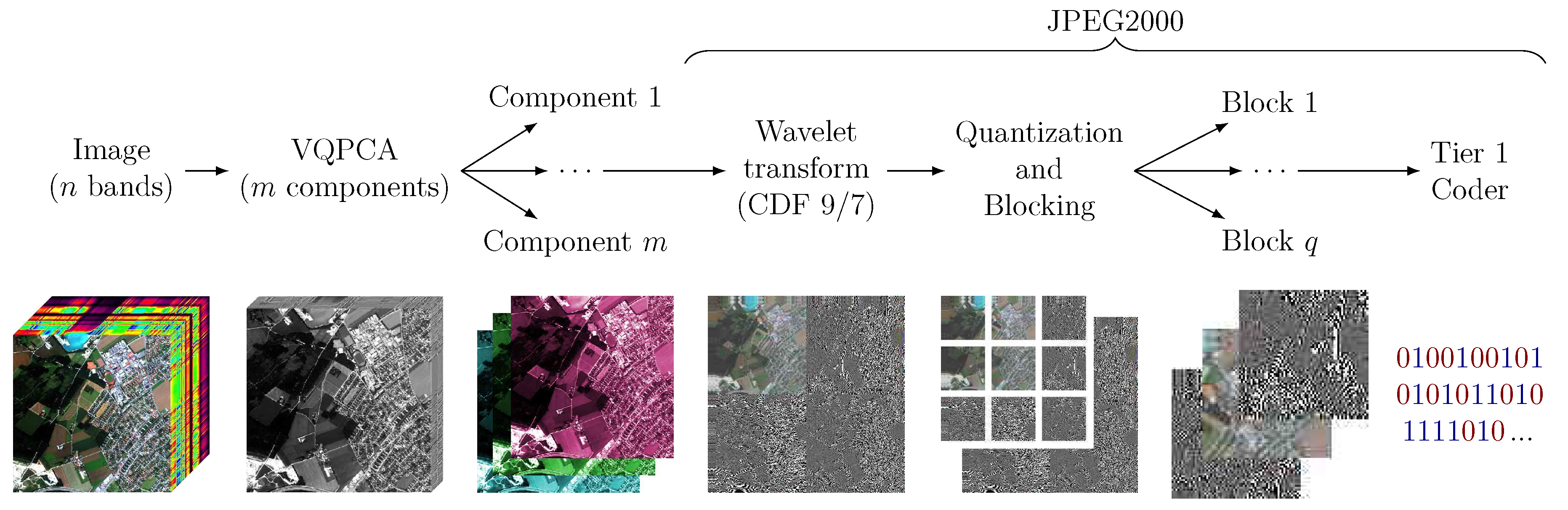
The JYPEC algorithm is a lossy algorithm aimed at hyperspectral image compression. It extends the concept presented in [19] of using PCA+JPEG2000 for compression. An optional vector quantization step is added prior to the dimensionality reduction, a variable bit-depth is used for each band, and the JPEG2000 coding is optimized for the whole image instead of for progressive decoding afterwards. This improves compression ratios and quality. A general diagram is seen in Figure 1.
2.1. Dimensionality Reduction
Even though JYPEC supports multiple dimensionality reduction algorithms, for this approach only PCA was used. It has a very low complexity (being a candidate for real-time), and has also a very good distortion-ratio performance [20], only falling short when targeting very high qualities at low ratios (against vector quantization PCA (VQPCA)).
First, a preprocessing step selects random pixels in the image. These pixels are processed by PCA, generating a set of vectors that indicate the directions of maximum variance within the set. Since the selection is random and the sample size is big due to the size of hyperspectral images, it matches well the total variance even when using only 1% of the total pixels [39]. This process generates a projection matrix to reduce the data size, as well as a recovery matrix to go back from the reduced data to the original size. Each band of the reduced image is compressed by JPEG2000.
The process can be undone by first uncompressing each reduced band, and then using the recovery matrix to project back into the original space.
2.2. The JPEG2000 Algorithm
The JPEG2000 standard is a multi-step algorithm which takes advantage of different image characteristics for compression. As well as being used for its main purpose of image compression, it has also found applications in compressing electroencephalography [40], video [41], and hyperspectral images [20], among others.
It follows a series of simple steps (Figure 2) to compress an image:
- A color transformation is done per pixel, converting the input color space (usually RGB) into a luminance (brightness) and chrominance (color) model, since human vision is more sensitive to brightness than color. The color channels can be down-sampled with no perceivable loss in quality, reducing a large chunk of the data bits.
- Every channel is then subjected to a wavelet transform [42]. A wavelet transform consists of a high-pass and a low-pass [43] filter that are applied both horizontally and vertically to all rows and columns respectively. This can be done in a reversible (lossless) or irreversible (lossy) way, and in either case the result is a partitioned channel in which different zones present different patterns that can be compressed to a higher degree than the original data.
- After doing the wavelet transform, the resulting values are quantized to integer values; some information is lost when the lossy wavelet transform is used.
- Finally, the values are encoded. The image is split into blocks of up to 4096 samples; each one is encoded individually, thereby exploiting local redundancies and the patterns left by the wavelet transform.
The color transform is not needed for hyperspectral compression, since the spectral dimension is already decorrelated by the dimensionality reduction step. Only the wavelet transform and encoding steps are performed.
The wavelet transform is fast when compared to encoding, which takes up to 70% of the total execution time [24,25] of JPEG2000. Within JYPEC, it also dominates execution times [39]. This paper focuses on a FPGA implementation that greatly improves encoding, bringing the full algorithm execution time down as much as possible by accelerating the bottleneck.
In the following subsections, the encoder algorithm is detailed to give a better understanding of the implemented accelerator later.
2.2.1. Encoding
Encoding is done in a lossless way over blocks of up to 4096 samples (usually squares, with a depth of 16 bits (15 magnitude + 1 sign). The encoding technique used in JPEG2000 is called embedded block coding with optimal truncation [44] (EBCOT). Two different coders lie within EBCOT: the tier 1 and tier 2 coders:
The tier 1 coder compresses the original block. The resulting stream has the prefix property: any prefix of that stream, once decoded, gives an approximation of the block. Longer prefixes provide better reconstruction accuracy.
The tier 2 coder splits the output streams from each block into sections, with each section refining the information decoded by the previous one. Sections from different blocks are interleaved by first storing the ones which better approximate the original image. This technique extends the concept of the prefix property from blocks to the full image. This part of the coder is not used here, since JYPEC targets full image compression and not progressive decoding.
2.2.2. Tier 1 Coder
Two phases lie within: First, the so called “bit plane coder” (BPC) pairs each bit with some context. This creates context—data pairs (CxD pairs). The distribution of all bits paired with the same context is highly skewed, making coding more efficient.
Second, CxD pairs are processed by the MQ-coder (it belongs to the family of arithmetic coders), generating the compressed output stream. The more skewed the input distributions are, the fewer bits the MQ-coder will output.
The BPC works by scanning the different bit planes of the block. First, the most significant bit of each sample is coded; then the second-most significant; and so on. This is the trick that later allows for progressive decoding.
The sign bit receives a special treatment, and is only coded when needed (i.e., when a sample is known to be nonzero, the sign bit for that sample is coded, but not before). This avoids coding sign bits for samples that are zero.
To exploit redundancies, bits are scanned in a zig-zag pattern in up to three passes per bit plane p (Figure 3). To keep track of what bit is scanned in what pass, a "significance" value is kept per sample , where j is the 2D position within the block/bit plane.
This value indicates whether a sample is significant (i.e., at least one of its already coded bits is one) or insignificant (if all bits have been zero up until the current pass in previous bit planes). A significant sample is either positive or negative depending on its sign bit.
Three distinct passes exist: First, a significance propagation pass in which bits from samples that are expected to turn significant in the current plane are coded. Second, a refinement pass that codes bits from all samples that are already significant. Finally, a cleanup pass that codes the remaining bits.
The cleanup pass will mostly code zeros and the significance pass will mostly code ones, while the refinement pass is more random. These skewed distributions are the key for compression. To increase efficiency, each bit is paired with a context based on the significance state of neighboring samples. The context is used to predict the value of the bit, and if right, can save even more space in the compressed stream.
The MQ-coder starts by mapping each context to two values:
- A bit x which is the current prediction for the given context.
- A state (of which there are 47 different ones) indicating the probability p of the prediction x being right.
The basic idea of the MQ-coder is that of arithmetic coders: The input data will be compressed as a subinterval . Starting with the interval , the data are subdivided with each CxD pair.
Given the probability p, is divided in and . If the predictive model is right, and the probability p high, (the bigger subinterval) will be kept. The bigger the final interval is, the less bits are needed to represent it.
In practice, infinite precision cannot be achieved, so 27 and 16 bits are allocated for c and a respectively as per JPEG2000 standard, calling them registers C and A.
Each state has an associated probability of finite precision mapping to the interval when dividing by , indicating the probability of its prediction’s success.
Since is fixed for a given state, its change is accomplished with two transition functions: most probable symbol (MPS) and least probably symbol (LPS). The MPS or LPS functions will be used depending on whether the prediction turns out to be right or not, and will change the state to one where is expected to better approximate the current bit input distribution. The prediction is also inverted when certain states are reached, doubling the possible states.
is used to update the interval by either adding to C or subtracting it from A. When both ends get close together, a shift left is performed to keep the length of the interval longer than the maximum value of .
A is kept under control by periodically resetting it, and C eventually overflows. The overflow is saved and forms the compressed output stream. To finish compression, C is flushed out. The process can then be reversed, and the original inputs recreated for decompression.
3. Existing Implementations
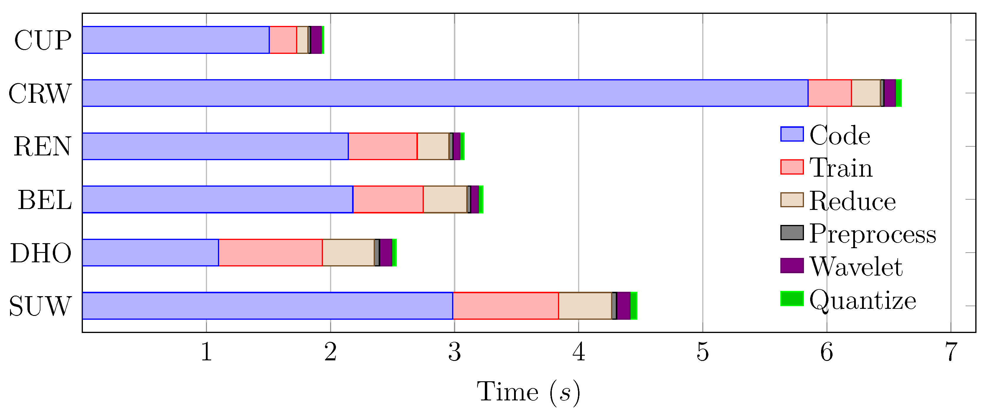
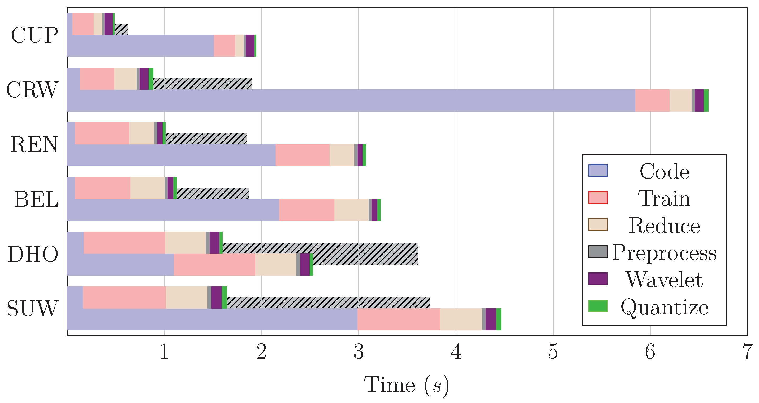
The objective of this study was to bring lossy compression to real time. For that, JYPEC was chosen as the target algorithm, and a tier 1 coder implementation of JPEG2000 (a step within JYPEC) is presented. It accelerates both the BPC and MQ-coder by making a single high-speed pipeline with both. To show that this effort was justified, a timing breakdown of compression of different images with JYPEC is shown in Figure 4.
It is clear that coding is the slowest part of the algorithm, and that any efforts to speed up the algorithm should be dedicated to it. Many implementations of the full tier 1 coder have been proposed, but more efforts have been focused towards accelerating the MQ-coder alone. In the following paragraphs, the literature is explored in this regard.
3.1. Bit Plane Coder
In [45], the authors designed a basic BPC which goes over the full block following the zig-zag pattern. Its controller is a 24 state machine which goes over the different passes bit by bit, producing at most one CxD pair per cycle.
Improving on that, in [25] the authors introduced the concept of skipping. They loaded full columns with four bits at once, and marked them with flags when they were no longer required in a certain pass. This way, the BPC could skip them when not needed, saving clock cycles. They also introduced flags for groups of columns and even full passes, allowing one to skip big chunks of idle cycles in some cases. Finally, since they loaded the full column at once, they also checked which bits needed to be encoded, and skipped the others within the column. In the end, savings of around of clock cycles were achieved.
A different approach was reported in [27]. Instead of skipping, the authors processed whole columns at once, producing up to 10 CxD pairs per cycle. CxD generation is not independent, so a series of cascading dependencies were taken into account. Despite the added complexity, this idea doubles the throughput of the sample-skipping technique without the extra memory. In [46], the authors went even further by allowing multiple planes to be coded simultaneously by using non-default coding options. Despite the small loss in compression efficiency, the throughput grew by a factor of 8 in CMOS 0.35 m technology when using gray-scale images. This, however, deviates from the standard implementation, since multiple MQ-coders would have had to be used for a single block in order to keep up with the BPC.
3.2. MQ-Coder
The MQ-coder has seen more optimizations [47] than the BPC, since traditionally the MQ-coder always was the bottleneck.
MQ-coder receives and processes CxD pairs from the bit plane coder, generating a compressed bit stream which can be further processed by the tier 2 coder. It is important to note that by design, the CxD pairs are processed serially, so no parallelization is possible at this stage.
Two main approaches have been used to accelerate its execution:
- Pipelining: As with many other designs, pipelining can be the key to improving performance. Distinct stages have been identified (mainly separating the update of A and C, and the output of coded byte(s)).
- Dual symbol processing: Some bit plane coders can produce two CxD pairs in one cycle. This has motivated the design of MQ coders with the capability of processing two pairs at the same time. Since this can not be done in parallel, these MQ-coders incorporate two cascaded processing units.
In [31], a three stage pipelined MQ coder is proposed. It performs all arithmetic operations in the first stage, A and C register shifts are done in a second stage, and a third stage emits bytes. The drawback of the authors’ approach was that the second stage could stall the first if the number of shifts was greater than one, since the authors did not use barrel shifters. In the end, they worked around this limitation by having two clock domains increasing the speed of the shifting stage, ensuring that stalling occurred only of the time, achieving a performance of around 145.9 MS/s on a Stratix EP1S10B672C6 board.
In [30], an implementation of the full tier 1 coder with no pipelining nor dual symbol processing is presented for the Virtex II Pro FG 456 board. They note that, at 112 MS/s, the arithmetic coder is the bottleneck, with the (context, bit) generation being five times faster. Speed was later increased by having up to four simultaneous instances of the tier 1 coder working in parallel.
In [48], two techniques were used to create a pipelined design that works at 413 MS/s: They first employed “traced pipelining” which consists of designing a pipeline for the most likely cases, and processing unlikely, more costly cases in a separate unit that stalls the pipeline if necessary. The second technique is based on eliminating cascading shifts (such as the ones from [29]) by looking ahead at the number of necessary shifts and performing them all at once. All of this is made possible by working on 0.18 m CMOS technology.
Both pipelining and dual processing are employed in the approach from [32], in which improvements are made to the multiple approaches from [26]. Dual processing is solved by having four different units processing all four possible scenarios (taking the lower or upper interval two times in any combination). Pipelining was used to separate the A register update, C register update, and byte output procedures, achieving in the end performances of 96.6 MS/s on FPGA and 440.2 MS/s on 0.18 m CMOS technology.
A different pipelined approach is presented in [49]. The A register update, C register update, and byte out procedures are kept in three distinct stages, and two more are added at the beginning by using two memory modules. The first one stores contextual information (namely state and predicted symbol) and the second one is a ROM which outputs state change information. If two consecutive contexts are equal, the second memory will be read with the updated state that is sent to the first one. This splits reading into a two-step process that accelerates the pipeline. The other notable technique is that shifting is limited to seven bits per cycle, reducing the critical path at the cost of one cycle stall in the unlikely case that the shift amount is greater than seven. In the end, a speed of 192.77 MS/s was achieved on 0.18 m technology.
4. Implementation
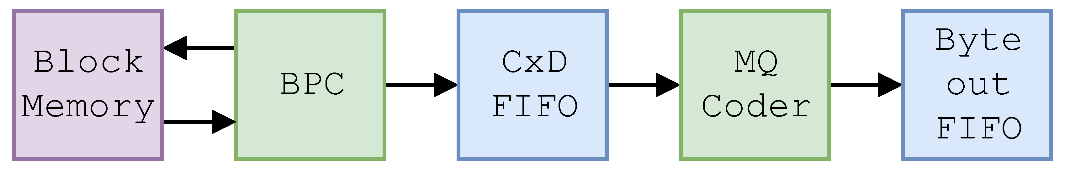
The presented design includes both the BPC and MQ-coder, chained together to form the full tier 1 coder. The basic structure of the tier 1 coder is shown in Figure 5.
The bit plane coder receives data from memory and generates CxD pairs. These are coded by the MQ-coder and the output stream is generated.
4.1. BPC
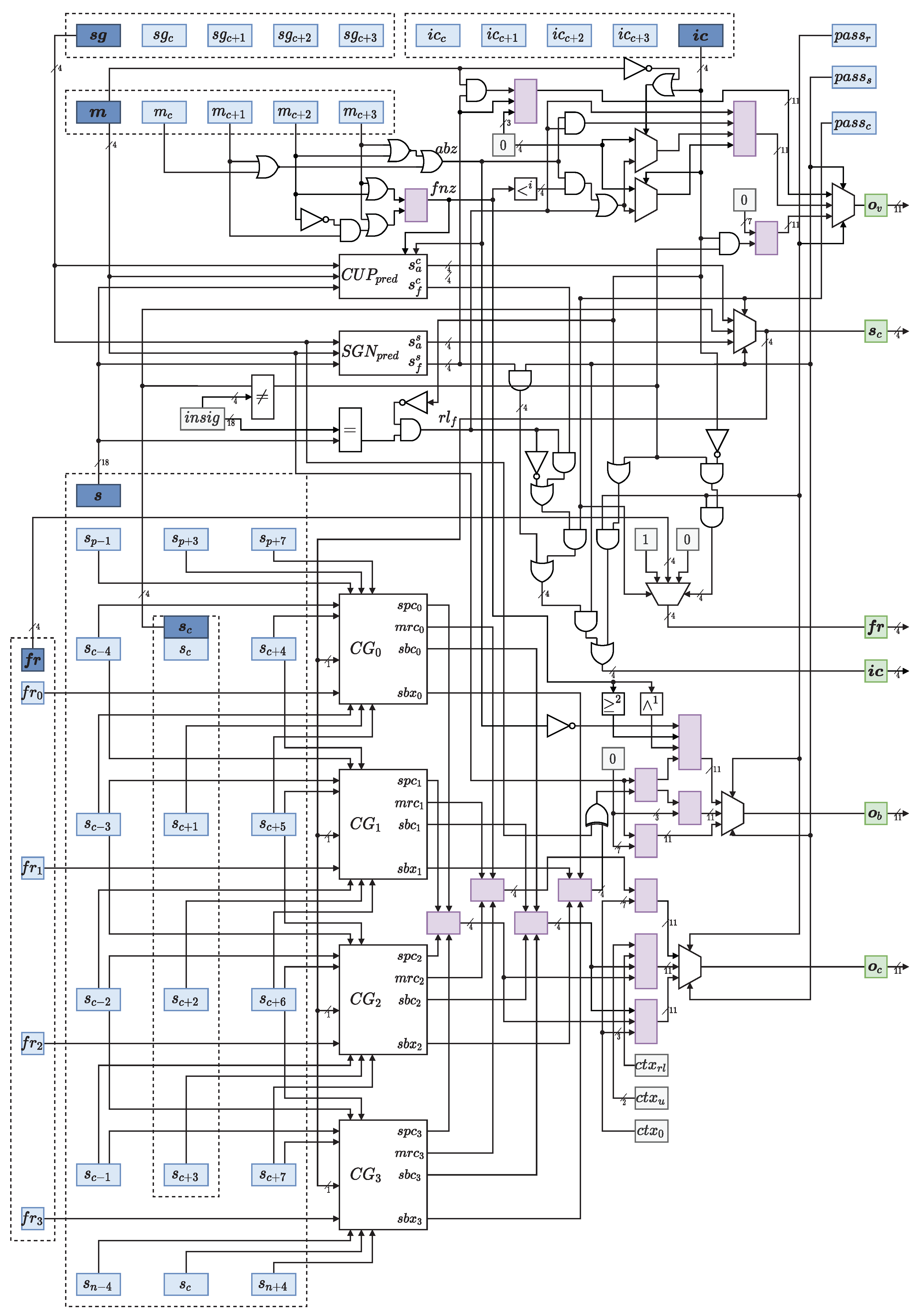
Internally, the BPC generates CxD pairs for four samples at a time (a full column of the zig-zag pattern), following the techniques of [27]. To generate the CxD pairs for a sample, flags from a neighborhood around the current sample are taken into account. When dealing with columns, this neighborhood grows to . This is seen in Figure 6.
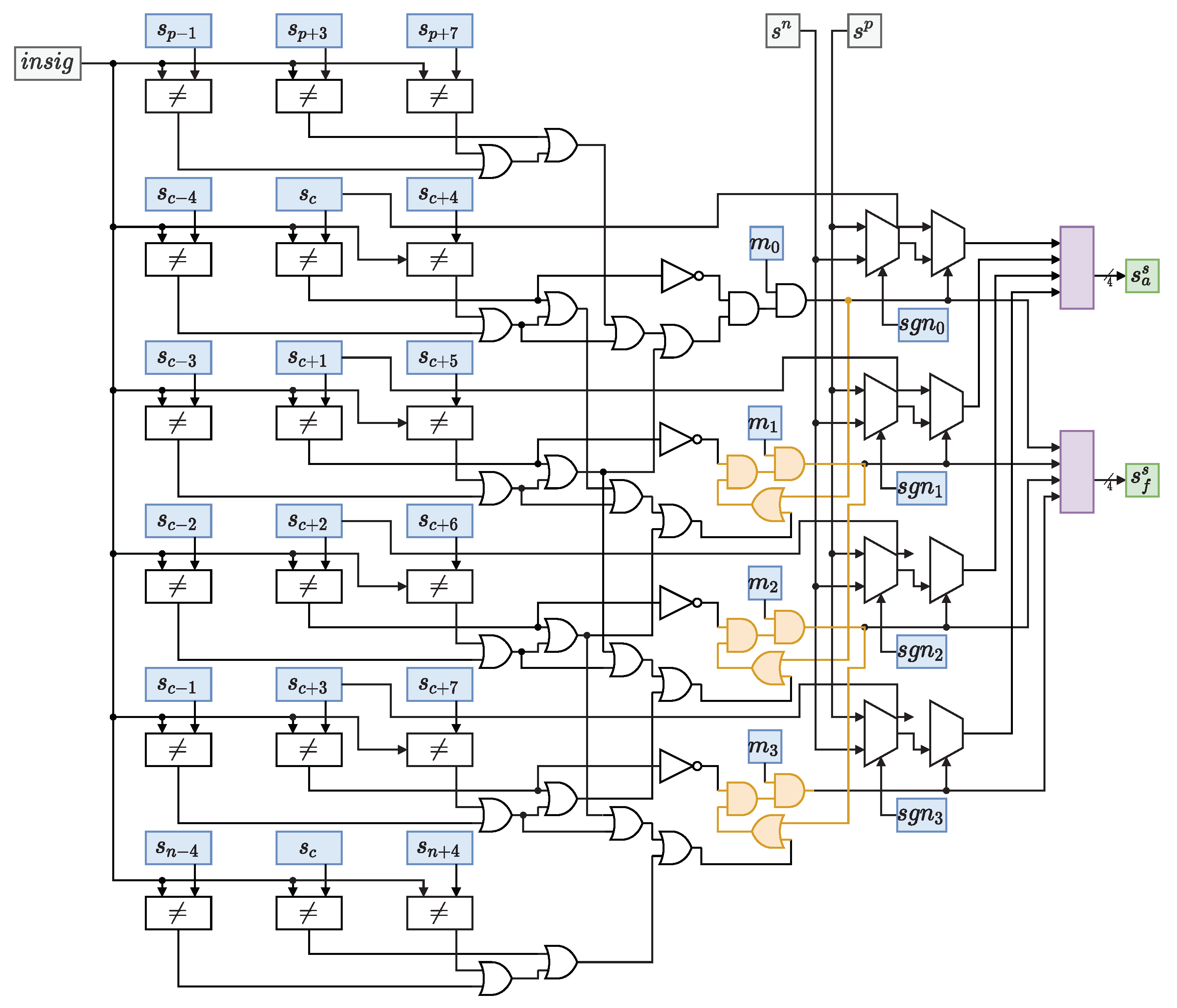
The main problem comes from the fact that the context generation modules are slow. They are based on lookup tables that require many LUT levels during FPGA implementation. They also need to be cascaded to generate the output significance that is required by the following bit strip. To avoid delays, a special module that predicts the next significance state in a faster way is used. It is shown in Figure 7.
The other modules are straightforward, with context generation being a ROM that outputs the context associated with the neighborhood by simple lookup. The cleanup predictor does a job similar to the significance predictor by looking at the first bit that is nonzero, and setting it and the following ones as significant if needed.
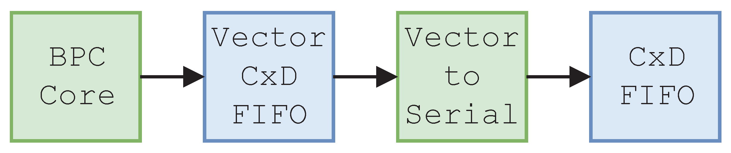
Up to 10 pairs are generated per cycle. A serializer is used to order them sequentially before sending them to the MQ-coder (see Figure 8).
With a big enough vector queue, the problem of running into idle cycles when few CxD pairs are generated is avoided (e.g., the first refinement pass or the last significance and cleanup passes), since a big enough buffer exists to keep feeding the MQ coder. The serializer is designed to output one pair per cycle as long as the vector queue is not empty, so it can feed the MQ-coder without forcing a stall.
4.2. MQ-Coder
The extensive work seen in Section 3.2 can be summed up in two different approaches: pipelining and dual-symbol processing. Since the target platform is an FPGA, pipelining is ideal to avoid a longer critical path which, on reconfigurable hardware, has a higher timing penalty than on fixed silicon. It will later be seen that a bottleneck arises in the CxD generation, so this area-efficient approach is the right choice since it can keep up with previous stages.
The only common step of all pipelining approaches is separating the byte out procedure in a last stage. Register updates are often split in two stages, treating A and C updates independently. Memory access is also split in some implementations. The point is, there are no obvious stages in the algorithm given the great dependency of the different stages. In fact, most designs implement the most likely execution path, having to stall in the event of an unexpected input.
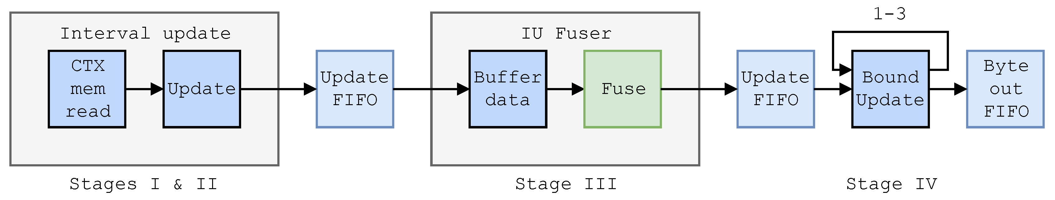
Most implementations are offering a theoretical throughput that varies depending on the data being compressed. The goal with this paper was to design an implementation which can consistently process CxD pairs at a certain speed. By pipelining the design and inserting queues in between stages, any potential stall in one stage gets absorbed by the queues and does not affect the others. The result can be seen on Figure 9.
Four main stages can be seen.
4.2.1. First and Second Stages
First, the context memory is accessed. This memory outputs “context information”, which has the prediction for that context, as well as the MPS and LPS transitions, XOR bit, and probability.
This memory is written with the context from the third stage, so care is taken whenever the same context is encountered twice in a three context window span:
- If the same context is found in cycles n and , a write–read cycle is skipped and input data are directly multiplexed to the memory’s output.
- To avoid stalling in the case where the same context appears in cycles n and , a second memory is present in the second stage, which outputs state information. The state is decided from the MPS and LPS transitions, and used to read this second memory. In this case, the context memory will be updated the next cycle. But those values are required in the current cycle, so a mux is used to bypass it from the second memory, avoiding a stall.
All in all, reading is segmented in two different stages, without the stalling that sometimes could happen in implementations such as [49].
The second stage is the most complex one, where the critical path lies. First, the context information to be used is decided, which comes from the context memory unless the same context appeared twice in a row, in which case it is fetched from the state memory and previous prediction.
State and prediction changes are fed to the state and context memories.
The prediction is adjusted, and the A register is updated. This can happen in one of four ways: either the A register is not shifted, it is shifted once or twice, or the contents are assigned from memory. In the last case, the number of shifts is calculated in advance.
The number of shifts , value to add to the C register, and hit flag h (indicating C needs to be updated with ) are sent to the next stage.
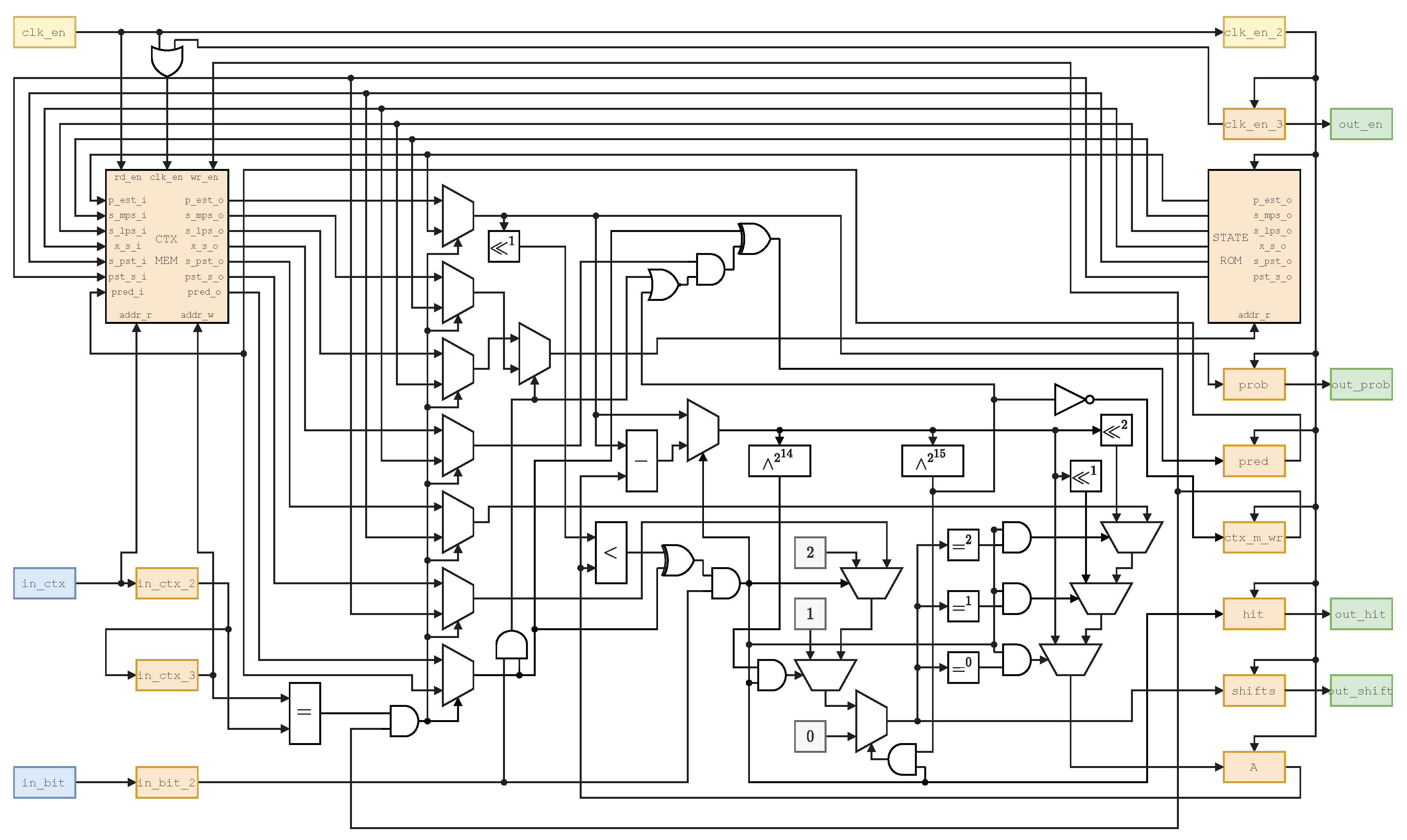
Both stages are seen in Figure 10.
4.2.2. Third Stage
The fourth stage can stall the pipeline. In order to minimize that risk, the inputs from multiple cycles are combined into just one update, so as to send the minimum number of updates ahead. This can be done under two scenarios:
- If and , both updates can be merged by setting , , . This merges two consecutive shifts that are under the maximum shift length of 15.
- If and , then both updates can be merged with , , . This is because the addition of to C happens before the shift . Both probabilities can be added at once because they are below the limit of .
Both these merging techniques can be done recursively.
4.2.3. Fourth Stage
The C register is updated by adding and shifting it. Whenever it fills up, a byte is output. When the register overflows or a special byte is output, padding needs to be added to avoid special markers used to indicate the end of stream. Up to three bytes might be output per update, and the control logic for all possibilities would make this stage too slow.
4.3. The Full Tier 1 Coder
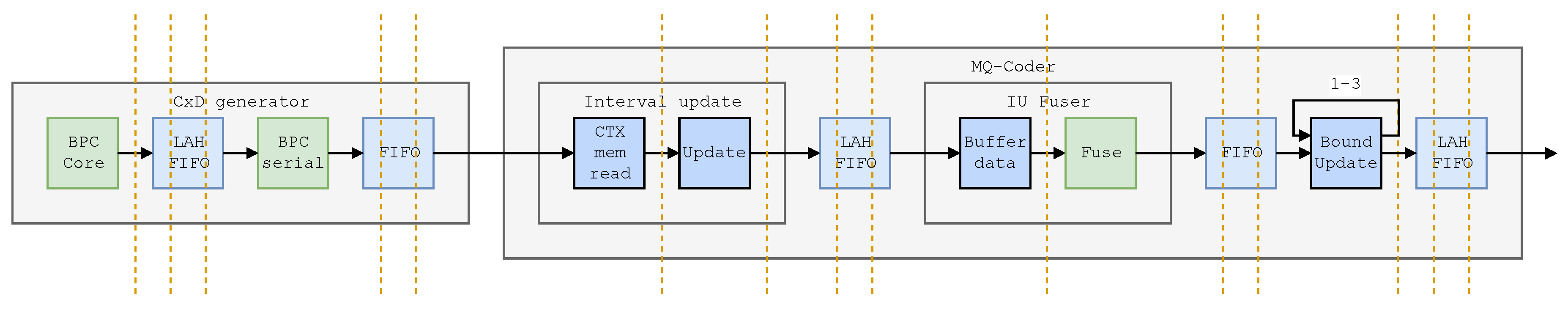
By chaining together both the BPC and MQ-coder, the tier 1 coder for JPEG2000 is formed. The basic segmentation is two stages for the BPC coder and four for the MQ-coder. Joining the different stages are multiple FIFOs. These help maintain a constant flow of data:
- When the MQ-coder stage IV stalls (because it has to output more than one byte), the fuser queue can hold updates until a fused one is sent (effectively canceling out the stalling).
- When the BPC-core is producing many CxD vectors, the vector queue avoids a stall from the BPC-core.
- Conversely, when the BPC-core does not produce vectors, the queue serves as a buffer to keep the next stages busy.
The full pipeline, taking into account the different queues, has a total of 15 stages, as seen in Figure 12. Despite the amount of stages, this has negligible impact in the final speed, since the coding of a full block takes a minimum of cycles, so filling the pipeline takes at most of the total cycles.
5. Results
The hardware architecture described in Section 4 has been implemented using VHDL language for the specification of the tier 1 coder. Moreover, we have used the 2020 Xilinx Vivado Design Suite environment to specify the complete system. The full system has been implemented on a VC709 board, a reconfigurable board with a single Virtex-7 XC7VX690T, two DDR3 SDRAM DIMM slots which hold up to 4 GB each, a RS232 port, and some additional components not used by our implementation. The HDLmodel has been verified via simulation and physical prototyping using a memory controller for input/output.
Table 1 shows the frequency and FPGA slice occupancy for the full tier 1 coder and its modules and submodules. More details are given in the following list:
- The BPC-core processes a full block of 65,536 bits in 44,032 cycles, working at a speed of 380 Mb/s.
- The BPC-serial can produce up to 390 MCxD pairs per second.
- The MQ-I/II stages processes 322 MCxD pairs per second, generating up to 322 M updates per second.
- The third stage is a bit faster, being able to merge 535 M updates per second.
- The last MQ stage processes up to 331 M updates per second.
- The intermediate FIFO queues have no problem at all keeping up with the speed requirements.
All in all, the full tier 1 coder is able to work at 255 MHz. At that speed, the bottleneck is the number of CxD pairs processed by the MQ-coder at 255 MCxD/s. By studying how many CxD pairs are produced, the input speed is calculated:
- The minimum number of updates for a block is seen when it is all zero, having successful run-length coding throughout the block. In this case, a total of = 15,360 updates are generated. That is, per bit.
- Conversely, an upper limit for the number of updates is given by a cleanup pass with run-length interruptions at every position, followed by 14 refinement passes. In this case, the number of updates is = 67,584 updates. Exactly per bit.
Thus, the input rate to generate 255 MS/s would range from 1.01 Gb/s to 247.3 Mb/s. However, the BPC-core is only capable of processing 380 Mb/s, so in practice this range is limited to 247.3 to 380 Mb/s.
The exact value within this range of course depends on the redundancy of the data. For [31], they compressed five images of size and noted that the average rate was . This means that, on average, the input rate for 255 MS/s would be 455 Mb/s. Thus it is safe to say that the tier 1 coder will consistently perform at its 380 Mb/s limit.
5.1. Comparison
A comparison with other implementations can be seen in Table 2. Only the best implementations found in the literature have been taken into account.
As seen, this implementation of the BPC works more than four times faster than other FPGA implementations, surpassing even ASIC designs in throughput.
With regard to the MQ-coder, this design doubles the performance of previous FPGA designs, only falling short of 0.18 m CMOS. It was expected that porting the design to this technology would make it faster than the competition, since other implementations have experienced [32] a speedup of 4× when doing so.
5.2. Acceleration of JYPEC
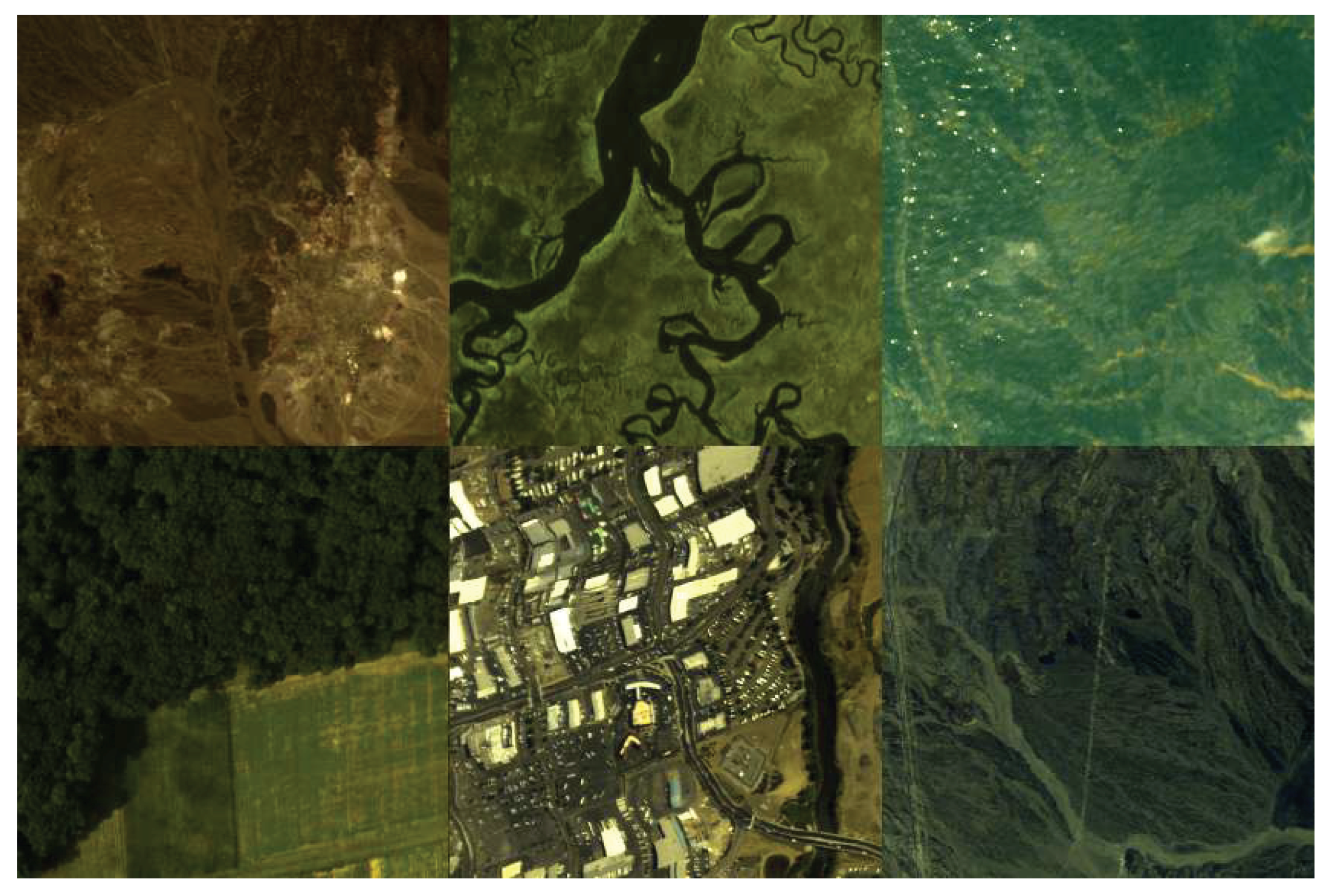
To see its impact on hyperspectral image compression under JYPEC, six images from two libraries have been compressed by JYPEC with and without acceleration. Four from the Spectir [55] library and two from the CCSDS 123 test data set [56]. The image characteristics are seen in Table 3 and a preview in Figure 13.
The results have been acquired in a DELL XPS 13 9360 computer, with an i7-7500U processor with a thermal design power (TDP) of 15 W, 8 GB of RAM running at 1866 MHz, and 256 GB of SSD PCIe storage. For the accelerated version, the time of coding in the processor was replaced with the time of coding in the FPGA itself. Memory transfer times ertr not taken into account, because the PCIe of the VC709 board works at 25 GB/s and the typical image size is 500 MB, so it was transferred in 20 ms, not impacting results.
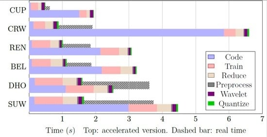
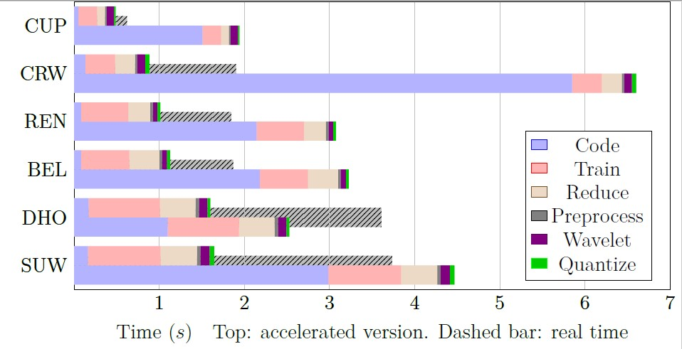
The speedup attained is shown in Figure 14. The average speedup obtained was 3.6, ranging from 1.6 for the DHOimage to 7.5 for the CRWimage.
6. Conclusions
JYPEC is a complex algorithm that demands high-performing hardware for a fast execution in real time. The most costly part is the tier 1 coder within JPEG2000, since code with erratic branching is very hard to optimize for traditional processors.
Very simple arithmetic and logic operations, however, make this part of the algorithm ideal for execution on a FPGA. A very fast architecture for the full tier 1 coder within JPEG2000 has been developed based on two main ideas:
- First, the bit plane coder concurrently processes bits in groups of four, greatly accelerating execution. A system of FIFOs and buffers ensure that a constant stream of CxD pairs reach the MQ-coder.
- Second, the coder itself is highly optimized in a pipelined fashion. Stalling of the pipeline, a problem previous designs had, is avoided by fusing together multiple updates when possible.
The presented design doubles the speed of any previous design on FPGA, coming close in performance to 0.18 m CMOS technology in single-core tests.
In the context of hyperspectral imaging, it brings complex lossy compression to real-time performance under the AVIRIS-ng sensor threshold (30–72 MS/s for a total of 491.52 Mb/s). This allows for very high data rates to be reduced for long-term storage on-the-fly, while keeping great quality for posterior analyses.
Author Contributions
D.B. designed the algorithm; C.G. and D.M. conceived and designed the experiments; D.B. performed the experiments; D.B., C.G. and D.M. analyzed the data; D.B., C.G. and D.M. wrote the paper. All authors have read and agreed to the published version of the manuscript.
Funding
This work has been supported by the by the Spanish MINECO projects TIN2013-40968-P and TIN2017-87237-P.
Acknowledgments
The authors would like to thank the anonymous reviewers. Their comments and suggestions greatly improved this paper.
Conflicts of Interest
The authors declare no conflict of interest.
References
- DataBase, I. A Database for Remote Sensing Indices. Available online: https://www.indexdatabase.de/db/s.php (accessed on 24 February 2020).
- eoPortal. Airborne Sensors. Available online: https://directory.eoportal.org/web/eoportal/airborne-sensors (accessed on 14 May 2020).
- Briottet, X.; Boucher, Y.; Dimmeler, A.; Malaplate, A.; Cini, A.; Diani, M.; Bekman, H.; Schwering, P.; Skauli, T.; Kasen, I.; et al. Military applications of hyperspectral imagery. Targets Backgrounds XII Charact. Represent. 2006, 6239, 62390B. [Google Scholar] [CrossRef] [Green Version]
- Tiwari, K.C.; Arora, M.K.; Singh, D. An assessment of independent component analysis for detection of military targets from hyperspectral images. Int. J. Appl. Earth Obs. Geoinf. 2011, 13, 730–740. [Google Scholar] [CrossRef]
- Slocum, K.; Surdu, J.; Sullivan, J.; Rudak, M.; Colvin, N.; Gates, C. Trafficability Analysis Engine. Cross Talk J. Def. Softw. Eng. 2003, 28–30. [Google Scholar]
- Murphy, R.J.; Monteiro, S.T.; Schneider, S. Evaluating classification techniques for mapping vertical geology using field-based hyperspectral sensors. IEEE Trans. Geosci. Remote Sens. 2012, 50, 3066–3080. [Google Scholar] [CrossRef]
- Kurz, T.H.; Buckley, S.J.; Howell, J.A.; Schneider, D. Geological outcrop modelling and interpretation using ground based hyperspectral and laser scanning data fusion. Int. Arch. Photogramm. Remote Sens. Spat. Inf. Sci. 2008, 37, 1229–1234. [Google Scholar]
- van der Meer, F.D.; van der Werff, H.M.; van Ruitenbeek, F.J.; Hecker, C.A.; Bakker, W.H.; Noomen, M.F.; van der Meijde, M.; Carranza, E.J.M.; de Smeth, J.B.; Woldai, T. Multi- and hyperspectral geologic remote sensing: A review. Int. J. Appl. Earth Obs. Geoinf. 2012, 14, 112–128. [Google Scholar] [CrossRef]
- Thenkabail, P.; Lyon, J.; Huete, A. (Eds.) Hyperspectral Indices and Image Classifications for Agriculture and Vegetation. 2018. Available online: https://www.taylorfrancis.com/books/9781315159331/chapters/10.1201/9781315159331-1 (accessed on 16 July 2020).
- Lu, J.; Yang, T.; Su, X.; Qi, H.; Yao, X.; Cheng, T.; Zhu, Y.; Cao, W.; Tian, Y. Monitoring leaf potassium content using hyperspectral vegetation indices in rice leaves. Precis. Agric. 2019, 21, 324–348. [Google Scholar] [CrossRef]
- eoPortal. EnMAP (Environmental Monitoring and Analysis Program). Available online: https://directory.eoportal.org/web/eoportal/satellite-missions/e/enmap (accessed on 5 August 2020).
- CCSDS. Low-Complexity Lossless and Near-Lossless Multispectral and Hyperspectral Image Compression. Available online: https://public.ccsds.org/Pubs/123x0b2c1.pdf (accessed on 8 August 2020).
- Motta, G.; Rizzo, F.; Storer, J.A. Hyperspectral Data Compression; Springer Science & Business Media: Berlin, Germany, 2006; p. 417. [Google Scholar]
- Ryan, M.J.; Arnold, J.F. The lossless compression of aviris images by vector quantization. IEEE Trans. Geosci. Remote Sens. 1997, 35, 546–550. [Google Scholar] [CrossRef]
- Abrardo, A.; Barni, M.; Magli, E. Low-complexity predictive lossy compression of hyperspectral and ultraspectral images. In Proceedings of the 2011 IEEE International Conference on Acoustics, Speech and Signal Processing (ICASSP), Prague, Czech Republic, 22–27 May 2011; pp. 797–800. [Google Scholar] [CrossRef]
- Fowler, J.; Rucker, J. 3D wavelet-based compression of hyperspectral imagery. In Hyperspectral Data Exploitation: Theory and Applications; John Wiley & Sons: Hoboken, NJ, USA, 2007; pp. 379–407. [Google Scholar]
- Christophe, E.; Mailhes, C.; Duhamel, P. Hyperspectral image compression: Adapting SPIHT and EZW to anisotropic 3-D wavelet coding. IEEE Trans. Image Process. 2008, 17, 2334–2346. [Google Scholar] [CrossRef] [Green Version]
- Huang, B. Satellite Data Compression; Springer Science & Business Media: Berlin, Germany, 2011. [Google Scholar]
- Du, Q.; Fowler, J.E. Hyperspectral image compression using JPEG2000 and principal component analysis. IEEE Geosci. Remote Sens. Lett. 2007, 4, 201–205. [Google Scholar] [CrossRef]
- Báscones, D.; González, C.; Mozos, D. Hyperspectral Image Compression Using Vector Quantization, PCA and JPEG2000. Remote Sens. 2018, 10, 907. [Google Scholar] [CrossRef] [Green Version]
- Taubman, D.; Marcellin, M. JPEG2000 Image Compression Fundamentals, Standards and Practice; Springer Science & Business Media: Berlin, Germay, 2012; Volume 642, p. 773. [Google Scholar] [CrossRef]
- Skodras, A.; Christopoulos, C.; Ebrahimi, T. The JPEG 2000 Still Image Compression Standard. IEEE Signal Process. Mag. 2001, 18, 36–58. [Google Scholar] [CrossRef]
- Wallace, G.K. The JPEG still picture compression standard. IEEE Trans. Consum. Electron. 1992. [Google Scholar] [CrossRef]
- Gangadhar, M.; Bhatia, D. FPGA based EBCOT architecture for JPEG 2000. Microprocess. Microsyst. 2003, 29, 363–373. [Google Scholar] [CrossRef]
- Lian, C.J.; Chen, K.F.; Chen, H.H.; Chen, L.G. Analysis and architecture design of block-coding engine for EBCOT in JPEG 2000. IEEE Trans. Circuits Syst. Video Technol. 2003, 13, 219–230. [Google Scholar] [CrossRef]
- Dyer, M.; Taubman, D.; Nooshabadi, S.; Gupta, A.K. Concurrency techniques for arithmetic coding in JPEG2000. IEEE Trans. Circuits Syst. I Regul. Pap. 2006, 53, 1203–1213. [Google Scholar] [CrossRef]
- Gupta, A.K.; Taubman, D.S.; Nooshabadi, S. High speed VLSI architecture for bit plane encoder of JPEG 2000. IEEE Midwest Sympos. Circuits Syst. 2004, 2, 233–236. [Google Scholar] [CrossRef]
- Kai, L.; Chengke, W.; Yunsong, L. A high-performance VLSI arquitecture of EBCOT block coding in JPEG2000. J. Electron. 2006, 23, 1–5. [Google Scholar]
- Sarawadekar, K.; Banerjee, S. Low-cost, high-performance VLSI design of an MQ coder for JPEG 2000. In Proceedings of the IEEE 10th International Conference on Signal Processing Proceedings, Beijing, China, 24–28 October 2010; Number D. pp. 397–400. [Google Scholar]
- Saidani, T.; Atri, M.; Tourki, R. Implementation of JPEG 2000 MQ-coder. In Proceedings of the 2008 3rd International Conference on Design and Technology of Integrated Systems in Nanoscale Era, Tozeur, Tunisia, 25–27 March 2008; pp. 1–4. [Google Scholar] [CrossRef]
- Sarawadekar, K.; Banerjee, S. VLSI design of memory-efficient, high-speed baseline MQ coder for JPEG 2000. Integr. VLSI J. 2012, 45, 1–8. [Google Scholar] [CrossRef]
- Liu, K.; Zhou, Y.; Li, Y.S.; Ma, J.F.; Song Li, Y.; Ma, J.F. A high performance MQ encoder architecture in JPEG2000. Integr. VLSI J. 2010, 43, 305–317. [Google Scholar] [CrossRef]
- Sulaiman, N.; Obaid, Z.A.; Marhaban, M.H.; Hamidon, M.N. Design and Implementation of FPGA-Based Systems—A Review. Aust. J. Basic Appl. Sci. 2009, 3, 3575–3596. [Google Scholar]
- Trimberger, S.M. Three ages of FPGAs: A retrospective on the first thirty years of FPGA technology. Proc. IEEE 2015, 103, 318–331. [Google Scholar] [CrossRef]
- Xilinx. Space-Grade Virtex-5QV FPGA. Available online: www.xilinx.com/products/silicon-devices/fpga/virtex-5qv.html (accessed on 8 August 2020).
- Báscones, D.; González, C.; Mozos, D. Parallel Implementation of the CCSDS 1.2.3 Standard for Hyperspectral Lossless Compression. Remote Sens. 2017, 9, 973. [Google Scholar] [CrossRef] [Green Version]
- Báscones, D.; Gonzalez, C.; Mozos, D. FPGA Implementation of the CCSDS 1.2.3 Standard for Real-Time Hyperspectral Lossless Compression. IEEE J. Sel. Top. Appl. Earth Obs. Remote Sens. 2017, 11, 1158–1165. [Google Scholar] [CrossRef]
- Bascones, D.; Gonzalez, C.; Mozos, D. An Extremely Pipelined FPGA Implementation of a Lossy Hyperspectral Image Compression Algorithm. IEEE Trans. Geosci. Remote Sens. 2020, 1–13. [Google Scholar] [CrossRef]
- Báscones, D. Implementación Sobre FPGA de un Algoritmo de Compresión de Imágenes Hiperespectrales Basado en JPEG2000. Ph.D. Thesis, Universidad Complutense de Madrid, Madrid, Spain, 2018. [Google Scholar]
- Higgins, G.; Faul, S.; McEvoy, R.P.; McGinley, B.; Glavin, M.; Marnane, W.P.; Jones, E. EEG compression using JPEG2000 how much loss is too much? In Proceedings of the 2010 Annual International Conference of the IEEE Engineering in Medicine and Biology Society, EMBC’10, Buenos Aires, Argentina, 31 August–4 September 2010; pp. 614–617. [Google Scholar] [CrossRef]
- Marpe, D.; George, V.; Cycon, H.L.; Barthel, K.U. Performance evaluation of Motion-JPEG2000 in comparison with H.264/AVC operated in pure intra coding mode. SPIE Proc. 2003, 5266, 129–137. [Google Scholar] [CrossRef] [Green Version]
- Van Fleet, P.J. Discrete Wavelet Transformations: An Elementary Approach with Applications; John Wiley & Sons: Hoboken, NJ, USA, 2011. [Google Scholar] [CrossRef]
- Makandar, A.; Halalli, B. Image Enhancement Techniques using Highpass and Lowpass Filters. Int. J. Comput. Appl. 2015, 109, 12–15. [Google Scholar] [CrossRef]
- Taubman, D. High performance scalable image compression with EBCOT. IEEE Trans. Image Process. 2000, 9, 1158–1170. [Google Scholar] [CrossRef]
- Andra, K.; Acharya, T.; Chakrabarti, C. Efficient VLSI implementation of bit plane coder of JPEG2000. Appl. Digit. Image Process. Xxiv 2001, 4472, 246–257. [Google Scholar] [CrossRef]
- Li, Y.; Bayoumi, M.A. A three level parallel high speed low power architecture for EBCOT of JPEG 2000. IEEE Trans. Circuits Syst. Video Technol. 2006, 16, 1153–1163. [Google Scholar] [CrossRef]
- Jayavathi, S.D.; Shenbagavalli, A. FPGA Implementation of MQ Coder in JPEG 2000 Standard—A Review. 2016, 28, 76–83. Int. J. Innov. Sci. Res. 2016, 28, 76–83. [Google Scholar]
- Rhu, M.; Park, I.C. Optimization of arithmetic coding for JPEG2000. IEEE Trans. Circuits Syst. Video Technol. 2010, 20, 446–451. [Google Scholar] [CrossRef]
- Ahmadvand, M.; Ezhdehakosh, A. A New Pipelined Architecture for JPEG2000. World Congress Eng. Comput. Sci. 2012, 2, 24–26. [Google Scholar]
- Mei, K.; Zheng, N.; Huang, C.; Liu, Y.; Zeng, Q. VLSI design of a high-speed and area-efficient JPEG2000 encoder. IEEE Trans. Circuits Syst. Video Technol. 2007, 17, 1065–1078. [Google Scholar] [CrossRef]
- Chang, Y.W.; Fang, H.C.; Chen, L.G. High Performance Two-Symbol Arithmetic Encoder in JPEG 2000. 2000, pp. 4–7. Available online: https://video.ee.ntu.edu.tw/publication/paper/[C][2004][ICCE][Yu-Wei.Chang][1].pdf (accessed on 8 August 2020).
- Kumar, N.R.; Xiang, W.; Wang, Y. An FPGA-based fast two-symbol processing architecture for JPEG 2000 arithmetic coding. In Proceedings of the 2010 IEEE International Conference on Acoustics, Speech and Signal Processing, Dallas, TX, USA, 14–19 March 2010; pp. 1282–1285. [Google Scholar] [CrossRef] [Green Version]
- Sarawadekar, K.; Banerjee, S. An Efficient Pass-Parallel Architecture for Embedded Block Coder in JPEG 2000. IEEE Trans. Circuits Syst. 2011, 21, 825–836. [Google Scholar] [CrossRef]
- Kumar, N.R.; Xiang, W.; Wang, Y. Two-symbol FPGA architecture for fast arithmetic encoding in JPEG 2000. J. Signal Process. Syst. 2012, 69, 213–224. [Google Scholar] [CrossRef]
- Spectir. Free Data Samples. Available online: https://www.spectir.com/free-data-samples/ (accessed on 5 August 2020).
- CCSDS. Collaborative Work Environment. Available online: https://cwe.ccsds.org/sls/default.aspx (accessed on 5 August 2020).
- Báscones, D. Jypec. Available online: github.com/Daniel-BG/Jypec (accessed on 17 January 2018).
- Báscones, D. Vypec. Available online: github.com/Daniel-BG/Vypec (accessed on 25 January 2018).
Figure 1.
Diagram of the full JYPEC algorithm.

Figure 2.
Diagram of the full JPEG2000 algorithm. In green, steps that deal with the whole image at once. In blue, steps that deal with small blocks of the image.
Figure 2.
Diagram of the full JPEG2000 algorithm. In green, steps that deal with the whole image at once. In blue, steps that deal with small blocks of the image.

Figure 3.
Bit plane coder. The zig-zag pattern can be seen (four rows visited column by column). This is repeated three times (three passes) until all bits from a plane have been visited. The sign bit plane (red) is coded separately.
Figure 3.
Bit plane coder. The zig-zag pattern can be seen (four rows visited column by column). This is repeated three times (three passes) until all bits from a plane have been visited. The sign bit plane (red) is coded separately.

Figure 4.
Timing breakdown when compressing a set of hyperspectral images with JYPEC. Steps are sorted by time. While training takes a fair bit of time, coding is clearly the bottleneck of the process.
Figure 4.
Timing breakdown when compressing a set of hyperspectral images with JYPEC. Steps are sorted by time. While training takes a fair bit of time, coding is clearly the bottleneck of the process.

Figure 5.
Tier 1 coder architecture.

Figure 6.
BPC structure. indicates sign bits for the current strip. m indicates magnitude bits for the current strip. is the coded flag for the strip, indicating whether each bit is coded. is yet another flag indicating, for each bit, whether it is being refined for the first time. s is the significance status for the neighborhood of the strip. are flags indicating the current pass (significance, cleanup, refinement). Flags are updated for the next pass and output to memory. The contexts for each pass exit the context generation () modules for all three passes () along with the xor bit for the sign. This ends up being output as a vector of triplets , containing the context–data (CxD) pairs as well as a valid bit.

Figure 7.
Significance predictor module. It cascades the possible significance conversion of all bits in the strip by using a small critical path, instead of waiting for the cascade of modules. The significances s, magnitude bits m, and sign bits are used to produce the new significance . It is output along with a flag , indicating if it is a newly acquired significance this cycle.

Figure 8.
BPC architecture. The BPC core generates up to 10 CxD pairs per cycle, which are then serialized before sending them to the CxD FIFO.
Figure 8.
BPC architecture. The BPC core generates up to 10 CxD pairs per cycle, which are then serialized before sending them to the CxD FIFO.

Figure 9.
MQ-coder architecture. The interval updates are fused when possible, having less bound updates which could stall the pipeline.
Figure 9.
MQ-coder architecture. The interval updates are fused when possible, having less bound updates which could stall the pipeline.

Figure 10.
MQ-coder first and second stages. The context and bit from the BPC are input, and a probability, shift, and hit (correct prediction or not) are output.
Figure 10.
MQ-coder first and second stages. The context and bit from the BPC are input, and a probability, shift, and hit (correct prediction or not) are output.

Figure 11.
MQ-coder last stage. It interfaces with two FIFOs, reading updates from the previous stage and making sure space is available at the output to send bytes out.
Figure 11.
MQ-coder last stage. It interfaces with two FIFOs, reading updates from the previous stage and making sure space is available at the output to send bytes out.

Figure 12.
Detailed pipeline of the tier 1 coder. In dotted orange, the separation between stages. Each FIFO introduces two stages (read/write).
Figure 12.
Detailed pipeline of the tier 1 coder. In dotted orange, the separation between stages. Each FIFO introduces two stages (read/write).

Figure 13.
Small cutouts of the images from Table 3. In reading order: CUP, SUW, DHO, BEL, REN, CRW.
Figure 13.
Small cutouts of the images from Table 3. In reading order: CUP, SUW, DHO, BEL, REN, CRW.

Figure 14.
Speedup when using an FPGA as an accelerator. For each image, the top bars indicate the sped-up version, and the bottom bars are the non-sped-up one. A dashed bar indicates the real-time threshold, which without acceleration was only met by the DHO image.
Figure 14.
Speedup when using an FPGA as an accelerator. For each image, the top bars indicate the sped-up version, and the bottom bars are the non-sped-up one. A dashed bar indicates the real-time threshold, which without acceleration was only met by the DHO image.


Table 1.
Frequency and occupancy for the different modules that make the full tier 1 coder. Results are for the Virtex-7 XC7VX690T board with a depth of 32 set for all queues.
Table 1.
Frequency and occupancy for the different modules that make the full tier 1 coder. Results are for the Virtex-7 XC7VX690T board with a depth of 32 set for all queues.
| Module | Frequency (MHz) | Slices | BRAM |
|---|---|---|---|
| Tier 1 coder | 255 | 2708 | 4 |
| BPC-core | 248 | 731 | 2 |
| BPC-serial | 390 | 142 | 0 |
| MQ | 321 | 1778 | 0 |
| MQ-I/II | 322 | 1326 | 0 |
| MQ-III | 535 | 47 | 0 |
| MQ-IV | 331 | 231 | 0 |
| FIFOs | 927 | 57 | 2 |
Table 2.
Comparison with other implementations.
| Coder | Ref. | Technology | Frequency | Speed | Slices | BRAM/b |
|---|---|---|---|---|---|---|
| BPC | [27] | APEX20KE FPGA | 51.7 MHz | 73.44 Mb/s | 956 | n/a ** |
| [28] | XCV600e-6BG432 | 52.0 MHz | 94.4 Mb/s | n/a | n/a ** | |
| [50] | Altera EP20K600EFC672–3 | 100.0 MHz | 40.5 Mb/s | 1850 | 0 ** | |
| This | Virtex-7 FPGA | 247.8 MHz | 368.8 Mb/s | 731 | 2 | |
| MQ | [51] | 0.35 m | 90.0 MHz | 180.0 MCxD/s | n/a | n/a |
| [46] | 0.35 m | 150.0 MHz | 300.0 MCxD/s | n/a | n/a | |
| [26] | Stratix | 48.8 MHz | 97.7 MCxD/s | 1596 | 8192 b | |
| [26] | 0.18 m | 211.8 MHz | 423.7 MCxD/s | n/a | n/a | |
| [50] | Altera EP20K600EFC672–3 | 26.3 MHz | 52.6 MCxD/s | 1811 | n/a | |
| [29] | Stratix FPGA | 153.0 MHz | 137.7 MCxD/s | 279 | 1344 b | |
| [48] | 0.18 m | 413.0 MHz | 413.0 MCxD/s | n/a | n/a | |
| [52] | Stratix FPGA | 106.2 MHz | 212.4 MCxD/s | 1267 | 0 | |
| [32] | XC4VLX80 FPGA | 48.3 MHz | 96.6 MCxD/s | 6974 | 1509 b | |
| [32] | 0.18 m | 220.0 MHz | 440.0 MCxD/s | n/a | n/a | |
| [53] | Stratix EP1S10B672C6 | 136.9 MHz | 136.9 MCxD/s | 695 | 3301 b | |
| [31] | Stratix FPGA | 146.0 MHz | 146.0 MCxD/s | 824 | 428 b | |
| [49] | 0.18 m | 208.0 MHz | 192.8 MCxD/s | n/a | n/a | |
| [54] | Stratix II FPGA | 106.2 MHz | 212.4 MCxD/s | 1267 | 1321 b | |
| This | Virtex-7 FPGA | 321.5 MHz | 321.5 MCxD/s | 1778 | 0 | |
| Tier 1 | [25] | 0.35 m | 50.0 MHz | 36.5 Mb/s | n/a | n/a |
| [24] | Virtex II XC2V1000 | 50.0 MHz | 91.2 Mb/s | 4420 | 3120 b ** | |
| [30] | Virtex II Pro FG 456 | 112.0 MHz | 181.6 Mb/s * | 2504 | 28 | |
| This | Virtex-7 FPGA | 255.3 MHz | 380.0 Mb/s | 2708 | 4 |
* Although not specified, the architecture is similar to the one presented here so a similar relationship between frequency and speed was expected. ** Requires external memory for data and/or internal variables.
Table 3.
Images used for testing.
| Image | Bit Depth | Description | |||
|---|---|---|---|---|---|
| CUP [56] | 350 | 350 | 188 | 16 | Cuprite valley in Nevada |
| SUW [55] | 320 | 1200 | 360 | 16 | Lower Suwannee natural reserve |
| DHO [55] | 320 | 1260 | 360 | 16 | Deepwater Horizon oil spill |
| BEL [55] | 320 | 600 | 360 | 16 | Crop fields in Belstville |
| REN [55] | 320 | 600 | 356 | 16 | Urban and rural mixed area |
| CRW [56] | 614 | 512 | 224 | 16 | Cuprite valley full image |
© 2020 by the authors. Licensee MDPI, Basel, Switzerland. This article is an open access article distributed under the terms and conditions of the Creative Commons Attribution (CC BY) license (http://creativecommons.org/licenses/by/4.0/).
Share and Cite
MDPI and ACS Style
Báscones, D.; González, C.; Mozos, D. An FPGA Accelerator for Real-Time Lossy Compression of Hyperspectral Images. Remote Sens. 2020, 12, 2563. https://0-doi-org.brum.beds.ac.uk/10.3390/rs12162563
AMA Style
Báscones D, González C, Mozos D. An FPGA Accelerator for Real-Time Lossy Compression of Hyperspectral Images. Remote Sensing. 2020; 12(16):2563. https://0-doi-org.brum.beds.ac.uk/10.3390/rs12162563
Chicago/Turabian StyleBáscones, Daniel, Carlos González, and Daniel Mozos. 2020. "An FPGA Accelerator for Real-Time Lossy Compression of Hyperspectral Images" Remote Sensing 12, no. 16: 2563. https://0-doi-org.brum.beds.ac.uk/10.3390/rs12162563
Note that from the first issue of 2016, this journal uses article numbers instead of page numbers. See further details here.