Toward Mapping Dietary Fibers in Northern Ecosystems Using Hyperspectral and Multispectral Data


1
Department of Natural Resources and Society, University of Idaho, Moscow, ID 83844, USA
2
McCall Outdoor Science School, University of Idaho, McCall, ID 83638, USA
3
U.S. Department of Agriculture, Forest Service, Rocky Mountain Research Station, Moscow, ID 83843, USA
*
Author to whom correspondence should be addressed.
†
PhD Candidate University of Idaho.
Remote Sens. 2020, 12(16), 2579; https://0-doi-org.brum.beds.ac.uk/10.3390/rs12162579
Submission received: 22 July 2020
/
Revised: 6 August 2020
/
Accepted: 10 August 2020
/
Published: 11 August 2020
(This article belongs to the Special Issue Spectroscopic Analysis of Plants and Vegetation)
Abstract
:Shrub proliferation across the Arctic from climate warming is expanding herbivore habitat but may also alter forage quality. Dietary fibers—an important component of forage quality—influence shrub palatability, and changes in dietary fiber concentrations may have broad ecological implications. While airborne hyperspectral instruments may effectively estimate dietary fibers, such data captures a limited portion of landscapes. Satellite data such as the multispectral WorldView-3 (WV-3) instrument may enable dietary fiber estimation to be extrapolated across larger areas. We assessed how variation in dietary fibers of Salix alaxensis (Andersson), a palatable northern shrub, could be estimated using hyperspectral and multispectral WV-3 spectral vegetation indices (SVIs) in a greenhouse setting, and whether including structural information (i.e., leaf area) would improve predictions. We collected canopy-level hyperspectral reflectance readings, which we convolved to the band equivalent reflectance of WV-3. We calculated every possible SVI combination using hyperspectral and convolved WV-3 bands. We identified the best performing SVIs for both sensors using the coefficient of determination (adjusted R2) and the root mean square error (RMSE) using simple linear regression. Next, we assessed the importance of plant structure by adding shade leaf area, sun leaf area, and total leaf area to models individually. We evaluated model fits using Akaike’s information criterion for small sample sizes and conducted leave-one-out cross validation. We compared cross validation slopes and predictive power (Spearman rank coefficients ) between models. Hyperspectral SVIs (R2 = 0.48–0.68; RMSE = 0.04–0.91%) outperformed WV-3 SVIs (R2 = 0.13–0.35; RMSE = 0.05–1.18%) for estimating dietary fibers, suggesting hyperspectral remote sensing is best suited for estimating dietary fibers in a palatable northern shrub. Three dietary fibers showed improved predictive power when leaf area metrics were included (cross validation = +2–8%), suggesting plant structure and the light environment may augment our ability to estimate some dietary fibers in northern landscapes. Monitoring dietary fibers in northern ecosystems may benefit from upcoming hyperspectral satellites such as the environmental mapping and analysis program (EnMAP).
1. Introduction
Accelerated warming in high latitude regions (i.e., ≥60°N) has led to warmer, wetter, and more variable environments [1,2]. One consequence of accelerated warming in these regions is the increased abundance and geographic extent of shrubs [3,4]. Some herbivores are expanding their ranges to exploit these increased food resources [5,6] and also regulate vegetation proliferation through browsing [7,8] and soil fertilization [9,10]. The effect of herbivores on shrubs is influenced by herbivore density, foraging intensity, and the palatability of shrubs [8,11]. Shrub palatability may be influenced by increased temperatures from environmental change, which has broad ecosystem implications such as alterations to nutrient cycling [12,13].
Characterizing palatability—or forage quality—for herbivores is complex. Nitrogen content, foliar defense compounds, and dietary fibers must all be considered when quantifying forage quality [14]. Dietary fibers encompass the structural components of plant cell walls, primarily hemicellulose (HMC), cellulose (CLL), and lignin, but can also be quantified in the laboratory for technical fiber fractions: neutral detergent fiber (NDF), acid detergent fiber (ADF), acid detergent lignin (ADL), and acid insoluble ash (AIA, or silica) [15]. Higher fiber levels often increase handling time (i.e., cropping, chewing, and digesting) [16], and therefore reduce plant palatability. However, CLL and HMC can provide substantial energy for ruminants (up to 80%) [17].
Quantifying and mapping forage resources for herbivores are critical to effective management. Remote sensing provides a means of characterizing and monitoring forage quality across the landscape. Optical remote sensing approaches use reflected light from the ultraviolet (10–380 nm), visible (400–700 nm), near infrared (NIR; 701–1399 nm), and shortwave infrared (SWIR; 1400–2500 nm) regions to estimate plant dynamics. Reflected light from vegetation is influenced by functional group, plant water content, plant structural components, and foliar chemistry [18]. Spectral vegetation indices (SVIs) calculated from spectral data are generated using simple algebraic formulas that enhance a target’s spectral signal, and are commonly used to characterize vegetation vigor, growth, and foliar chemistry [18]. For example, the normalized difference vegetation index (NDVI) [19] is often used to predict habitat quality and takes the mathematical form of (NIR-Red)/(NIR + Red). However, NDVI often has mixed results when used to track forage resources [20,21]. This limitation may be linked to the spectral resolution of broad band imagery that is not able to detect small absorption features associated with foliar biochemical traits.
Hyperspectral instruments sample the electromagnetic spectrum at narrow, contiguous wavelength ranges, which results in hundreds of sampled wavelengths. Generally, wavelengths greater than 700 nm show measurable absorption and scattering features that track dietary fibers such as CLL and lignin [22], particularly in the SWIR region [23,24]. HMC and CLL have been accurately estimated using hyperspectral instruments in a variety of ecosystems from grasslands [25,26] to complex forests [27]. Similarly, NDF and ADF have also been accurately estimated via hyperspectral remote sensing in semiarid rangelands [28,29].
Although SVIs calculated from remotely sensed spectral data have demonstrated their utility in detecting various vegetation characteristics, they also show considerable sensitivity to plant structure such as leaf area index (LAI) [30,31]. Canopy structural variation strongly influences spectral reflectance characteristics by creating a more complex three-dimensional environment for photons to interact [32,33,34]. Thus, plants with higher LAI have a more complex canopy and therefore amplify biochemical signals through scattering in NIR and to a lesser extent the SWIR regions [32].
Complex canopy architecture also influences the light environment within the canopy, impacting photosynthesis, growth, and nutrient quality for herbivores. For instance, diamond leaf willow (Salix planifolia pulchra) in Alaska demonstrated varying levels of NDF and ADF between sun and shaded leaves and a decrease in digestibility for willows growing in the sun [35]. Similarly, palatable shrubs growing in shaded conditions had significantly reduced levels of HMC but increased levels of CLL than sunlit shrubs of the same species [36]. Thus, incorporating plant structural metrics and the distinction between sun and shaded leaves into models designed to predict dietary fibers may improve model performance.
Although hyperspectral instruments can resolve fine-scale foliar chemistry, few hyperspectral satellites exist, and airborne data captures only a small portion of the landscape used by wildlife. However, the high-spatial resolution (<5 m pixels) of multispectral imagery from WorldView satellites may enable fine-scale forage quality estimation, though the broadband imagery (bandwidth 40–70 nm) lacks the spectral resolution of hyperspectral data. WorldView-2 (WV-2) and WorldView-3 (WV-3) sensors have shown promise in estimating foliar nitrogen content in rangelands [37,38], crop residues in agricultural settings [39], and digestible protein in eucalyptus forests [40]. WorldView satellites also demonstrate utility in mapping percent vegetation cover [41] and plant functional type [42] in Arctic regions. WV-3 includes eight SWIR bands, yet to our knowledge no study has yet assessed the utility of the WV-3 satellite to map dietary fibers in high latitude settings.
Evaluating sensor performance in measuring dietary fibers in high latitude regions is increasingly important because of the effect of warming on palatable shrubs. Therefore, our overarching objective was to assess whether variation in six dietary fibers could be estimated by using multispectral bands from the WV-3 satellite, relative to hyperspectral data. To control for variations in environmental conditions, we conducted a greenhouse experiment with a highly palatable shrub common in Boreal and Arctic ecosystems, feltleaf willow (Salix alaxensis (Andersson)). We collected hyperspectral measures at two time intervals and identified hyperspectral SVIs suitable to remotely sense two functional fibers (HMC and CLL) and four technical fibers (NDF, ADF, ADL, and AIA) collectively called ‘dietary fibers’ hereafter. Second, we assessed the value of incorporating shrub structure and the light environment into our models using leaf area (cm2) from sun and shaded leaves from each sample. Finally, we evaluated the suitability of the WV-3 satellite to monitor dietary fibers across the landscape using the band equivalent reflectance (BER) for each band by convolving our hyperspectral measures.
We hypothesized that the best SVIs would contain wavelengths >700 nm [22] and that the SWIR region [23,24] would be best suited for tracking dietary fibers. We also predicted the BER of WV-3 would be able to estimate dietary fibers moderately well because of its eight SWIR bands. Further, we hypothesized that accounting for leaf area would enhance our models because higher levels of LAI have been shown to amplify biochemical signals in the NIR and SWIR regions [32]. Finally, we hypothesized that partitioning leaf area into sun and shaded fractions would contribute meaningful differences in model performance because dietary fiber concentrations vary between sunlit and shaded canopies [35,36].
2. Materials and Methods
2.1. Greenhouse Procedures
On 13 June 2018, we collected 52 willow (Salix alaxensis (Andersson)) cuttings near Coldfoot, AK (67.2524°N, −150.1772°W). We stored cuttings in a chilled cooler for transit, and cuttings were wrapped in moist paper towels and provided water through a plastic reservoir attached to each cut stem. Twenty-four hours later, we processed field cuttings by clipping small wooded stems and current year green stems. We dipped these new clippings in a solution of indol-3-butyric acid (0.2%) rooting hormone and planted them in trays containing a water-saturated, peat moss, and vermiculite (1:1 by volume) media. Trays were placed inside a misting chamber outfitted with a root zone heat mat set to 17 °C.
Available nutrients for high latitude plants are expected to increase as temperatures rise, which in turn increases shrub biomass [3] and therefore dietary fibers. Thus, we simulated a broad range of possible nitrogen (N) concentration scenarios that may occur as the rate of nutrient cycling increases (Appendix A). Four weeks after the second clipping, when cuttings had generated new roots, we randomly stratified willow cuttings (n = 105) into six groups along a gradient of N-fertilizer treatments: native; +5; +10; +20; +50; and +100 kg N ha−1. After treatment groups were assigned, we transferred rooted-cuttings into larger, 2.3 L Treepot containers (Stuewe & Sons, Inc. Tangent, OR, USA) containing artificial media (peat moss, vermiculite, and perlite; 2:1:1 by volume) and the total amount of N required for the study. N, phosphorus (P), potassium, (K), and micronutrients were delivered via controlled-release fertilizer (Osmocote Plus, 5–6 month, NPK: 15-9-12). Water was provided via subirrigation and timing was determined gravimetrically [43]. Feltleaf willows grow primarily in riparian areas so gravimetric irrigation targets were set to 70–80% of saturation.
Our samples experienced a large amount of attrition (43%) related to disease (willow rust, Melampsora spp.) and pests (aphid outbreak) within the first month of the experiment. Thus, we opted to put the remaining samples into dormancy for the winter and to restart the experiment in March 2019. On 11 January 2019, willows were wrapped in moist paper towels, stored in paper bags inside of a freezer set to −2.2 °C. After 8 weeks in dormancy, willows were thawed at 15.6–18.3 °C for three days. Once willows were thawed, we replanted them using the same procedures outlined previously. Sixty plants were viable from the first round of the experiment. From March through June 2019, greenhouse temperatures averaged 23.6/17.4 °C (day/night), relative humidity averaged 41.7/62.0% (day/night), and photosynthetically active radiation (PAR) peaked at 1190 μmol during the experimental period (March–June 2019).
For each round of sampling, we randomly selected 12 willows for harvest. Although we had planned to conduct a third and fourth round of sampling, our plants again experienced a pest outbreak. Therefore, we only sampled two rounds and obtained 24 samples total—one and two months after planting, 6 May and 2 June, respectively.
2.2. Hyperspectral, Leaf Area, and Destructive Vegetation Collection
We collected hyperspectral reflectance readings and associated destructive-vegetation samples from each replicate. We collected canopy spectra using a FieldSpec Pro Full Range Spectroradiometer (Malvern Panalytical Ltd., Malvern, UK). This instrument has a spectral range of 350–2500 nm, with a full-width half-max of 3 nm in the visible and near infrared regions (350–1050 nm), and 10–12 nm in both short-wave infrared regions (900–1850 nm and 1700–2500 nm). Prior to sampling of each plant, dark current and white reference measures were taken using Spectralon panel (Labsphere, Inc., North Sutton, NH, USA).
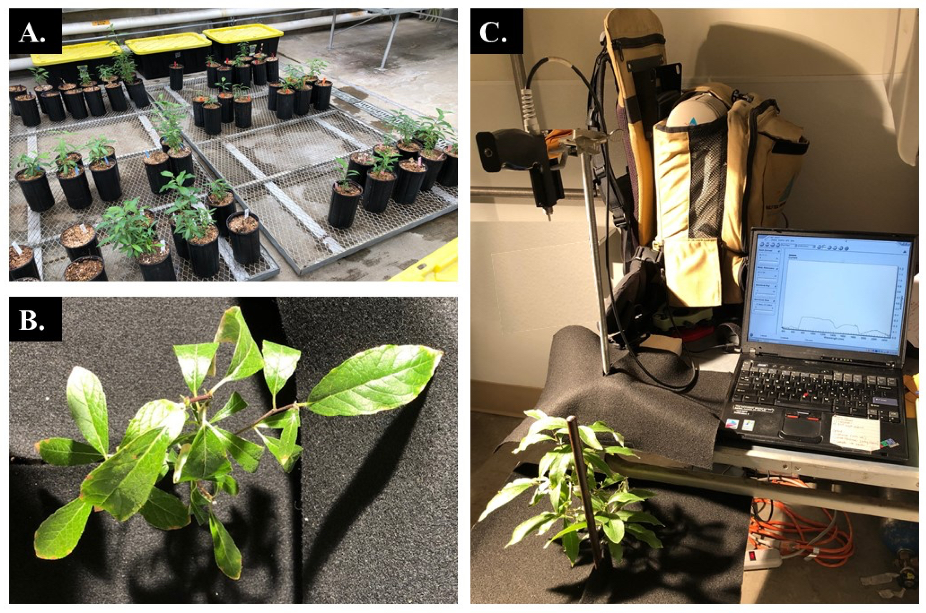
The fiber optic probe of the instrument (with a 25° field of view) was mounted 50 cm above the highest point of each plant (Figure 1C). Each sampled plant was illuminated with a full spectrum lamp (1000 W) mounted at a 60° zenith angle 1.4 m above the ground. To minimize confounding background effects on spectral measurements, a spectrally flat black-foam material was cut and placed around the lowest point of the stem of each willow (Figure 1B). Four spectral measurements were taken per willow, and the willow was rotated 90° each round of sampling. We calculated the mean of these four spectral measurements for analysis.
Immediately after collecting canopy spectra, leaves were harvested, separated into ‘shade’ and ‘sun’ categories based on a visual assessment of their position in the canopy and scanned using a portable scanner. We included a reference target of a known area in each scan that enabled us to calculate one-sided leaf area (cm2) in Image J [44] following methods outlined in [45]. After scanning, leaves were oven dried for 48 h at 30–40 °C. Dried samples were ground and analyzed by the Washington State University Habitat Lab for NDF, ADF, ADL, and AIA using the sequential fiber analysis [15]. We estimated HMC content by subtracting ADF from NDF, and CLL content by subtracting ADL from ADF.
2.3. Statistical Analyses
We used R statistical software version 3.6.2 [46] for all statistical assessments. We tested for differences in dietary fibers between sample periods using Welch’s two sample t-test [47] and differences between dietary fibers and N fertilization treatments using a one way analysis of variance (ANOVA) and Tukey’s range test [48] as a post hoc follow up to determine pairwise differences between fertilizer treatments.
We assessed every possible spectral band combination using simple ratio SVIs (Band A/Band B) and also normalized differenced SVIs ((Band A − Band B)/(Band A + Band B)) to track dietary fibers using simple linear models. The best performing SVIs for each dietary fiber were identified using adjusted R2 values and the root mean square error (RMSE). After identifying the best performing SVIs, we assessed the importance of plant structure by adding shade leaf area, sun leaf area, and total leaf area to linear models individually. We evaluated model fit between model variants using Akaike’s information criterion for small sample sizes (AICc) [49,50] from the ‘MuMIn’ package [51]. We also conducted leave-one-out cross validation (LOOCV) by excluding one willow from the data set sequentially and testing the predictive power of the remaining willows against the excluded one. We compare the resultant slopes and predictive power using Spearman rank coefficients () between models.
2.4. Band Equivalent Reflectance
The BER provides an assessment of potential sensor performance [52]. To assess the ability of identified SVIs to scale to the landscape level, SVIs identified from canopy-level hyperspectral data were convolved to WV-3 satellite bands using their BER [53]. The spectral response functions of WV-3 were obtained directly from Maxar Technologies (Westminster, CO, USA). The BER data for WV-3 were then used to recompute SVIs. As with the hyperspectral SVIs, we assessed whether adding shade leaf area, sun leaf area, and total leaf area improved our models following the same analytical steps detailed in Section 2.3. Since we hypothesized that incorporating leaf area into models would improve model performance, we also investigated the relationships between total leaf area and NDVI, which has been shown to have a strong nonlinear relationship with LAI in high latitude regions [54]. Finally, we substituted NDVI for total leaf area in our WV-3 BER models to evaluate the possibility of representing plant structure using only SVIs.
3. Results
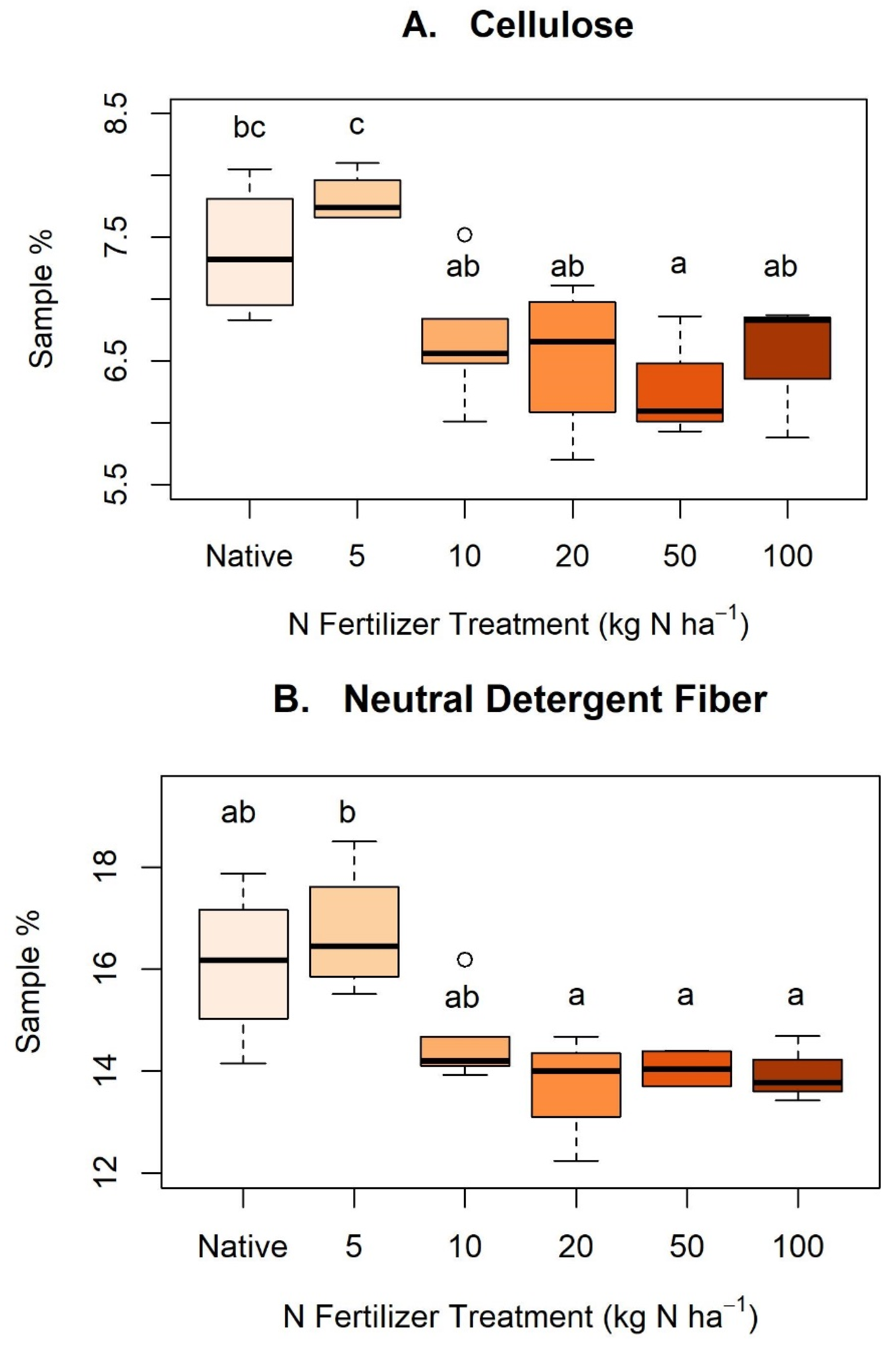
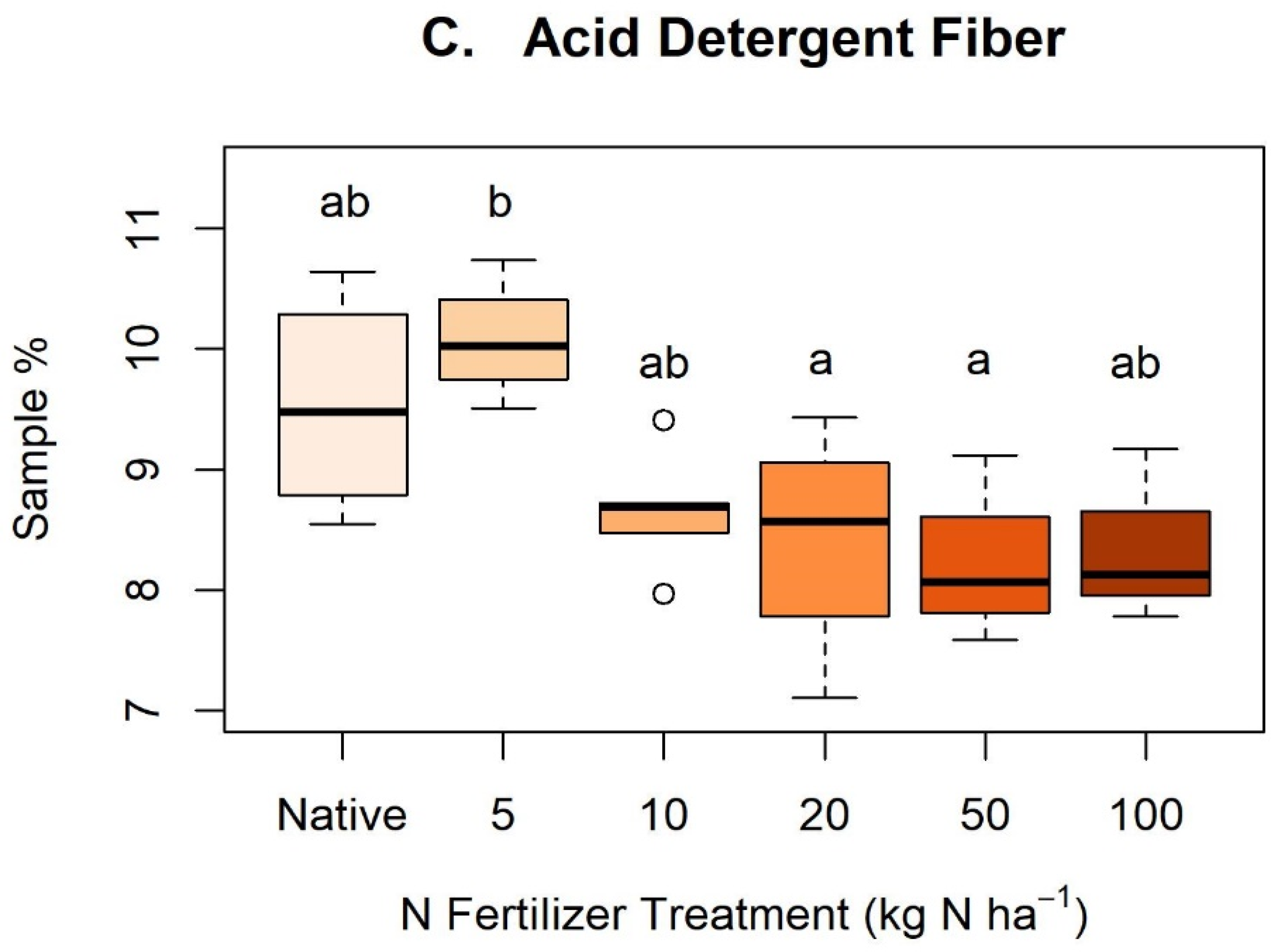
Dietary fibers showed a wide variety of concentrations between samples (Appendix B). We observed no difference in fiber concentrations between sampling period (t = −0.07 to 1.28, p > 0.05) except for HMC (t = −2.77, p = 0.01) where the first sampling period had significantly more HMC than the second sampling period. Similarly, we found no significant difference between sun and shaded leaf area in either May (t = −1.13, p = 0.27) or June (t = 0.29, p = 0.78), nor when sample dates were pooled (t = −0.88, p = 0.38). We found no statistically significant difference (p > 0.05) between N treatments and HMC, ADL, or AIA concentrations. CLL (F = 5.68, p < 0.01), NDF (F = 5.51, p < 0.01), and ADF (F = 4.19, p < 0.01) concentrations differed across N treatments (Appendix C).
3.1. Hyperspectral Vegetation Indices
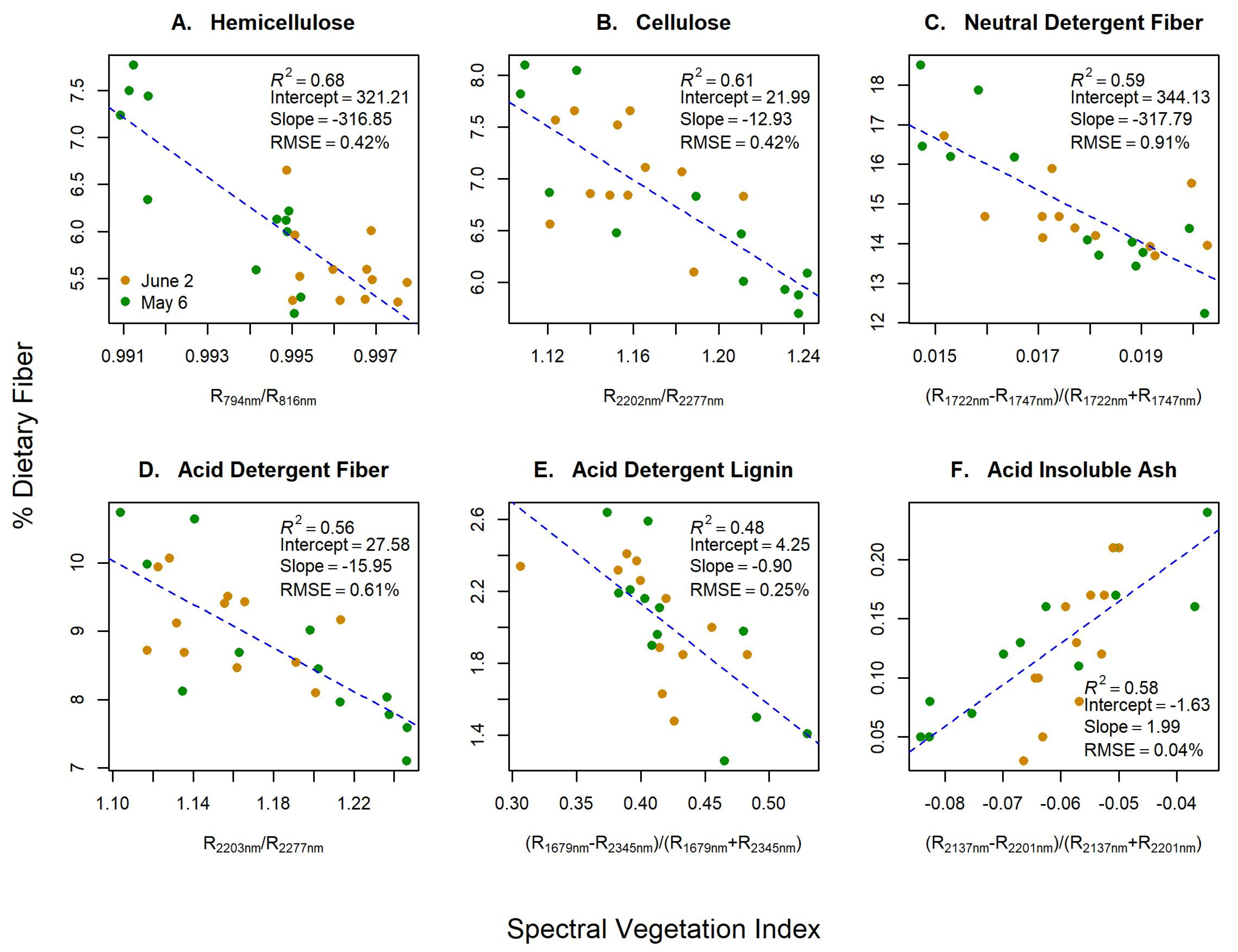
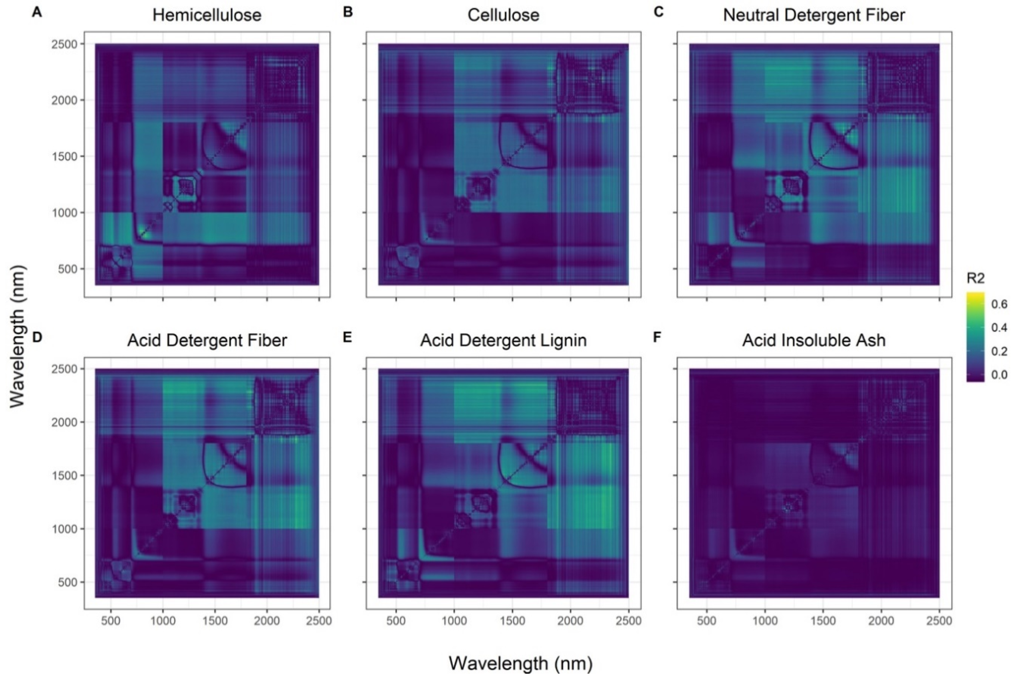
As hypothesized, the best SVIs for tracking dietary fibers contained bands >700 nm, with most wavelengths located in the SWIR region (R2 = 0.48–0.68; RMSE = 0.04–0.91%; Figure 2), but with viable SVIs occurring in the NIR region as well (Figure 3). HMC was the only fiber that was best predicted using a non-SWIR SVI (794 nm/816 nm). Cross validation scores were good ( = 0.73–0.83; Table 1), especially for a small sample size. However, all models underpredicted fiber concentration (slopes < 1). Additionally, we saw an improved model fit and predictive ability when adding shaded leaf area metrics to predict NDF (ΔAICc = −7.65; ΔLOOCV = +8%). Predictive ability also increased slightly when leaf area metrics were added to CLL (ΔLOOCV = +2–3%) and ADF models (ΔLOOCV = +1%), but without improvements in model fit. HMC models also improved (ΔAICc = −3.17; ΔLOOCV = +5%) when sun leaf area was added. No improvements in model fit or predictive power occurred for ADL, or AIA.
3.2. Band Equivalent Reflectance of WV-3
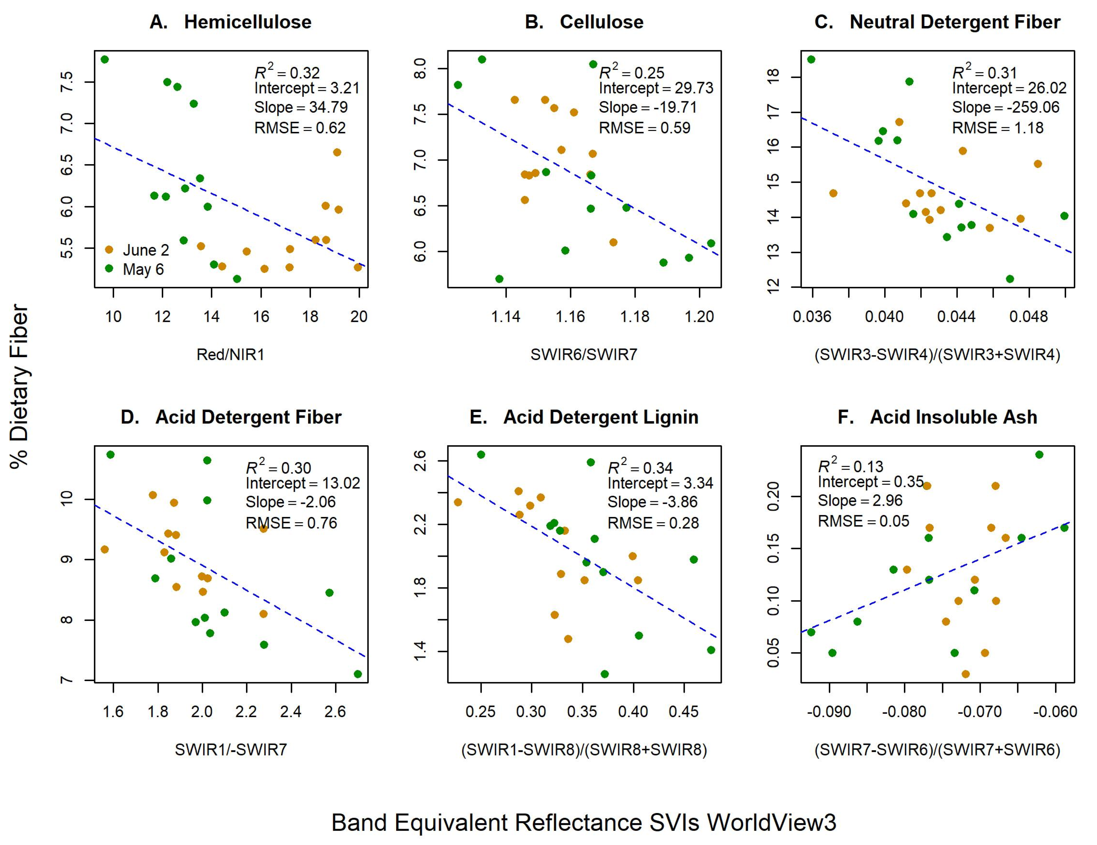
We convolved our hyperspectral data to the BER of WV-3 to assess whether dietary fibers could be measured via satellite (Table 2; Figure 4). As with the hyperspectral models, the majority of the best performing WV-3 SVIs contained SWIR bands (Figure 4). WV-3 models also underpredicted fiber concentration (slopes < 1) and performed poorer (R2 = 0.13–0.35; RMSE = 0.05–1.18%) than hyperspectral models (R2 = 0.48–0.68; RMSE = 0.04–0.91%). However, BER SVIs from WV-3 showed some promise in predicting HMC, NDF, and ADF, particularly when leaf area metrics were accounted for in the models (Table 2). As with the hyperspectral models, the best improvements in models came when shaded leaf area was added to NDF (R2 = 0.45; RMSE = 1.03%; LOOCV = 0.78) and ADF (R2 = 0.40; RMSE = 0.69%; LOOCV = 0.76). In contrast, HMC saw the best model improvements when total leaf area was added (R2 = 0.45; RMSE = 0.55%; LOOCV = 0.72). WV-3 models for CLL showed slight increase in cross validation scores when leaf area metrics were incorporated (ΔLOOCV = +4–5%), but without increased model fit or explained variance. ADL and AIA showed no model fit improvements with the addition of leaf area metrics, which was consistent with our hyperspectral results.
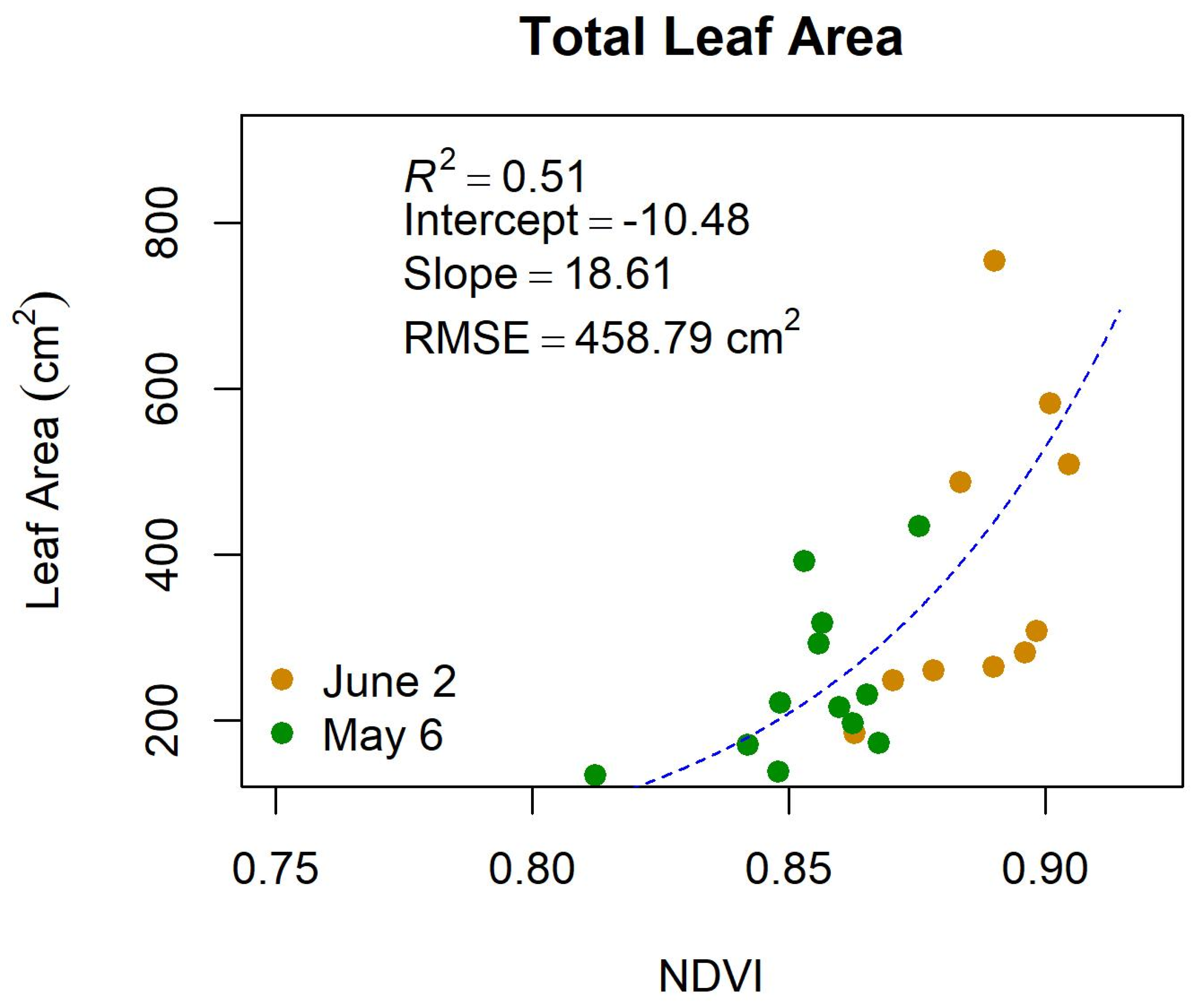
We also assessed how well total leaf area could be represented using NDVI in the WV-3 models. Results showed that total leaf area and NDVI had a nonlinear relationship with moderate strength (R2 = 0.51; RMSE = 458.79 cm2; Appendix D). When NDVI replaced total leaf area in WV-3 models, we found slight improvements predictive ability (ΔLOOCV = +1–2%; Appendix D) for HMC, CLL, ADF, ADL, and AIA, while NDF showed reduced predictive power (ΔLOOCV = −5%) compared to SVI only models.
4. Discussion
Our results indicate dietary fibers from an important forage species of arctic-boreal willow can be effectively measured with hyperspectral instruments. This finding supports previous work where dietary fibers have been successfully mapped in rangelands [28,29], grasslands [25,26], and mixed forest landscapes [27] using hyperspectral remote sensing. As hypothesized, all of the best performing SVIs contained wavelengths greater than 700 nm [22], with the majority of SVIs containing bands in the SWIR region [23,24].
Incorporating plant structure into hyperspectral models also improved our ability to track and predict HMC, NDF, and ADL (Table 1). This is likely related to the wavelengths used in the SVIs for these fibers. The NIR region is most sensitive to changes in plant structure with the initial portion of the SWIR region (1500–2000 nm) also showing sensitivity to changes in LAI [32]. In our study, all three of the fibers that showed improvements when leaf area was incorporated had at least one band in their SVIs in these regions. In contrast, the remaining three fibers—CLL, ADF, and AIA—all had SVIs in the latter part of the SWIR region (2000–2500 nm; Figure 2), which is less sensitive to plant structure [32]. Additionally, since the SWIR region is influenced by foliar water content, as water comprises 40–80% of weight in green specimens [23], future work may benefit from comparing spectral collections from wet and dry samples as this may improve model performance.
We observed model improvements from plant structure in HMC, NDF, and ADL depended on the partitioning leaf area into shaded and sunlit fractions. HMC models improved most when sunlit leaf area was added to models (Table 1). One study found that HMC was highly influenced by shade in two palatable shrubs—yaupon (Ilex vomitoria) and Japanese honeysuckle (Lonicera japonica)—where HMC levels were up to 92% more in sunlit plants than shaded comparisons [36]. However, due to constraints in the available dry matter for laboratory analyses in our study, we were unable to assess how fiber concentrations varied between sun and shaded leaves. In contrast, the best NDF and ADL models occurred when shaded leaf area was incorporated (Table 1). Again, this may be related to the relative amount of these fibers in sun vs. shaded leaves. ADL concentrations in yaupon and honeysuckle leaves were significantly higher in shaded plants [36]; however, one study found no statistical difference in lignin (ADL) between shaded and sunlit samples of diamond leaf willow [35]. This same study found that NDF was significantly higher in sunny willow shoots compared to shaded shoots [35], which would not explain why our NDF models improved most when shaded leaf area was included. However, other work has shown that NDF content in shaded and sunlit plants varies according to species, where some show higher NDF in shaded plants [55]. Thus, we anticipate that our results were specific to feltleaf willow and might not be generalized to other shrubs in high latitudes. Our results also suggest in addition to the importance of plant structural characteristics, the light environment plays a critical role in the development of these fibers in feltleaf willow. One remotely sensed product that may parse shaded and sunlit fractions of vegetation canopies is the Earth polychromatic imaging camera’s (EPIC) sunlit LAI product (10 km spatial resolution), although it is likely a finer spatial scale would be required to apply this product to high latitude settings as variations in LAI vary substantially across the landscape [56].
Sun-dependent variations in foliar biochemical composition influence herbivore foraging behavior. Snowshoe hares (Lepus americanus) preferred shaded browse shoots from feltleaf willow over sunlit comparisons [7]. Similarly, Sitka black-tailed deer (Odocoileus hemionus sitkensis) showed a preference for shade-grown Alaska blueberry (Vaccinium alaskensis) over those grown in sunlit clearcuts [57]. Indeed, it appears that digestibility and quality of forage in palatable high-latitude shrubs is greater in shaded plants [35,58]. This is likely linked to decreased light available for photosynthesis, which in turn may limit the formation of structural fibers [35,59] and increased foliar nitrogen and decreased defense compound concentrations [60].
Shrub proliferation in Arctic regions is increasing the range of herbivores such as snowshoe hare, moose (Alces alces), and ptarmigan (Lagopus lagopus, L. muta) [5,6]. Increases in ambient temperature may lower the digestibility of forage species by increasing lignification [61] and decreasing nitrogen in the late summer [12], but these changes are likely species and region specific [58,62]. Shading from clouds or canopy may improve forage quality [35,58,61]. However, studies have shown that warming may significantly alter forage quality for high latitude herbivores, which may have broader consequences for ecosystem functions such as nutrient cycling [12,13]. Thus, as warming continues, the palatability of shrubs in high latitudes will likely be a function of landscape structure, browsing intensity, and environmental conditions.
Strategies for monitoring variation in forage quality over broad heterogeneous landscapes are needed to account for changes over space and time. To this end, we evaluated the suitability the WV-3 satellite to measure dietary fibers and we predicted its eight SWIR bands would be useful in estimating dietary fibers. Of the eight SWIR bands, six of them comprised the best performing BER SVIs for CLL, NDF, ADF, ADL, and AIA (Figure 4). As with the hyperspectral models, the WV-3 models for HMC and NDF saw improvements when plant structural information was included, particularly when shaded leaf area was included (Table 2). However, we observed the best HMC model with total leaf area. We also observed that ADL predictions no longer benefitted from including leaf area but ADF models improved when shaded or total leaf area was included.
Few works have evaluated the utility of WorldView satellites for detecting foliar biochemical properties in high latitude regions. Our results suggest that WV-3 can estimate HMC, NDF, and ADF in a palatable high-latitude shrub with moderate accuracy when additional plant structural information is included in models, but that hyperspectral remote sensing approaches are best suited for mapping dietary fibers in feltleaf willow. Therefore, future work may benefit from assessing and using the upcoming German environmental mapping and analysis program (EnMAP) satellite. EnMAP will collect moderate spatial resolution (30 m) hyperspectral imagery (420–2450 nm) and make data freely available [63].
We also evaluated the possibility of using NDVI as a proxy for total leaf area in the WV-3 models (Appendix D). Although we found a moderate-strength nonlinear relationship between total leaf area and NDVI, only HMC showed improved model statistics when NDVI was included. This suggests that additional, non-spectral measures of shrub structure, and possibly leaf water content, may be necessary to pair with SVIs to obtain the best estimates of dietary fibers. Aerial lidar (light detection and ranging) may be used to represent LAI [64,65] and may increase our ability to map dietary fibers in high latitude regions when coupled with hyperspectral data.
Due to the controlled setting of our study, we did not evaluate the influence of soil background effects or confounding factors (e.g., shadows) on our ability to estimate dietary fibers. Similarly, the composite nature of all remotely sensed pixels includes spectral information from multiple constituents, which impedes our ability to remotely sense vegetation properties [66]. Therefore, techniques such as spectral mixture analysis [67] or combined spectral indices [68] may be needed to parse the spectral information of the variable of interest from background noise. For example, previous work has demonstrated the influence of soil properties on sensing foliar biochemical properties and plant structural characteristics such as LAI [69]. Finally, our study was limited by disease and pests in the greenhouse. Despite these afflictions that resulted in a small sample size, our results demonstrate the utility of hyperspectral and multispectral sensors to track dietary fibers in a high latitude palatable forage shrub.
5. Conclusions
This study contributed to an emerging need to estimate and monitor forage quality across wide expanses in high latitude systems. Results demonstrated that hyperspectral data is best suited to estimating dietary fibers in a palatable northern shrub and highlighted the importance of the SWIR region for this purpose. Additionally, information regarding plant structure and the light environment may augment our ability to estimate dietary fibers in these landscapes. Future work should evaluate the efficacy of including plant structure and light environment in addition to passive spectral information to estimate forage quality metrics in a field-based setting.
Author Contributions
Conceptualization, J.S.J., J.U.H.E., J.R.P. and L.A.V.; methodology, J.S.J., J.U.H.E., J.R.P. and L.A.V.; formal analysis, J.S.J.; resources, J.R.P.; writing—original draft preparation, J.S.J.; writing—review and editing, J.S.J., J.U.H.E., J.R.P. and L.A.V.; visualization, J.S.J.; funding acquisition, J.S.J., J.U.H.E., J.R.P. and L.A.V. All authors have read and agreed to the published version of the manuscript.
Funding
This research was funded by National Aeronautics and Space Administration’s (NASA) Arctic Boreal Vulnerability Experiment (ABoVE) grant numbers: NNX15AT89A and NNX15AW71A as well as NASA’s Idaho Space Grant Consortium (ISGC).
Acknowledgments
We sincerely thank Wayne Adkins, Ben Busack, Matt Lesiecki, Sarah Lewis, Don Regan, Amanda Stasiewicz, and Melissa Topping for their technical contributions and greenhouse assistance. We thank Pete Robichaud for the use of the FieldSpec Pro Full Range Spectroradiometer. Additionally, we thank Mark Hebblewhite for his expertise and guidance regarding forage quality.
Conflicts of Interest
The authors declare no conflict of interest.
Appendix A. Details on Nitrogen (N) Fertilizer Treatment Estimation
We estimated the native treatment N amount from soil samples collected adjacent to shrubs in the field (n = 3; 0–10 cm depth) and analyzed for total N and bulk density (g cm−3) in the lab. Since not all soil N is available for plant uptake, we assumed 39% of these values were estimated to be plant available N (i.e., ammonium (NH4+) or nitrate (NO3−)). This uptake percentage is in accordance with a previous study that estimated available N uptake from a deciduous shrub (Vaccinium uliginosum) in interior Alaska to be 39% of the soil N pool throughout the growing season (i.e., Chapin, 1983). Plant available, soil-organic N concentrations were calculated using the following equation:
where SON is soil organic N, BD is bulk density (g cm−3), and SD is soil depth (cm). The resultant values of soil organic N for available datasets were 36.40, 48.47, and 52.06 (kg ha−1). These estimated values were averaged and served as our estimate for native soil conditions (45.64 kg ha−1). All other fertilizer treatments were additions to this value.
SON (kg ha−1) = SON (%) × BD × SD × 1000
Appendix B. Summary Statistics for Dietary Fibers

Table A1.
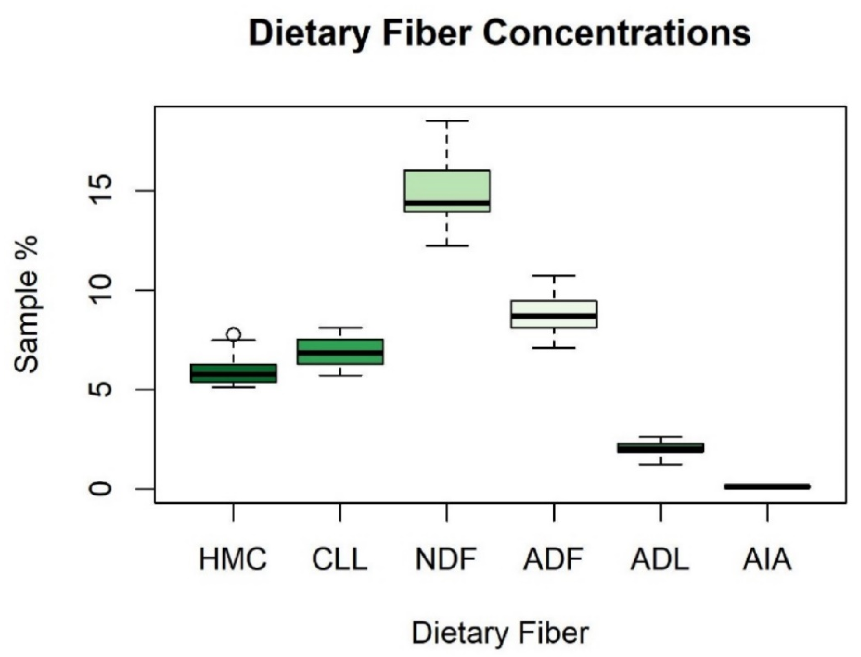
Table depicting summary statistics for dietary fibers: hemicellulose (HMC), cellulose (CLL), neutral detergent fiber (NDF), acid detergent fiber (ADF), acid detergent lignin (ADL), and acid insoluble ash (AIA).
Table A1.
Table depicting summary statistics for dietary fibers: hemicellulose (HMC), cellulose (CLL), neutral detergent fiber (NDF), acid detergent fiber (ADF), acid detergent lignin (ADL), and acid insoluble ash (AIA).
| Fiber | Range | Mean | Standard Deviation |
|---|---|---|---|
| HMC | 5.13–7.77% | 6.01% | 0.79% |
| CLL | 5.70–8.10% | 6.87% | 0.71% |
| NDF | 12.24–18.51% | 14.89% | 1.48% |
| ADF | 7.11–10.74% | 8.89% | 0.95% |
| ADL | 1.26–2.64% | 2.02% | 0.37% |
| AIA | 0.03–0.24% | 0.12% | 0.06% |
Figure A1.
Boxplot depicting summary statistics for dietary fibers: hemicellulose (HMC), cellulose (CLL), neutral detergent fiber (NDF), acid detergent fiber (ADF), acid detergent lignin (ADL), and acid insoluble ash (AIA).
Figure A1.
Boxplot depicting summary statistics for dietary fibers: hemicellulose (HMC), cellulose (CLL), neutral detergent fiber (NDF), acid detergent fiber (ADF), acid detergent lignin (ADL), and acid insoluble ash (AIA).

Appendix C. Nitrogen Treatments and Cellulose, Neutral Detergent Fiber, and Acid Detergent Fiber
Figure A2.
Boxplots depicting statistically significant differences (p < 0.05) between nitrogen (N) treatments and dietary fibers: (A) cellulose, (B) neutral detergent fiber, and (C) acid detergent fiber. Letters indicate statistically significant differences between groups within each figure but are not comparable across figures. No statistically significant differences were found between N treatments in hemicellulose, acid detergent lignin, or acid detergent ash.


Appendix D. Results of Swapping Leaf Area for the Normalized Difference Vegetation Index
Table A2.
Incorporating the normalized difference vegetation index (NDVI) as a proxy for leaf area into the best the band equivalent reflectance (BER) of WorldView3 (WV3) spectral vegetation index (SVI) results for hemicellulose, cellulose, neutral detergent fiber (NDF), acid detergent fiber (ADF), acid detergent lignin (ADL), and acid insoluble ash (AIA) and associated variance explained (R2), root mean square error (RMSE), Akaike’s information criterion for small sample sizes (ΔAICc), and leave-one-out cross validation (ΔLOOCV).
| Models | R2 | RMSE | AICc | ΔAICc | LOOCV Slope | LOOCV | ΔLOOCV |
|---|---|---|---|---|---|---|---|
| Hemicellulose (HMC) | |||||||
| SVI | 0.32 | 0.62% | 52.65 | - | 0.27 | 0.52 | - |
| SVI+ NDVI | 0.37 | 4.28% | 52.41 | −0.24 | 0.67 | 0.53 | +1% |
| Cellulose (CLL) | |||||||
| SVI | 0.25 | 0.59% | 50.10 | - | 0.22 | 0.45 | - |
| SVI+ NDVI | 0.21 | 0.59% | 53.00 | +2.90 | 0.14 | 0.47 | +5% |
| Neutral detergent fiber (NDF) | |||||||
| SVI | 0.31 | 1.18% | 83.33 | - | 0.26 | 0.67 | - |
| SVI+ NDVI | 0.28 | 1.18% | 86.09 | +2.76 | 0.22 | 0.62 | −5% |
| Acid detergent fiber (ADF) | |||||||
| SVI | 0.30 | 0.76% | 62.10 | - | 0.28 | 0.57 | - |
| SVI+ NDVI | 0.27 | 0.76% | 64.92 | +2.82 | 0.21 | 0.58 | +9% |
| Acid detergent lignin (ADL) | |||||||
| SVI | 0.34 | 0.28% | 15.05 | - | 0.33 | 0.70 | - |
| SVI+ NDVI | 0.34 | 0.28% | 16.99 | +1.94 | 0.33 | 0.71 | +1% |
| Acid detergent ash (AIA) | |||||||
| SVI | 0.13 | 0.05% | −66.35 | - | 0.11 | 0.31 | - |
| SVI+ NDVI | 0.13 | 0.05% | −64.44 | +1.91 | 0.07 | 0.33 | +2% |
Figure A3.
The relationship between total leaf area (cm2) and the normalized differenced vegetation index (NDVI) of the band equivalent reflectance of the WorldView3 satellite.
Figure A3.
The relationship between total leaf area (cm2) and the normalized differenced vegetation index (NDVI) of the band equivalent reflectance of the WorldView3 satellite.

References
- Serreze, M.C.; Walsh, J.E.; Chapin, F.S.I.; Osterkamp, T.; Dyurgerov, M.; Romanovsky, V.; Oechel, W.C.; Morison, J.; Zhang, T.; Barry, R.G. Observational evidence of recent change in the northern high- latitude environment. Clim. Chang. 2000, 46, 159–207. [Google Scholar] [CrossRef]
- Wolken, J.M.; Hollingsworth, T.N.; Rupp, T.S.; Chapin, F.S.; Trainor, S.F.; Barrett, T.M.; Sullivan, P.F.; McGuire, A.D.; Euskirchen, E.S.; Hennon, P.E.; et al. Evidence and implications of recent and projected climate change in Alaska’s forest ecosystems. Ecosphere 2011, 2, 1–35. [Google Scholar] [CrossRef]
- Myers-Smith, I.H.; Forbes, B.C.; Wilmking, M.; Hallinger, M.; Lantz, T.; Blok, D.; Tape, K.D.; Macias-fauria, M.; Sass-klaassen, U.; Esther, L. Shrub expansion in tundra ecosystems: Dynamics, impacts and research priorities. Environ. Res. Lett. 2011, 6, 045509. [Google Scholar] [CrossRef] [Green Version]
- Sturm, M.; Racine, C.; Tape, K.; Cronin, T.W.; Caldwell, R.L.; Marshall, J. Increasing shrub abundance in the Arctic. Nature 2001, 411, 546–547. [Google Scholar] [CrossRef]
- Tape, K.D.; Gustine, D.D.; Ruess, R.W.; Adams, L.G.; Clark, J.A. Range expansion of moose in Arctic Alaska linked to warming and increased shrub habitat. PLoS ONE 2016, 11, e0152636. [Google Scholar] [CrossRef] [PubMed]
- Zhou, J.; Tape, K.D.; Prugh, L.; Kofinas, G.; Carroll, G.; Kielland, K. Enhanced shrub growth in the Arctic increases habitat connectivity for browsing herbivores. Glob. Chang. Biol. 2020, 26, 3809–3820. [Google Scholar] [CrossRef]
- Bryant, J.P. Feltleaf willow-snowshoe hare interactions: Plant carbon/nutrient balance and floodplain succession. Ecology 1987, 68, 1319–1327. [Google Scholar] [CrossRef]
- Christie, K.S.; Bryant, J.P.; Gough, L.; Ravolainen, V.T.; Ruess, R.W.; Tape, K.D. The role of vertebrate herbivores in regulating shrub expansion in the Arctic: A synthesis. Bioscience 2015, 65, 1123–1133. [Google Scholar] [CrossRef] [Green Version]
- Butler, L.G.; Kielland, K. Acceleration of vegetation turnover and element cycling by mammalian herbivory in riparian ecosystems. J. Ecol. 2008, 96, 136–144. [Google Scholar] [CrossRef]
- Kielland, K.; Bryant, J.P. Moose herbivory in Taiga: Effects on biogeochemistry and vegetation dynamics in primary succession. OIKOS 1998, 82, 377–383. [Google Scholar] [CrossRef]
- Speed, J.D.M.; Austrheim, G.; Hester, A.J.; Mysterud, A.; Speed, J.D.M.; Austrheim, G.; Hester, A.J.; Mysterud, A. Experimental evidence for herbivore limitation of the treeline. Ecology 2010, 91, 3414–3420. [Google Scholar] [CrossRef] [PubMed]
- Doiron, M.; Gauthier, G.; Lévesque, E. Effects of experimental warming on nitrogen concentration and biomass of forage plants for an arctic herbivore. J. Ecol. 2014, 102, 508–517. [Google Scholar] [CrossRef]
- Zamin, T.J.; Côté, S.D.; Tremblay, J.P.; Grogan, P. Experimental warming alters migratory caribou forage quality. Ecol. Appl. 2017, 27, 2061–2073. [Google Scholar] [CrossRef] [PubMed]
- Felton, A.M.; Wam, H.K.; Stolter, C.; Mathisen, K.M.; Wallgren, M. The complexity of interacting nutritional drivers behind food selection, a review of northern cervids. Ecosphere 2018, 9, e02230. [Google Scholar] [CrossRef]
- Van Soest, P.J.; Robertson, J.B.; Lewis, B.A. Methods for dietary fiber, neutral detergent fiber, and non- starch polysaccharides in relation to animal nutrition. J. Dairy Sci. 1991, 74, 3583–3597. [Google Scholar] [CrossRef]
- Shipley, L.A.; Spalinger, D.E. Mechanics of browsing in dense food patches: Effects of plant and animal morphology on intake rate. Can. J. Zool. 1992, 70, 1743–1752. [Google Scholar] [CrossRef]
- Barboza, P.S.; Parker, K.L.; Hume, I.D. Integrative Wildlife Nutrition; Springer Science & Business Media: Berlin/Heidelberg, Germany, 2008. [Google Scholar]
- Xue, J.; Su, B. Significant remote sensing vegetation indices: A review of developments and applications. J. Sens. 2017. [Google Scholar] [CrossRef] [Green Version]
- Rouse, J.W., Jr.; Haas, R.H.; Schell, J.A.; Deering, D.W. Paper A 20. In Third Earth Resources Technology Satellite-1 Symposium: The Proceedings of A SYMPOSIUM Held by Goddard Space Flight Center at Washington, DC on 10–14 December 1973: Prepared at Goddard Space Flight Center; Scientific and Technical Information Office, National Aeronautics and Space Administration: Washington, DC, USA, 1974; Volume 351, p. 309. [Google Scholar]
- Doiron, M.; Legagneux, P.; Gauthier, G.; Lévesque, E. Broad-scale satellite Normalized Difference Vegetation Index data predict plant biomass and peak date of nitrogen concentration in Arctic tundra vegetation. Appl. Veg. Sci. 2013, 16, 343–351. [Google Scholar] [CrossRef]
- Johnson, H.E.; Gustine, D.D.; Golden, T.S.; Adams, L.G.; Parrett, L.S.; Lenart, E.A.; Barboza, P.S. NDVI exhibits mixed success in predicting spatiotemporal variation in caribou summer forage quality and quantity. Ecosphere 2018, 9, e02461. [Google Scholar] [CrossRef] [Green Version]
- Kokaly, R.F.; Asner, G.P.; Ollinger, S.V.; Martin, M.E.; Wessman, C.A. Characterizing canopy biochemistry from imaging spectroscopy and its application to ecosystem studies. Remote Sens. Environ. 2009, 113, 78–91. [Google Scholar] [CrossRef]
- Elvidge, C.D. Visible and near-infrared reflectance characteristics of dry plant materials. Int. J. Remote Sens. 1990, 11, 1775–1795. [Google Scholar] [CrossRef]
- Curran, P.J. Remote sensing of foliar chemistry. Remote Sens. Environ. 1989, 30, 271–278. [Google Scholar] [CrossRef]
- Wang, Z.; Townsend, P.A.; Schweiger, A.K.; Couture, J.J.; Singh, A.; Hobbie, S.E.; Cavender-bares, J. Mapping foliar functional traits and their uncertainties across three years in a grassland experiment. Remote Sens. Environ. 2019, 221, 405–416. [Google Scholar] [CrossRef]
- Knox, N.M.; Skidmore, A.K.; Prins, H.H.; Heitkönig, I.M.; Slotow, R.; van der Waal, C.; de Boer, W.F. Remote sensing of forage nutrients: Combining ecological and spectral absorption feature data. Isprs J. Photogramm. Remote Sens. 2012, 72, 27–35. [Google Scholar] [CrossRef]
- Asner, G.P.; Martin, R.E.; Carranza-jim, L.; Sinca, F.; Tupayachi, R.; Anderson, C.B.; Martinez, P. Functional and biological diversity of foliar spectra in tree canopies throughout the Andes to Amazon region. New Phytol. 2014, 204, 127–139. [Google Scholar] [CrossRef]
- Mirik, M.; Norland, J.E.; Crabtree, R.L.; Biondini, M.E. Hyperspectral one-meter-resolution remote sensing in Yellowstone National Park, Wyoming: I. Forage Nutritional Values. Soc. Range Manag. 2005, 58, 452–458. [Google Scholar] [CrossRef]
- Starks, P.J.; Coleman, S.W.; Phillips, W.A. Determination of forage chemical composition using remote sensing. J. Range Manag. 2004, 57, 635–640. [Google Scholar] [CrossRef]
- Chen, J.M.; Cihlar, J. Retrieving leaf area index of boreal conifer forests using landsat TM images. Remote Sens. Environ. 1996, 55, 153–162. [Google Scholar] [CrossRef]
- Turner, D.P.; Cohen, W.B.; Kennedy, R.E.; Fassnacht, K.S.; Briggs, J.M. Relationships between leaf area index and Landsat TM spectral vegetation indices across three temperate zone sites. Remote Sens. Environ. 1999, 70, 52–68. [Google Scholar] [CrossRef]
- Asner, G.P. Biophysical and biochemical sources of variability in canopy reflectance. Remote Sens. Environ. 1998, 64, 234–253. [Google Scholar] [CrossRef]
- Knyazikhin, Y.; Schull, M.A.; Stenberg, P.; Mõttus, M.; Rautiainen, M.; Yang, Y.; Marshak, A.; Carmona, P.L.; Kaufmann, R.K.; Lewis, P.; et al. Hyperspectral remote sensing of foliar nitrogen content. Proc. Natl. Acad. Sci. USA 2013, 110, E185–E192. [Google Scholar] [CrossRef] [PubMed] [Green Version]
- Vierling, L.A.; Deering, D.W.; Eck, T.F. Differences in arctic tundra vegetation type and phenology as seen using bidirectional radiometry in the early growing season. Remote Sens. Environ. 1997, 60, 71–82. [Google Scholar] [CrossRef]
- Molvar, E.M.; Bowyer, R.T.; Van Ballenberghe, V. Moose herbivory, browse quality, and nutrient cycling in an Alaskan treeline community. Oecologia 1993, 94, 472–479. [Google Scholar] [CrossRef] [PubMed]
- Blair, R.M.; Alcaniz, R.; Harrell, A. Shade intensity influences the nutrient quality and digestibility of southern deer browse leaves. J. Range Manag. 1983, 36, 257–264. [Google Scholar] [CrossRef]
- Zengeya, F.M.; Mutanga, O.; Murwira, A. Linking remotely sensed forage quality estimates from WorldView-2 multispectral data with cattle distribution in a savanna landscape. Int. J. Appl. Earth Obs. Geoinf. 2012, 21, 513–524. [Google Scholar] [CrossRef]
- Ramoelo, A.; Cho, M.A.; Mathieu, R.; Madonsela, S.; Van De Kerchove, R.; Kaszta, Z.; Wolff, E. Monitoring grass nutrients and biomass as indicators of rangeland quality and quantity using random forest modelling and WorldView-2 data. Int. J. Appl. Earth Obs. Geoinf. 2015, 43, 43–54. [Google Scholar] [CrossRef]
- Hively, W.D.; Lamb, B.T.; Daughtry, C.S.T.; Shermeyer, J.; Mccarty, G.W.; Quemada, M. Mapping crop residue and tillage intensity using WorldView-3 Satellite shortwave infrared residue indices. Remote Sens. 2018, 10, 1657. [Google Scholar] [CrossRef] [Green Version]
- Wu, H.; Levin, N.; Seabrook, L.; Moore, B.; Mcalpine, C. Mapping foliar nutrition using WorldView-3 and WorldView-2 to assess Koala habitat suitability. Remote Sens. 2019, 11, 215. [Google Scholar] [CrossRef] [Green Version]
- Liu, N.; Budkewitsch, P.; Treitz, P. Examining spectral reflectance features related to Arctic percent vegetation cover: Implications for hyperspectral remote sensing of Arctic tundra. Remote Sens. Environ. 2017, 192, 58–72. [Google Scholar] [CrossRef]
- Langford, Z.; Kumar, J.; Hoffman, F.M.; Norby, R.J.; Wullschleger, S.D.; Sloan, V.L.; Iversen, C.M. Mapping Arctic plant functional type distributions in the Barrow Environmental Observatory using WorldView-2 and LiDAR datasets. Remote Sens. 2016, 8, 733. [Google Scholar] [CrossRef] [Green Version]
- Dumroese, R.K.; Pinto, J.R.; Montville, M.E. Using container weights to determine irrigation needs: A simple method. Nativ. Plants J. 2015, 16, 67–71. [Google Scholar] [CrossRef]
- Schneider, C.A.; Rasband, W.S.; Eliceiri, K.W. NIH Image to ImageJ: 25 years of image analysis. Nat. Methods 2012, 9, 671–675. [Google Scholar] [CrossRef] [PubMed]
- Glozer, K. Protocol for Leaf Image Analysis—Surface Area. 2008. Available online: http//ucanr.edu/sites/fruittree/files/49325.pdf (accessed on 10 March 2020).
- R-Core Team. R: A Language and Environment for Statistical Computing; R Foundation for Statistical Computing: Vienna, Austria, 2013; Available online: http://www.r-project.org/ (accessed on 10 January 2019).
- Welch, B.L. The generalization of students’ problem when several different population variances are involved. Biometrika 1947, 34, 28–35. [Google Scholar] [PubMed]
- Tukey, J.W. Comparing individual means in the analysis of variance. Biometrics 1949, 5, 99–114. [Google Scholar] [CrossRef] [PubMed]
- Burnham, K.P.; Anderson, D.R. Model Selection and Multimodel Inference, 2nd ed.; Springer: New York, NY, USA, 2002. [Google Scholar]
- Cavanaugh, J.E. Unifying the derivations for the Akaike and corrected Akaike information criteria. Stat. Probab. Lett. 1997, 33, 201–208. [Google Scholar] [CrossRef]
- Barton, K.; Barton, M.K. Package ‘MuMIn’. 2015. Available online: https://cran.r-project.org/web/packages/MuMIn/MuMIn.pdf (accessed on 24 March 2020).
- Smith, A.M.S.; Wooster, M.J.; Drake, N.A.; Dipotso, F.M.; Falkowski, M.J.; Hudak, A.T. Testing the potential of multi-spectral remote sensing for retrospectively estimating fire severity in African Savannahs. Remote Sens. Environ. 2005, 97, 92–115. [Google Scholar] [CrossRef] [Green Version]
- Trigg, S.; Flasse, S. Characterizing the spectral-temporal response of burned savannah using in situ spectroradiometry and infrared thermometry. Int. J. Remote Sens. 2000, 21, 3161–3168. [Google Scholar] [CrossRef]
- Heiskanen, J. Estimating aboveground tree biomass and leaf area index in a mountain birch forest using ASTER satellite data. Int. J. Remote Sens. 2006, 27, 1135–1158. [Google Scholar] [CrossRef]
- Lin, C.H.; McGraw, M.L.; George, M.F.; Garrett, H.E. Nutritive quality and morphological development under partial shade of some forage species with agroforestry potential. Agrofor. Syst. 2001, 53, 269–281. [Google Scholar] [CrossRef]
- Juutinen, S.; Virtanen, T.; Kondratyev, V.; Laurila, T.; Linkosalmi, M.; Mikola, J.; Nyman, J.; Räsänen, A.; Tuovinen, J.P.; Aurela, M. Spatial variation and seasonal dynamics of leaf-Area index in the arctic tundra-implications for linking ground observations and satellite images. Environ. Res. Lett. 2017, 12, 095002. [Google Scholar] [CrossRef]
- Hanley, T.A. Physical and chemical response of understory vegetation to deer use in southeastern Alaska. Can. J. Res. 1987, 17, 195–199. [Google Scholar] [CrossRef]
- Lenart, E.A.; Bowyer, R.T.; Hoef, J.V.; Ruess, R.W. Climate change and caribou: Effects of summer weather on forage. Can. J. Zool. 2002, 80, 664–678. [Google Scholar] [CrossRef]
- Moore, K.J.; Jung, H.J.G. Lignin and fiber digestion. Rangel. Ecol. Manag. Range Manag. Arch. 2001, 54, 420–430. [Google Scholar] [CrossRef]
- Osier, T.L.; Lindroth, R.L. Effects of light and nutrient availability on Aspen: Growth, phytochemistry, and insect performance. J. Chem. Ecol. 1999, 25, 1687–1714. [Google Scholar]
- Weladji, R.B.; Klein, D.R.; Holand, Ø. Mysterud, a Comparative response of Rangifer tarandus and other northern ungulates to climatic variability. Rangifer 2002, 22, 33–50. [Google Scholar] [CrossRef] [Green Version]
- Elmendorf, S.C.; Henry, G.H.R.; Hollister, R.D.; Björk, R.G.; Bjorkman, A.D.; Callaghan, T.V.; Collier, L.S.; Cooper, E.J.; Cornelissen, J.H.C.; Day, T.A.; et al. Global assessment of experimental climate warming on tundra vegetation: Heterogeneity over space and time. Ecol. Lett. 2012, 15, 164–175. [Google Scholar] [CrossRef]
- Guanter, L.; Kaufmann, H.; Segl, K.; Foerster, S.; Rogass, C.; Chabrillat, S.; Kuester, T.; Hollstein, A.; Rossner, G.; Chlebek, C.; et al. The EnMAP spaceborne imaging spectroscopy mission for earth observation. Remote Sens. 2015, 7, 8830–8857. [Google Scholar] [CrossRef] [Green Version]
- Jensen, J.L.R.; Humes, K.S.; Vierling, L.A.; Hudak, A.T. Discrete return lidar-based prediction of leaf area index in two conifer forests. Remote Sens. Environ. 2008, 112, 3947–3957. [Google Scholar] [CrossRef] [Green Version]
- Pope, G.; Treitz, P. Leaf Area Index (LAI) estimation in boreal mixedwood forest of Ontario, Canada using Light detection and ranging (LiDAR) and worldview-2 imagery. Remote Sens. 2013, 5, 5040–5063. [Google Scholar] [CrossRef] [Green Version]
- Somers, B.; Asner, G.P.; Tits, L.; Coppin, P. Endmember variability in Spectral Mixture Analysis: A review. Remote Sens. Environ. 2011, 115, 1603–1616. [Google Scholar] [CrossRef]
- Adams, J.B.; Smith, M.O. Spectral mixture modeling: A new analysis of rock and soil types at the Viking Lander 1 site. J. Geophys. Res. 1986, 91, 8098–8112. [Google Scholar] [CrossRef]
- Eitel, J.U.H.; Long, D.S.; Gessler, P.E.; Hunt, E.R.; Brown, D.J. Sensitivity of ground-based remote sensing estimates of wheat chlorophyll content to variation in soil reflectance. Soil Sci. Soc. Am. 2009, 73, 1715–1723. [Google Scholar] [CrossRef] [Green Version]
- Darvishzadeh, R.; Skidmore, A.; Atzberger, C.; van Wieren, S. Estimation of vegetation LAI from hyperspectral reflectance data: Effects of soil type and plant architecture. Int. J. Appl. Earth Obs. Geoinf. 2008, 10, 358–373. [Google Scholar] [CrossRef]
Figure 1.
Experimental and data collection set up. Willows were grown in a greenhouse setting (A) and canopy spectra were collected using an FieldSpec Pro Full Range Spectroradiometer (C). A spectrally flat black-foam material below the canopy to avoid introducing soil and background noise (B).
Figure 1.
Experimental and data collection set up. Willows were grown in a greenhouse setting (A) and canopy spectra were collected using an FieldSpec Pro Full Range Spectroradiometer (C). A spectrally flat black-foam material below the canopy to avoid introducing soil and background noise (B).

Figure 2.
Spectral vegetation indices (SVIs) from hyperspectral data for green dietary fibers concentrations (Y-axis) of (A) hemicellulose, (B) cellulose, (C) neutral detergent fiber, (D) acid detergent fiber, (E) acid detergent lignin, and (F) acid insoluble ash. X-axis labels represent the measured reflectance (R) at given wavelengths in nanometers of SVIs.

Figure 3.
Coefficients of determination (R2) between green dietary fibers, (A) hemicellulose (HMC), (B) cellulose (CLL), (C) neutral detergent fiber (NDF), (D) acid detergent fiber (ADF), (E) acid detergent lignin (ADL), and (F) acid insoluble ash (AIA) and spectral vegetation indices (SVIs) generated from hyperspectral data. The x- and y-axes are the wavelength (nm) from the spectrometer. The best performing SVIs were for HMC, for CLL, ( for NDF, for ADF, ( for ADL, and ( for AIA—where R represents the measured reflectance at given wavelengths in nanometers.

Figure 4.
Band equivalent reflectance of WorldView-3 (WV-3) spectral vegetation indices (SVIs) for green dietary fibers concentrations (Y-axis) of (A) hemicellulose, (B) cellulose, (C) neutral detergent fiber, (D) acid detergent fiber, (E) acid detergent lignin, and (F) acid insoluble ash. X-axis labels represent the WV-3 bands used to create the best performing SVIs, and contain red, near infrared-1 (NIR1), and shortwave infrared (SWIR) bands.

Table 1.
Best performing hyperspectral vegetation index (SVI) results for hemicellulose, cellulose, neutral detergent fiber, acid detergent fiber, acid detergent lignin, and acid insoluble ash and associated variance explained (R2), root mean square error (RMSE), Akaike’s information criterion for small sample sizes (ΔAICc), and leave-one-out cross validation (LOOCV) slope and Spearman rank coefficients (). The first row of each section indicates model statistics for just the SVI model, while subsequent rows show how model statistics change when adding leaf area (LA) from the top of the canopy (sun), bottom of the canopy (shade), or combined sun and shade leaves (total). Comparisons of ΔAICc and ΔLOOCV are in reference to the SVI model only for each fiber.
| Models | R2 | RMSE | AICc | ΔAICc | LOOCV Slope | LOOCV | ΔLOOCV |
|---|---|---|---|---|---|---|---|
| Hemicellulose (HMC) | |||||||
| SVI | 0.68 | 0.42 | 34.62 | - | 0.66 | 0.73 | - |
| SVI+ LA Sun | 0.74 | 0.37 | 31.45 | −3.17 | 0.75 | 0.69 | −4% |
| SVI+ LA Shade | 0.69 | 0.41 | 35.48 | +0.86 | 0.68 | 0.77 | +4% |
| SVI+ LA Total | 0.72 | 0.39 | 32.63 | −1.99 | 0.71 | 0.73 | 0 |
| Cellulose (CLL) | |||||||
| SVI | 0.61 | 0.42 | 34.48 | - | 0.59 | 0.78 | - |
| SVI+ LA Sun | 0.59 | 0.43 | 37.14 | +2.69 | 0.56 | 0.80 | +2% |
| SVI+ LA Shade | 0.60 | 0.42 | 36.90 | +2.42 | 0.55 | 0.81 | +3% |
| SVI+ LA Total | 0.60 | 0.42 | 36.97 | +2.49 | 0.56 | 0.81 | +3% |
| Neutral detergent fiber (NDF) | |||||||
| SVI | 0.51 | 0.99 | 75.30 | - | 0.57 | 0.79 | - |
| SVI+ LA Sun | 0.55 | 0.93 | 74.82 | −0.40 | 0.59 | 0.81 | +2% |
| SVI+ LA Shade | 0.67 | 0.80 | 67.65 | −7.65 | 0.62 | 0.87 | +8% |
| SVI+ LA Total | 0.62 | 0.86 | 71.02 | −4.28 | 0.60 | 0.85 | +6% |
| Acid detergent fiber (ADF) | |||||||
| SVI | 0.56 | 0.61 | 51.31 | - | 0.53 | 0.75 | - |
| SVI+ LA Sun | 0.53 | 0.61 | 54.15 | +2.84 | 0.48 | 0.76 | +1% |
| SVI+ LA Shade | 0.53 | 0.61 | 54.20 | +2.89 | 0.50 | 0.75 | 0 |
| SVI+ LA Total | 0.53 | 0.61 | 54.17 | +2.86 | 0.49 | 0.76 | +1% |
| Acid detergent lignin (ADL) | |||||||
| SVI | 0.48 | 0.25 | 9.46 | - | 0.49 | 0.83 | - |
| SVI+ LA Sun | 0.49 | 0.25 | 10.86 | +1.46 | 0.51 | 0.82 | −1% |
| SVI+ LA Shade | 0.51 | 0.24 | 9.87 | +0.41 | 0.52 | 0.82 | −1% |
| SVI+ LA Total | 0.51 | 0.24 | 10.07 | +0.61 | 0.52 | 0.82 | −1% |
| Acid detergent ash (AIA) | |||||||
| SVI | 0.58 | 0.04 | −83.54 | - | 0.57 | 0.81 | - |
| SVI+ LA Sun | 0.56 | 0.04 | −82.77 | +0.84 | 0.55 | 0.81 | 0 |
| SVI+ LA Shade | 0.58 | 0.04 | −81.94 | +1.60 | 0.58 | 0.81 | 0 |
| SVI+ LA Total | 0.56 | 0.04 | −80.73 | +2.81 | 0.55 | 0.81 | 0 |
Table 2.
Best performing band equivalent reflectance (BER) of WorldView3 (WV3) spectral vegetation index (SVI) results for hemicellulose, cellulose, neutral detergent fiber, acid detergent fiber, acid detergent lignin, and acid insoluble ash and associated variance explained (R2), root mean square error (RMSE), Akaike’s information criterion for small sample sizes (ΔAICc), and leave-one-out cross validation (LOOCV) slope and Spearman rank correlations (). The first row of each section indicates model statistics for just the SVI model, while subsequent rows show how model statistics change when adding leaf area (LA) from the top of the canopy (sun), bottom of the canopy (shade), or combined sun and shade leaves (total). Comparisons of ΔAICc and ΔLOOCV are in reference to the SVI model only for each fiber.
| Models | R2 | RMSE | AICc | ΔAICc | LOOCV Slope | LOOCV | ΔLOOCV |
|---|---|---|---|---|---|---|---|
| Hemicellulose (HMC) | |||||||
| SVI | 0.32 | 0.62 | 52.65 | - | 0.27 | 0.52 | - |
| SVI+ LA Sun | 0.41 | 0.56 | 50.74 | −1.91 | 0.39 | 0.72 | +20% |
| SVI+ LA Shade | 0.40 | 0.57 | 51.38 | −1.27 | 0.38 | 0.72 | +20% |
| SVI+ LA Total | 0.45 | 0.55 | 49.29 | −3.36 | 0.43 | 0.72 | +20% |
| Cellulose (CLL) | |||||||
| SVI | 0.25 | 0.59 | 50.10 | - | 0.22 | 0.45 | - |
| SVI+ LA Sun | 0.23 | 0.59 | 52.44 | +2.34 | 0.20 | 0.50 | +5% |
| SVI+ LA Shade | 0.22 | 0.59 | 52.66 | +2.56 | 0.18 | 0.49 | +4% |
| SVI+ LA Total | 0.23 | 0.58 | 52.44 | +2.34 | 0.19 | 0.49 | +4% |
| Neutral detergent fiber (NDF) | |||||||
| SVI | 0.31 | 1.18 | 83.33 | - | 0.26 | 0.67 | - |
| SVI+ LA Sun | 0.33 | 1.14 | 84.34 | +1.01 | 0.31 | 0.71 | +4% |
| SVI+ LA Shade | 0.45 | 1.03 | 79.82 | −3.51 | 0.43 | 0.78 | +11% |
| SVI+ LA Total | 0.39 | 1.08 | 82.09 | −1.24 | 0.37 | 0.78 | +11% |
| Acid detergent fiber (ADF) | |||||||
| SVI | 0.30 | 0.76 | 62.10 | - | 0.28 | 0.57 | - |
| SVI+ LA Sun | 0.34 | 0.72 | 62.40 | +0.30 | 0.35 | 0.66 | +9% |
| SVI+ LA Shade | 0.40 | 0.69 | 60.43 | −2.33 | 0.38 | 0.76 | +19% |
| SVI+ LA Total | 0.38 | 0.70 | 60.92 | −2.82 | 0.38 | 0.73 | +16% |
| Acid detergent lignin (ADL) | |||||||
| SVI | 0.34 | 0.28 | 15.05 | - | 0.33 | 0.70 | - |
| SVI+ LA Sun | 0.32 | 0.28 | 17.51 | +2.46 | 0.32 | 0.71 | +1% |
| SVI+ LA Shade | 0.34 | 0.28 | 17.00 | +1.95 | 0.33 | 0.71 | +1% |
| SVI+ LA Total | 0.33 | 0.28 | 17.19 | +2.14 | 0.33 | 0.69 | −1% |
| Acid detergent ash (AIA) | |||||||
| SVI | 0.13 | 0.05 | −66.35 | - | 0.11 | 0.31 | - |
| SVI+ LA Sun | 0.09 | 0.05 | −63.45 | +2.90 | 0.08 | 0.31 | 0 |
| SVI+ LA Shade | 0.10 | 0.05 | −63.78 | +2.57 | 0.09 | 0.31 | 0 |
| SVI+ LA Total | 0.09 | 0.05 | −63.54 | +2.81 | 0.08 | 0.28 | −3% |
© 2020 by the authors. Licensee MDPI, Basel, Switzerland. This article is an open access article distributed under the terms and conditions of the Creative Commons Attribution (CC BY) license (http://creativecommons.org/licenses/by/4.0/).
Share and Cite
MDPI and ACS Style
Jennewein, J.S.; Eitel, J.U.H.; Pinto, J.R.; Vierling, L.A. Toward Mapping Dietary Fibers in Northern Ecosystems Using Hyperspectral and Multispectral Data. Remote Sens. 2020, 12, 2579. https://0-doi-org.brum.beds.ac.uk/10.3390/rs12162579
AMA Style
Jennewein JS, Eitel JUH, Pinto JR, Vierling LA. Toward Mapping Dietary Fibers in Northern Ecosystems Using Hyperspectral and Multispectral Data. Remote Sensing. 2020; 12(16):2579. https://0-doi-org.brum.beds.ac.uk/10.3390/rs12162579
Chicago/Turabian StyleJennewein, Jyoti S., Jan U.H. Eitel, Jeremiah R. Pinto, and Lee A. Vierling. 2020. "Toward Mapping Dietary Fibers in Northern Ecosystems Using Hyperspectral and Multispectral Data" Remote Sensing 12, no. 16: 2579. https://0-doi-org.brum.beds.ac.uk/10.3390/rs12162579
Note that from the first issue of 2016, this journal uses article numbers instead of page numbers. See further details here.