A Novel Method for the Deblurring of Photogrammetric Images Using Conditional Generative Adversarial Networks


Department of Geodesy, Faculty of Civil and Environmental Engineering, Gdansk University of Technology, Narutowicza 11-12, 80-233 Gdansk, Poland
Remote Sens. 2020, 12(16), 2586; https://0-doi-org.brum.beds.ac.uk/10.3390/rs12162586
Submission received: 13 July 2020
/
Revised: 9 August 2020
/
Accepted: 10 August 2020
/
Published: 11 August 2020
(This article belongs to the Special Issue Unmanned Aerial Vehicles for Photogrammetry)
Abstract
:The visual data acquisition from small unmanned aerial vehicles (UAVs) may encounter a situation in which blur appears on the images. Image blurring caused by camera motion during exposure significantly impacts the images interpretation quality and consequently the quality of photogrammetric products. On blurred images, it is difficult to visually locate ground control points, and the number of identified feature points decreases rapidly together with an increasing blur kernel. The nature of blur can be non-uniform, which makes it hard to forecast for traditional deblurring methods. Due to the above, the author of this publication concluded that the neural methods developed in recent years were able to eliminate blur on UAV images with an unpredictable or highly variable blur nature. In this research, a new, rapid method based on generative adversarial networks (GANs) was applied for deblurring. A data set for neural network training was developed based on real aerial images collected over the last few years. More than 20 full sets of photogrammetric products were developed, including point clouds, orthoimages and digital surface models. The sets were generated from both blurred and deblurred images using the presented method. The results presented in the publication show that the method for improving blurred photo quality significantly contributed to an improvement in the general quality of typical photogrammetric products. The geometric accuracy of the products generated from deblurred photos was maintained despite the rising blur kernel. The quality of textures and input photos was increased. This research proves that the developed method based on neural networks can be used for deblur, even in highly blurred images, and it significantly increases the final geometric quality of the photogrammetric products. In practical cases, it will be possible to implement an additional feature in the photogrammetric software, which will eliminate unwanted blur and allow one to use almost all blurred images in the modelling process.
1. Introduction
Unmanned aerial vehicle (UAV) photogrammetry and remote sensing have become very popular in recent years. UAVs as platforms for support research equipment enable reaching various regions and terrains, often inaccessible to traditional manned solutions. Their trajectory can be remotely controlled by humans or programmed and implemented automatically. The development and operation of commercial unmanned aerial vehicles is rapid and has become very simple owing to their commercialization. Within a short period, scientists and engineers from all over the world noticed these advantages and widely began using these devices to transport research equipment. As a result, engineering measurements and tests started to be conducted in new places with unprecedented frequency.
Commercial UAVs are the machines most commonly used for low-altitude photogrammetry. Their maximum take-off mass (MTOM) is low, typically not exceeding 25 kg, as is their capacity for carrying additional load. This enforces the need to reduce the weight of all components carried by such a vehicle. Miniaturization involves, among others, global navigation satellite system (GNSS) receivers, inertial navigation systems (INSs) and optoelectronic sensors (visible light, thermal imaging, and multispectral cameras), often making these devices less sophisticated and accurate. Unmanned platforms most commonly use single-frequency GNSS receivers, with a positioning accuracy of up to several meters [1,2,3]. Only recently have the engineers started fitting UAVs also with GNSS RTK (Real Time Kinematic) and PPK (Post-Processed kinematic) precise satellite navigation receivers, where the achieved accuracies are already at a level of 0.10 m [4,5,6,7]. Inertial sensors based on micro electromechanical systems (MEMSs) are used in relation to determining the UAV angular orientation values. The accuracy of determining angular values in inertial units of this type varies around 1° for transverse and longitudinal inclination angles, and 2° for the torsional angle [8]. Optoelectronic cameras carried by UAVs are small structures based on CMOS (Complementary Metal-Oxide-Semiconductor) sensors, CCDs (charge-coupled devices) or uncooled VOx (Vanadium Oxide) microbolometers, equipped with prime lens with a conical field of view. These are mainly non-metric cameras, where the internal orientation elements are not stable [9].
The photogrammetric process involves numerous factors impacting the quality of the end result [10,11,12,13,14,15,16,17,18,19]. In the course of research described herein, they were divided into three groups:
- Procedural—All elements of the image and additional data collection process, which originate from the adopted execution method and its correctness. This group contains the parameters of the applied flight plan (altitude, coverage, selected flight path and camera position), GNSS measurement accuracy (RTK), selected time of day, scenery illumination quality, etc.;
- Technical—Factors impacting the study quality, arising from the technical parameters of the devices used to collect data. This group contains the parameters and technical capabilities of the cameras, lens, stabilization systems, satellite navigation system receivers, etc.;
- Numerical—Factors originating from the methods and algorithms applied for digital data processing.
Maintaining the compilation quality requires good knowledge in the field of the aforementioned elements and their skillful balancing, as well as matching them with encountered measurement condition and faced requirements. If one of these groups remains unchanged (e.g., the technical one), the assumed quality requirements can be maintained by adjusting the parameters of other groups. In other words, with available constant technical resources, it is possible to adjust the numerical methods and procedures so as to achieve the objective. For example, if one has a given UAV with a specific camera and lens (fixed element), it is possible to match the flight altitude to achieve the required ground sampling distance (GSD). Otherwise, when it is impossible to change the flight altitude, which means that the procedural factor is constant, one can use another camera (lens and spatial resolution) or, alternatively, apply numerical methods in order to achieve the required GSD.
With the available constant technical element, the parameters of the procedural and numerical groups are adapted in order to reach the accuracy-related requirements of the outcome. The quality of the study can be significantly improved by properly selecting these elements. Some of them are determined analytically, at the task execution planning stage, e.g., flight altitude, speed, shutter speed, etc., while others are the result of agreed principles and adopted good practices. They primarily result from conducted research and gained experience. The research [20] presents the impact of significant coverage on the quality of point clouds generated within the photogrammetric process. The paper [21] discusses the results of experiments involving various flight plans and assesses their impact on the geometric quality of the developed models. The case study [22] reviews the results of a study originating from air and ground image data. The research [23] combines point clouds from terrestrial laser scanning (TLS) and ground image data. Similarly, the experiment [24] utilized the technique of fusing data from aerial laser scanning and optical sensors mounted on a single unmanned aerial platform. The authors of the publication [25] maximize aircraft performance, and in [26] put emphasis on flight correctness and proper planning. Several interesting scenarios and recommendations in terms of spatial modelling techniques were thoroughly discussed in [27].
It should be noted that an appropriate procedure for acquiring photos and its parameters (flight plan and its parameters) must be selected prior to their physical execution. However, there may be cases where the photos had already been taken, do not meet the assumed requirements and it is impossible to repeat the measurement. In general, it can be assumed that two elements impacting the quality of a photogrammetric study are constant, namely procedural, which is the inability to repeat a procedure with other parameters, and technical, which is the inability to change the technical parameters of the used measuring equipment. In such cases, in order to achieve a required study quality, one can apply specific numerical methods. Therefore, the result quality can be improved by using numerical methods. The author of [28] managed to significantly reduce ground sample distance and increased numbers of points in the dense point cloud using a fixed camera and flight altitude. The papers [13,16,18] review a method for improving the radiometric quality of photos. In [29], the researchers presented a method to improve the camera’s internal orientation elements and their impact on reconstruction quality. In the work [30], the results of improving a digital terrain model using the Monte Carlo method were reviewed. The authors of [31] discuss a thorough impact analysis regarding various feature detectors as well as reconstruction accuracy, whereas the publication [32] presents a new algorithm for the integration of dense image matching results from multiple stereo pairs.
The data acquisition process may encounter a situation in which blur appears on the images. Deblurring in aviation cameras is achieved by a forward motion compensation system (FMC), and blurring is due to aircraft or satellite forward motion [33]. For this purpose, analogue cameras have a mobile image plane, which mechanically compensates for the camera’s forward motion [34]. This compensation is known as time delayed integration (TDI) [35,36,37,38,39]. Blur compensation systems require precise synchronization with the vehicle’s navigation systems. Such solutions are not used in small and inexpensive cameras on commercial UAVs.
Image blurring caused by camera motion during exposure significantly impacts the photogrammetric process quality [40]. On blurred images it is difficult to visually locate ground control points, and the number of identified feature points decreases rapidly together with increasing blur kernel [26,41]. Hence, improving a blurred image can increase the number of detected features and, consequently, the geometric quality of generated point clouds and spatial models.
The authors of [42] divided deblurring methods into two groups, namely blind [43,44] and non-blind deconvolutions [45,46]. Both solutions are aimed at eliminating blur; however, the non-blind convolutions utilize information on the nature of the blur within an image, hence matching its elimination method. Blind methods do not have such knowledge. A different division is suggested by the authors of [47], who put them into seven groups, which are edge sharpness analysis, depth of field, blind de-convolution, Bayes discriminant function, non-reference block, lowest directional frequency energy and wavelet-based histogram. Apart from the aforementioned groups, there are also sensor-assisted blur detection [40,42,48,49] and the latest neural methods [50,51,52,53,54,55,56,57,58,59,60,61,62,63,64,65].
The methods for eliminating blur formed on aviation images assume that blur is of a linear nature, which is the case most often. This assumption is also adopted by FMC systems. When obtaining data using a UAV, the flight can be performed according to highly varied plans, at varying altitudes and distances to the object, and in different lighting conditions [66]. For this reason, the nature of blur can be non-uniform, which makes it hard to forecast [67,68]. Due to the above, the author of this publication concluded that the neural methods developed in recent years were able to eliminate blur on UAV images with an unpredictable or highly variable blur nature.
This paper presents the following new solutions in the field of photogrammetry and remote sensing:
- A new, rapid method based on generative adversarial networks (GANs) was applied for deblurring;
- A GAN network model was selected and applied, which can be implemented in UAVs and activated in real-time (highly practical significance of the solution);
- A set of neural network training data was developed based on real aerial images, collected by the author of the study over the last few years;
- More than 20 full sets of photogrammetric products were generated, including point clouds, orthoimages and the digital surface models, from blurred photos and photos subjected to the presented method;
- Techniques for improving photogrammetric photo quality were grouped and a tri-element model of a photogrammetric survey quality was presented.
The publication is divided into four sections. The Section 1 is the Introduction, which presents motivation behind the research. The Section 2, Materials and Methods, describes tools and methods used to process the data. Section 3 presents and discusses the obtained results. The paper ends with the Conclusions, where the most important aspects of the research are discussed and summarized.
2. Materials and Methods
2.1. Deblurring Method
A heterogeneous image blur model can be expressed as the following equation:
where represents an image with blur, are unknown blur kernels determined by a motion field M, represents a sharp latent image, and N is the additive noise. The * symbol means convolution.
Early deblurring methods required the knowledge of the k(M) function, which means they can be classified as non-blind deconvolution methods. In order to perform deconvolution and obtain an image , they were primarily based on Lucy–Richardson algorithms [69] and Wiener [70] or Tikhonov [71]. In the case of images obtained by commercial UAVs, we assume that the blur function is unknown. As already mentioned, inexpensive non-metric cameras are not fitted with any technical devices for blur kernel estimation. In such a case, it can be assumed that the application blind deblurring methods, which estimate the blur kernel k(M) can lead to obtaining a latent image . Unfortunately, these methods are intended for images with uniform blur, generated as a result of uniform camera motion relative to the object or background [72,73,74,75]. In the case of UAV images, assuming that the k(M) function is the same for the entire image surface is a great simplification and can lead to erroneous results. Some authors have identified this issue and are working on numerical methods based on a non-uniform blur model. The publications [76,77] present a non-uniform blind deblurring model based on a parametric geometric model of the blur process, which additionally takes camera rotation into account. The paper [78] assumes that blur is induced by a complex spatial motion of the camera. Therefore, it can be assumed that the estimation of the k(M) function for UAV images, taking into account all possible flight plans and cases is a very difficult task.
A rapid development of neural methods has been observed in recent years. Many of these have been successfully applied in photogrammetry and remote sensing [79]. Convolutional neural networks (CNNs) have been successfully used for eliminating blur [59,80,81,82,83]. In such solutions, the networks are trained using image pairs. Such pairs form sharp images with synthetically applied blur. Hence, CNNs are trained to estimate the blur kernel, which is then used for deconvolution.
The aforementioned methods estimate the blur kernel or assume its certain nature, followed by deconvolution. Another approach includes generating synthetic images without blur, based on their blurred counterparts. The task of converting one image type to another has only been made possible recently and can be implemented owing to generative adversarial networks (GANs) [84]. For example, a network generates an image based on a certain tag fed at the input [85]. Thus, in the case of a blur estimation problem, a GAN must generate an artificial image without blur, based on input data with blur. Therefore, the GAN training process shall involve supplying two training image groups—a sharp image and a corresponding blurred image.
Generative adversarial networks (GANs) [86] is one of the methods for generative modelling, based on differentiable generating networks. Generative adversarial networks are based on a theoretical game scenario, in which a generating network G must compete with a foe D. A generating network directly generates samples . Its adversary, a discriminator network, attempts to differentiate between samples extracted from training data and samples extracted from a generator. A discriminator network emits the probability values based on , which means the probability that x is a real training example, and not a false sample extracted from a model.
Training formulation in generative adversarial networks involves a zero-sum game, where the determines the reward for the discriminator network. The generator receives as its reward. In the course of learning, each player attempts to maximize its rewards, so that in the convergence [87]:
The default choice for v is:
The analysis of deblurring methods based on GANs [52,53,55,56,59,61] showed that they coped with heterogeneous blur well. These methods were developed in order to improve the quality of videos recorded by portable video devices, such as sports cameras and smartphones. For this reason, engineers started to optimize the developed algorithms in terms of operating speed, so that it was possible for them to operate in real-time or near-real time [64]. The DeblurGAN-v2 [64] method was chosen out of the aforementioned ones since its presented network model performed the operations the fastest and it enabled implementation directly on UAVs. An example of such a UAV with an on-board computer enabling the implementation of advanced real-time operations on an image is shown in [88]. DeblurGAN-v2 conducts operations up to 100 time faster than its closest rivals, yet maintaining quality close to other leading methods. This method allowed to eliminate blur on a video stream in real-time. A standard HD (High Definition) video stream generates approximately 30 1280 × 720 pixel images per second. In the course of the analyzed study [64], DeblurGAN-v2 eliminated the blur from a set of test data [59] recorded with an HD GoPro camera (GoPro, Inc., San Mateo, USA), in real-time. These results enable a conclusion that this method will be able to eliminate blur for single 3000 × 4000 pixel images in-flight, between successive photos in a series, i.e., every approx. 2 s.
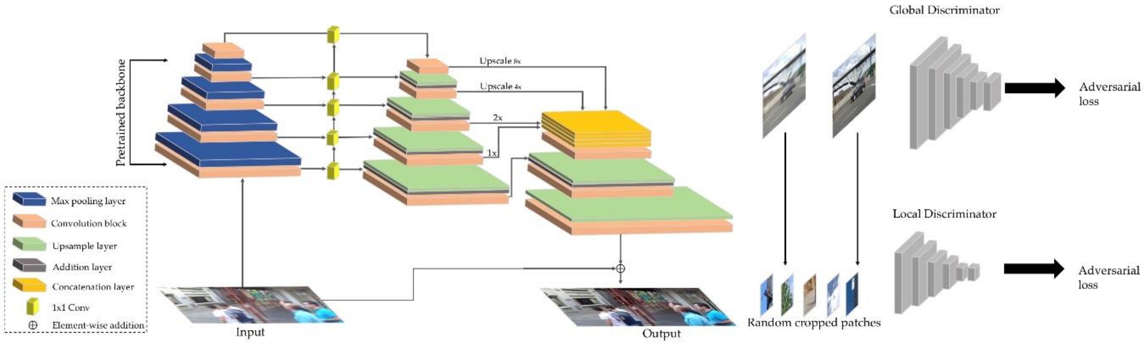
For the purposes of the study, a network model (Figure 1) was implemented in a PyTorch environment [89]. The network training was conducted using a Tryton supercomputer (computing power of 1.5 PFLOPS, 1600 computing nodes, 218 TB RAM) of the Academic Computer Centre in Gdańsk. Next, the model was launched on a computer with a GeForce GTX 1060 graphics processor (GPU) and an CPU Intel(R) Core i7-7700K 4.20GHz processor.
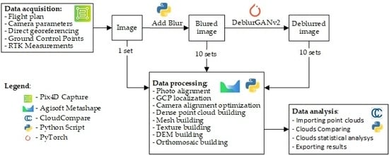
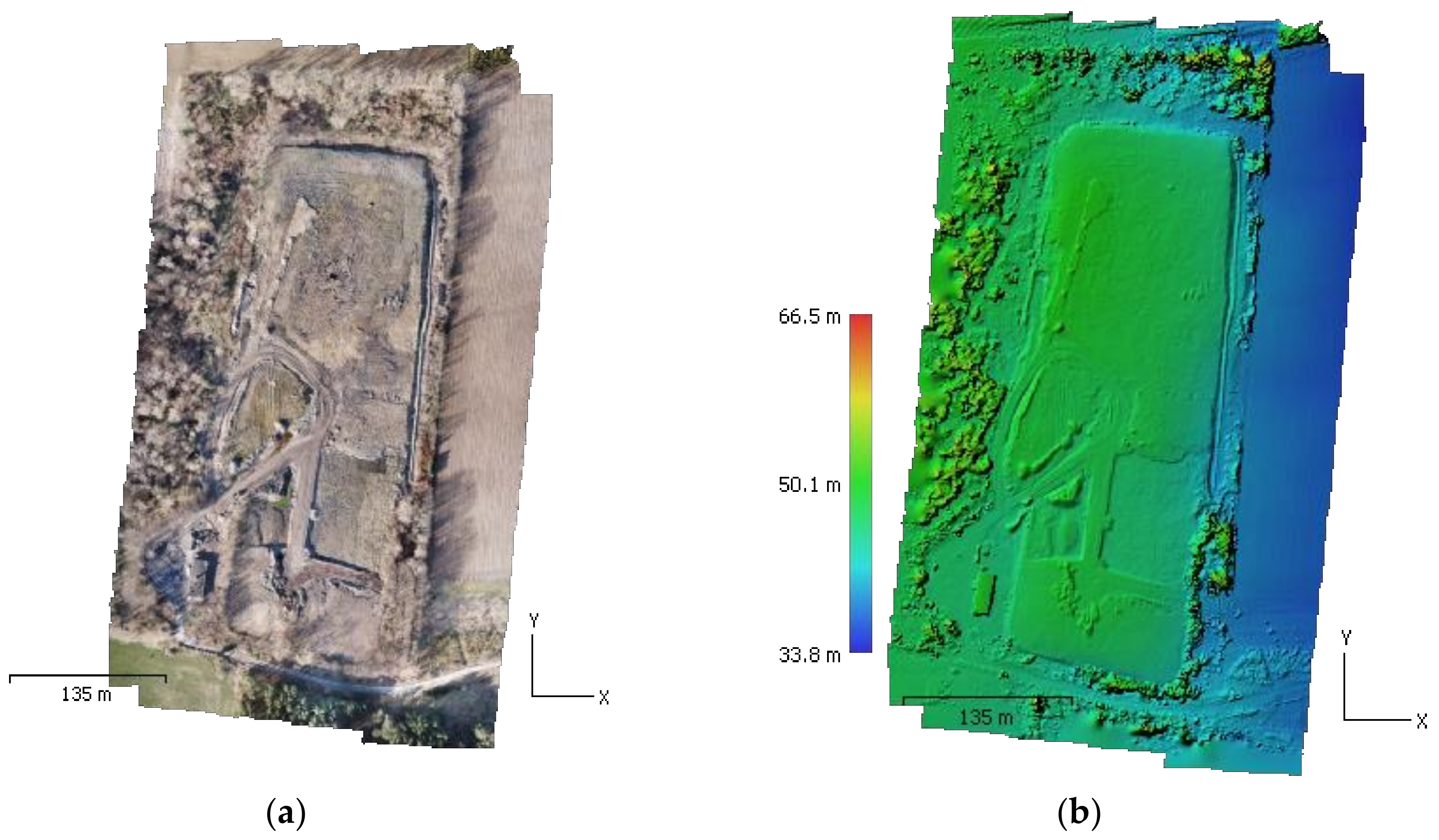
In order to verify the thesis of this paper, a test schedule and computation process were developed. The computation process in graphic form, together with used tools is shown in Figure 2. The test data were acquired using a commercial UAV. Models generated based on the data were adopted as reference models. The next stage is adding blur to the photos. A total of 10 sets of photos with a varying, increasing blur kernel were generated, and then used to generate 10 photogrammetric models. Next, all sets with blur were subject to the DeblurGANv2 method, which consequently enabled us to generate 10 new sets of image data, once again used to develop 10 photogrammetric models, using the same processing settings, as in previous cases. The details of these operations are shown in the further section of this paper.
2.2. Data Acquisition
The photogrammetric flight was conducted using a DJI Mavic Pro (Shenzhen DJI Sciences and Technologies Ltd., China) UAV. Such an unmanned aerial vehicle is a representative of commercial aerial vehicles, designed and intended primarily for recreational flying and for amateur movie-makers. The versatility and reliability of these devices was quickly appreciated by the photogrammetric community. Their popularity results mainly from the operational simplicity and intuitive software [28,66,90].
The flight was programmed and performed as per a single grid plan [91] over a landfill being reclaimed. The progress of the work in this area is periodically monitored using photogrammetry and terrestrial laser scanning. The dimensions of the test area are 240 × 505 m, with the flight conducted at an altitude of 80 m AGL, with a longitudinal and transverse overlap of 75%. A total of 224 photos were taken and marked with an actual UAV position. The UAV position is saved in the EXIF metadata (Exchangeable Image File Format). In addition, the photogrammetric network was developed. Six ground control points (GCPs) were evenly arranged throughout the entire study area, and their position was measured with the GNSS RTK accurate satellite positioning method. GCP position was determined relative to the PL-2000 Polish flat coordinate system and their altitude relative to the quasigeoid. Commercial Agisoft Metashape ver. 1.6.2 (Agisoft LLC, Russia) software was used to process the image data.
2.3. Blurred Data Set
A data set was developed for the GAN model training. The data set contains images acquired using the UAV. All images used were collected during many previous studies conducted by the author. The images mainly represent different types of terrain covered with vegetation and city areas, which were designed to develop typical photogrammetric models. The data set consists of two groups, namely images used for training and images used for trained model verification. These are different photos, which are not present in any of the two groups. The images used to train the neural network cannot be used to validate the trained model. Image pairs, sharp and with added random blur, were generated in each group.
The blur algorithm was implemented in the Python environment, using an OpenCV library [92], according to the following relationship:
where: represents a resulting image with a size of , represents a 2D discrete convolution function, and the source image with the dimensions of is described in the form of . It was assumed that , whereas the values of a 2D function for line take the values of , with the remaining ones taking 0.
The aforementioned relationships were used to generate both training data, as well as research data. Image data acquired during a reference flight were blurred. A total of 10 sets of research data, with a varying, increasing blur, were generated. The blur was changed by changing the blur kernel K size and adopting a uniform K for each research set.
Next, the same process of generating typical low-ceiling photogrammetry products was conducted using the photogrammetric software. This process followed the same procedure and processing settings as the ones applied for generating reference products. The result was 10 products generated from images with blur. Table 2 presents basic data of the surveys with data subject to blurring. It should be noted that a real flight altitude (75 m) was fixed, and the one shown in the table was calculated by the software. Table 3 shows a mean camera location error, and Table 4 shows the root mean square error (RMSE) calculated for control point locations. In the course of the photo processing process, the control points were manually indicated by the operator for each data set. The points were marked until the moment, when it was impossible to recognize them in the photos and possible to mark their center or the probable GCP center. The fact that it was possible to develop models from all data with blur, and that the software selected for this task completed the process without significant disturbance is noteworthy.
The measurement performed by an on-board GPS records the position and altitude relative to the WGS84 ellipsoid. The GCP position was determined relative to the Polish PL-2000 flat coordinate system and the altitude relative to PL-EVRF2007-NH quasigeoid. As presented in Table 3, the error values for the sharp data set (kernel value 0) in the horizontal plane (x,y) are within the range typical for GPS receivers used in commercial UAVs. The absolute error in the vertical plane (z) is significantly greater and results directly from using different altitude reference systems. Total error for camera location correlates with total RMSE presented in Table 4. The GPS remains unchanged during the flight and it should be assumed that the position accuracy is relatively constant throughout the flight. The total camera location error relates to the positions of the measured control points, the accuracy of which decreases significantly above kernel value 20, and should not be considered as valid.
The control points were manually marked by the operator and up to blur kernel 20 it was possible to mark all 6 points. In a normal case, in terms of practical work, a number of 6 GCPs is the lowest reasonable number to achieve satisfactory results. Up to kernel 20, the total RMSE is growing with maximum at a blur kernel equal to 20. For a blur kernel greater than 20, some of the points were not sharp and visible enough and were not considered as correct ones and not marked in the software. Consequently, errors were calculated for a smaller number of GCPs, and total RMSE values for a blur kernel > 20 is lower that values for all 6 points marked on kernel 20. Generally, using 4 or 3 GPSs may induce errors for the final results and is not recommended in the practical cases. Despite the fact that total RMSE for a blur kernel > 20 could be satisfactory, the number of marked GCPs is too low and should be treated as a non-representative GCP’s error result and not used in the practical cases. Practically, results represented in total RMSE are satisfactory for a blur kernel up to 10, where the operator was able to mark all GCPs and total RMSE at around 2 cm.
2.4. Deblurring with GAN
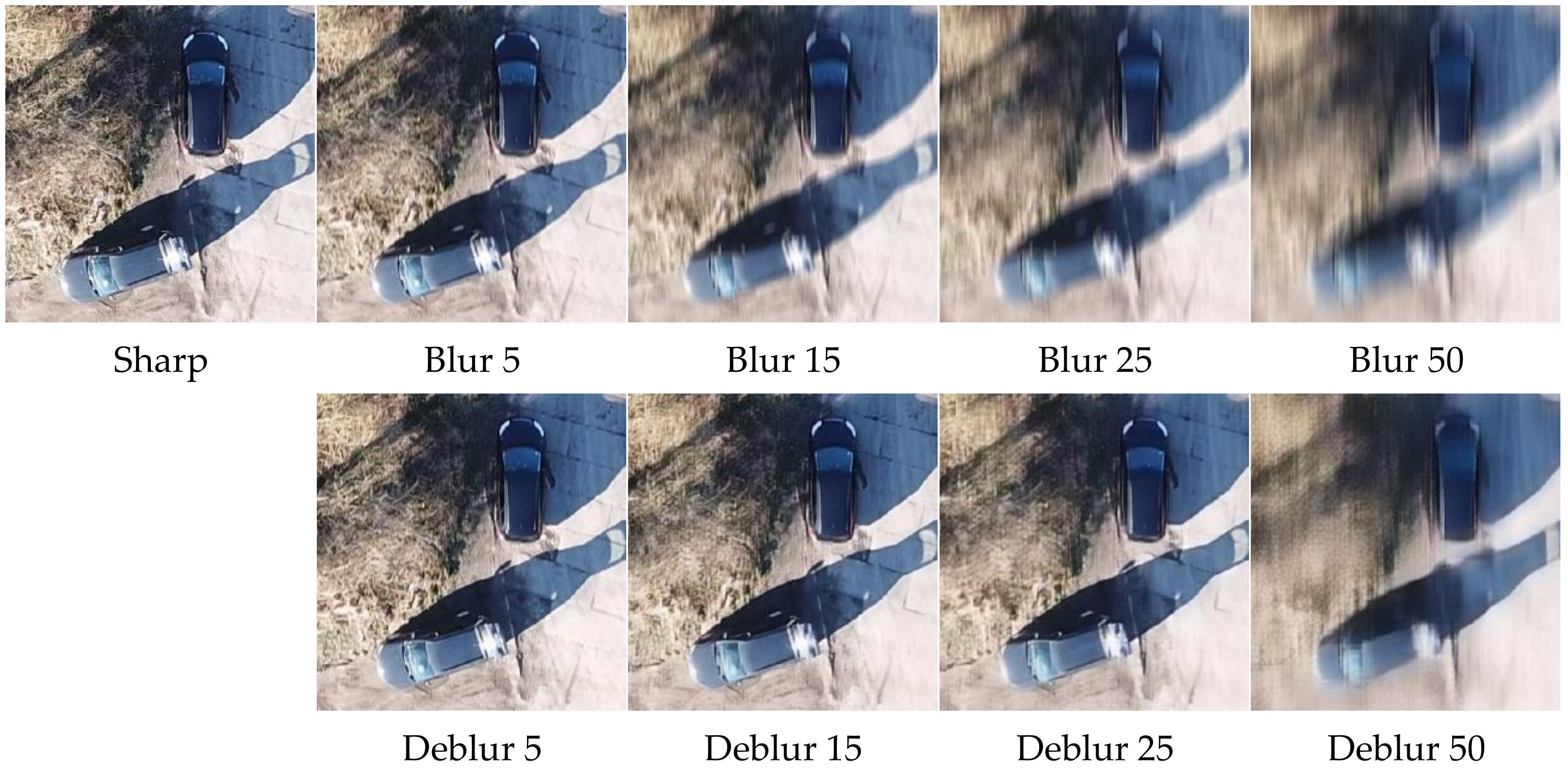
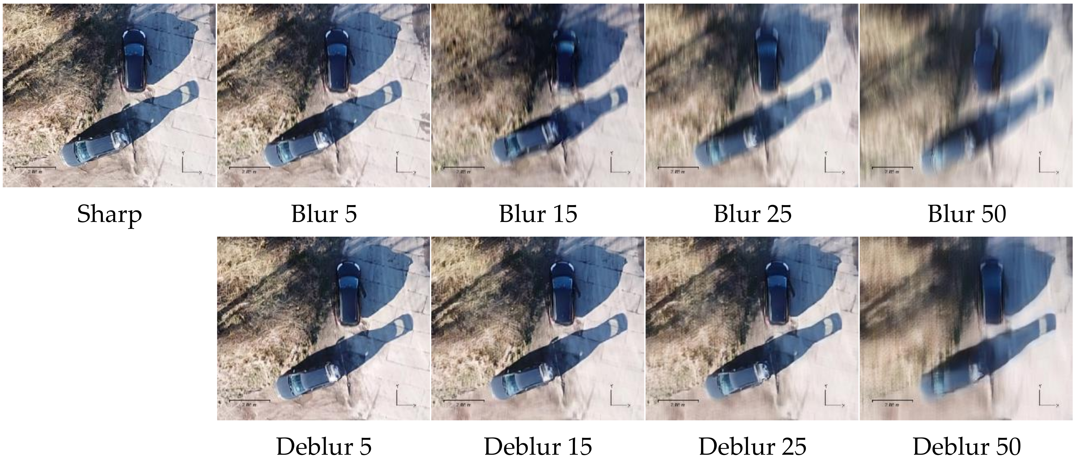
All sets with applied blur were individually subjected to the deblurring process. For this purpose, images with blur were successively provided as input data for a trained generative adversarial network model. The resulting images for each set were used to generate ten further sets of photogrammetric products. This process was similar to the one involving reference models, with the same processing software settings being used. Figure 4 shows a visual comparison of the results for the DebluGANv2 algorithm for GCP No. 1. The images show, respectively, a reference photo (sharp), photos with blur for kernel 5, 15, 25 and 50, and the corresponding images with blur reduction.
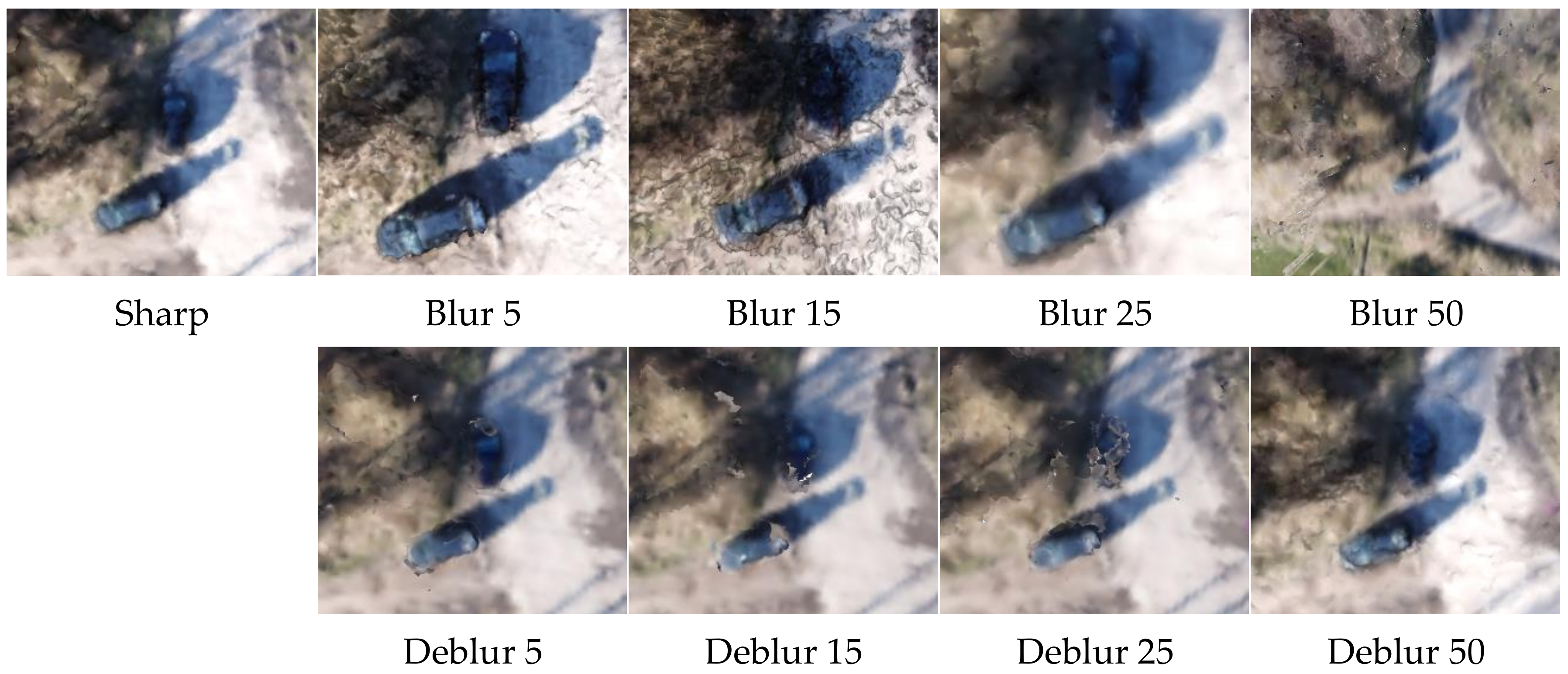
A visual analysis of the images indicates that this image significantly reduces blur to a level of K = 25. This method is particularly effective with sharp and clear edges, lines generated by anthropogenic structures, such as buildings, borders between various ground surfaces, cars, sharp shadows, etc. This phenomenon enables a visual improvement in the recognizability of ground control points and other objects of artificial (anthropogenic) origin (Figure 5). Control point edges in images with blur are clearly blurred, which hinders its proper indication in a photogrammetric program. In practice, it becomes very difficult with a blur kernel above 15. A significant improvement in the sharpness of the control point edge can be noticed in photos subjected to deblurring. When it comes to the control point, this phenomenon improves its recognizability in a terrain and enables its more accurate indication in a photogrammetric program.
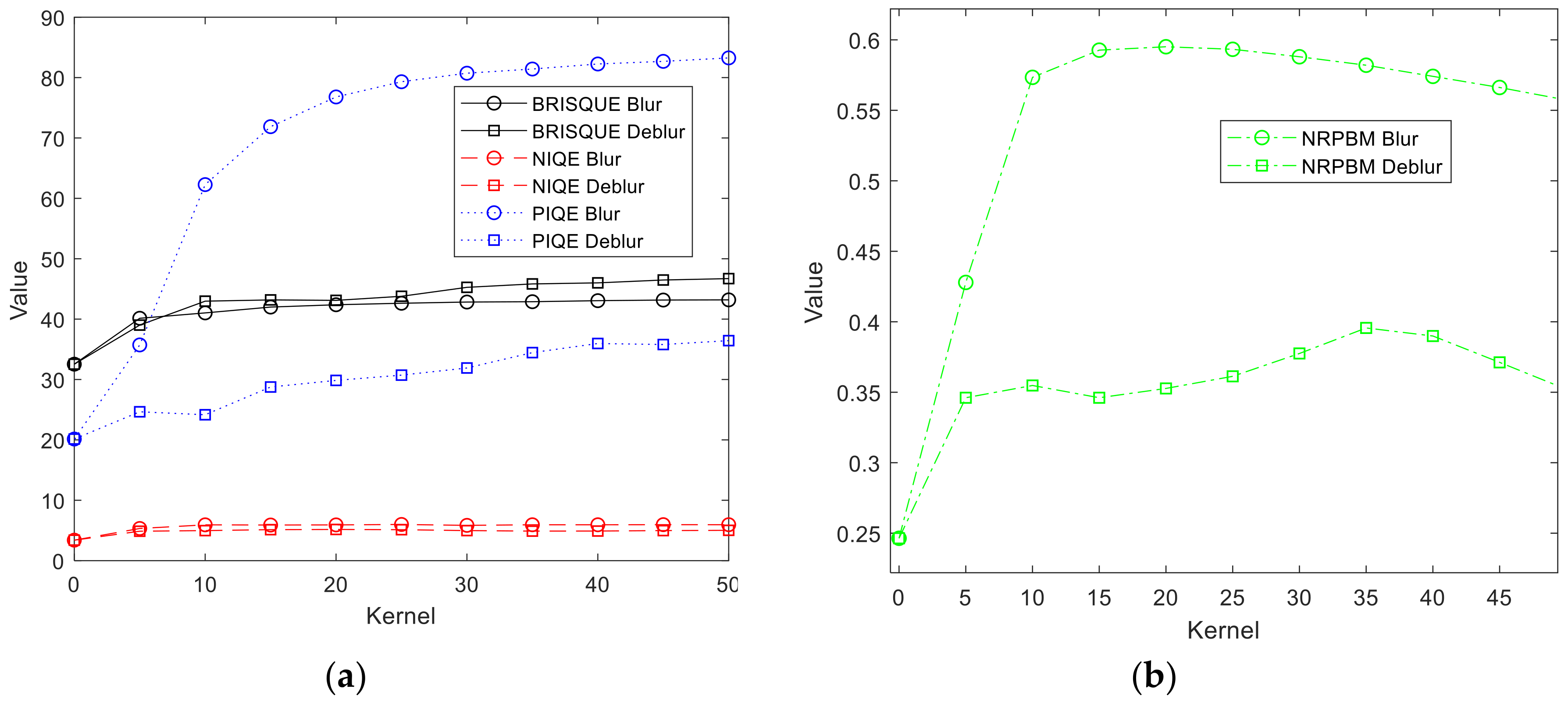
The assessment of image qualities and the evaluation of the DeblurGANv2 method in comparison with the blurred images was conducted on the basis of three different image quality metrics (IQMs): blind referenceless image spatial quality evaluator (BRISQUE) [93], natural image quality evaluator (NIQE) [94], perception-based image quality evaluator (PIQE) [95] and no-reference perceptual blur metric (NRPBM) [96]. Chosen no-reference image quality scores generally return a non-negative scalar. The BRISQUE score is in the range from 0 to 100. Lower score values better reflect perceptive qualities of images. The NIQE model is trained on a database of pristine images and can measure the quality of images with arbitrary distortion. The NIQE is opinion unaware and does not use subjective quality scores. The trade-off is that the NIQE score of an image might not correlate as well as the BRISQUE score with human perceptions of quality. Lower score values better reflect the perceptive qualities of images with respect to the input model. The PIQE score is the no-reference image quality score, and it is inversely correlated to the perceptual quality of an image. A low score value indicates high perceptive quality, and high-score values indicates low perceptive quality. The NRPBM is ranging from 0 to 1, which are, respectively, the best and the worst quality in terms of blur perception. Table 5 shows calculated results of the aforementioned image quality evaluators. Figure 6 presents quality evaluation in graphical form.
The analysis of the results shown in Figure 6 emphasizes a clear improvement in image quality after the application of this method. The PIQE and NRPBM indices recorded a particularly significant improvement. The PIQE index correlates with the image perception by humans. Therefore, the visual, subjective image quality improvement presented in Figure 5 was confirmed by the PIQE index. The NRPBM index, especially intended for an objective blur evaluation in images, clearly points to a significant improvement in the quality for all data sets, with the greatest improvement for K = 15 and K = 20.
Photos subjected to the DeblurGANv2 method were used as a base to develop successive, typical photogrammetric products. This process followed the same procedure and processing settings, as the ones applied for generating reference products and photos with blur. The result was 10 products generated using synthetic photos, generated by neural networks. Table 6 presents basic study data based on photos without blurring. Table 7 shows a mean camera location error, and Table 8 the RMSE calculated for control point location. In this case, the points were also marked until the moment, when it was impossible to recognize them in the photos and possible to mark their center or the probable GCP center. It should be stressed that the operator was able to indicate all six control points for each blur kernel. They were possible to find and identify on all data sets.
Figure 7 graphically presents a comparison of all reported survey data for blurred and deblurred data set. The subfigures are presented in the following order: the number of tie points, the number of projections, reprojection errors, camera location total error, GCP total RMSE and the number of marked GCPs.
3. Results
This chapter presents and analyzes photogrammetric products developed both using blurred photos, as well as their corresponding deblurred photos. Figure 8 shows a fragment of a developed textured surface model. It should be noted that the texture was generated in each case, and it covered the surface model (mesh) in the right place. The texture quality is responsible for the quality of source photos. The blur visible in the photos is also visible on the surface model. As with the photos themselves, a clear mapping of the borders between sharp edges can be observed. The texture of anthropogenic models is clear, and a significant visual improvement was recorded in this regard. Such conclusions can also be directly derived from the parametric evaluation of the photos in Figure 6.
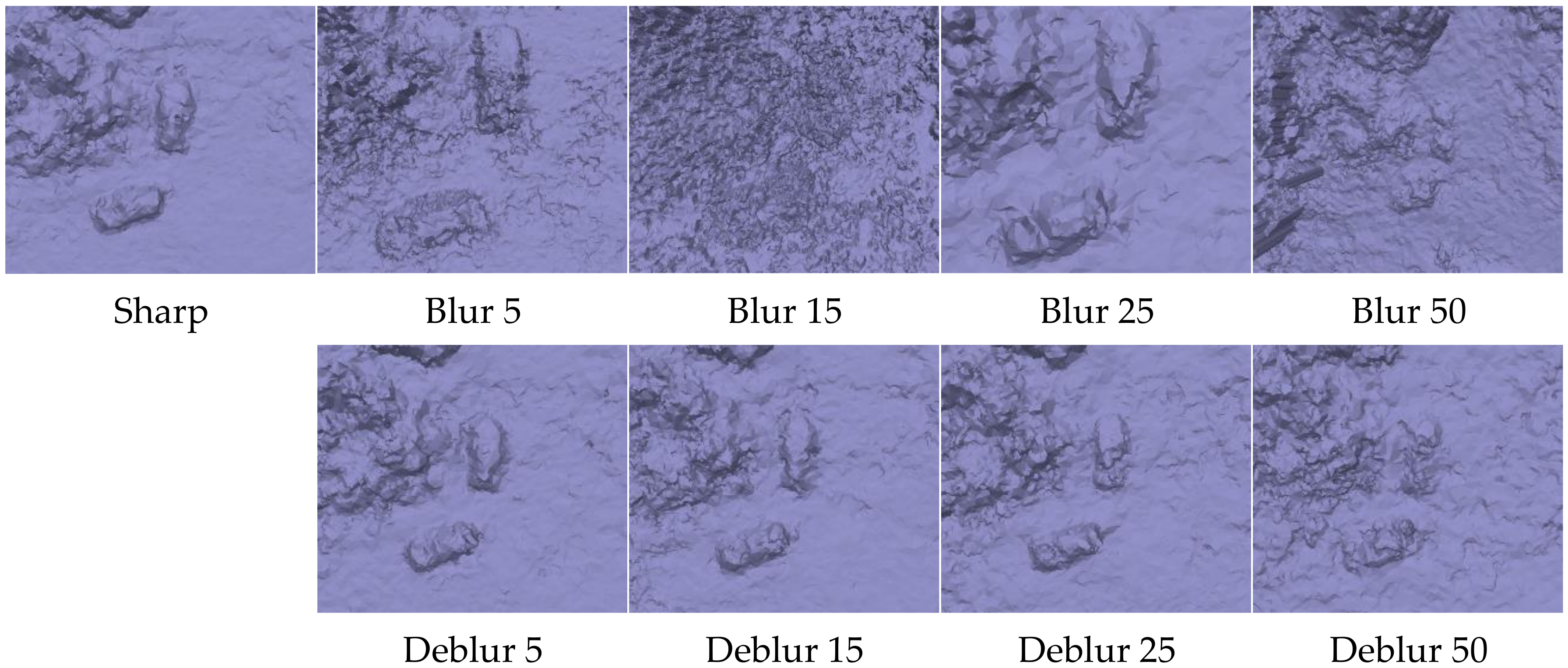
A textured digital surface model does not enable visually assessing the model geometric quality. For this purpose, Figure 9 shows a digital surface model in a uniform color. First of all, it should be noted that the terrain surface was mapped with geometry in models developed using photos without blur. Cars visible in this fragment have clearly marked edges. In the case of a blurred model, one can notice a lack of model generating correlation and stability, along with a blur kernel increase. For K = 15 and K = 50, the models of smaller objects on the surface are not mapped in practice.
As stated earlier, a significantly improved human perception of the photos is achieved. This allows us to conclude that the interpretive quality of an orthoimage generated using such photos will correlate with the quality of source photographs. Figure 10 shows fragments of developed orthophotomaps. A clear improvement in the interpretive quality of such a product can be observed in such images. Significantly blurred objects, e.g., due to their motion, are much clearer on an orthophotomap. This proves that enhancing source photos with the DeblurGANv2 methods translated directly to improving the interpretive quality of an orthophotomap.
The geometric quality of developed relief models was evaluated using the methods described in [30,97]. An M3C2 distance map (Multiscale Model to Model Cloud Comparison) was developed for each point cloud. The M3C2 distance map computation process utilized 3-D point precision estimates stored in scalar fields. Appropriate scalar fields were selected for both point clouds (referenced and tested) to describe measurement precision in X, Y and Z (sigmaX, sigmaY and sigmaZ). The results for sample blurs are shown in Figure 11. As can be seen in the presented images, in the case of models based on photos without blur, the distance of a tested model to a reference cloud is stable and there are no significant differences, which is depicted by an even green color over the entire area. In the case of images with blur, as might have been expected, the geometry of the entire surface has been significantly modified. Model deformation, resulting from the systemic errors occurring during aerotriangulation (so-called doming error), increases together with an increasing blur kernel and adopts values of up to 50 m, at the boundaries of the modelled surface.
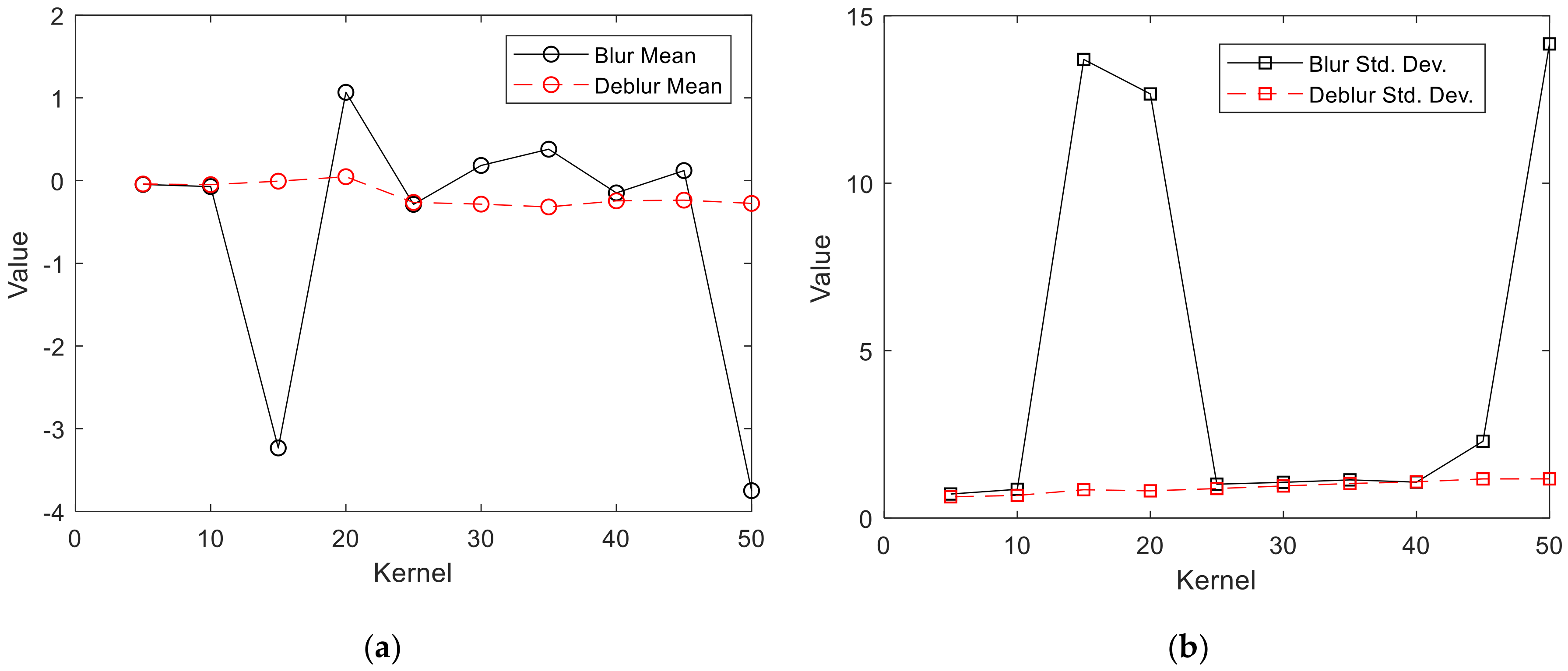
The statistical evaluation of calculated M3C2 distances for all variants was shown in Table 9 and its graphic form in Figure 12. The statistical distribution of M3C2 distances is close to normal, which means that a significant part of the observations is concentrated around the mean. The mean and standard deviations for blurred images are not stable and change drastically depending on the blur kernel. The drastic change is observed for 15, 20 and 50 kernels. High stability can be observed for models generated from deblurred photos. The mean varies around zero and the standard deviation grows steadily, to take twice the initial value for the highest blur kernel.
4. Conclusions
The results presented in the previous section show that the method for improving blurred photo quality significantly contributed to an improvement in the general quality of typical photogrammetric products. The model quality can be analyzed in terms of their geometric accuracy and interpretive quality.
The geometric accuracy of the models generated from photos without blur was maintained, which is evidenced by the low means and standard deviation of the compared models. This deviation steadily increases with a growing blur kernel. There was also no significant doming error in these models, which leads to the correct generation of a digital surface model, which preserves severe altitude changes in object edges. As has been shown, object edges in blurred photos fade away at higher blur kernel values. The proposed method enables emphasizing these edges, which consequently retain their geometry.
The interpretive quality of textured products and photos clearly increased. It has been shown, beyond any doubt, that blur reduction significantly improves image perception, and the objects depicted in an orthoimage are clearer. According to the author, this property has great potential for practical application, especially for the reconstruction of highly urbanized places and objects. Blur reduction was higher in image areas with strongly marked non-natural objects (buildings, roads, cars, etc.). This fact largely results from the nature of the photos used for neural network model training. The majority were photos showing fragments of urbanized areas. This property strongly improves the interpretive properties and can be used to develop the maps of urban areas, as well as to extract land cover elements from an orthophotomap.
In the case of the used GCPs (plate with a 30 cm × 30 cm graphic symbol), it was possible to indicate them, even in photos with an initially highest blur. It certainly improved the aerotriangulation outcome and the geometry of the developed models. However, the visibility of these points was not fully maintained, which can constitute grounds to further research of this method. At this point, one can lay a hypothesis that by training networks using photos of similar GCPs or an image of typical GCPs used in photogrammetry, it is possible to enhance and obtain a significant improvement in blur reduction in images showing ground, signaled control points.
The method for improving the quality of blurred photos applied in this research paper has been tested using typical photogrammetric software. Surprisingly, the software turned out to be rather blur resistant and enabled generating models based on all test data, even the ones with the highest blur. It is a fact that the surface of the modelled terrain was deformed; nevertheless, the course of the process of developing a model based on blurred photos was typical. Both the geometric, as well as the interpretive quality of developed photogrammetric models were improved using the neural method for reducing blur, based on generative adversarial networks.
In the conventional photogrammetric process, blurred images are completely unusable. In specific cases, it may turn out that all images have visible blur for the entire photogrammetric flight. This situation means that it is very difficult to locate GCPs, object details and edges are unclear and fading, and images have a weak interpretation quality. The application of the method will eliminate any blurred images and, consequently, it will be possible to use the acquired data for the modelling. In photogrammetric software, which is commonly employed and particularly in their cloud versions, it will be possible to implement an additional feature, which will eliminate unwanted blur. The performance of the method based on neural networks is relatively fast, which means that its application will not significantly slow down the process of building photogrammetric models. Additionally, the application of the method significantly expands the capabilities of the photogrammetric software, due to its universality and independence from the blur character.
Funding
This research received no external funding
Acknowledgments
Calculations were carried out at the Academic Computer Centre in Gdansk.
Conflicts of Interest
The authors declare no conflict of interest.
References
- Specht, C.; Mania, M.; Skóra, M.; Specht, M. Accuracy of the GPS Positioning System in the Context of Increasing the Number of Satellites in the Constellation. Pol. Marit. Res. 2015. [Google Scholar] [CrossRef] [Green Version]
- Burdziakowski, P.P.; Bobkowska, K. Accuracy of a Low-cost Autonomous Hexacopter Platforms Navigation Module for a Photogrammetric and Environmental Measurements. In Proceedings of the 10th International Conference “Environmental Engineering”, VGTU Technika, Vilnius, Lithuania, 27–28 April 2017. [Google Scholar]
- Specht, C.; Pawelski, J.; Smolarek, L.; Specht, M.; Dabrowski, P. Assessment of the Positioning Accuracy of DGPS and EGNOS Systems in the Bay of Gdansk using Maritime Dynamic Measurements. J. Navig. 2019. [Google Scholar] [CrossRef] [Green Version]
- Hugenholtz, C.; Brown, O.; Walker, J.; Barchyn, T.; Nesbit, P.; Kucharczyk, M.; Myshak, S. Spatial Accuracy of UAV-Derived Orthoimagery and Topography: Comparing Photogrammetric Models Processed with Direct Geo-Referencing and Ground Control Points. Geomatica 2016, 70, 21–30. [Google Scholar] [CrossRef]
- Zimmermann, F.; Eling, C.; Klingbeil, L.; Kuhlmann, H.J. Precise positioning of uavs–dealing with challenging rtk-gps measurement conditions during automated uav flights. ISPRS Ann. Photogramm. Remote Sens. Spat. Inf. Sci. 2017, IV-2/W3, 95–102. [Google Scholar] [CrossRef] [Green Version]
- Roosevelt, C.H. Mapping site-level microtopography with Real-Time Kinematic Global Navigation Satellite Systems (RTK GNSS) and Unmanned Aerial Vehicle Photogrammetry (UAVP). Open Archaeol. 2014, 1. [Google Scholar] [CrossRef]
- Tahar, K.N.; Ahmad, A.; Akib, W.A.A.W.M.; Mohd, W.M.N.W. Unmanned Aerial Vehicle Photogrammetric Results Using Different Real Time Kinematic Global Positioning System Approaches; Abdul Rahman, A., Boguslawski, P., Gold, C., Said, M.N., Eds.; Springer: Berlin/Heidelberg, Germany, 2013; pp. 123–134. ISBN 978-3-642-36379-5. [Google Scholar]
- Chao, H.; Coopmans, C.; Di, L.; Chen, Y. A comparative evaluation of low-cost IMUs for unmanned autonomous systems. In Proceedings of the 2010 IEEE Conference on Multisensor Fusion and Integration, Salt Lake City, UT, USA, 5–7 September 2010; pp. 211–216. [Google Scholar]
- Hartley, R.; Zisserman, A. Multiple View Geometry in Computer Vision; Cambridge University Press: Cambridge, UK, 2004. [Google Scholar]
- Dai, F.; Feng, Y.; Hough, R. Photogrammetric error sources and impacts on modeling and surveying in construction engineering applications. Vis. Eng. 2014, 2, 2. [Google Scholar] [CrossRef] [Green Version]
- Wierzbicki, D.; Kedzierski, M.; Fryskowska, A.; Jasinski, J. Quality Assessment of the Bidirectional Reflectance Distribution Function for NIR Imagery Sequences from UAV. Remote Sens. 2018, 10, 1348. [Google Scholar] [CrossRef] [Green Version]
- Kedzierski, M.; Delis, P. Fast orientation of video images of buildings acquired from a UAV without stabilization. Sensors 2016. [Google Scholar] [CrossRef]
- Wierzbicki, D.; Kedzierski, M.; Sekrecka, A. A Method for Dehazing Images Obtained from Low Altitudes during High-Pressure Fronts. Remote Sens. 2019, 12, 25. [Google Scholar] [CrossRef] [Green Version]
- Sekrecka, A.; Kedzierski, M.; Wierzbicki, D. Pre-Processing of Panchromatic Images to Improve Object Detection in Pansharpened Images. Sensors 2019, 19, 5146. [Google Scholar] [CrossRef] [Green Version]
- Sekrecka, A.; Wierzbicki, D.; Kedzierski, M. Influence of the Sun Position and Platform Orientation on the Quality of Imagery Obtained from Unmanned Aerial Vehicles. Remote Sens. 2020, 12, 1040. [Google Scholar] [CrossRef] [Green Version]
- Calì, M.; Oliveri, S.M.; Fatuzzo, G.; Sequenzia, G. Error control in UAV image acquisitions for 3D reconstruction of extensive architectures. In Lecture Notes in Mechanical Engineering; Springer: Cham, Switzerland, 2017. [Google Scholar] [CrossRef]
- Kedzierski, M.; Wierzbicki, D. Radiometric quality assessment of images acquired by UAV’s in various lighting and weather conditions. Measurement 2015, 76, 156–169. [Google Scholar] [CrossRef]
- Kedzierski, M.; Wierzbicki, D. Methodology of improvement of radiometric quality of images acquired from low altitudes. Meas. J. Int. Meas. Confed. 2016. [Google Scholar] [CrossRef]
- Kedzierski, M.; Wierzbicki, D.; Sekrecka, A.; Fryskowska, A.; Walczykowski, P.; Siewert, J. Influence of Lower Atmosphere on the Radiometric Quality of Unmanned Aerial Vehicle Imagery. Remote Sens. 2019, 11, 1214. [Google Scholar] [CrossRef] [Green Version]
- Haala, N.; Cramer, M.; Rothermel, M. Quality of 3D point clouds from highly overlapping UAV imagery. Int. Arch. Photogramm. Remote Sens. Spat. Inf. Sci. 2013, XL-1/W2, 183–188. [Google Scholar] [CrossRef] [Green Version]
- Nocerino, E.; Menna, F.; Remondino, F.; Saleri, R. Accuracy and block deformation analysis in automatic UAV and terrestrial photogrammetry-Lesson learnt. ISPRS Ann. Photogramm. Remote Sens. Spat. Inf. Sci. 2013, 2, 203–208. [Google Scholar] [CrossRef] [Green Version]
- Kršák, B.; Blišťan, P.; Pauliková, A.; Puškárová, P.; Kovanič, L.; Palková, J.; Zelizňaková, V. Use of low-cost UAV photogrammetry to analyze the accuracy of a digital elevation model in a case study. Meas. J. Int. Meas. Confed. 2016. [Google Scholar] [CrossRef]
- Burdziakowski, P.; Tysiac, P. Combined Close Range Photogrammetry and Terrestrial Laser Scanning for Ship Hull Modelling. Geosciences 2019, 9, 242. [Google Scholar] [CrossRef] [Green Version]
- Bakuła, K.; Ostrowski, W.; Pilarska, M.; Szender, M.; Kurczyński, Z. Evaluation and calibration of fixed-wing UAV mobile mapping system equipped with LiDar and optical sensors. Int. Arch. Photogramm. Remote Sens. Spat. Inf. Sci. 2018, XLII-1, 25–32. [Google Scholar] [CrossRef] [Green Version]
- Oktay, T.; Celik, H.; Turkmen, I. Maximizing autonomous performance of fixed-wing unmanned aerial vehicle to reduce motion blur in taken images. Proc. Inst. Mech. Eng. Part I J. Syst. Control Eng. 2018, 232, 857–868. [Google Scholar] [CrossRef]
- Hamledari, H.; McCabe, B.; Davari, S.; Shahi, A.; Rezazadeh Azar, E.; Flager, F. Evaluation of computer vision-and 4D BIM-based construction progress tracking on a UAV platform. In Proceedings of the 6th Csce/Asce/Crc International Construction Specialty Conference, Vancouver, BC, Canada, 31 May–3 June 2017. [Google Scholar]
- Markiewicz, J.; Łapiński, S.; Kot, P.; Tobiasz, A.; Muradov, M.; Nikel, J.; Shaw, A.; Al-Shamma’a, A. The Quality Assessment of Different Geolocalisation Methods for a Sensor System to Monitor Structural Health of Monumental Objects. Sensors 2020, 20, 2915. [Google Scholar] [CrossRef] [PubMed]
- Burdziakowski, P. Increasing the Geometrical and Interpretation Quality of Unmanned Aerial Vehicle Photogrammetry Products using Super-Resolution Algorithms. Remote Sens. 2020, 12, 810. [Google Scholar] [CrossRef] [Green Version]
- Hastedt, H.; Luhmann, T. Investigations on the quality of the interior orientation and its impact in object space for UAV photogrammetry. International Archives of the Photogrammetry. Remote Sens. Spat. Inf. Sci. 2015, 40. [Google Scholar]
- James, M.R.; Robson, S.; D’Oleire-Oltmanns, S.; Niethammer, U. Optimising UAV topographic surveys processed with structure-from-motion: Ground control quality, quantity and bundle adjustment. Geomorphology 2017, 280, 51–66. [Google Scholar] [CrossRef] [Green Version]
- Markiewicz, J.; Zawieska, D. Analysis of the Selection Impact of 2D Detectors on the Accuracy of Image-Based TLS Data Registration of Objects of Cultural Heritage and Interiors of Public Utilities. Sensors 2020, 20, 3277. [Google Scholar] [CrossRef] [PubMed]
- Dominik, W.A. Exploiting the Redundancy of Multiple Overlapping Aerial Images for Dense Image Matching Based Digital Surface Model Generation. Remote Sens. 2017, 9, 490. [Google Scholar] [CrossRef] [Green Version]
- Pacey, R.; Fricker, P. Forward motion compensation (FMC)-is it the same in the digital imaging world? Photogramm. Eng. Remote Sens. 2005, 71, 1241–1242. [Google Scholar]
- Cox, R.C.A. The benefits of forward motion compensation for aerial survey photography. Photogramm. Rec. 2006, 14, 5–17. [Google Scholar] [CrossRef]
- Pain, B.; Cunningham, T.J.; Yang, G.; Ortiz, M. Time-Delayed-Integration Imaging with Active Pixel Sensors. U.S. Patent No. 7,268,814, 11 September 2007. [Google Scholar]
- Lepage, G. Time Delayed Integration CMOS Image Sensor with Zero Desynchronization. U.S. Patent No. 7,675,561, 9 March 2010. [Google Scholar]
- Lepage, G.; Bogaerts, J.; Meynants, G. Time-Delay-Integration Architectures in CMOS Image Sensors. IEEE Trans. Electron Devices 2009, 56, 2524–2533. [Google Scholar] [CrossRef]
- Wong, H.-S.; Yao, Y.L.; Schlig, E.S. TDI charge-coupled devices: Design and applications. IBM J. Res. Dev. 1992, 36, 83–106. [Google Scholar] [CrossRef]
- Tang, X.; Hu, F.; Wang, M.; Pan, J.; Jin, S.; Lu, G. Inner FoV Stitching of Spaceborne TDI CCD Images Based on Sensor Geometry and Projection Plane in Object Space. Remote Sens. 2014, 6, 6386–6406. [Google Scholar] [CrossRef] [Green Version]
- Chabok, M. Eliminating and modelling non-metric camera sensor distortions Caused by sidewise and forward motion of the UAV. Int. Arch. Photogramm. Remote Sens. Spat. Inf. Sci. 2013, 40, 73–79. [Google Scholar]
- Sieberth, T.; Wackrow, R.; Chandler, J.H. Influence of blur on feature matching and a geometric approach for photogrammetric deblurring. Int. Arch. Photogramm. Remote Sens. Spat. Inf. Sci. 2014, XL-3, 321–326. [Google Scholar] [CrossRef] [Green Version]
- Sieberth, T.; Wackrow, R.; Chandler, J.H. UAV image blur-Its influence and ways to correct it. Int. Arch. Photogramm. Remote Sens. Spat. Inf. Sci. 2015, 40, 33. [Google Scholar] [CrossRef] [Green Version]
- Lu, W.; Tong, L.; Li, M.; Li, C. Parameters optimization in blind motion deblurring of UAV images. In Proceedings of the Fifth International Conference on Computing, Communications and Networking Technologies (ICCCNT), Hefei, China, 11–13 July 2014; pp. 1–5. [Google Scholar] [CrossRef]
- Hammer, A.; Dumoulin, J.; Vozel, B.; Chehdi, K. Deblurring of UAV aerial images for civil structures inspections using Mumford-Shah/Total variation regularisation. In Proceedings of the 2007 5th International Symposium on Image and Signal Processing and Analysis, Istanbul, Turkey, 27–29 September 2007; pp. 262–267. [Google Scholar]
- Lelégard, L.; Delaygue, E.; Brédif, M.; Vallet, B. Detecting and correcting motion blur from images shot with channel-dependent exposure time. ISPRS Ann. Photogramm. Remote Sens. Spat. Inf. Sci. 2012, 1, 341–346. [Google Scholar]
- Du, Y.; Liu, N.; Xu, Y.; Liu, R. Deblurring Crack Images Generated by UAV Camera Shake. In Proceedings of the 2017 IEEE 7th Annual International Conference on CYBER Technology in Automation, Control, and Intelligent Systems (CYBER), Hawaii, HI, USA, 31 July–4 August 2017; pp. 175–178. [Google Scholar]
- Koik, B.T.; Ibrahim, H. Exploration of Current Trend on Blur Detection Method Utilized in Digital Image Processing. J. Ind. Intell. Inf. 2013, 1, 143–147. [Google Scholar] [CrossRef]
- Teo, T.-A.; Zhan, K.-Z. Integration of image-derived and pos-derived features for image blur detection. Int. Arch. Photogramm. Remote Sens. Spat. Inf. Sci. 2016, 41, 1051. [Google Scholar] [CrossRef]
- Jiang, W.; Zhang, D.; Yu, H. Sensor-assisted image deblurring of consumer photos on smartphones. In Proceedings of the 2014 IEEE International Conference on Multimedia and Expo (ICME), Chengdu, China, 14–18 July 2014; pp. 1–6. [Google Scholar]
- Shao, W.-Z.; Liu, Y.-Y.; Ye, L.-Y.; Wang, L.-Q.; Ge, Q.; Bao, B.-K.; Li, H.-B. DeblurGAN+: Revisiting blind motion deblurring using conditional adversarial networks. Signal Process. 2020, 168, 107338. [Google Scholar] [CrossRef]
- Zhou, S.; Zhang, J.; Pan, J.; Zuo, W.; Xie, H.; Ren, J. Spatio-Temporal Filter Adaptive Network for Video Deblurring. In Proceedings of the 2019 IEEE/CVF International Conference on Computer Vision (ICCV), Seoul, Korea, 27–28 October 2019; pp. 2482–2491. [Google Scholar]
- Wang, X.; Chan, K.C.K.; Yu, K.; Dong, C.; Loy, C.C. EDVR: Video restoration with enhanced deformable convolutional networks. In Proceedings of the 2019 IEEE/CVF Conference on Computer Vision and Pattern Recognition Workshops (CVPRW), Long Beach, CA, USA, 16–21 June 2019; pp. 1954–1963. [Google Scholar]
- Chen, C.; Chen, Q.; Xu, J.; Koltun, V. Learning to See in the Dark. In Proceedings of the 2018 IEEE/CVF Conference on Computer Vision and Pattern Recognition, Salt Lake City, UT, USA, 18–23 June 2018; pp. 3291–3300. [Google Scholar]
- Liu, P.; Janai, J.; Pollefeys, M.; Sattler, T.; Geiger, A. Self-Supervised Linear Motion Deblurring. IEEE Robot. Autom. Lett. 2020, 5, 2475–2482. [Google Scholar] [CrossRef] [Green Version]
- Zhang, X.; Dong, H.; Hu, Z.; Lai, W.S.; Wang, F.; Yang, M.H. Gated fusion network for joint image deblurring and super-resolution. In Proceedings of the British Machine Vision Conference, Newcastle, UK, 3–6 September 2018. BMVC 2019. [Google Scholar]
- Kupyn, O.; Budzan, V.; Mykhailych, M.; Mishkin, D.; Matas, J. DeblurGAN: Blind Motion Deblurring Using Conditional Adversarial Networks. In Proceedings of the 2018 IEEE/CVF Conference on Computer Vision and Pattern Recognition, IEEE, Salt Lake City, UT, USA, 18–23 June 2018; pp. 8183–8192. [Google Scholar]
- Zhou, S.; Zhang, J.; Zuo, W.; Xie, H.; Pan, J.; Ren, J.S. DAVANet: Stereo Deblurring With View Aggregation. In Proceedings of the 2019 IEEE/CVF Conference on Computer Vision and Pattern Recognition (CVPR), IEEE, Long Beach, CA, USA, 16–21 June 2019; pp. 10988–10997. [Google Scholar]
- Zhang, J.; Pan, J.; Ren, J.; Song, Y.; Bao, L.; Lau, R.W.H.; Yang, M.-H. Dynamic Scene Deblurring Using Spatially Variant Recurrent Neural Networks. In Proceedings of the 2018 IEEE/CVF Conference on Computer Vision and Pattern Recognition, Salt Lake City, UT, USA, 18–22 June 2018; pp. 2521–2529. [Google Scholar]
- Nah, S.; Kim, T.H.; Lee, K.M. Deep Multi-scale Convolutional Neural Network for Dynamic Scene Deblurring. In Proceedings of the 2017 IEEE Conference on Computer Vision and Pattern Recognition (CVPR), Honolulu, HI, USA, 21–26 July 2017; pp. 257–265. [Google Scholar]
- Shen, Z.; Lai, W.-S.; Xu, T.; Kautz, J.; Yang, M.-H. Deep Semantic Face Deblurring. In Proceedings of the 2018 IEEE/CVF Conference on Computer Vision and Pattern Recognition, Salt Lake City, UT, USA, 18–22 June 2018; pp. 8260–8269. [Google Scholar]
- Zhang, K.; Zuo, W.; Zhang, L. Deep Plug-And-Play Super-Resolution for Arbitrary Blur Kernels. In Proceedings of the 2019 IEEE/CVF Conference on Computer Vision and Pattern Recognition (CVPR), Long Beach, CA, USA, 16–21 June 2019; pp. 1671–1681. [Google Scholar]
- Zhang, Y.; Tian, Y.; Kong, Y.; Zhong, B.; Fu, Y. Residual Dense Network for Image Restoration. IEEE Trans. Pattern Anal. Mach. Intell. 2020, 1. [Google Scholar] [CrossRef] [Green Version]
- Su, S.; Delbracio, M.; Wang, J.; Sapiro, G.; Heidrich, W.; Wang, O. Deep Video Deblurring for Hand-Held Cameras. In Proceedings of the 2017 IEEE Conference on Computer Vision and Pattern Recognition (CVPR), Honolulu, HI, USA, 21–26 July 2017; pp. 237–246. [Google Scholar]
- Kupyn, O.; Martyniuk, T.; Wu, J.; Wang, Z. DeblurGAN-v2: Deblurring (Orders-of-Magnitude) Faster and Better. In Proceedings of the 2019 IEEE/CVF International Conference on Computer Vision (ICCV), EEE, Seoul, Korea, 27–28 October 2019; pp. 8877–8886. [Google Scholar]
- Zhang, K.; Zuo, W.; Gu, S.; Zhang, L. Learning Deep CNN Denoiser Prior for Image Restoration. In Proceedings of the 2017 IEEE Conference on Computer Vision and Pattern Recognition (CVPR), Honolulu, HI, USA, 21–26 July 2017; pp. 2808–2817. [Google Scholar]
- Burdziakowski, P. Uav in todays photogrammetry application areas and challenges. In Proceedings of the International Multidisciplinary Scientific GeoConference Surveying Geology and Mining Ecology Management, SGEM, Albena, Bulgaria, 2–8 July 2018; Volume 18, pp. 241–248. [Google Scholar]
- Zhao, H.; Shang, H.; Jia, G. Simulation of remote sensing imaging motion blur based on image motion vector field. J. Appl. Remote Sens. 2014, 8, 83539. [Google Scholar] [CrossRef]
- Punnappurath, A.; Rajagopalan, A.N.; Seetharaman, G. Blind restoration of aerial imagery degraded by spatially varying motion blur. In Proceedings of the Geospatial InfoFusion and Video Analytics IV and Motion Imagery for ISR and Situational Awareness II, Baltimore, MD, USA, 5–6 May 2014; Self, D., Pellechia, M.F., Palaniappan, K., Dockstader, S.L., Deignan, P.B., Doucette, P.J., Eds.; SPIE: Bellingham, WA, USA, 2014; Volume 9089, pp. 144–151. [Google Scholar]
- Khan, M.K. Iterative Methods of Richardson-Lucy-Type for Image Deblurring. Numer. Math. Theory Methods Appl. 2013, 6, 262–275. [Google Scholar] [CrossRef]
- Biswas, P.; Sufian Sarkar, A.; Mynuddin, M. Deblurring Images using a Wiener Filter. Int. J. Comput. Appl. 2015, 109, 36–38. [Google Scholar] [CrossRef]
- Donatelli, M. A multigrid for image deblurring with Tikhonov regularization. Numer. Linear Algebra Appl. 2005, 12, 715–729. [Google Scholar] [CrossRef] [Green Version]
- Xu, L.; Jia, J. Two-Phase Kernel Estimation for Robust Motion Deblurring. In Lecture Notes in Computer Science (Including Subseries Lecture Notes in Artificial Intelligence and Lecture Notes in Bioinformatics); Springer: Berlin/Heidelberg, Germany, 2010; pp. 157–170. ISBN 3642155480. [Google Scholar] [CrossRef] [Green Version]
- Xu, L.; Zheng, S.; Jia, J. Unnatural L0 Sparse Representation for Natural Image Deblurring. In Proceedings of the 2013 IEEE Conference on Computer Vision and Pattern Recognition, Portland, OR, USA, 23–28 June 2013; pp. 1107–1114. [Google Scholar]
- Perrone, D.; Favaro, P. Total Variation Blind Deconvolution: The Devil Is in the Details. In Proceedings of the 2014 IEEE Conference on Computer Vision and Pattern Recognition, Columbus, OH, USA, 23–28 June 2014; pp. 2909–2916. [Google Scholar]
- Babacan, S.D.; Molina, R.; Do, M.N.; Katsaggelos, A.K. Bayesian Blind Deconvolution with General Sparse Image Priors. In Lecture Notes in Computer Science (Including Subseries Lecture Notes in Artificial Intelligence and Lecture Notes in Bioinformatics); Springer: Berlin/Heidelberg, Germany, 2012; pp. 341–355. ISBN 9783642337826. [Google Scholar] [CrossRef] [Green Version]
- Whyte, O.; Sivic, J.; Zisserman, A. Deblurring Shaken and Partially Saturated Images. Int. J. Comput. Vis. 2014, 110, 185–201. [Google Scholar] [CrossRef]
- Whyte, O.; Sivic, J.; Zisserman, A.; Ponce, J. Non-uniform Deblurring for Shaken Images. Int. J. Comput. Vis. 2012, 98, 168–186. [Google Scholar] [CrossRef] [Green Version]
- Gupta, A.; Joshi, N.; Lawrence Zitnick, C.; Cohen, M.; Curless, B. Single Image Deblurring Using Motion Density Functions. In Lecture Notes in Computer Science (Including Subseries Lecture Notes in Artificial Intelligence and Lecture Notes in Bioinformatics); Springer: Berlin/Heidelberg, Germany, 2010; pp. 171–184. ISBN 3642155480. [Google Scholar] [CrossRef]
- Ball, J.; Anderson, D.; Chan, C.S. Comprehensive survey of deep learning in remote sensing: Theories, tools, and challenges for the community. J. Appl. Remote Sens. 2017, 11, 1. [Google Scholar] [CrossRef] [Green Version]
- Chakrabarti, A. A Neural Approach to Blind Motion Deblurring. In Lecture Notes in Computer Science (Including Subseries Lecture Notes in Artificial Intelligence and Lecture Notes in Bioinformatics); Springer: Cham, Switzerland, 2016; pp. 221–235. ISBN 9783319464862. [Google Scholar] [CrossRef] [Green Version]
- Sun, J.; Cao, W.; Xu, Z.; Ponce, J. Learning a Convolutional Neural Network for Non-uniform Motion Blur Removal. In Proceedings of the 2015 IEEE Conference on Computer Vision and Pattern Recognition (CVPR), Boston, MA, USA, 7–12 June 2015; pp. 769–777. [Google Scholar] [CrossRef] [Green Version]
- Schuler, C.J.; Hirsch, M.; Harmeling, S.; Schölkopf, B. Learning to Deblur. IEEE Trans. Pattern Anal. Mach. Intell. 2014, 38, 1439–1451. [Google Scholar] [CrossRef]
- Xu, L.; Ren, J.S.J.; Liu, C.; Jia, J. Deep convolutional neural network for image deconvolution. In Proceedings of the Advances in Neural Information Processing Systems, Montreal, QC, Canada, 8–13 December 2014. [Google Scholar]
- Mirza, M.; Osindero, S. Conditional Generative Adversarial Nets. arXiv 2014, arXiv:1411.1784. [Google Scholar]
- Kingma, D.P.; Welling, M. Auto-Encoding Variational Bayes. In Proceedings of the 2nd International Conference on Learning Representations, ICLR 2014—Conference Track Proceedings, Banff, AB, Canada, 14–16 April 2014. [Google Scholar]
- Goodfellow, I.J.; Pouget-Abadie, J.; Mirza, M.; Xu, B.; Warde-Farley, D.; Ozair, S.; Courville, A.; Bengio, Y. Generative adversarial nets. In Proceedings of the Advances in Neural Information Processing Systems, Montreal, QC, Canada, 8–13 December 2014. [Google Scholar]
- Goodfellow, I.; Bengio, Y.; Courville, A. Deep Learning; MIT Press: Cambridge, MA, USA, 2016. [Google Scholar]
- Burdziakowski, P. UAV Design and Construction for Real Time Photogrammetry and Visual Navigation. In Proceedings of the 2018 Baltic Geodetic Congress (BGC Geomatics), Olsztyn, Poland, 21–23 June 2018; pp. 368–372. [Google Scholar]
- Developers Team PyTorch 2020. Available online: https://pytorch.org/ (accessed on 9 August 2020).
- Stateczny, A.; Kazimierski, W.; Burdziakowski, P.; Motyl, W.; Wisniewska, M. Shore Construction Detection by Automotive Radar for the Needs of Autonomous Surface Vehicle Navigation. ISPRS Int. J. Geo Inf. 2019, 8, 80. [Google Scholar] [CrossRef] [Green Version]
- Pix4D Support Team Selecting the Image Acquisition Plan Type 2018. Available online: https://support.pix4d.com/hc/en-us/articles/209960726-Types-of-mission-Which-type-of-mission-to-choose (accessed on 9 August 2020).
- Project, O.S. OpenCV (Open Source Computer Vision). Available online: http://opencv.org/ (accessed on 9 August 2020).
- Mittal, A.; Moorthy, A.K.; Bovik, A.C. No-reference image quality assessment in the spatial domain. IEEE Trans. Image Process. 2012. [Google Scholar] [CrossRef] [PubMed]
- Mittal, A.; Soundararajan, R.; Bovik, A.C. Making a “completely blind” image quality analyzer. IEEE Signal Process. Lett. 2013. [Google Scholar] [CrossRef]
- Venkatanath, N.; Praneeth, D.; Maruthi Chandrasekhar, B.H.; Channappayya, S.S.; Medasani, S.S. Blind image quality evaluation using perception based features. In Proceedings of the 2015 21st National Conference on Communications, NCC 2015, Mumbai, India, 27 February–1 March 2015. [Google Scholar]
- Crete, F.; Dolmiere, T.; Ladret, P.; Nicolas, M. The blur effect: Perception and estimation with a new no-reference perceptual blur metric. In Proceedings of the Human Vision and Electronic Imaging XII, San Jose, CA, USA, 29 January–1 February 2007. [Google Scholar]
- James, M.R.; Robson, S.; Smith, M.W. 3-D uncertainty-based topographic change detection with structure-from-motion photogrammetry: Precision maps for ground control and directly georeferenced surveys. Earth Surf. Process. Landf. 2017. [Google Scholar] [CrossRef]
Figure 1.
Deblur method generative adversarial network (GAN) architecture [64]. Reproduced under consent of the author.
Figure 1.
Deblur method generative adversarial network (GAN) architecture [64]. Reproduced under consent of the author.

Figure 2.
Research data development diagram with marked tools.

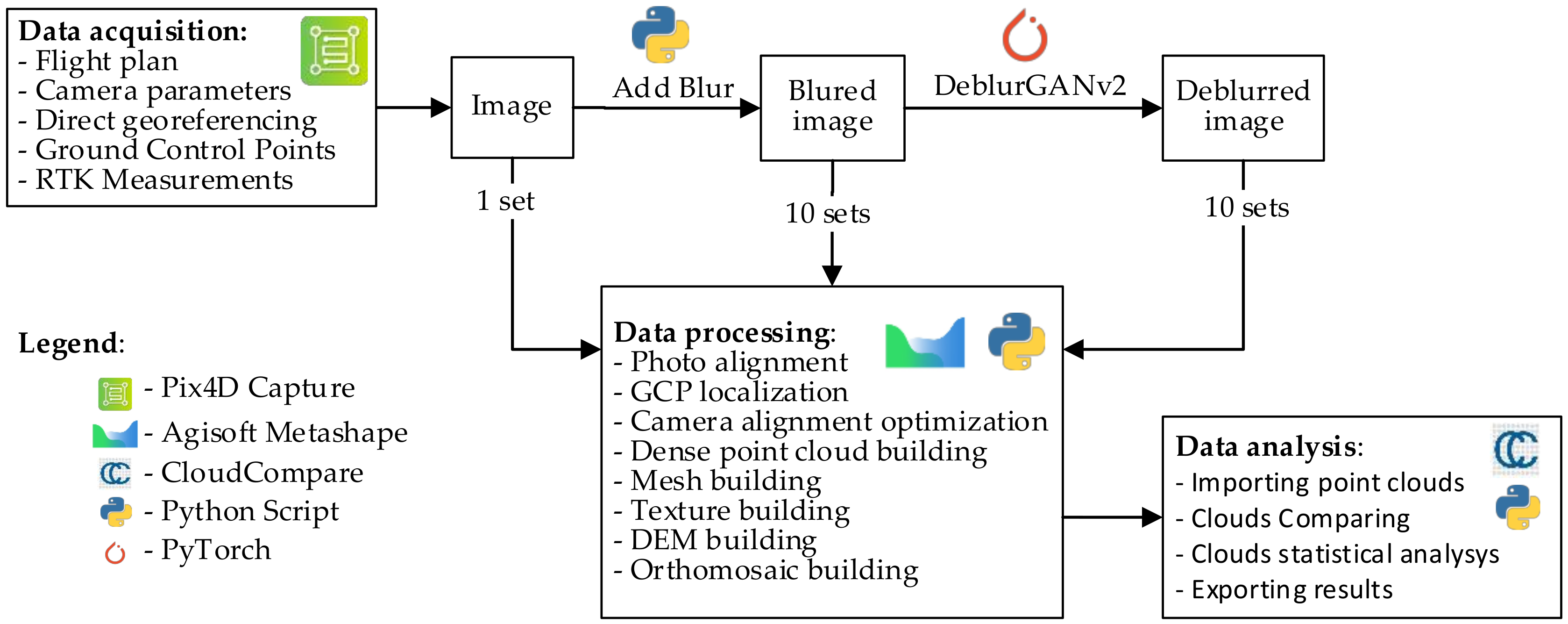
Figure 3.
Reference model: (a) orthoimage; (b) digital surface model (DSM).

Figure 4.
Ground control point No. 1—visual comparison of blur with a varying kernel and a corresponding DeblurGANv2 method image.
Figure 4.
Ground control point No. 1—visual comparison of blur with a varying kernel and a corresponding DeblurGANv2 method image.

Figure 5.
Cars parked within the measurement area—visual comparison of blur with a varying kernel and a corresponding DeblurGANv2 method image.
Figure 5.
Cars parked within the measurement area—visual comparison of blur with a varying kernel and a corresponding DeblurGANv2 method image.

Figure 6.
Image quality evaluator score changes: (a) blind referenceless image spatial quality evaluator (BRISQUE), natural image quality evaluator (NIQE) and perception-based image quality evaluator (PIQE); (b) no-reference perceptual blur metric (NRPBM).
Figure 6.
Image quality evaluator score changes: (a) blind referenceless image spatial quality evaluator (BRISQUE), natural image quality evaluator (NIQE) and perception-based image quality evaluator (PIQE); (b) no-reference perceptual blur metric (NRPBM).

Figure 7.
Comparison of reported survey data for blurred and deblurred data set: (a) the number of tie points; (b) the number of projections; (c) reprojection error (pix); (d) camera location total error (m); (e) GCP total RMSE (cm); and (f) the number of marked GCPs.
Figure 7.
Comparison of reported survey data for blurred and deblurred data set: (a) the number of tie points; (b) the number of projections; (c) reprojection error (pix); (d) camera location total error (m); (e) GCP total RMSE (cm); and (f) the number of marked GCPs.

Figure 8.
Textured model—visual comparison of the product part developed using photos with a varying blur kernel and their corresponding product, after the application of the method.
Figure 8.
Textured model—visual comparison of the product part developed using photos with a varying blur kernel and their corresponding product, after the application of the method.

Figure 9.
Solid model—visual comparison of the product part developed using photos with a varying blur kernel and their corresponding product, after the application of the method.
Figure 9.
Solid model—visual comparison of the product part developed using photos with a varying blur kernel and their corresponding product, after the application of the method.

Figure 10.
Orthoimage—visual comparison of a product part developed using photos with a varying blur kernel and their corresponding product, after the application of the method.
Figure 10.
Orthoimage—visual comparison of a product part developed using photos with a varying blur kernel and their corresponding product, after the application of the method.

Figure 11.
M3C2 distances, calculated relative to the reference cloud, scale in meters.

Figure 12.
M2C2 distances change: (a) mean values; (b) standard deviation.


Table 1.
Accuracy data of the developed reference model.
| Flight Altitude | Ground Resolution | Tie Points | Projections | Reprojection Error |
|---|---|---|---|---|
| 74.5 m | 2.45 cm/pix | 416,194 | 1,515,694 | 1.09 pix |
| Camera locations and error estimates | ||||
| X error (m) | Y error (m) | Z error (m) | XY error (m) | Total error (m) |
| 1.01606 | 2.70717 | 112.933 | 2.89156 | 112.97 |
| GCP locations and error estimates | ||||
| X error (cm) | Y error (cm) | Z error (cm) | XY error (cm) | Total (cm) |
| 1.35198 | 0.928474 | 0.14282 | 1.6401 | 1.6463 |
Table 2.
Reported survey data for blurred dataset.
| Blur Kernel | Flying Altitude (Reported) (m) | Ground Resolution (cm/pix) | Tie Points | Projections | Reprojection Error (pix) |
|---|---|---|---|---|---|
| 0 | 74.5 | 2.45 | 416,194 | 1,515,694 | 1.09 |
| 5 | 75.6 | 2.69 | 459,985 | 1,703,465 | 1.01 |
| 10 | 75.9 | 2.69 | 468,013 | 1,762,049 | 0.969 |
| 15 | 157 | 2.44 | 473,566 | 1,781,602 | 6.95 |
| 20 | 129 | 2.49 | 451,838 | 1,648,334 | 6.16 |
| 25 | 79.3 | 2.64 | 424,529 | 1,503,363 | 1.12 |
| 30 | 70.6 | 2.72 | 402,741 | 1,380,426 | 1.17 |
| 35 | 10 000 | 724 | 378,829 | 1,255,205 | 1.24 |
| 40 | 79.6 | 2.65 | 363,984 | 1,169,618 | 1.18 |
| 45 | 79.6 | 2.65 | 346,471 | 1,089,462 | 1.19 |
| 50 | 81.1 | 2.7 | 335,285 | 1,030,242 | 2.99 |
Table 3.
Average camera location error. X—Easting. Y—Northing. Z—Altitude.
| Blur Kernel | X Error (m) | Y Error (m) | Z Error (m) | XY Error (m) | Total Error (m) |
|---|---|---|---|---|---|
| 0 | 1.01606 | 2.70717 | 112.933 | 2.89156 | 112.97 |
| 5 | 1.05511 | 2.6617 | 113.921 | 2.8632 | 113.957 |
| 10 | 1.04322 | 2.65756 | 114.203 | 2.85498 | 114.238 |
| 15 | 25.839 | 31.9469 | 204.859 | 41.0884 | 208.939 |
| 20 | 19.5152 | 25.4927 | 175.837 | 32.1048 | 178.744 |
| 25 | 1.30977 | 2.6244 | 118.957 | 2.93308 | 118.993 |
| 30 | 0.945613 | 2.91196 | 108.394 | 3.06164 | 108.437 |
| 35 | 0.988093 | 3.01637 | 106.259 | 3.17409 | 106.306 |
| 40 | 1.14262 | 2.60115 | 118.828 | 2.84105 | 118.862 |
| 45 | 1.03106 | 3.17542 | 118.685 | 3.33862 | 118.732 |
| 50 | 10.9788 | 7.90267 | 120.892 | 13.5273 | 121.646 |
Table 4.
Control points root mean square error (RMSE). X—Easting. Y—Northing. Z—Altitude.
| Blur Kernel | GCP Count | X Error (cm) | Y Error (cm) | Z Error (cm) | XY Error (cm) | Total (cm) |
|---|---|---|---|---|---|---|
| 0 | 6 | 1.35198 | 0.928474 | 0.14282 | 1.6401 | 1.6463 |
| 5 | 6 | 1.62547 | 1.17136 | 0.17614 | 2.00356 | 2.01128 |
| 10 | 6 | 1.82308 | 1.1612 | 0.213706 | 2.16148 | 2.17202 |
| 15 | 6 | 27.0598 | 35.9852 | 11.3785 | 45.0241 | 46.4396 |
| 20 | 6 | 22.1977 | 33.1699 | 13.7652 | 39.9122 | 42.2192 |
| 25 | 4 | 1.57333 | 0.498542 | 0.188985 | 1.65043 | 1.66121 |
| 30 | 5 | 0.961179 | 0.830387 | 0.414181 | 1.2702 | 1.33602 |
| 35 | 4 | 0.797182 | 0.634285 | 0.278878 | 1.01873 | 1.05621 |
| 40 | 3 | 1.45667 | 0.158248 | 0.237339 | 1.46525 | 1.48434 |
| 45 | 3 | 1.19554 | 0.308544 | 0.237474 | 1.23471 | 1.25734 |
| 50 | 3 | 2.70446 | 3.85804 | 0.234899 | 4.71154 | 4.71739 |
Table 5.
Calculated image quality evaluator scores.
| Kernel | Blur | Deblur | ||||||
|---|---|---|---|---|---|---|---|---|
| BRISQUE | NIQE | PIQE | NRPBM | BRISQUE | NIQE | PIQE | NRPBM | |
| 0 | 32.5371 | 3.3942 | 20.1403 | 0.2464 | 32.5371 | 3.3942 | 20.1403 | 0.2464 |
| 5 | 40.1396 | 5.3276 | 35.7262 | 0.4279 | 39.0127 | 4.8747 | 24.6537 | 0.3461 |
| 10 | 41.0298 | 5.9315 | 62.2739 | 0.5734 | 42.9720 | 4.9778 | 24.1605 | 0.3548 |
| 15 | 41.9970 | 5.8995 | 71.8718 | 0.5927 | 43.1827 | 5.1326 | 28.7600 | 0.3461 |
| 20 | 42.3787 | 5.9203 | 76.7909 | 0.5951 | 43.1036 | 5.1680 | 29.8516 | 0.3527 |
| 25 | 42.6260 | 5.9928 | 79.3120 | 0.5933 | 43.7847 | 5.1275 | 30.7244 | 0.3613 |
| 30 | 42.8275 | 5.8444 | 80.7251 | 0.5880 | 45.2656 | 4.9797 | 31.9076 | 0.3775 |
| 35 | 42.8824 | 5.9419 | 81.4176 | 0.5820 | 45.8312 | 4.8937 | 34.4529 | 0.3956 |
| 40 | 43.0532 | 5.9418 | 82.2514 | 0.5741 | 46.0060 | 4.9044 | 35.9615 | 0.3899 |
| 45 | 43.1581 | 5.9602 | 82.6866 | 0.5662 | 46.4773 | 4.9784 | 35.7911 | 0.3712 |
| 50 | 43.1872 | 5.9524 | 83.2577 | 0.5573 | 46.7075 | 5.0238 | 36.4373 | 0.3521 |
Table 6.
Reported survey data for a deblurred dataset.
| Deblur | Flying Altitude (Reported) (m) | Ground Resolution (cm/pix) | Tie Points | Projections | Reprojection Error (pix) |
|---|---|---|---|---|---|
| 0 | 74.5 | 2.45 | 416,194 | 1,515,694 | 1.09 |
| 5 | 75.1 | 2.69 | 442,180 | 1,645,007 | 1.04 |
| 10 | 75.3 | 2.69 | 457,941 | 1,665,776 | 1.01 |
| 15 | 74.7 | 2.7 | 453,347 | 1,624,915 | 1.07 |
| 20 | 72.8 | 2.7 | 437,927 | 1,497,823 | 1.16 |
| 25 | 79.8 | 2.66 | 433,953 | 1,422,424 | 1.19 |
| 30 | 79.8 | 2.65 | 425,342 | 1,328,750 | 1.25 |
| 35 | 79.7 | 2.65 | 411,533 | 1,220,397 | 1.29 |
| 40 | 79.7 | 2.65 | 387,720 | 1,109,842 | 1.32 |
| 45 | 79.6 | 2.65 | 344,131 | 970,994 | 1.4 |
| 50 | 79.1 | 2.63 | 300,779 | 834,237 | 1.57 |
Table 7.
Average camera location error (X—Easting, Y—Northing, Z—Altitude).
| Deblur | X Error (m) | Y Error (m) | Z Error (m) | XY Error (m) | Total Error (m) |
|---|---|---|---|---|---|
| 0 | 1.01606 | 2.70717 | 112.933 | 2.89156 | 112.97 |
| 5 | 1.04393 | 2.67472 | 113.69 | 2.87122 | 113.726 |
| 10 | 1.04606 | 2.67152 | 113.843 | 2.86902 | 113.879 |
| 15 | 1.02665 | 2.7201 | 112.912 | 2.9074 | 112.95 |
| 20 | 0.952102 | 2.79801 | 111.177 | 2.95557 | 111.216 |
| 25 | 1.21931 | 2.51578 | 118.919 | 2.79569 | 118.952 |
| 30 | 1.22138 | 2.49247 | 118.929 | 2.77563 | 118.961 |
| 35 | 1.21005 | 2.47763 | 118.963 | 2.75733 | 118.995 |
| 40 | 1.1795 | 2.56589 | 118.892 | 2.824 | 118.925 |
| 45 | 1.16576 | 2.58083 | 118.88 | 2.83191 | 118.914 |
| 50 | 1.12633 | 2.56772 | 118.647 | 2.80389 | 118.68 |
Table 8.
Control points RMSE (X—Easting, Y—Northing, Z—Altitude).
| Deblur | Count | X Error (cm) | Y Error (cm) | Z Error (cm) | XY Error (cm) | Total (cm) |
|---|---|---|---|---|---|---|
| 0 | 6 | 1.35198 | 0.928474 | 0.14282 | 1.6401 | 1.6463 |
| 5 | 6 | 1.52361 | 1.04413 | 0.16942 | 1.84705 | 1.85481 |
| 10 | 6 | 1.67629 | 1.13808 | 0.200033 | 2.02612 | 2.03597 |
| 15 | 6 | 1.53698 | 1.06043 | 0.183753 | 1.8673 | 1.87632 |
| 20 | 6 | 1.12107 | 0.638714 | 0.159253 | 1.29025 | 1.30004 |
| 25 | 6 | 1.13649 | 0.865287 | 0.184179 | 1.4284 | 1.44023 |
| 30 | 6 | 0.959562 | 0.893345 | 0.152415 | 1.31104 | 1.31987 |
| 35 | 6 | 0.75247 | 0.752481 | 0.133251 | 1.06416 | 1.07247 |
| 40 | 5 | 6.13895 | 6.27537 | 1.35764 | 8.77878 | 8.88314 |
| 45 | 5 | 4.35626 | 4.75946 | 1.36225 | 6.45209 | 6.59433 |
| 50 | 5 | 3.36417 | 3.03876 | 1.38842 | 4.5334 | 4.74125 |
Table 9.
Calculated M3C2 distances.
| Kernel | Blur | Deblur | ||
|---|---|---|---|---|
| Mean | Std. Deviation | Mean | Std. Deviation | |
| 5 | −0.047 | 0.7171 | −0.0415 | 0.6335 |
| 10 | −0.0732 | 0.8571 | −0.0495 | 0.6745 |
| 15 | −3.2327 | 13.6939 | −0.0074 | 0.8452 |
| 20 | 1.0668 | 12.6647 | 0.0464 | 0.8117 |
| 25 | −0.288 | 1.0104 | −0.2643 | 0.8803 |
| 30 | 0.1825 | 1.0667 | −0.285 | 0.9579 |
| 35 | 0.3792 | 1.1389 | −0.3187 | 1.0308 |
| 40 | −0.1491 | 1.0717 | −0.2452 | 1.0806 |
| 45 | 0.1205 | 2.2933 | −0.2366 | 1.1688 |
| 50 | −3.7489 | 14.1588 | −0.2758 | 1.1695 |
© 2020 by the author. Licensee MDPI, Basel, Switzerland. This article is an open access article distributed under the terms and conditions of the Creative Commons Attribution (CC BY) license (http://creativecommons.org/licenses/by/4.0/).
Share and Cite
MDPI and ACS Style
Burdziakowski, P. A Novel Method for the Deblurring of Photogrammetric Images Using Conditional Generative Adversarial Networks. Remote Sens. 2020, 12, 2586. https://0-doi-org.brum.beds.ac.uk/10.3390/rs12162586
AMA Style
Burdziakowski P. A Novel Method for the Deblurring of Photogrammetric Images Using Conditional Generative Adversarial Networks. Remote Sensing. 2020; 12(16):2586. https://0-doi-org.brum.beds.ac.uk/10.3390/rs12162586
Chicago/Turabian StyleBurdziakowski, Pawel. 2020. "A Novel Method for the Deblurring of Photogrammetric Images Using Conditional Generative Adversarial Networks" Remote Sensing 12, no. 16: 2586. https://0-doi-org.brum.beds.ac.uk/10.3390/rs12162586
Note that from the first issue of 2016, this journal uses article numbers instead of page numbers. See further details here.