Variations of Mass Balance of the Greenland Ice Sheet from 2002 to 2019
by
 , and
, and
Yaqiong Mu
1,2, 
Yanqiang Wei
3,
Jinkui Wu
1,2,*,
Yongjian Ding
1,2,
Donghui Shangguan
2,4 and
Di Zeng
1,2 1
Key Laboratory of Eco-Hydrology of Inland River Basin, Northwest Institute of Eco-Environment and Resources, Chinese Academy of Sciences, Lanzhou 730000, China
2
College of Resources and Environment, University of Chinese Academy of Sciences, Beijing 100049, China
3
Key Laboratory of Remote Sensing of Gansu Province, Northwest Institute of Eco-Environment and Resources, Chinese Academy of Sciences, Lanzhou 730000, China
4
Cold and Arid Regions Environmental and Engineering Research Institute, Chinese Academy of Sciences, Lanzhou 730000, China
*
Author to whom correspondence should be addressed.
Remote Sens. 2020, 12(16), 2609; https://0-doi-org.brum.beds.ac.uk/10.3390/rs12162609
Submission received: 24 July 2020
/
Accepted: 10 August 2020
/
Published: 13 August 2020
(This article belongs to the Section Environmental Remote Sensing)
Abstract
:The melting of the polar ice caps is considered to be an essential factor for global sea-level rise and has received significant attention. Quantitative research on ice cap mass changes is critical in global climate change. In this study, GRACE JPL RL06 data under the Mascon scheme based on the dynamic method were used. Greenland, which is highly sensitive to climate change, was selected as the study area. Greenland was divided into six sub-research regions, according to its watersheds. The spatial–temporal mass changes were compared to corresponding temperature and precipitation statistics to analyze the relationship between changes in ice sheet mass and climate change. The results show that: (i) From February 2002 to September 2019, the rate of change in the Greenland Ice Sheet mass was about −263 ± 13 Gt yr−1 and the areas with the most substantial ice sheet loss and climate changes were concentrated in the western and southern parts of Greenland. (ii) The mass balance of the Greenland Ice Sheet during the study period was at a loss, and this was closely related to increasing trends in temperature and precipitation. (iii) In the coastal areas of western and southern Greenland, the rate of mass change has accelerated significantly, mainly because of climate change.
1. Introduction
The two poles of the Earth are vast ice freshwater storehouses. Ice sheets account for about 97% of the area of global glaciers and 99% of the total ice volume. At the same time, like other glaciers, ice sheets in the polar regions also record and provide early warnings of climate change. Because of the continued warming of the global climate and other reasons, Greenland and Antarctica currently contribute to the global average sea-level rise [1]. The Special Report on the Ocean and Cryosphere in a Changing Climate (SROCC) released by the Intergovernmental Panel on Climate Change (IPCC) in 2019 pointed out that the mass of polar and mountain glaciers and ice caps was in continuous decline and that ocean heating was intensifying. Melting continues to expand, thereby accelerating the rate of sea-level rise. From 1902 to 2015, global sea level rose by 16 cm, of which the 3.6 cm that occurred between 2006 and 2015 is about 2.5 times higher than the average growth rate from 1901 to 1990. The rate of sea-level rise caused by the loss of glaciers and ice sheets from 2006 to 2015 was about 1.8 mm yr−1, becoming the leading cause of the sea-level rise. Compared to the period from 1997 to 2006, the loss of Antarctic ice sheet ice from 2007 to 2016 has tripled. The mass balance of the Greenland Ice Sheet has decreased more than twice since the 21st century compared to the 20th century [2,3]. Greenland is the largest island in the world. The Greenland Ice Sheet covers 81% of Greenland, taking up an area of about 1.8 × 10⁶ km2, with an average thickness of about 1.5 × 10³ m. The Greenland Ice Sheet is the second-largest ice sheet in the world after the Antarctic Ice Sheet [4]. At present, the Greenland Ice Sheet has a severe mass loss linked to increases in annual temperature, precipitation anomalies, combined with surface water runoff and iceberg collapse. This change in mass balance is much more significant than what would be possible with changes caused by precipitation alone [5]. As the mass of the ice sheet changes, vast amounts of methane contained in the Arctic permafrost are released, promoting greenhouse gas effects and further aggravating global warming of the earth [6]. Studies have shown that if the Greenland ice sheet were to melt completely in the 21st century, it would cause a global sea-level rise of about 6.5~7.4 m [7,8]. Therefore, understanding the changes in the mass balance of the bipolar ice sheets and their relationship with climate change is critical for our understanding of global climate change and to refine sea-level predictions [9].
The study of changes in ice sheet mass balance requires effective and precise observation methods. Tools for measuring mass balance such as Global Navigation Satellite System (GNSS) and Interferometric Synthetic Aperture Radar (InSAR) are only suitable for small-scale deployment. With the development of satellite altimetry [10], three main methods become available for determining the mass balance change of ice sheets: elevation measurement, direct measurement, and the mass balance method. The elevation measurement method uses laser altimetry satellites such as ICESat and microwave altimetry satellites such as ERS-1 to measure ice cap elevation changes and then measure ice sheet mass balance changes. Height measurement technology is constantly improving. ICESat-2, released in 2015, can be used to quantify the amount of change in ice sheets and sea ice. At present, elevation measurements still need to use more refined correction models and data processing methods to improve data mass; the direct measurement method relies on the GRACE gravity satellites to directly obtain time-varying gravity field information of the study area, which can accurately measure the spatial and temporal changes of surface fluids, underground runoff and solid water mass [11,12,13]. The GRACE satellite not only provides high-precision medium- and long-wavelength earth gravity fields, but can also give the time-variation of medium- and long-wave gravity fields, and can be used as a relatively direct method for the quantitative analysis of ice cap mass changes [14]. GRACE’s early studies inferred changes in land water reserves through changes in gravity field mass. Wahr et al. (1998) first expressed the change in surface mass as the equivalent water height and established the relationship between the time-varying gravity field coefficient and the change in surface mass density [15]. Since then, many researchers have applied the GRACE gravity satellite method to quantitatively study changes in the polar ice sheets. Using GRACE’s global time-varying gravitational field information, it is possible to detect the mass migration of the worldwide system and study the changes in the mass balance of the Greenland Ice Sheet [16]. For example, Ramillien et al. (2006) used gravity satellite data to find that Greenland’s contribution to sea-level rise from July 2002 to March 2005 was 0.36 ± 0.04 mm yr−1 [17]. Velicogna et al. (2006) used gravity satellite data from April 2002 to April 2006 to independently estimate the contribution of Greenland’s ice loss to sea-level changes. They detected an ice loss of 248 ± 36 km3 yr−1, which is equivalent to a global sea-level rise of 0.5 ± 0.1 mm yr−1 [18]. The study by Tapley et al. (2019) showed that from April 2002 to June 2017, the average annual ice loss in Greenland was −258 ± 26 Gt yr−1, and the interannual variation was −137 Gt yr−1 [19]. It should be pointed out that there are apparent differences in the Greenland Ice Sheet melting rates given by different scholars based on GRACE time-varying gravity. The contribution is in the range of 0.36~0.50 mm yr−1 [18,20,21] Even within the different periods, using the same type of GRACE data still leads to errors in the results. Generally, the source of error is not only the difference in the research period, as for the same data product, the error obtained during the same period is relatively large. The errors are mostly caused by the use of different inversion methods, such as the traditional spherical harmonic method. This study uses the data under the Mascon scheme, which can effectively avoid errors caused by traditional data processing.
This study was based on GRACE Level-2 RL06 (Coastal Resolution Improvement CRI) data provided by the Jet Propulsion Laboratory (JPL) using the Mascon scheme to determine the changes in the mass balance of the Greenland Ice Sheet during the period from April 2002 to September 2019. Based on the data of six sub-regions, the spatial and temporal distribution characteristics of the overall and local mass changes of the Greenland Ice Sheet were analyzed. Using the long-range reanalysis of meteorological data from the Centre for Environmental Data Analysis (CEDA), the climate data of the Greenland Ice Sheet during the 1990s (1990–2000) and 2010s (2011–2018) were analyzed to discuss the relationship between the melting of the ice and climate change, and the extent to which the ice sheet in Greenland responds to climate change. To analyze and predict future sea-level changes, it is important to understand the characteristics of the ice cover, and the sensitivity of the changes in the mass balance of the ice cover to temperature as well as precipitation.
2. Materials and Methods
2.1. Research Area
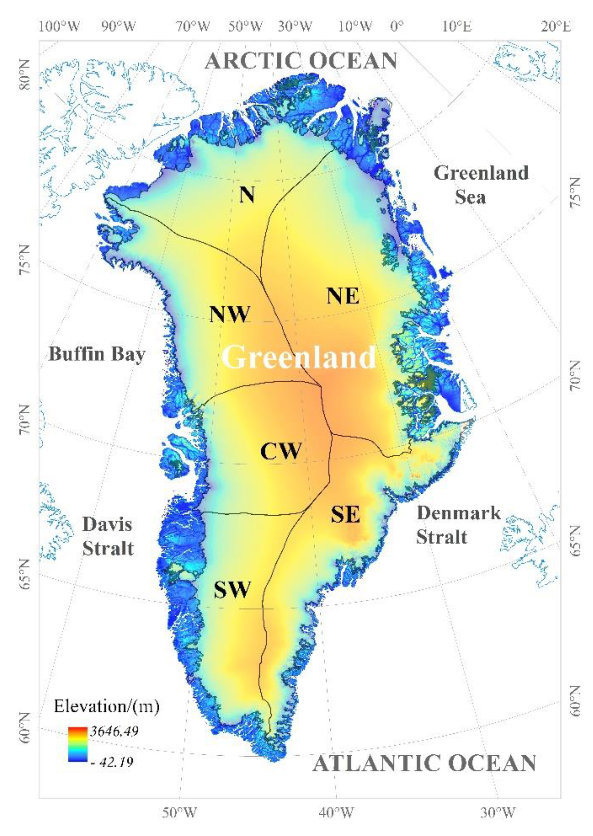
Greenland, located northeast of North America, lies between the Arctic Ocean and the Atlantic Ocean (Figure 1), within 59°44′42′′–83°39′46′′N and 73°15′13′′–11°20′11′′W. The total length of its coastline is 49,200 km and the highest elevation of the inland area is about 3300 m [22]. The total study area is approximately 1.786 × 10⁶ km2. About three-quarters of the island lies north of the Arctic Circle and has a typical cold climate year-round. The annual average temperature is below 0 °C, and the average winter temperature (January) is −6 °C in the south and −35 °C in the north. The average summer temperature in the southwestern coast is 8 °C, while it is 3.6 °C at the highest point of the ice sheet. The average annual precipitation decreases from 1900 mm in the south to about 50 mm in the north. The continental glaciers (or ice sheets) of Greenland have an area of 1.813 × 10⁶ km2, and the average thickness of the ice layer reaches 2300 m, which is similar to the average thickness of the Antarctic continental ice sheet. The total volume of ice and snow contained over Greenland is 3.0 × 10⁶ km3, accounting for 5.4% of the total global freshwater. The ice-free area of Greenland is 441,700 km2, but most of it is represented by wastelands in the north and east coasts [23].
Ice sheet loss is the most significant environmental problem of Greenland. Research has shown that Greenland has lost 3800 Gt of ice since 1992, enough to increase global sea level by 10.6 mm. The rate of ice loss increased from 33 Gt per year in the 1990s to 254 Gt per year in the last decade, growing sevenfold in three decades [24].
For this study, we used the regional boundaries from the Greenland drainage basin and ice sheet definitions produced by E. Rignot and J. Mouginot and used by IMBIE 2016 [25,26]. Elevation data were from a composite product of Cryosat-2 elevation measurements and the 5-m resolution digital elevation model (DEM) provided by the Polar Geospatial Center [27].
2.2. Introduction to the Data
The GRACE gravity satellites can detect changes in global land water reserves according to a specific resolution. There are multiple GRACE data sets. The GRACE RL06 Coastal Resolution Improvement (CRI) series data used in this study were published by JPL from April 2002 to September 2019 [28]. The horizontal resolution of the data is 1°, and there are 177 months of useful data. The data are given in equivalent water thickness (unit: cm) [29,30,31]. In this manuscript, JPL RL06 (CRI) data uses the Mascon solution based on the principle of dynamics, which provides a monthly gravity field change generated by 4551 equal-area 3° grids, of the size of about 330 km; a coastline resolution is applied to improve filtering (CRI) to separate the mass of land and ocean from a single mascon across the coastline. A solution based on Level 1B data replaces the C20 measured by GRACE satellites with C20 items from SLR data [32] and the Peltier ICE6G-D model [33]. In this approach the data plan has completed the glacier isostatic pressure adjustment (GIA) correction, improving the results from the inversion mass change. The final JPL RL06 data is in the NetCDF format with a spatial resolution of 1° [34,35].
Long-record meteorological station data were selected from the long-sequence reanalysis data of the Environmental Data Analysis Center (CEDA) [36], and the Coupled Model Inter-comparison Project version 6 (CMIP6) was used to represent the future climate [37,38]. The Climatic Research Unit (CRU) dataset was provided by the University of East Anglia. The data set included daily average temperature, precipitation, and other regular meteorological variables. The data, with a spatial resolution of 0.5° × 0.5°, included two periods, one from 1991 to 2000 and one from 2010 to 2018. The model data were obtained from the CCSM4 (Community Climate System Model, CCSM) model in the Coupled Model Inter-comparison Project version 5 (CMIP5). We used the Representative Concentration Pathway version 4.5 (RCP4.5) scenario: 2050 and 2070 temperature and precipitation predictions correspond to climate change scenario results from 2041 to 2050 and 2061 to 2070, respectively. The average monthly temperature and precipitation values in the two periods were used to evaluate the model space simulation performance. Climate variables included monthly temperature and total monthly precipitation.
2.3. Mascon Method
There are two mainstream schemes for performing GRACE data inversion of the polar ice sheet to quantify mass balance changes. One is the method based on the spherical harmonic coefficient of the earth’s gravity field, in which the surface mass change is retrieved by the spherical harmonic factor of the gravity field [39]. The other scheme is based on the Mascon method for obtaining local or global mass changes based on GRACE Level 1B data. This scheme is proposed based on inter-satellite observation data [40,41]. The data expression forms of the two main inversion methods include equivalent water height, gravity anomaly, changes in the earth’s leveling surface, and surface deformation. The name Mascon method comes from the abbreviations of mass and concentration. Its essence is to divide the research area into several blocks according to a certain regular shape. The mass in any block is evenly distributed. The block mass change is the Mascon parameter. The set Mascon parameter can reflect the global surface mass change. The Mascon method is mainly used to recover abnormal surface mass, adjust the gravity solution, and effectively suppress related errors. Using spherical crown mass concentration elements (mascons) to resolve mass changes relies on external information provided by near-global geophysical models to constrain the solution. Owing to more effective signals retained, which are smoother than those from the spherical harmonic coefficient method, the spatial resolution is higher [30].
After reading and processing the GRACE JPL RL06 data, the GRCTellus JPL-Mascons is used to complete the glacier isostatic adjustment. To improve the coastline error, the Coastal Resolution Improvement (CRI) coastline resolution improvement can be used to separate the land and ocean mass in Oceania across the coastline. For Greenland and Antarctica, the mass flux along the coastline is greater than the adjacent ocean dynamics signal. Therefore, CRI filters are used in these areas and the remaining mass is placed in the mascon on the ice sheet, effectively reducing by about 80% the large loss errors due to the mass loss trend of export glaciers [31].
The GRACE inter-satellite distance variability observation data is used to invert the earth’s time-varying gravity field based on the Mascon method. This approach has been used to invert regional surface mass changes, including Antarctic ice sheet mass changes and Greenland glacier melting, [42,43]. The Greenland Ice Sheet contains 25 small areas. Based on this integration, Greenland is divided into six patches or “mass blocks” (Figure 1), and the surface density changes within each patch over time. The change in mass per unit area is assumed to be spatially uniform. Therefore, the total mass anomaly in each patch can be represented by the product of the surface density anomaly and the patch area, and the mass anomaly is calculated independently each month.
2.4. Data Experiments
In this manuscript, to obtain the mass change of the Greenland ice sheet, we used the GRCTellus JPL-Mascons (CRI) processing program provided by the GRACE TELLUS website. In this part, we explain the entire process of GRACE data processing. Most of the data processed by GRACE is based on the basic theory of GRACE time-varying gravity satellites. The basic theory was proposed by Wahr et al. on the inversion of surface mass changes by Grace time-varying gravity satellites [44]. Due to the stagnation of solid earth characteristics, the change of its surface load will cause a change of the geosphere, which will affect the change of the geoid, and establish the relationship between the density of the geoid and the unit area. The geoid represents the earth’s gravity field. Based on the time-varying gravity field, the basic equation for retrieving the change of the surface mass of the earth is:
According to Wahr’s theory [44], the GRACE time-varying gravity field model can inversely obtain the change in areal density at any point on the thin layer of earth’s surface mass:
where θ and φ are the geocentric latitude and longitude, respectively, a is the average radius of the earth, is the average density of the earth, l and m are the order and power, and is the standardized associated Legendre function, kl is Love’s load number, and ΔClm and ΔSlm are the changes of the dimensionless normalized spherical harmonic coefficient with respect to the mean value of the time-varying gravity field, respectively.
The mass change of the earth’s surface obtained by the two equations is converted into the mass change expressed in equivalent water height, and the formula for the equivalent water thickness of the data variable is:
where EWT is the equivalent water height, Δσ(θ,φ) is the amount of change in the mass of the earth’s surface, and is the mass element density.
After obtaining the necessary mass change data, we calculate the anomalies in surface mass in the selected area. The time series were analyzed with the least square method to fit the slope of the annual average mass change of the entire domain and regions. To clearly understand the spatial change trend of the Greenland Ice Sheet, the grid-by-grid trend analysis can intuitively reflect its spatial change trend, and can better reflect the difference in time series of each grid. It is an effective way to study the change in the mass balance of the Greenland Ice Sheet.
3. Results
3.1. Spatial Trend of the Overall Mass of the Greenland Ice Sheet
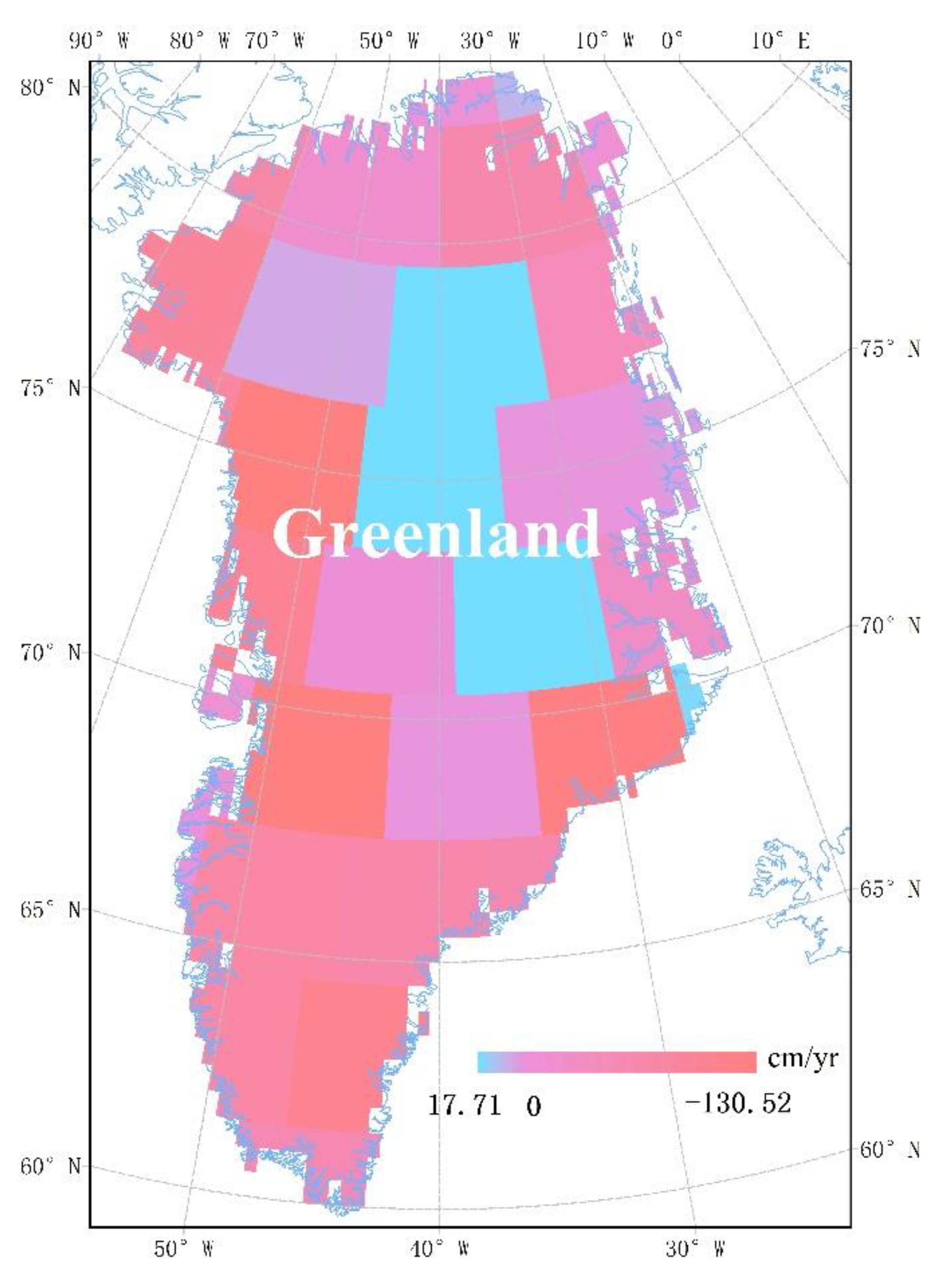
Using GRACE time-varying gravity field data through the Mascon inversion model, we analyzed the spatial trends in ice sheet mass after deducting the influence of GIA from April 2002 to September 2019 (Figure 2). Overall, the Greenland Ice Sheet shows a clear melting trend. The area with the largest annual average melting shows a loss as high as 1.305 × 103 mm yr−1. At the same time, there are obvious regional differences. The areas with relatively significant mass losses are mainly concentrated in the west and south, followed by ablation in the east, while ablation in the central area is relatively weak; there are also some areas where the mass has increased slightly. In general, the melting trend of the Greenland Ice Sheet shows that it is more pronounced at the edges than in the middle, greater in the south than in the north, and in the west than in the east (Figure 2).
The temporal mass change trend of the Greenland Ice Sheet from February 2002 to September 2019 was quantified by linearly fitting the Greenland Ice Sheet mass change sequence. It can be seen from Figure 3 that since 2002, the overall mass loss of the Greenland Ice Sheet has shown a trend of several-fold increase. Taking 2007 as the node, the mass change of the Greenland Ice Sheet has increased about 1000 Gt, and then gradually decreased by nearly 4000 Gt.
The Greenland Ice Sheet mass change rate is computed at annual intervals from time series of relative mass change using a 3-yr window. The average annual melting rate of the ice sheet reached −263.42 ± 22 Gt yr−1, with an acceleration of −41.45 ± 1.89 Gt yr−1. After it almost doubled to the highest value in 2012, the rate gradually slowed down after 2013 due to changes in atmospheric conditions. Judging from the overall trend, the ablation of the Greenland Ice Sheet is intensifying.
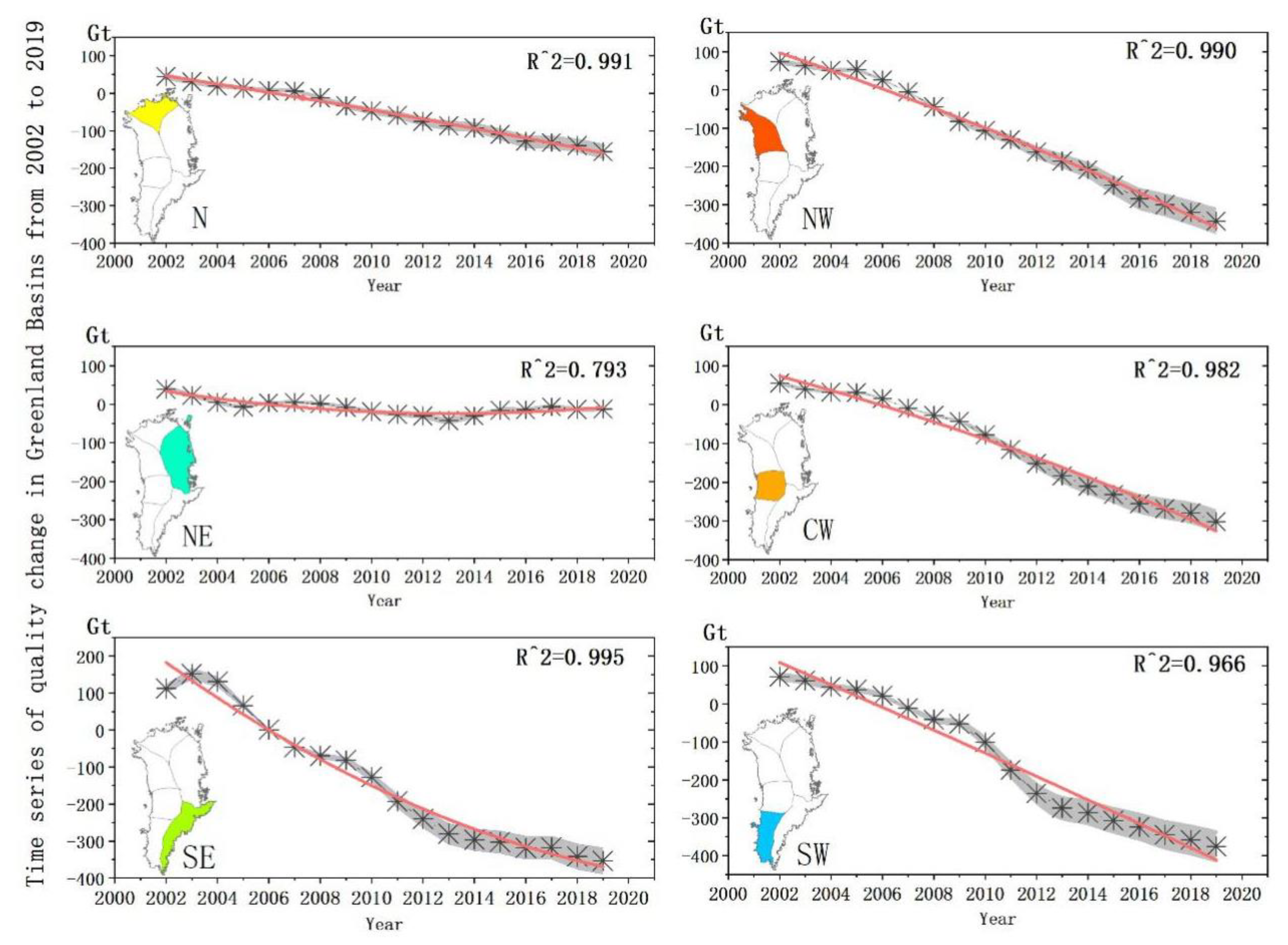
3.2. Change in Inter-Annual Mass by Region
To further analyze the uneven temporal and spatial ice sheet mass changes in Greenland, we adopted the watershed and ice sheet zoning produced by Rignot and Mouginot and used by NASA IMBIE 2016 [27]. The zoning scheme divides Greenland into six different watersheds. Figure 4 shows the mass change of the six watersheds of the Greenland Ice Sheet, indicating marked regional differences. Since the areas with significant mass changes are concentrated in the southern and coastal regions, it is speculated that global warming had a more significant effect on the mass ablation of Greenland’s northern and high-altitude regions, and the increase in temperature may have been the dominant factor in mass ablation.
To further analyze the spatial variation of the mass change of the Greenland Ice Sheet, it is necessary to quantify the mass ablation of each type of area. From the statistical results, it can be seen that the regions with the fastest rate of mass change are the southeast (SE) and the southwest (SW) region. The two regions each account for about 15% of the total research area. The interannual rate of change of the equivalent water height in the region from 2002 to 2019 is −0.76 × 103 mm yr−1, −0.537 × 103 mm yr−1, and the interannual mass changes were −73.591 Gt yr−1 and −69.631 Gt yr−1. These changes may be that due to the warming and melting of the ocean, and caused the retreat of the glaciers in the two regions [1]. SW is in a special sub-cold climate zone, which not only has a higher temperature than the other regions, but also presents a significant interaction between the ice sheet and the ocean, with inland ice and snow injected into the ocean through high-velocity glaciers. Although the temperature of SE is low, the elevation of the area is generally high and includes many glaciers with fast velocities. Here the response of mass changes to climate warming is more significant. The next largest mass change rate took place in NW and CW, where the inter-annual mass changes were 59.796 Gt yr−1 and −54.987 Gt yr−1. The two regions have relatively low altitude and occupy large inland areas, so the rate of mass change of the two was average. The areas with relatively small mass changes were N and NE. However, while NE accounts for up to 28.5% of the total study area, the rate of mass change was only −26.87 Gt yr−1. Figure 4 shows that NE, which includes most of the central area, was the only zone that had a mass accumulation. The mass changes were dynamic during the study period. Some of the deep central areas may have accumulated ice sheet mass [45]. Although the rate of change of mass in zone N was low, its area accounted for only half of that of zone NE. In comparison, zone N seems to have been more sensitive to climate change due to its high latitudes, and its rate of change was constant and slightly faster than that of the N zone. The time series analysis of Greenland as a whole does not reflect the regional difference in mass changes. However, after considering the analysis of different watersheds divided by factors such as the number of glaciers, the different processes of change are reflected. The spatial difference analysis from the perspective of zoning reflects the close relationship between Greenland and its geographical location and climate change in the past 20 years. On the one hand, it can be seen that the grid-based zoning analysis method can provide a more in-depth and clear analysis, allowing us to find spatial differences in mass changes. On the other hand, it can be seen that the changes in mass ablation are related to altitude, latitude, geographic location, and climate zone.
3.3. Ice Sheet Changes and Climate Change
The mass of ice sheets is affected by climate conditions and human interference. In polar regions where the ecological environment is relatively fragile, human interference is small and easily affected by climate and human factors. With global warming, there has been a marked warming phenomenon in the Arctic in the past few decades. Studies have shown that the rate of warming since the 20th century has been two to three times the global average [46]. Studies have shown that the Arctic atmospheric circulation, marine environment, and sea ice coverage have all undergone significant changes, these changes have a particular effect on the melting of the Greenland Ice Sheet surface. The warming and the continuous anomaly of the surface temperature of the Greenland Ice Sheet are directly related to the melting of its surface [47].
It can be seen that even though the Greenland Ice Sheet has been in a state of continuous mass loss, the degree varies over time, likely because of cooler atmospheric conditions and increased precipitation induced by a changing climate. We performed a simple comparison of the average results of the 2050s and 2070s simulations of the future temperature and precipitation changes in Greenland.
Unlike the rest of the Arctic, in most parts of Greenland, the annual average temperature is below 0 °C. The west and east coasts, although both located in the northern cold zone, have different climates. Most of the east and north shores (regions N/SE/SW) are almost inaccessible extreme ice sheets; the climate in the west bank is relatively milder than that in the east bank at the same latitude [48]. The average temperature is 7 °C in July and −8 °C in January.
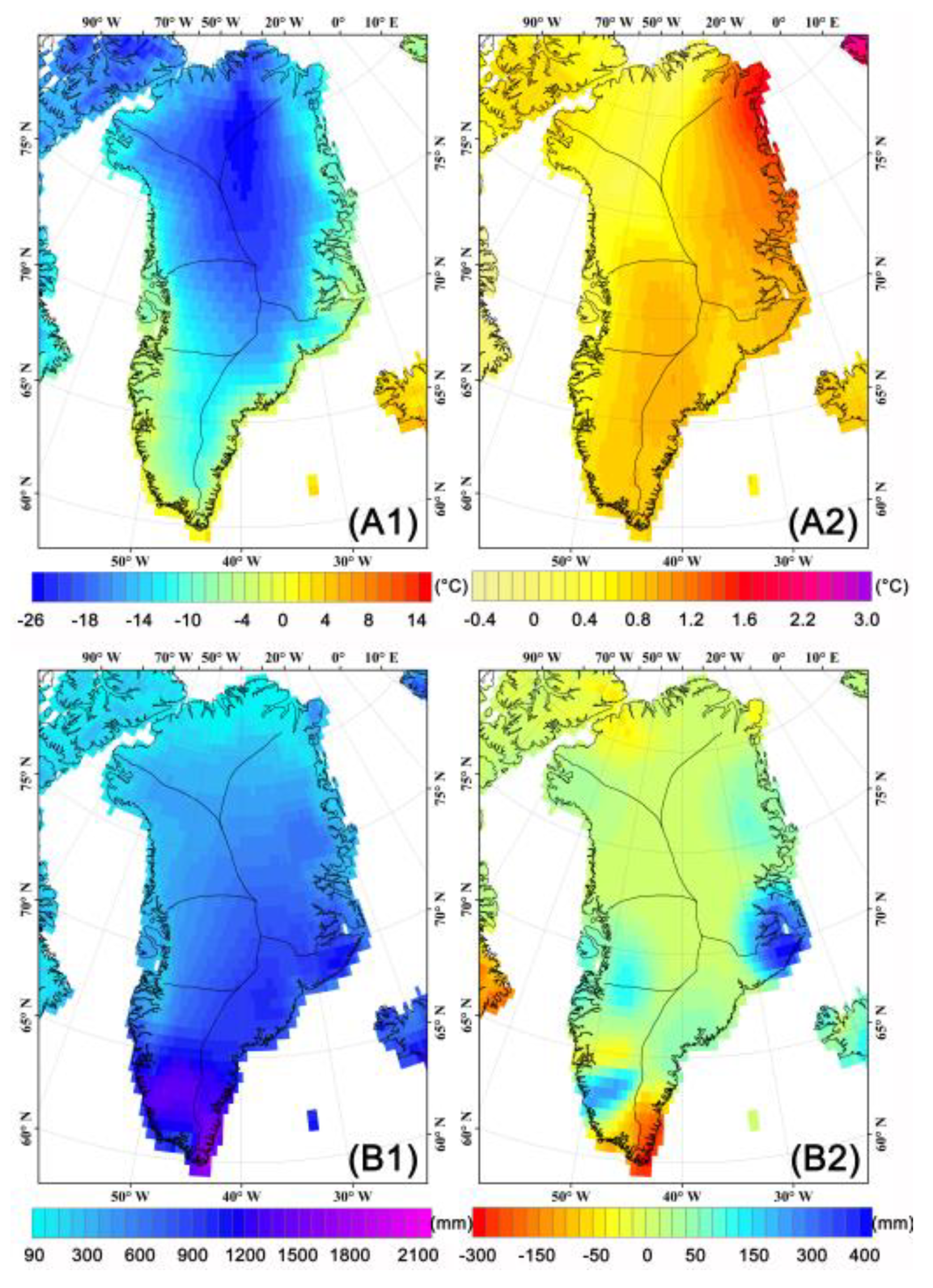
We averaged and compared the temperature and precipitation in the two research periods of 1991–2000 and 2011–2018. The final data is presented as the difference between the annual average of temperature and precipitation in the two periods (1990–2000 and 2011–2018). On this basis, the increase/decrease in temperature precipitation was calculated (Figure 5). From the overall trend, Greenland has experienced a relatively rapid warming process. The local warming of Greenland in the 21st century exceeded 1.6 °C. It can be considered that the Greenland Ice Sheet ablation is a response to climate warming, which caused the average coastal temperature of Greenland (winter/spring/summer/autumn) in the early 21st century to become about 1.6/0.1/0.8/0.5 °C higher than the peak in the late 20th century [49]. Diamond also stated that the Arctic warming trend, as indicated by the increase in average temperature in Greenland, may occur less on the ice sheet than at coastal places [50]. Greenland’s precipitation generally increases from south to north and from east to west. Regionally, close to the Arctic Ocean (N) with low temperatures, relatively small increases in temperature and little precipitation were recorded. The increase in precipitation and temperature over the entire plateau was mainly concentrated in the eastern coastal area (NW) at a latitude of about 70°. In the east of Greenland, where most of the high-altitude regions are located, the temperature changed drastically. The temperature also increased in the western coastal zone (CE) near 70° of latitude N, and in the nearby Baffin Bay, where winter cyclones are generated and which is influenced by the cold current of the Labrador, the increase in temperature and precipitation is visible. The area with the greatest precipitation of Greenland is located in the southern low-latitude area (SE), the southeast area is controlled by the east wind and frequent cycles of the North Atlantic [50], and affected by the warm current of the Gulf of Mexico all year round, with abundant rainfall and has become the best area for fishery development.
In climate simulations, the largest source of uncertainty is currently represented by clouds [51], especially at high latitudes. Cloud cover can easily affect temperature, precipitation, and sea ice melting rate changes [52,53]. The CCSM4 is a widely used climate model that simulates low cloud cover at high latitudes. Its spatial resolution is comparable to that of the GRACE data and can be used to analyze the temperature and precipitation changes in Greenland and further explain the changes in the mass of the Greenland ice sheet.
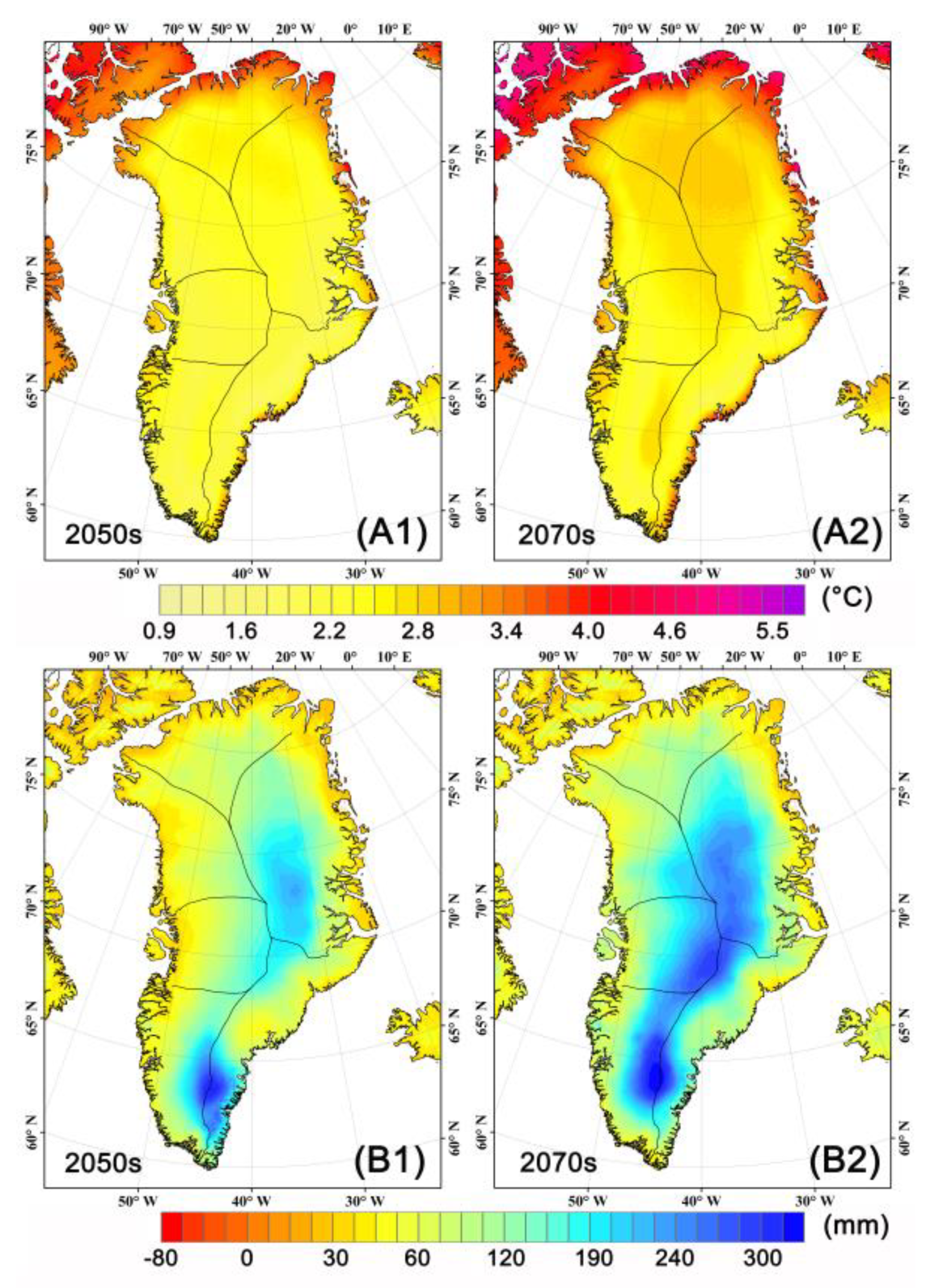
Modeled climate data based on the RCP4.5 climate scenario were selected to simulate Greenland’s increase in average annual temperature by the year 2050 (A1) and 2070 (A2) and the average yearly temperature by 2050s (B1) and 2070 (B2) and the increase in precipitation compared to 2010s (Figure 6). The CCSM4 simulations under a climate change scenario show that larger temperature increases appear in the northern portions of Greenland, which is consistent with the rising trend observed since the 20th century [54]. By the 2070s, Greenland will face more obvious warming, and the warming range will be more than 4 °C compared with the 2010s. By the 2050s, precipitation may be as high as 300 mm yr−1. The area of increased precipitation will be located in the central and eastern Greenland and the southeast region. The surrounding coastal area is also an area with increased precipitation, but the degree is weaker than the former.
4. Discussion
4.1. Error Analysis
In recent years, there have been many studies on the mass balance of mass changes in the Greenland Ice Sheet. Table 1 compares the results of this study with other selected research results, summarizing recent estimates of mass loss and corresponding sea-level rise. The results vary greatly, mainly due to the use of linear trends at different time intervals; the use of this trend is not suitable for longer time series, because interdecadal changes in climate and ocean temperature will change the ice sheet.
The Greenland Ice Sheet mass changes obtained in this study show two stages: a positive mass accumulation from 2002 to 2006 and a mass ablation from 2007 to 2019. The mass accumulation of the Greenland Ice Sheet over 2002–2006 exceeded 3.7 × 10³ Gt, and the mass change rate was about −126.35 Gt yr−1. The total ablation of the Greenland Ice Sheet analyzed in this study during 2007–2019 exceeded 28.9 × 10³ Gt, and the mass change rate was about 277.61 Gt yr−1. During the entire study period, the Greenland Ice Sheet mass change rate was −263.97 Gt yr−1, and the regional study interval error was 13.676 Gt yr−1. Three sets of Greenland global mass ablation results were selected as a reference. Based on the GRACE gravity model processed from Centre National d’Etudes Spatiales (CNES), Center of Space Research (CSR), and Geo Forschungs Zentrum (GFZ) from the first half of 2002 to the second half of 2007, Slobbe et al. estimated the mass change rate of Greenland to be between −128 Gt yr−1 and −218 Gt yr−1 [45]. During the same period, Zou et al. (2016) studied the changes of glaciers in Greenland through GRACE and ICESat, showing that the rate of ice change from January 2003 to June 2007 was −142.14 Gt yr−1, and the total ice loss estimated from ICESat during the same period was 173.03 Gt yr−1 [59]. The Greenland Ice Sheet mass balance estimate obtained by the IMBIE team from satellite altimetry, gravimetry, and input–output methods peaked at 275 ± 28 Gt yr−1 from 2007 to 2012. Its mass change rate in 2012 and 2017 was −244 ± 28 Gt yr−1 [24]. Compared with the three studies, the error range of this paper is 1.65–46.68 Gt yr−1, which falls within the allowable range.
On a regional scale, there was a mass loss in the SW and SE. The average mass change rates from 2002 to 2019 were −79.591 Gt yr−1 and −69.631 Gt yr−1. In the NE and CW, the annual average mass change rate were −59.796 Gt yr−1 and −54.987 Gt yr−1, respectively. The areas that had relatively weak mass changes were N and NW. The mass change rate here was −26.87 Gt yr−1 and −4.099 Gt yr−1. The partition error was maintained at 8.80–5.95 Gt yr−1.
In general, the biggest error in the GRACE products is the presence of correlated error. This manifests itself as north–south stripes due to poor observability of the east–west component of the gravity gradient. Secondly, they are limited by the greater uncertainty of the glacier isostatic pressure adjustment (GIA) model (Wahr et al., 1998) Although the clutter removal is very effective, especially for larger spatial scales, it will also remove some real geophysical signals and stripes. The size, shape, and direction of the signal strongly affect the effectiveness of clutter removal [60,61].
Adjusting the gravity solution can be used as an alternative to an empirical post-processing filter used to eliminate related errors, so that the related errors are suppressed during data inversion, thereby effectively eliminating the need for post-processing. Many recent studies have used the mascon basis function, using a nearly global set of geophysical models and auxiliary remote sensing observations to adjust the solution in the Bayesian method to suppress the relevant errors in the gravity inversion process [30]. The filter is allowed to adjust all estimated parameters at the same time, including not only the basic functions that define the earth’s gravity field, but also satellite status, accelerometer bias, scale factors, and any other harmful parameters. These adjustments greatly improve the accuracy of the data.
4.2. Summary
The Greenland Ice Sheet may continue to lose mass as a consequence of climate change; the speed of future loss is not necessarily less than that observed in the past decade. Extreme weather responses cannot be ruled out, which in turn may lead to a higher rate of mass loss [54]. Predicted climate scenarios show that the central region may become affected by severe climate change in the future. In addition, since the ice sheet surface balance is generally determined by the amount of precipitation and surface energy balance, more attention is needed to predict the change in precipitation [62]. This also indicates that not only the coastal region of Greenland is facing a serious mass ablation trend, but the seemingly stable central and northern areas will also face the same declines in the future. This is consistent with Moon’s research, which noted that in the late 20th-century mass losses across the Arctic began to accelerate; it is expected that losses will continue to be consistent across all future greenhouse gas emissions scenarios [63]. Secondly, between the end of the 20th century and the beginning of the 21st century, northern Greenland and lower elevations areas experienced the largest increases in temperature; in the future, the temperature increase in the northern high latitudes may still be the most dramatic, indicating that mass change is will need more attention [64].
Various researchers hold different views explaining the mass change of the Greenland Ice Sheet. Some view that the increase in temperature and the decrease in the surface albedo are the direct causes of the mass change of the ice sheet [65]. Rajewicz et al. (2014) attributed 38–49% of the changes in Greenland summer temperature and melting degree to the circulation anomaly, and the background warming of the lower troposphere explained 13–27% [66]. Others believe that the mass loss of the ice sheet was due to the surface increased melting and explained it with the accelerated termination of the glaciers at the exit of the ocean [67,68]. This also explains the increase in temperature and the increase in the melting of the seabed, which caused the withdrawal of the glaciers ending in the oceans. The fluctuation of the snow line at a higher altitude also exerts a more significant control on the mass change of the ice sheet. The explanations for the differences in the temporal and spatial variations of the Greenland Ice Sheet include the number of glaciers in each region and the depth of the glaciers. The glaciers with deeper ground lines may have greater mass loss [69,70,71,72]. This article compared the changes in ice sheet mass with climate data. It concludes that the two show a related change trend in time. It can be considered that the change in ice sheet mass is a response to the continuous warming of the climate to a certain extent. With future climate changes the Greenland Ice Sheet may face an accelerated loss trend.
5. Conclusions
This paper used GRACE Level-2 RL06 gravity field data from April 2002 to September 2019, and the Mascon scheme to obtain time series of Greenland Ice Sheet mass changes. The least-square method was used to analyze the Greenland Ice Sheet. The research shows that: (i) From April 2002 to September 2019, the total mass reduction rate of the Greenland Ice Sheet was about −263 ± 13 Gt yr−1; the acceleration was −41 ± 1.89 Gt yr−1, with a substantial regional difference. In the study interval, the area of ice sheet ablation was mainly concentrated in the marginal area, while in the central area, the mass of the ice sheet increased first and then decreased. (ii) Among the six watersheds considered, SW, SE, NW, and CW had a faster rate of mass decrease of −79.591 Gt yr−1, −69.631 Gt yr−1, −59.796 Gt yr−1, −54.987 Gt yr−1 and −26.87 Gt yr−1, respectively. Only the N watershed had a relatively balanced mass change, with an ablation rate of −4.099 Gt yr−1. The main reason for this difference is that the coastal area is the most common and significant area in Greenland where ice and snow interact with the ocean. A large number of glaciers with high flow velocity are mainly concentrated in the coastal areas, causing a large amount of outflow to be injected into the ocean. (iii) The analysis of climate change during the same period showed that Greenland’s temperature and precipitation have increased correspondingly. Compared with the 1990s, the increases of the 2010s are −0.4~3 °C yr−1, and −300~400 mm yr−1. Based on the RCP4.5 climate scenario prediction, the increase in temperature and precipitation in the 2050s are expected to further increase and, to a certain extent, to accelerate the melting of the Greenland Ice Sheet. In general, the results from other studies based on GRACE data show large differences, and the main reason is that their observation times are not in agreement. The observation period with GRACE data used in this study was longer. The rate of mass change of the Greenland Ice Sheet increase has resulted in a deviation from other GRACE results, but is still within the allowable error range.
Author Contributions
Y.M. carried out the main data search, processing, and paper writing work, Y.W. proposed the paper ideas and participated in the data processing, J.W. carried out the paper revision work, and Y.D., D.S. and D.Z. gave valuable comments in the paper writing and helped to collect and check the data. All authors have read and agreed to the published version of the manuscript.
Funding
The research is supported by the Strategic Priority Research Program of the Chinese Academy of Sciences (Grant No. XDA19070501 and XDA23060702), China National Natural Science Foundation (No.41771084, 41730751). We are very grateful for their generous funding.
Conflicts of Interest
The authors declare no conflict of interest.
References
- Cazenave, A.; Remy, F. Sea level and climate: Measurements and causes of changes. Wires Clim. Chang. 2011, 2, 647–662. [Google Scholar] [CrossRef]
- Reddy, S.J. Comments on IPCC’s 24th September 2019 Report on “The Ocean and Cryosphere in a Changing Climate: Summary for Policy Makers”. Acta Sci. Agric. 2019, 3, 16–19. [Google Scholar] [CrossRef]
- IPCC. Special Report on the Ocean and Cryosphere in a Changing Climate; Pörtner, H.-O., Roberts, D.C., Masson-Delmotte, V., Zhai, P., Eds.; Cambridge University Press: Cambridge, UK, 2019. [Google Scholar]
- Comiso, J.C.; Parkinson, C.L. Satellite-Observed Changes in the Arctic. Phys. Today 2004, 57, 38–44. [Google Scholar] [CrossRef] [Green Version]
- Andersen, M.L.; Stenseng, L.; Skourup, H.; Colgan, W.; Khan, S.A.; Kristensen, S.S.; Andersen, S.B.; Box, J.E.; Ahlstrøm, A.P.; Fettweis, X.; et al. Basin-scale partitioning of Greenland ice sheet mass balance components (2007–2011). Earth Planet. Sci. Lett. 2015, 409, 89–95. [Google Scholar] [CrossRef]
- Andrews, L.C. Greenland’s subglacial methane released. Nature 2019, 565, 31–32. [Google Scholar] [CrossRef] [Green Version]
- Morlighem, M.; Williams, C.N.; Rignot, E.; An, L.; Arndt, J.E.; Bamber, J.L.; Catania, G.; Chauche, N.; Dowdeswell, J.A.; Dorschel, B.; et al. BedMachine v3: Complete Bed Topography and Ocean Bathymetry Mapping of Greenland From Multibeam Echo Sounding Combined With Mass Conservation. Geophys. Res. Lett. 2017, 44, 11051–11061. [Google Scholar] [CrossRef] [Green Version]
- Stocker, T.; Qin, D.; Plattner, G.; Tignor, M.; Allen, S.; Boschung, J.; Nauels, A.; Xia, Y.; Bex, V.; Midgley, P. IPCC 2013: Summary for Policymakers. In Climate Change 2013: The Physical Science Basis, Contribution of Working Group I to the Fifth Assessment Report of the Intergovernmental Panel on Climate Change; Cambridge University Press: Cambridge, UK; New York, NY, USA, 2013. [Google Scholar]
- Qin, D.H.; Ding, Y.J.; Xiao, C.D.; Kang, S.; Ren, J.; Yang, J.; Zhang, S. Cryospheric Science: Research framework and disciplinary system. Natl. Sci. Rev. 2017, 5, 255–268. [Google Scholar] [CrossRef] [Green Version]
- Boncori, J.P.M.; Andersen, M.L.; Dall, J.; Kusk, A.; Kamstra, M.; Andersen, S.B.; Bechor, N.; Bevan, S.; Bignami, C.; Gourmelen, N.; et al. Intercomparison and Validation of SAR-Based Ice Velocity Measurement Techniques within the Greenland Ice Sheet CCI Project. Remote Sens. 2018, 10, 929. [Google Scholar] [CrossRef] [Green Version]
- Felikson, D.; Urban, T.J.; Gunter, B.C.; Pie, N.; Pritchard, H.D.; Harpold, R.; Schutz, B.E. Comparison of Elevation Change Detection Methods from ICESat Altimetry Over the Greenland Ice Sheet. IEEE Trans. Geosci. Remote Sens. 2017, 55, 5494–5505. [Google Scholar] [CrossRef]
- Webb, C.E.; Jay, Z.H.; Abdalati, W. The Ice, Cloud, and land Elevation Satellite (ICESat) Summary Mission Timeline and Performance Relative to Pre-Launch Mission Success Criteria; GSFC-E-DAA-TN6105; NASA: Washington, DC, USA, 2012.
- Abdalati, W.; Zwally, H.J.; Bindschadler, R.; Csatho, B.; Farrell, S.L.; Fricker, H.A.; Harding, D.; Kwok, R.; Lefsky, M.; Markus, T.; et al. The ICESat-2 Laser Altimetry Mission. Proc. IEEE 2010, 98, 735–751. [Google Scholar] [CrossRef]
- Zlotnicki, V.; Bettadpur, S.; Landerer, F.W.; Watkins, M.M. Gravity Recovery and Climate Experiment (GRACE): Detection of Ice Mass Loss, Terrestrial Mass Changes, and Ocean Mass Gains. In Encyclopedia of Sustainability Science and Technology; Meyers, R.A., Ed.; Springer: New York, NY, USA, 2012. [Google Scholar]
- Khan, S.; Wahr, J.; Stearns, L.; Hamilton, G.; Van Dam, T.; Larson, K.; Francis, O. Elastic uplift southeast Greenland due to rapid ice mass loss. Geophys. Res. Lett. 2007, 34. [Google Scholar] [CrossRef] [Green Version]
- Ramillien, G.; Lombard, A.; Cazenave, A.; Ivins, E.R.; Llubes, M.; Remy, F.; Biancale, R. Interannual variations of the mass balance of the Antarctica and Greenland ice sheets from GRACE. Glob. Planet. Chang. 2006, 53, 198–208. [Google Scholar] [CrossRef]
- Velicogna, I.; Mohajerani, Y.; Geruo, A.; Landerer, F.; Mouginot, J.; Noel, B.; Rignot, E.; Sutterley, T.; van den Broeke, M.; van Wessem, M.; et al. Continuity of Ice Sheet Mass Loss in Greenland and Antarctica From the GRACE and GRACE Follow-On Missions. Geophys. Res. Lett. 2020, 47. [Google Scholar] [CrossRef] [Green Version]
- Tapley, B.D.; Watkins, M.M.; Flechtner, F.; Reigber, C.; Bettadpur, S.; Rodell, M.; Sasgen, I.; Famiglietti, J.S.; Landerer, F.W.; Chambers, D.P.; et al. Contributions of GRACE to understanding climate change. Nat. Clim. Chang. 2019, 5, 358–369. [Google Scholar] [CrossRef]
- Wouters, B.; Chambers, D.; Schrama, E.J.O. GRACE observes small-scale mass loss in Greenland. Geophys. Res. Lett. 2008, 35. [Google Scholar] [CrossRef] [Green Version]
- Baur, O.; Kuhn, M.; Featherstone, W.E. GRACE-derived ice-mass variations over Greenland by accounting for leakage effects. J. Geophys. Res. 2009, 114. [Google Scholar] [CrossRef] [Green Version]
- Christoffersen, P. Greenland Ice Sheet. In Encyclopedia of Snow, Ice and Glaciers. Encyclopedia of Earth Sciences Series; Singh, V.P., Singh, P., Haritashya, U.K., Eds.; Springer: Dordrecht, The Netherlands, 2011; 1253p. [Google Scholar]
- Porter, C.; Morin, P.; Howat, I.; Noh, M.; Bates, B.; Peterman, K.; Keesey, S.; Schlenk, M.; Gardiner, J.; Tomko, K.; et al. ArcticDEM; Harvard Dataverse, V1; Harvard: Cambridge, MA, USA, 2018. [Google Scholar] [CrossRef]
- Rignot, E.; Velicogna, I.; van den Broeke, M.R.; Monaghan, A.; Lenaerts, J.T.M. Acceleration of the contribution of the Greenland and Antarctic ice sheets to sea level rise. Geophys. Res. Lett. 2011, 38. [Google Scholar] [CrossRef] [Green Version]
- Physical Oceanography Distributed Active Archive Center (PO.DAAC). Available online: https://podaac.jpl.nasa.gov/datasetlist?ids=ProcessingLevel:Collections&values=*3*:GRACE%20RL06&search=GRACE&view=list (accessed on 6 November 2019).
- Rignot, E.; Mouginot, J. Ice flow in Greenland for the International Polar Year 2008–2009. Geophys. Res. Lett. 2012, 39. [Google Scholar] [CrossRef] [Green Version]
- Shepherd, A.; Ivins, E.; Rignot, E.; Smith, B.; van den Broeke, M.; Velicogna, I.; Whitehouse, P.; Briggs, K.; Joughin, I.; Krinner, G.; et al. Mass balance of the Greenland Ice Sheet from 1992 to 2018. Nature 2020, 579, 233–239. [Google Scholar]
- Van Angelen, J.H.; van den Broeke, M.R.; Wouters, B.; Lenaerts, J.T.M. Contemporary (1960–2012) Evolution of the Climate and Surface Mass Balance of the Greenland Ice Sheet. Surv. Geophys. 2013, 35, 1155–1174. [Google Scholar] [CrossRef] [Green Version]
- Wiese, D.N.; Yuan, D.-N.; Boening, C.; Landerer, F.W.; Watkins, M.M. JPL GRACE Mascon Ocean, Ice, and Hydrology Equivalent Water Height Release 06 Coastal Resolution Improvement (CRI) Filtered Version1.0.; Version 1.0. PO.DAAC; PO.DAAC: Pasadena, CA, USA, 2018. Available online: http://0-dx-doi-org.brum.beds.ac.uk/10.5067/TEMSC-3MJC6 (accessed on 20 July 2020).
- Landerer, F.W.; Flechtner, F.M.; Save, H.; Webb, F.H.; Bandikova, T.; Bertiger, W.I.; Bettadpur, S.V.; Byun, S.H.; Dahle, C.; Dobslaw, H.; et al. Extending the Global Mass Change Data Record: GRACE Follow-On Instrument and Science Data Performance. Geophys. Res. Lett. 2020, 47, e2020GL088306. [Google Scholar] [CrossRef]
- Watkins, M.M.; Wiese, D.N.; Yuan, D.-N.; Boening, C.; Landerer, F.W. Improved methods for observing Earth’s time variable mass distribution with GRACE using spherical cap mascons. J. Geophys. Res. Solid Earth 2015, 120, 2648–2671. [Google Scholar] [CrossRef]
- Wiese, D.N.; Landerer, F.W.; Watkins, M.M. Quantifying and reducing leakage errors in the JPL RL05M GRACE mascon solution. Water Resour. Res. 2016, 52, 7490–7502. [Google Scholar] [CrossRef]
- Cheng, M.; Tapley, B.D. Variations in the Earth’s oblateness during the past 28 years. J. Geophys. Res. Solid Earth 2004, 109. [Google Scholar] [CrossRef]
- Purcell, A.; Tregoning, P.; Dehecq, A. An assessment of the ICE6G_C(VM5a) glacial isostatic adjustment model. J. Geophys. Res. Solid Earth 2016, 121, 3939–3950. [Google Scholar] [CrossRef] [Green Version]
- Peltier, W.R. Global Glacial Isostasy and the Surface of the Ice-Age Earth: The ICE-5G(VM2). model and GRACE. Ann. Rev. Earth Planet. Sci. 2004, 32, 111–149. [Google Scholar] [CrossRef]
- Geruo, A.; Wahr, J.M.; Zhong, S. Computations of the viscoelastic response of a 3-D compressible Earth to surface loading: An application to Glacial Isostatic Adjustment in Antarctica and Canada. Geophys. J. Int. 2012, 192, 557–572. [Google Scholar] [CrossRef]
- WorldClim. Available online: http://worldclim.org (accessed on 18 April 2020).
- University of East Anglia Climatic Research Unit; Harris, I.C.; Jones, P.D. CRU TS4.03: Climatic Research Unit (CRU) Time-Series (TS) Version 4.03 of High-Resolution Gridded Data of Month-by-Month Variation in Climate (Jan. 1901–Dec. 2018); Centre for Environmental Data Analysis (CEDA): Chilton, WI, USA, 2020. [Google Scholar]
- Fick, S.E.; Hijmans, R.J. WorldClim 2: New 1-km spatial resolution climate surfaces for global land areas. Int. J. Clim. 2017, 37, 4302–4315. [Google Scholar] [CrossRef]
- Velicogna, I.; Wahr, J. Greenland mass balance from GRACE. Geophys. Res. Lett. 2005, 32. [Google Scholar] [CrossRef] [Green Version]
- Jacob, T.; Wahr, J.; Pfeffer, W.T.; Swenson, S. Recent contributions of glaciers and ice caps to sea level rise. Nature 2012, 482, 514–518. [Google Scholar] [CrossRef]
- Luthcke, S.B.; Rowlands, D.D.; Lemoine, F.G.; Klosko, S.M.; Chinn, D.; McCarthy, J.J. Monthly spherical harmonic gravity field solutions determined from GRACE inter-satellite range-rate data alone. Geophys. Res. Lett. 2006, 33. [Google Scholar] [CrossRef]
- Ran, J.; Ditmar, P.; Klees, R.; Farahani, H.H. Statistically optimal estimation of Greenland Ice Sheet mass variations from GRACE monthly solutions using an improved mascon approach. J. Geod. 2018, 92, 299–319. [Google Scholar] [CrossRef] [PubMed] [Green Version]
- Baur, O.; Sneeuw, N. Assessing Greenland ice mass loss by means of point-mass modeling: A viable methodology. J. Geod. 2011, 85, 607–615. [Google Scholar] [CrossRef]
- Wahr, J.; Molenaar, M.; Bryan, F. Time variability of the Earth’s gravity field: Hydrological and oceanic effects and their possible detection using GRACE. J. Geophys. Res. Solid Earth 1998, 103, 30205–30229. [Google Scholar] [CrossRef]
- Slobbe, D.C.; Ditmar, P.; Lindenbergh, R.C. Estimating the rates of mass change, ice volume change and snow volume change in Greenland from ICESat and GRACE data. Geophys. J. Int. 2009, 176, 95–106. [Google Scholar] [CrossRef] [Green Version]
- Mote, T.L. Greenland surface melt trends 1973–2007: Evidence of a large increase in 2007. Geophys. Res. Lett. 2007, 34. [Google Scholar] [CrossRef]
- Catania, G.A.; Neumann, T.A.; Price, S.F. Characterizing englacial drainage in the ablation zone of the Greenland ice sheet. J. Glaciol. 2008, 54, 567–578. [Google Scholar] [CrossRef] [Green Version]
- Hanna, E.; Mernild, S.H.; Cappelen, J.; Steffen, K. Recent warming in Greenland in a long-term instrumental (1881–2012) climatic context: I. Evaluation of surface air temperature records. Env. Res. Lett. 2012, 7, 045404. [Google Scholar] [CrossRef]
- Diamond, M. Air Temperature and Precipitation on the Greenland Ice Sheet. J. Glaciol. 1960, 3, 558–567. [Google Scholar] [CrossRef] [Green Version]
- Berdahl, M.; Rennermalm, A.; Hammann, A.; Mioduszweski, J.; Hameed, S.; Tedesco, M.; Stroeve, J.; Mote, T.; Koyama, T.; McConnell, J.R. Southeast Greenland Winter Precipitation Strongly Linked to the Icelandic Low Position. J. Clim. 2018, 31, 4483–4500. [Google Scholar] [CrossRef]
- IPCC. Climate Change 2007: The Physical Science Basis; Solomon, S., Qin, D., Manning, M., Marquis, M., Averyt, K., Tignor, M.M.B., LeRoy Miller, H., Jr., Chen, Z., Eds.; Cambridge University Press: Cambridge, UK, 2007. [Google Scholar]
- Eisenman, I.; Untersteiner, N.; Wettlaufer, J.S. On the reliability of simulated Arctic sea ice in global climate models. Geophys. Res. Lett. 2007, 34. [Google Scholar] [CrossRef]
- Gorodetskaya, I.V.; Tremblay, L.B.; Liepert, B.; Cane, M.A.; Cullather, R.I. The Influence of Cloud and Surface Properties on the Arctic Ocean Shortwave Radiation Budget in Coupled Models. J. Clim. 2008, 21, 866–882. [Google Scholar] [CrossRef] [Green Version]
- Pattyn, F.; Ritz, C.; Hanna, E.; Asay-Davis, X.; DeConto, R.; Durand, G.; Favier, L.; Fettweis, X.; Goelzer, H.; Golledge, N.R.; et al. The Greenland and Antarctic ice sheets under 1.5 °C global warming. Nat. Clim. Chang. 2018, 8, 1053–1061. [Google Scholar] [CrossRef] [Green Version]
- Velicogna, I.; Wahr, J. Acceleration of Greenland ice mass loss in spring 2004. Nature 2006, 443, 329–331. [Google Scholar] [CrossRef] [PubMed] [Green Version]
- Ran, J.; Vizcaino, M.; Ditmar, P.; van den Broeke, M.R.; Moon, T.; Steger, C.R.; Enderlin, E.M.; Wouters, B.; Noël, B.; Reijmer, C.H.; et al. Seasonal mass variations show timing and magnitude of meltwater storage in the Greenland Ice Sheet. Cryosphere 2018, 12, 2981–2999. [Google Scholar] [CrossRef] [Green Version]
- Forsberg, R.; Sørensen, L.; Simonsen, S. Greenland and Antarctica Ice Sheet Mass Changes and Effects on Global Sea Level. In Integrative Study of the Mean Sea Level and Its Components; Springer: Cham, Switzerland, 2017; pp. 91–106. [Google Scholar]
- Ewert, H.; Groh, A.; Dietrich, R. Volume and mass changes of the Greenland ice sheet inferred from ICESat and GRACE. J. Geodyn. 2012, 59–60, 111–123. [Google Scholar] [CrossRef]
- Zou, F.; Jin, S. Estimations of glacier melting in Greenland from combined satellite gravimetry and icesat. In Proceedings of the 2016 IEEE International Geoscience and Remote Sensing Symposium (IGARSS), Beijing, China, 10–15 July 2016; pp. 6185–6188. [Google Scholar]
- Wahr, J.; Swenson, S.; Velicogna, I. Accuracy of GRACE mass estimates. Geophys. Res. Lett. 2006, 33, 178–196. [Google Scholar] [CrossRef] [Green Version]
- Barrett, B.S.; Henderson, G.R.; McDonnell, E.; Henry, M.; Mote, T. Extreme Greenland blocking and high-latitude moisture transport. Atmos. Sci. Lett. 2020. [Google Scholar] [CrossRef]
- Golledge, N.R. Long-term projections of sea-level rise from ice sheets. Wires Clim. Chang. 2020, 11. [Google Scholar] [CrossRef]
- Moon, T.; Ahlstrom, A.; Goelzer, H.; Lipscomb, W.; Nowicki, S. Rising Oceans Guaranteed: Arctic Land Ice Loss and Sea Level Rise. Curr. Clim. Chang. Rep. 2018, 4, 211–222. [Google Scholar] [CrossRef] [Green Version]
- Lucas-Picher, P.; Wulff-Nielsen, M.; Christensen, J.H.; Aðalgeirsdóttir, G.; Mottram, R.; Simonsen, S.B. Very high resolution regional climate model simulations over Greenland: Identifying added value. J. Geophys. Res. Atmos. 2012, 117. [Google Scholar] [CrossRef] [Green Version]
- Hofer, S.; Tedstone, A.J.; Fettweis, X.; Bamber, J.L. Decreasing cloud cover drives the recent mass loss on the Greenland Ice Sheet. Sci. Adv. 2017, 3, e1700584. [Google Scholar] [CrossRef] [PubMed] [Green Version]
- Rajewicz, J.; Marshall, S.J. Variability and trends in anticyclonic circulation over the Greenland ice sheet, 1948–2013. Geophys. Res. Lett. 2014, 41, 2842–2850. [Google Scholar] [CrossRef]
- Beckmann, J. Modeling of Greenland outlet glaciers response to future climate change. In Proceedings of the AGU Fall Meeting, New Orleans, LA, USA, 11–15 December 2017. [Google Scholar]
- Charlie, B.; Rachel, C.J.; Nienow, P.W.; Ross, N.; Killick, R. Ice front change of marine-terminating outlet glaciers in northwest and southeast Greenland during the 21st century. J. Glaciol. 2018, 64, 523–535. [Google Scholar]
- Straneo, F.; Heimbach, P. North Atlantic warming and the retreat of Greenland’s outlet glaciers. Nature 2013, 504, 36–43. [Google Scholar] [CrossRef] [PubMed]
- Ryan, J.C.; Smith, L.C.; van As, D.; Cooley, S.W.; Cooper, M.G.; Pitcher, L.H.; Hubbard, A. Greenland Ice Sheet surface melt amplified by snowline migration and bare ice exposure. Sci. Adv. 2019, 5, eaav3738. [Google Scholar] [CrossRef] [PubMed] [Green Version]
- Boghosian, A.; Porter, D.F.; Tinto, K.J.; Bell, R.E.; Cochran, J.R.; Csatho, B.M. New Gravity-Derived Grounding Line Depths Highlight Role Bathymetry Plays in Ongoing Greenland Ice Sheet Change. In Proceedings of the AGU Fall Meeting, San Francisco, CA, USA, 15–19 December 2014. [Google Scholar]
- Nagler, T.; Rott, H.; Hetzenecker, M.; Wuite, J.; Potin, P. The Sentinel-1 Mission: New Opportunities for Ice Sheet Observations. Remote Sens. 2015, 7, 9371–9389. [Google Scholar] [CrossRef] [Green Version]
Figure 1.
Greenland regions superimposed on the elevation map.

Figure 2.
The rate of change of Greenland Ice Sheet mass variations (in Equivalent Water Thickness cm/yr).
Figure 2.
The rate of change of Greenland Ice Sheet mass variations (in Equivalent Water Thickness cm/yr).

Figure 3.
Greenland’s total mass trends from 2002 to 2019 and mass change rate.

Figure 4.
Greenland’s mass change in different watersheds from 2002 to 2019.

Figure 5.
The difference annual mean temperature of Greenland between two time periods (A1) and (A2), and the annual difference precipitation of Greenland two time periods (B1) and (B2), were generated from the differences between the two periods 1990s and 2010s (Mean T/P2011-2018 minus Mean T/P1991-2000) based on the Climatic Research Unit (CRU) TS4.03 dataset (https://catalogue.ceda.ac.uk/).

Figure 6.
The different increases of annual mean temperature of Greenland under the RCP4.5 in the 2050s (A1) and 2070s (A2), and the projected increases of annual precipitation of Greenland under the RCP4.5 in 2050s (B1) and 2070s (B2), were generated from the differences between the two periods 2050s and 2070s to present 2010s (Mean T/P2041-2050 or T/P2061-2070 minus Mean T/P2001-2010) based on Coupled Model Inter-comparison Project version 5 (CMIP5) Community Climate System Model (CCSM) Version 4 (CCSM4) dataset (http://worldclim.org/) with a spatial resolution of 30 s.


Table 1.
Comparison of estimated mass change trends in Greenland.
| Period | Literature | Date | Rate of Mass Change(Gt yr−1) | Tolerance Scope(−/+) |
|---|---|---|---|---|
| 2002~2005 | Ramillien et al. [17] | GRACE | 107 | 23 |
| 2002~2006 | Velicogna et al. [55] | GRACE | 223.33 | 36 |
| 2003~2007 | Slobbe et al. [45] | ICESat | 139 | 68 |
| 2002~2007 | Slobbe et al. [45] | GRACE | 128~218 | 90 |
| 2003~2008 | Woters et al. [20] | GRACE(CSR) | 179 | 25 |
| 2002~2008 | Baur et al. [21] | GRACE | 177 | 12 |
| 2007~2012 | Shepherd et al. [27] | 26 Satellites | 275 | 28 |
| 2012~2017 | Shepherd et al. [27] | 26 Satellites | 244 | 28 |
| 2003~2012 | Ran et al. [56] | RACMO/GRACE | 216 | 122 |
| 2003~2013 | Ran et al. [56] | GRACE | 286 | 21 |
| 2002~2015 | Forsberg et al. [57] | GRACE | 265 | 25 |
| 2002~2009 | Ewert et al. [58] | GRACE(GFZ) | 191.21 | 20.9 |
| 2002~2019 | This article | GRACE | 263.97 | 13 |
© 2020 by the authors. Licensee MDPI, Basel, Switzerland. This article is an open access article distributed under the terms and conditions of the Creative Commons Attribution (CC BY) license (http://creativecommons.org/licenses/by/4.0/).
Share and Cite
MDPI and ACS Style
Mu, Y.; Wei, Y.; Wu, J.; Ding, Y.; Shangguan, D.; Zeng, D. Variations of Mass Balance of the Greenland Ice Sheet from 2002 to 2019. Remote Sens. 2020, 12, 2609. https://0-doi-org.brum.beds.ac.uk/10.3390/rs12162609
AMA Style
Mu Y, Wei Y, Wu J, Ding Y, Shangguan D, Zeng D. Variations of Mass Balance of the Greenland Ice Sheet from 2002 to 2019. Remote Sensing. 2020; 12(16):2609. https://0-doi-org.brum.beds.ac.uk/10.3390/rs12162609
Chicago/Turabian StyleMu, Yaqiong, Yanqiang Wei, Jinkui Wu, Yongjian Ding, Donghui Shangguan, and Di Zeng. 2020. "Variations of Mass Balance of the Greenland Ice Sheet from 2002 to 2019" Remote Sensing 12, no. 16: 2609. https://0-doi-org.brum.beds.ac.uk/10.3390/rs12162609
Note that from the first issue of 2016, this journal uses article numbers instead of page numbers. See further details here.