A Multi-Sensor Unoccupied Aerial System Improves Characterization of Vegetation Composition and Canopy Properties in the Arctic Tundra

 , , , and
Abstract
:
1. Introduction
2. Materials and Methods
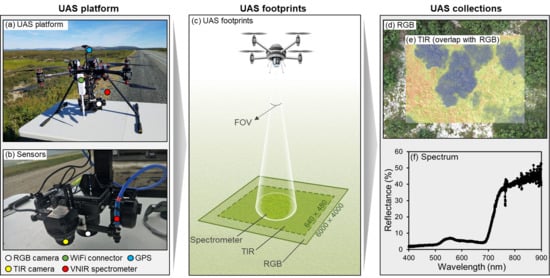
2.1. The Osprey Platform Setup
2.1.1. Airframe
2.1.2. Sensors
2.1.3. Software
2.2. Field Campaign
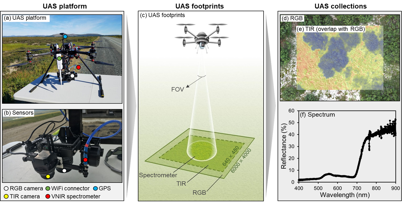
2.2.1. Study Site
2.2.2. Osprey Flights
2.2.3. Ground Measurements
2.3. Osprey Data Processing
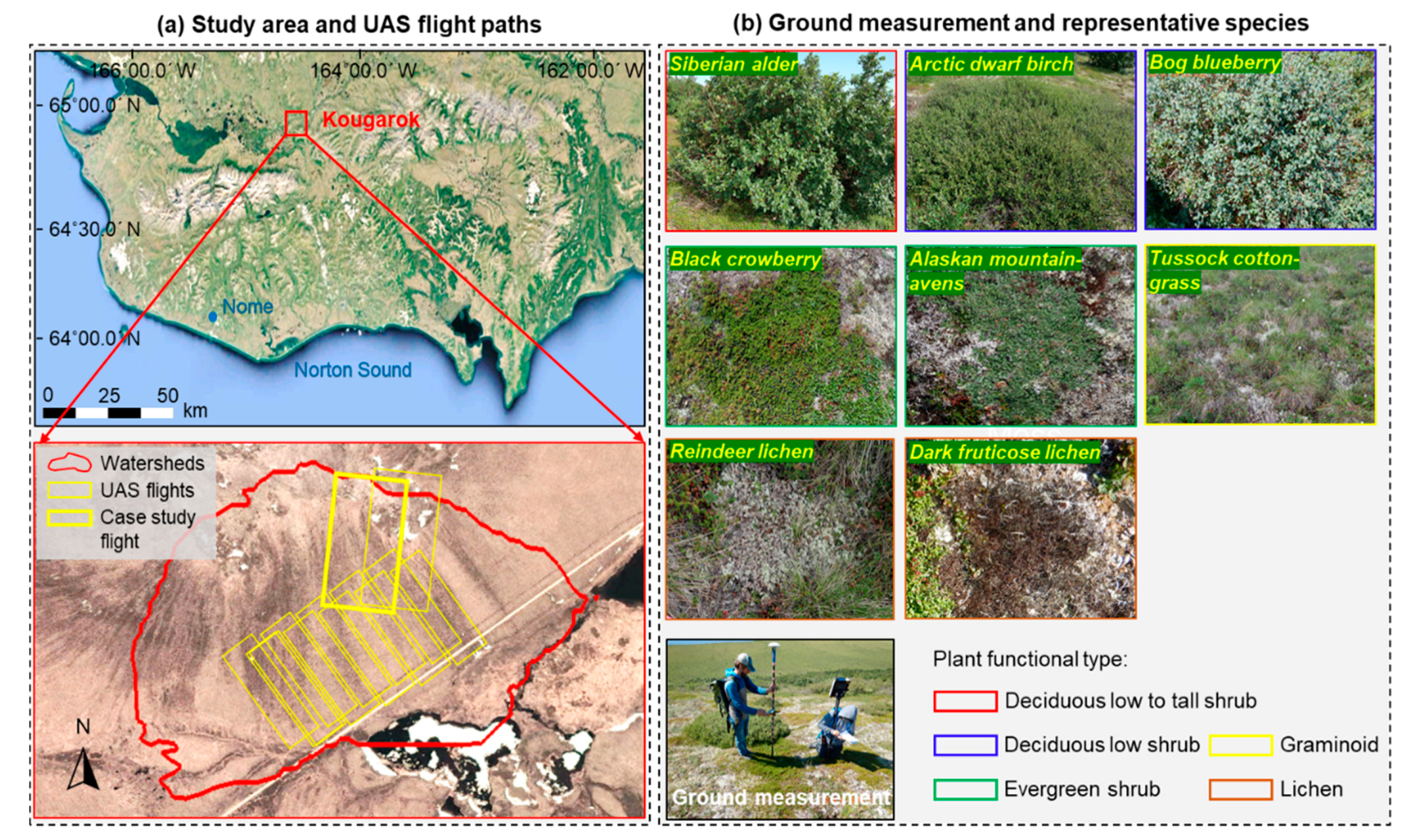
2.3.1. Processing the Osprey Raw Data Collections
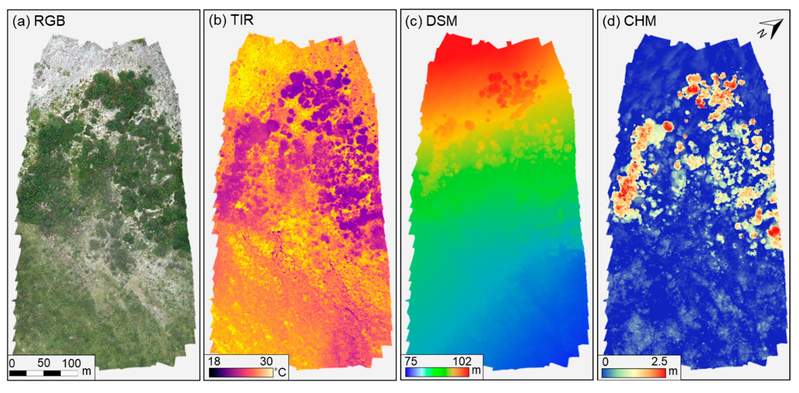
2.3.2. Deriving the Canopy Height Model (CHM)
- Identify ‘on-ground’ pixels from the DSM: We first performed an object-based classification on the four-band layer-stack of RGB and TIR (details for classification can be found in mapping tundra vegetation below). The ‘on-ground’ pixels were then identified as non-vegetation classes, e.g., schist rock and water, or non-vascular vegetation, e.g., lichen. By doing this, we avoided including any vegetation canopies that have a discernible height into the later reconstruction of the DEM, which serves as a base layer for deriving CHM.
- Interpolate the DEM using the ‘on-ground’ pixels: To produce a spatially continuous smooth DEM (i.e., without surface structure), we used a thin plate spline (TPS) algorithm [67] in ENVI+IDL to interpolate the ‘on-ground’ pixels. TPS provides smooth interpolation of given scattered data in two or more dimensions by considering geometric properties [68,69] and has been widely used for creating DEMs from LiDAR cloud points [70,71].
- Calculate the CHM: Once the DEM was obtained, we calculated the CHM by subtracting the DEM from the DSM. The resulting CHM has the same spatial resolution as the DSM.
2.4. Methods for the Case Study
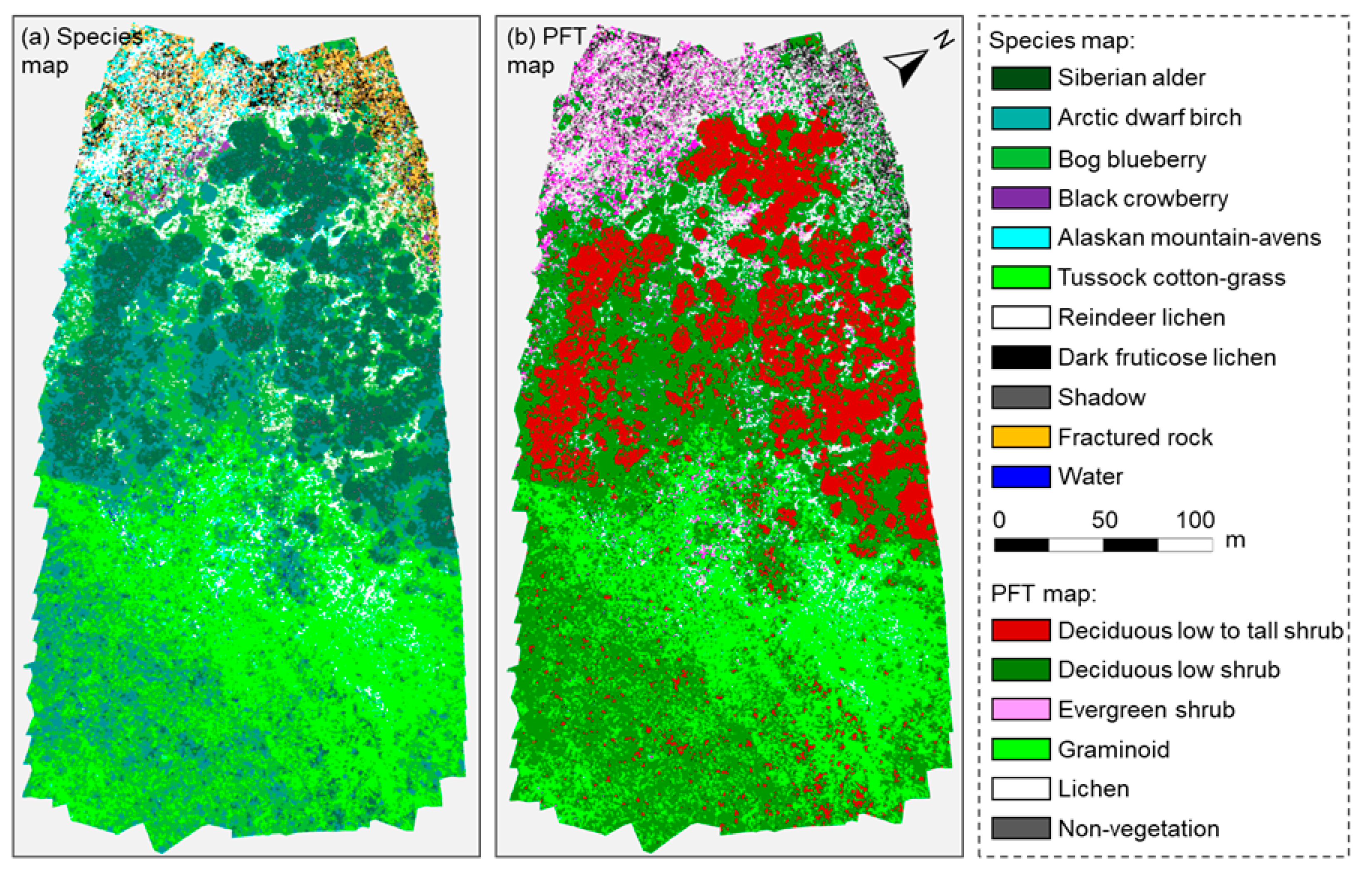
2.4.1. Mapping Tundra Vegetation
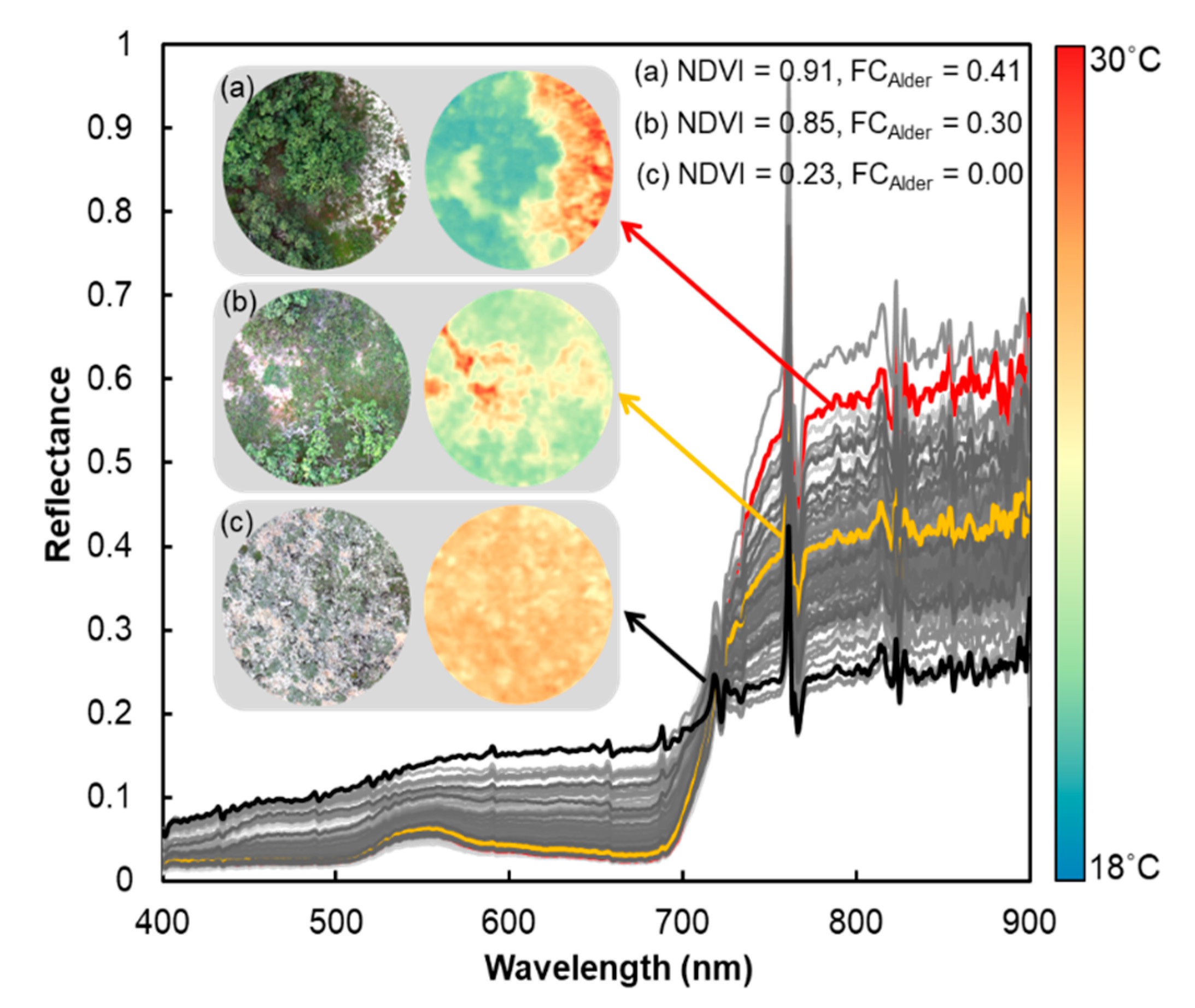
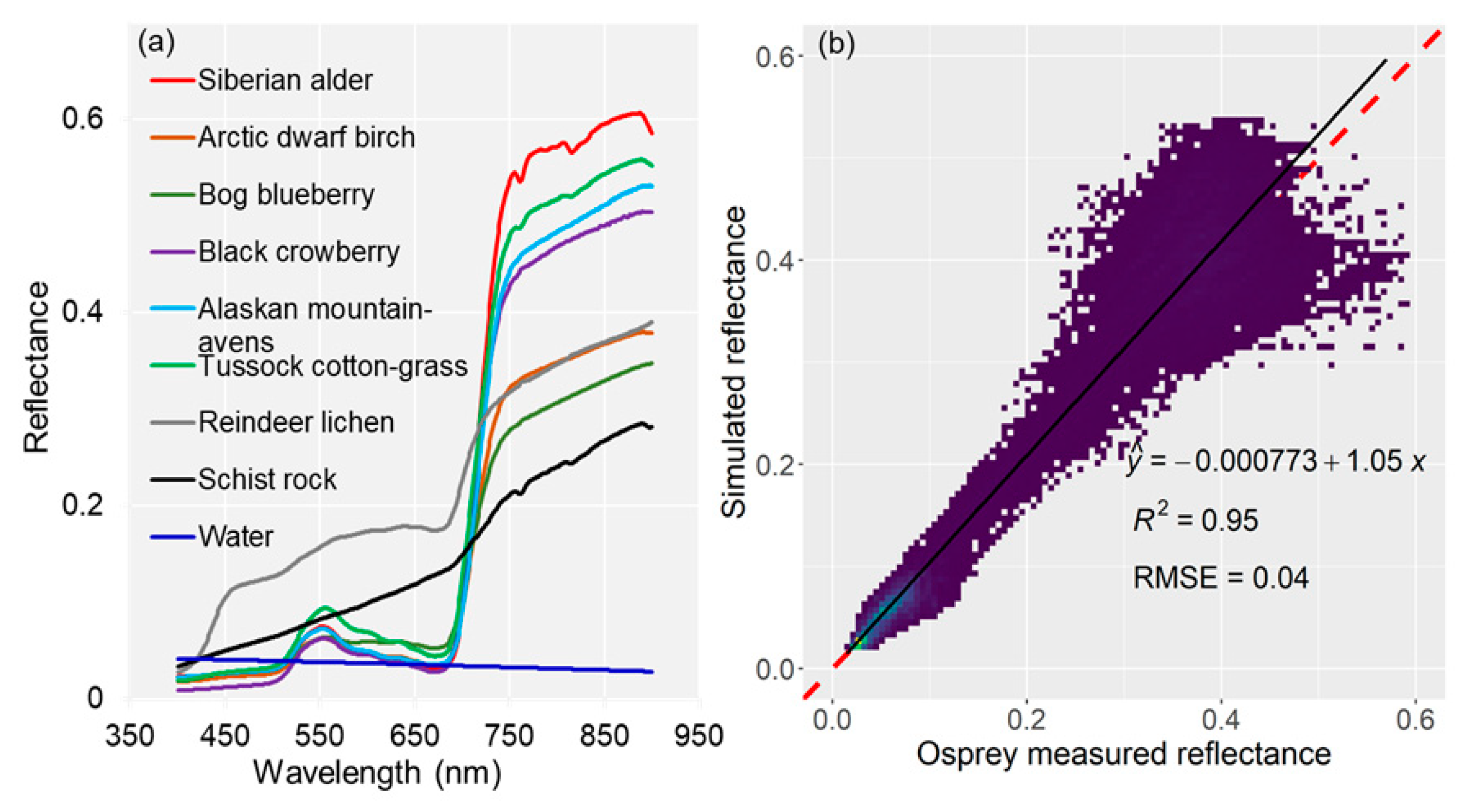
2.4.2. Evaluating Osprey Spectral Reflectance
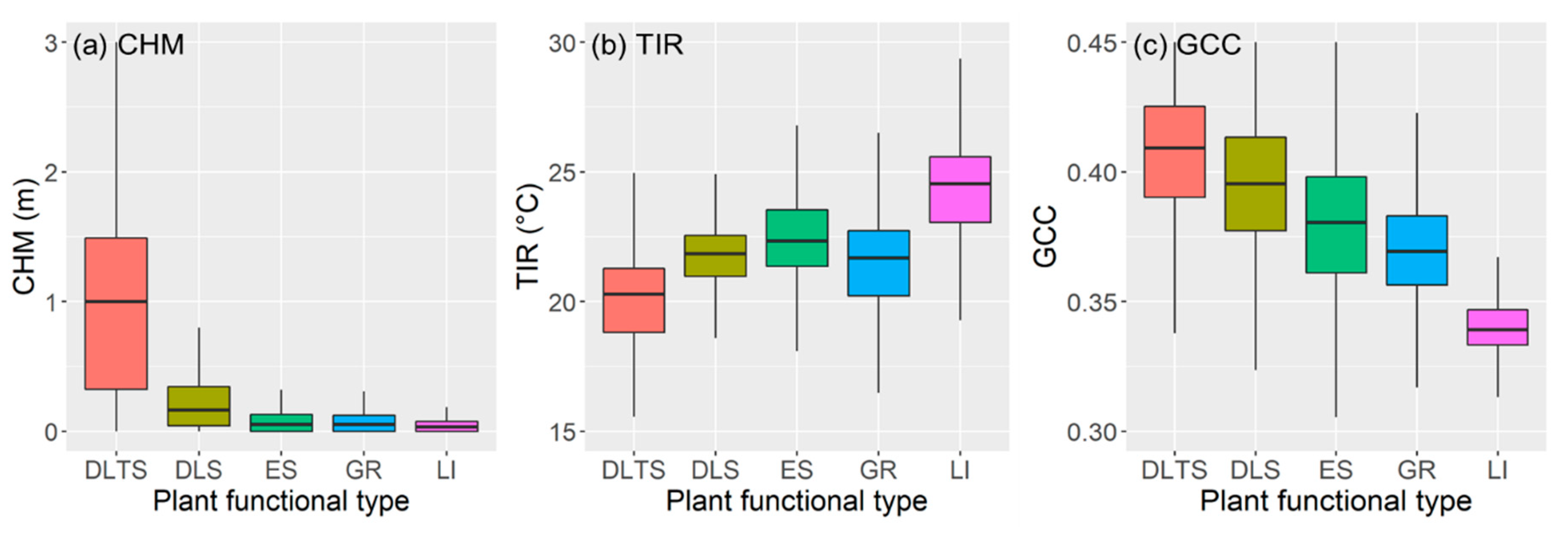
2.4.3. Characterizing Canopy Height, Temperature, and Greenness of PFTs
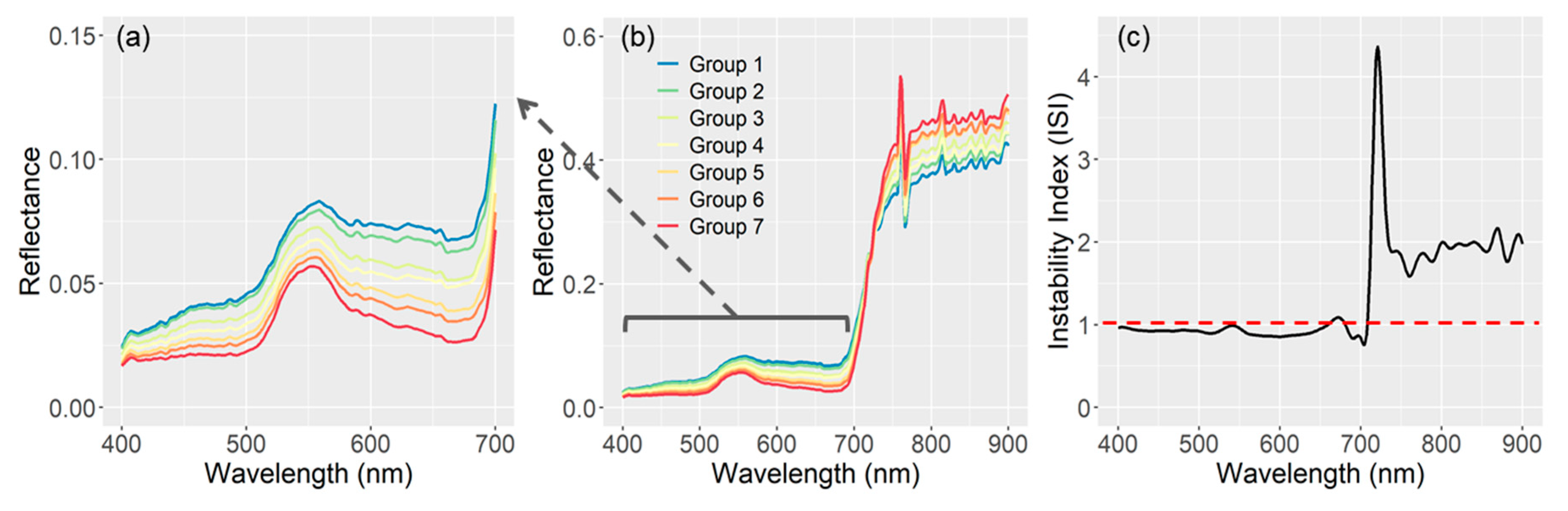
2.4.4. Quantifying Spectral Separability among Deciduous Low to Tall Shrub PFT Covers
3. Results
3.1. Osprey Image Products, Classification, and Canopy CHM, TIR, and GCC of Different PFTs
3.2. Osprey Spectra Products, Validation, and Spectral Separability among Deciduous Low to Tall Shrubs Covers
4. Discussion
5. Conclusions
Supplementary Materials
Author Contributions
Funding
Conflicts of Interest
References
- Post, E.; Forchhammer, M.C.; Bret-Harte, M.S.; Callaghan, T.V.; Christensen, T.R.; Elberling, B.; Fox, A.D.; Gilg, O.; Hik, D.S.; Høye, T.T.; et al. Ecological dynamics across the Arctic associated with recent climate change. Science 2009, 325, 1355–1358. [Google Scholar] [CrossRef] [Green Version]
- Elmendorf, S.C.; Henry, G.H.R.; Hollister, R.D.; Björk, R.G.; Boulanger-Lapointe, N.; Cooper, E.J.; Cornelissen, J.H.C.; Day, T.A.; Dorrepaal, E.; Elumeeva, T.G.; et al. Plot-scale evidence of tundra vegetation change and links to recent summer warming. Nat. Clim. Change 2012, 2, 453–457. [Google Scholar] [CrossRef]
- Schuur, E.A.G.; McGuire, A.D.; Schädel, C.; Grosse, G.; Harden, J.W.; Hayes, D.J.; Hugelius, G.; Koven, C.D.; Kuhry, P.; Lawrence, D.M.; et al. Climate change and the permafrost carbon feedback. Nature 2015, 520, 171–179. [Google Scholar] [CrossRef] [PubMed]
- Sturm, M.; Racine, C.; Tape, K. Increasing shrub abundance in the Arctic. Nature 2001, 411, 546–547. [Google Scholar] [CrossRef] [PubMed]
- Myers-Smith, I.H.; Forbes, B.C.; Wilmking, M.; Hallinger, M.; Lantz, T.; Blok, D.; Tape, K.D.; Macias-Fauria, M.; Sass-Klaassen, U.; Lévesque, E.; et al. Shrub expansion in tundra ecosystems: Dynamics, impacts and research priorities. Environ. Res. Lett. 2011, 6, 045509. [Google Scholar] [CrossRef] [Green Version]
- Tape, K.D.; Hallinger, M.; Welker, J.M.; Ruess, R.W. Landscape Heterogeneity of Shrub Expansion in Arctic Alaska. Ecosystems 2012, 15, 711–724. [Google Scholar] [CrossRef]
- Myneni, R.B.; Keeling, C.D.; Tucker, C.J.; Asrar, G.; Nemani, R.R. Increased plant growth in the northern high latitudes from 1981 to 1991. Nature 1997, 386, 698–702. [Google Scholar] [CrossRef]
- Ju, J.; Masek, J.G. The vegetation greenness trend in Canada and US Alaska from 1984–2012 Landsat data. Remote Sens. Environ. 2016, 176, 1–16. [Google Scholar] [CrossRef]
- Pearson, R.G.; Phillips, S.J.; Loranty, M.M.; Beck, P.S.A.; Damoulas, T.; Knight, S.J.; Goetz, S.J. Shifts in Arctic vegetation and associated feedbacks under climate change. Nat. Clim. Change 2013, 3, 673–677. [Google Scholar] [CrossRef]
- Callaghan, T.V.; Björn, L.O.; Chernov, Y.; Chapin, T.; Christensen, T.R.; Huntley, B.; Ims, R.A.; Johansson, M.; Jolly, D.; Jonasson, S.; et al. Effects on the Function of Arctic Ecosystems in the Short- and Long-term Perspectives. Ambio. J. Hum. Environ. 2004, 33, 448–458. [Google Scholar] [CrossRef]
- Juszak, I.; Iturrate-Garcia, M.; Gastellu-Etchegorry, J.-P.; Schaepman, M.E.; Maximov, T.C.; Schaepman-Strub, G. Drivers of shortwave radiation fluxes in Arctic tundra across scales. Remote Sens. Environ. 2017, 193, 86–102. [Google Scholar] [CrossRef] [Green Version]
- Myers-Smith, I.H.; Thomas, H.J.D.; Bjorkman, A.D. Plant traits inform predictions of tundra responses to global change. New Phytol. 2018, 221, 1742–1748. [Google Scholar] [CrossRef] [PubMed]
- Kokaly, R.F.; Despain, D.G.; Clark, R.N.; Livo, K.E. Mapping vegetation in Yellowstone National Park using spectral feature analysis of AVIRIS data. Remote Sens. Environ. 2003, 84, 437–456. [Google Scholar] [CrossRef] [Green Version]
- ASNER, G.; MARTIN, R. Spectral and chemical analysis of tropical forests: Scaling from leaf to canopy levels. Remote Sens. Environ. 2008, 112, 3958–3970. [Google Scholar] [CrossRef]
- Rossi, C.; Kneubühler, M.; Schütz, M.; Schaepman, M.E.; Haller, R.M.; Risch, A.C. From local to regional: Functional diversity in differently managed alpine grasslands. Remote Sens. Environ. 2020, 236, 111415. [Google Scholar] [CrossRef]
- Serbin, S.P.; Singh, A.; Desai, A.R.; Dubois, S.G.; Jablonski, A.D.; Kingdon, C.C.; Kruger, E.L.; Townsend, P.A. Remotely estimating photosynthetic capacity, and its response to temperature, in vegetation canopies using imaging spectroscopy. Remote Sens. Environ. 2015, 167, 78–87. [Google Scholar] [CrossRef]
- Jha, C.S.; Singhal, J.; Reddy, C.S.; Rajashekar, G.; Maity, S.; Patnaik, C.; Das, A.; Misra, A.; Singh, C.P.; Mohapatra, J.; et al. Characterization of Species Diversity and Forest Health using AVIRIS-NG Hyperspectral Remote Sensing Data. Curr. Sci. India 2019, 116, 1124–1135. [Google Scholar] [CrossRef]
- Chaube, N.R.; Lele, N.; Misra, A.; Murthy, T.V.R.; Manna, S.; Hazra, S.; Panda, M.; Samal, R.N. Mangrove Species Discrimination and Health Assessment using AVIRIS-NG Hyperspectral Data. Curr. Sci. India 2019, 116, 1136–1142. [Google Scholar] [CrossRef]
- Jucker, T.; Caspersen, J.; Chave, J.; Antin, C.; Barbier, N.; Bongers, F.; Dalponte, M.; van Ewijk, K.Y.; Forrester, D.I.; Haeni, M.; et al. Allometric equations for integrating remote sensing imagery into forest monitoring programmes. Glob. Change Biol. 2016, 23, 177–190. [Google Scholar] [CrossRef]
- Alonzo, M.; Andersen, H.-E.; Morton, D.; Cook, B. Quantifying Boreal Forest Structure and Composition Using UAV Structure from Motion. Forests 2018, 9, 119. [Google Scholar] [CrossRef] [Green Version]
- Alonzo, M.; Dial, R.J.; Schulz, B.K.; Andersen, H.-E.; Lewis-Clark, E.; Cook, B.D.; Morton, D.C. Mapping tall shrub biomass in Alaska at landscape scale using structure-from-motion photogrammetry and lidar. Remote Sens. Environ. 2020, 245, 111841. [Google Scholar] [CrossRef]
- Berni, J.; Zarco-Tejada, P.J.; Suarez, L.; Fereres, E. Thermal and Narrowband Multispectral Remote Sensing for Vegetation Monitoring From an Unmanned Aerial Vehicle. IEEE Trans Geosci. Remote 2009, 47, 722–738. [Google Scholar] [CrossRef] [Green Version]
- Zarco-Tejada, P.J.; González-Dugo, V.; Berni, J.A.J. Fluorescence, temperature and narrow-band indices acquired from a UAV platform for water stress detection using a micro-hyperspectral imager and a thermal camera. Remote Sens. Environ. 2012, 117, 322–337. [Google Scholar] [CrossRef]
- Stow, D.A.; Hope, A.; McGuire, D.; Verbyla, D.; Gamon, J.; Huemmrich, F.; Houston, S.; Racine, C.; Sturm, M.; Tape, K.; et al. Remote sensing of vegetation and land-cover change in Arctic Tundra Ecosystems. Remote Sens. Environ. 2004, 89, 281–308. [Google Scholar] [CrossRef] [Green Version]
- Laidler, G.J.; Treitz, P.M.; Atkinson, D.M. Remote Sensing of Arctic Vegetation: Relations between the NDVI, Spatial Resolution and Vegetation Cover on Boothia Peninsula, Nunavut. Arctic 2009, 61, 1–13. [Google Scholar] [CrossRef] [Green Version]
- Myers-Smith, I.H.; Kerby, J.T.; Phoenix, G.K.; Bjerke, J.W.; Epstein, H.E.; Assmann, J.J.; John, C.; Andreu-Hayles, L.; Angers-Blondin, S.; Beck, P.S.A.; et al. Complexity revealed in the greening of the Arctic. Nat. Clim. Change 2020, 10, 106–117. [Google Scholar] [CrossRef] [Green Version]
- Metcalfe, D.B.; Hermans, T.D.G.; Ahlstrand, J.; Becker, M.; Berggren, M.; Björk, R.G.; Björkman, M.P.; Blok, D.; Chaudhary, N.; Chisholm, C.; et al. Patchy field sampling biases understanding of climate change impacts across the Arctic. Nat. Ecol. Evol. 2018, 2, 1443–1448. [Google Scholar] [CrossRef]
- Riedel, S.M.; Epstein, H.E.; Walker, D.A. Biotic controls over spectral reflectance of arctic tundra vegetation. Int. J. Remote Sens. 2005, 26, 2391–2405. [Google Scholar] [CrossRef]
- Buchhorn, M.; Walker, D.; Heim, B.; Raynolds, M.; Epstein, H.; Schwieder, M. Ground-Based Hyperspectral Characterization of Alaska Tundra Vegetation along Environmental Gradients. Remote Sens. 2013, 5, 3971–4005. [Google Scholar] [CrossRef] [Green Version]
- Davidson, S.; Santos, M.; Sloan, V.; Watts, J.; Phoenix, G.; Oechel, W.; Zona, D. Mapping Arctic Tundra Vegetation Communities Using Field Spectroscopy and Multispectral Satellite Data in North Alaska, USA. Remote Sens. 2016, 8, 978. [Google Scholar] [CrossRef] [Green Version]
- Gersony, J.T.; Prager, C.M.; Boelman, N.T.; Eitel, J.U.H.; Gough, L.; Greaves, H.E.; Griffin, K.L.; Magney, T.S.; Sweet, S.K.; Vierling, L.A.; et al. Scaling Thermal Properties from the Leaf to the Canopy in the Alaskan Arctic Tundra. Arct. Antarct Alp. Res. 2016, 48, 739–754. [Google Scholar] [CrossRef] [Green Version]
- Liu, N.; Budkewitsch, P.; Treitz, P. Examining spectral reflectance features related to Arctic percent vegetation cover: Implications for hyperspectral remote sensing of Arctic tundra. Remote Sens. Environ. 2017, 192, 58–72. [Google Scholar] [CrossRef]
- Mallory, M.L.; Gilchrist, H.G.; Janssen, M.; Major, H.L.; Merkel, F.; Provencher, J.F.; Strøm, H. Financial costs of conducting science in the Arctic: Examples from seabird research. Arct. Sci. 2018, 4, 624–633. [Google Scholar] [CrossRef]
- Diepstraten, R.A.E.; Jessen, T.D.; Fauvelle, C.M.D.; Musiani, M.M. Does climate change and plant phenology research neglect the Arctic tundra? Ecosphere 2018, 9, e02362. [Google Scholar] [CrossRef]
- Schimel, D.; Pavlick, R.; Fisher, J.B.; Asner, G.P.; Saatchi, S.; Townsend, P.; Miller, C.; Frankenberg, C.; Hibbard, K.; Cox, P. Observing terrestrial ecosystems and the carbon cycle from space. Glob. Change Biol. 2015, 21, 1762–1776. [Google Scholar] [CrossRef]
- Ustin, S.L.; Gamon, J.A. Remote sensing of plant functional types. New Phytol. 2010, 186, 795–816. [Google Scholar] [CrossRef]
- Houborg, R.; Fisher, J.B.; Skidmore, A.K. Advances in remote sensing of vegetation function and traits. Int. J. Appl. Earth Obs. 2015, 43, 1–6. [Google Scholar] [CrossRef] [Green Version]
- OLTHOF, I.; FRASER, R. Mapping northern land cover fractions using Landsat ETM+. Remote Sens. Environ. 2007, 107, 496–509. [Google Scholar] [CrossRef]
- Kobayashi, T.; Tateishi, R.; Alsaaideh, B.; Sharma, R.C.; Wakaizumi, T.; Miyamoto, D.; Bai, X.; Long, B.D.; Gegentana, G.; Maitiniyazi, A.; et al. Production of Global Land Cover Data—GLCNMO2013. J. Geogr. Geol. 2017, 9, 1. [Google Scholar] [CrossRef] [Green Version]
- Macander, M.; Frost, G.; Nelson, P.; Swingley, C. Regional Quantitative Cover Mapping of Tundra Plant Functional Types in Arctic Alaska. Remote Sens. 2017, 9, 1024. [Google Scholar] [CrossRef] [Green Version]
- Raynolds, M.K.; Walker, D.A.; Balser, A.; Bay, C.; Campbell, M.; Cherosov, M.M.; Daniëls, F.J.A.; Eidesen, P.B.; Ermokhina, K.A.; Frost, G.V.; et al. A raster version of the Circumpolar Arctic Vegetation Map (CAVM). Remote Sens. Environ. 2019, 232, 111297. [Google Scholar] [CrossRef]
- Walker, D.A.; Gould, W.A.; Maier, H.A.; Raynolds, M.K. The Circumpolar Arctic Vegetation Map: AVHRR-derived base maps, environmental controls, and integrated mapping procedures. Int. J. Remote Sens. 2002, 23, 4551–4570. [Google Scholar] [CrossRef]
- Myneni, R.B.; Hoffman, S.; Knyazikhin, Y.; Privette, J.L.; Glassy, J.; Tian, Y.; Wang, Y.; Song, X.; Zhang, Y.; Smith, G.R.; et al. Global products of vegetation leaf area and fraction absorbed PAR from year one of MODIS data. Remote Sens. Environ. 2002, 83, 214–231. [Google Scholar] [CrossRef] [Green Version]
- Dash, J.; Curran, P.J. The MERIS terrestrial chlorophyll index. Int. J. Remote Sens. 2004, 25, 5403–5413. [Google Scholar] [CrossRef]
- Langford, Z.L.; Kumar, J.; Hoffman, F.M.; Breen, A.L.; Iversen, C.M. Arctic Vegetation Mapping Using Unsupervised Training Datasets and Convolutional Neural Networks. Remote Sens.-Basel 2019, 11, 69. [Google Scholar] [CrossRef] [Green Version]
- Huemmrich, K.F.; Campbell, P.K.; Vargas Zesati, S.A.; Tweedie, C.E.; Middleton, E. Utilizing Spectral Imagery to Examine High Latitude Ecosystem Function and Diversity. In Proceedings of the AGU Fall Meeting Abstracts, San Francisco, CA, USA, 10–14 December 2018. [Google Scholar]
- Gamon, J.A.; Somers, B.; Malenovský, Z.; Middleton, E.M.; Rascher, U.; Schaepman, M.E. Assessing Vegetation Function with Imaging Spectroscopy. Surv. Geophys. 2019, 40, 489–513. [Google Scholar] [CrossRef] [Green Version]
- Adams, J.B.; Smith, M.O.; Johnson, P.E. Spectral mixture modeling: A new analysis of rock and soil types at the Viking Lander 1 Site. J. Geophys. Res. 1986, 91, 8098. [Google Scholar] [CrossRef]
- Fraser, R.H.; Olthof, I.; Lantz, T.C.; Schmitt, C. UAV photogrammetry for mapping vegetation in the low-Arctic. Arct. Sci. 2016, 2, 79–102. [Google Scholar] [CrossRef] [Green Version]
- Riihimäki, H.; Luoto, M.; Heiskanen, J. Estimating fractional cover of tundra vegetation at multiple scales using unmanned aerial systems and optical satellite data. Remote Sens. Environ. 2019, 224, 119–132. [Google Scholar] [CrossRef]
- Colomina, I.; Molina, P. Unmanned aerial systems for photogrammetry and remote sensing: A review. Isprs. J. Photogramm. 2014, 92, 79–97. [Google Scholar] [CrossRef] [Green Version]
- Assmann, J.J.; Kerby, J.T.; Cunliffe, A.M.; Myers-Smith, I.H. Vegetation monitoring using multispectral sensors—Best practices and lessons learned from high latitudes. J. Unmanned Veh. Syst. 2019, 7, 54–75. [Google Scholar] [CrossRef] [Green Version]
- Yao, H.; Qin, R.; Chen, X. Unmanned Aerial Vehicle for Remote Sensing Applications—A Review. Remote Sens.-Basel 2019, 11, 1443. [Google Scholar] [CrossRef] [Green Version]
- Turner, D.; Lucieer, A.; Watson, C. An Automated Technique for Generating Georectified Mosaics from Ultra-High Resolution Unmanned Aerial Vehicle (UAV) Imagery, Based on Structure from Motion (SfM) Point Clouds. Remote Sens.-Basel 2012, 4, 1392–1410. [Google Scholar] [CrossRef] [Green Version]
- Westoby, M.J.; Brasington, J.; Glasser, N.F.; Hambrey, M.J.; Reynolds, J.M. ‘Structure-from-Motion’ photogrammetry: A low-cost, effective tool for geoscience applications. Geomorphology 2012, 179, 300–314. [Google Scholar] [CrossRef] [Green Version]
- Mahajan, U.; Raj, B. Drones for Normalized Difference Vegetation Index (NDVI), to Estimate Crop Health for Precision Agriculture: A Cheaper Alternative for Spatial Satellite Sensors. In Proceedings of the International Conference on Innovative Research in Agriculture, Food Science, Forestry, Horticulture, Aquaculture, Animal Sciences, Biodiversity, Ecological Sciences and Climate Change (AFHABEC-2016), New Delhi, India, 22 October 2016. [Google Scholar]
- Shafian, S.; Rajan, N.; Schnell, R.; Bagavathiannan, M.; Valasek, J.; Shi, Y.; Olsenholler, J. Unmanned aerial systems-based remote sensing for monitoring sorghum growth and development. PLoS ONE 2018, 13, e0196605. [Google Scholar] [CrossRef] [Green Version]
- Dandois, J.P.; Ellis, E.C. High spatial resolution three-dimensional mapping of vegetation spectral dynamics using computer vision. Remote Sens. Environ. 2013, 136, 259–276. [Google Scholar] [CrossRef] [Green Version]
- Lucieer, A.; Malenovský, Z.; Veness, T.; Wallace, L. HyperUAS-Imaging Spectroscopy from a Multirotor Unmanned Aircraft System. J. Field Robot. 2014, 31, 571–590. [Google Scholar] [CrossRef] [Green Version]
- Sankey, T.; Donager, J.; McVay, J.; Sankey, J.B. UAV lidar and hyperspectral fusion for forest monitoring in the southwestern USA. Remote Sens. Environ. 2017, 195, 30–43. [Google Scholar] [CrossRef]
- Ren, H.; Zhao, Y.; Xiao, W.; Hu, Z. A review of UAV monitoring in mining areas: Current status and future perspectives. Int. J. Coal Sci. Technol. 2019, 6, 320–333. [Google Scholar] [CrossRef] [Green Version]
- Wyngaard, J.; Barbieri, L.; Thomer, A.; Adams, J.; Sullivan, D.; Crosby, C.; Parr, C.; Klump, J.; Shrestha, S.R.; Bell, T. Emergent Challenges for Science sUAS Data Management: Fairness through Community Engagement and Best Practices Development. Remote Sens.-Basel 2019, 11, 1797. [Google Scholar] [CrossRef] [Green Version]
- Ader, M.; Axelsson, D. Drones in Arctic Environments. 2017. Available online: https://www.diva-portal.org/smash/get/diva2:1158400/FULLTEXT01.pdf (accessed on 1 August 2020).
- Salmon, V.G.; Breen, A.L.; Kumar, J.; Lara, M.J.; Thornton, P.E.; Wullschleger, S.D.; Iversen, C.M. Alder Distribution and Expansion Across a Tundra Hillslope: Implications for Local N Cycling. Front. Plant. Sci. 2019, 10, 1099. [Google Scholar] [CrossRef] [PubMed]
- Hinzman, L.D.; Kane, D.L.; Yoshikawa, K.; Carr, A.; Bolton, W.R.; Fraver, M. Hydrological variations among watersheds with varying degrees of permafrost. In Proceedings of the Eighth International Conference on Permafrost, Zurich, Switzerland, 21–25 July 2003; Phillips, S.A., Ed.; A.A. Balkema Publishers: Lisse, The Netherlands; Abingdon, UK; Tokyo, Japan, 2003; pp. 407–411. [Google Scholar]
- Zahawi, R.A.; Dandois, J.P.; Holl, K.D.; Nadwodny, D.; Reid, J.L.; Ellis, E.C. Using lightweight unmanned aerial vehicles to monitor tropical forest recovery. Biol. Conserv. 2015, 186, 287–295. [Google Scholar] [CrossRef] [Green Version]
- Duchon, J. Lecture Notes in Mathematics; Springer: Berlin, Germany, 1977; pp. 85–100. Available online: https://0-www-springer-com.brum.beds.ac.uk/series/304 (accessed on 1 August 2020). [CrossRef]
- Franke, R. Smooth interpolation of scattered data by local thin plate splines. Comput. Math. Appl. 1982, 8, 273–281. [Google Scholar] [CrossRef] [Green Version]
- Soycan, A.; Soycan, M. Digital elevation model production from scanned topographic contour maps via thin plate spline interpolation. Arab. J. Sci. Eng. 2009, 34, 121. [Google Scholar]
- Chen, C.; Li, Y. A robust method of thin plate spline and its application to DEM construction. Comput. Geosci. 2012, 48, 9–16. [Google Scholar] [CrossRef]
- Chen, C.; Li, Y.; Zhao, N.; Yan, C. Robust Interpolation of DEMs From Lidar-Derived Elevation Data. IEEE T Geosci. Remote 2018, 56, 1059–1068. [Google Scholar] [CrossRef]
- Cook, K.L. An evaluation of the effectiveness of low-cost UAVs and structure from motion for geomorphic change detection. Geomorphology 2017, 278, 195–208. [Google Scholar] [CrossRef]
- Jayathunga, S.; Owari, T.; Tsuyuki, S. Evaluating the Performance of Photogrammetric Products Using Fixed-Wing UAV Imagery over a Mixed Conifer–Broadleaf Forest: Comparison with Airborne Laser Scanning. Remote Sens.-Basel 2018, 10, 187. [Google Scholar] [CrossRef] [Green Version]
- FOODY, G.M. Approaches for the production and evaluation of fuzzy land cover classifications from remotely-sensed data. Int. J. Remote Sens. 1996, 17, 1317–1340. [Google Scholar] [CrossRef]
- Tamouridou, A.A.; Alexandridis, T.K.; Pantazi, X.E.; Lagopodi, A.L.; Kashefi, J.; Moshou, D. Evaluation of UAV imagery for mapping Silybum marianum weed patches. Int. J. Remote Sens. 2016, 38, 2246–2259. [Google Scholar] [CrossRef]
- Breen, A.B.; Iversen, C.M.; Salmon, V.G.; Vander Stel, H.; Busey, B.; Wullschleger, S. NGEE Arctic Plant Traits: Plant Community Composition, Kougarok Road Mile Marker 64, Seward Peninsula, AK, USA, 2016; Next Generation Ecosystem Experiments Arctic Data Collection, Oak Ridge National Laboratory, U.S. Department of Energy: Oak Ridge, TN, USA, 2020. [Google Scholar] [CrossRef]
- Walker, D.A. Hierarchical subdivision of Arctic tundra based on vegetation response to climate, parent material and topography. Glob. Change Biol. 2000, 6, 19–34. [Google Scholar] [CrossRef] [Green Version]
- Story, M. and Congalton, R.G., Accuracy assessment: A user’s perspective. Photogramm. Eng. Remote Sens. 1986, 52, 397–399. [Google Scholar]
- Ismail, M.H.; Jusoff, K. Satellite data classification accuracy assessment based from reference dataset. Int. J. Comput. Inf. Sci. Eng. 2008, 2, 96–102. [Google Scholar]
- Yang, D.; Chen, J.; Zhou, Y.; Chen, X.; Chen, X.; Cao, X. Mapping plastic greenhouse with medium spatial resolution satellite data: Development of a new spectral index. ISPRS J. Photogramm. 2017, 128, 47–60. [Google Scholar] [CrossRef]
- Chapin, F.S.; Bret-Harte, M.S.; Hobbie, S.E.; Zhong, H. Plant functional types as predictors of transient responses of arctic vegetation to global change. J. Veg Sci. 1996, 7, 347–358. [Google Scholar] [CrossRef]
- Wullschleger, S.D.; Epstein, H.E.; Box, E.O.; Euskirchen, E.S.; Goswami, S.; Iversen, C.M.; Kattge, J.; Norby, R.J.; van Bodegom, P.M.; Xu, X. Plant functional types in Earth system models: Past experiences and future directions for application of dynamic vegetation models in high-latitude ecosystems. Ann. Bot.-Lond. 2014, 114, 1–16. [Google Scholar] [CrossRef] [Green Version]
- Fisher, R.A.; Koven, C.D.; Anderegg, W.R.L.; Christoffersen, B.O.; Dietze, M.C.; Farrior, C.E.; Holm, J.A.; Hurtt, G.C.; Knox, R.G.; Lawrence, P.J.; et al. Vegetation demographics in Earth System Models: A review of progress and priorities. Glob. Change Biol. 2017, 24, 35–54. [Google Scholar] [CrossRef] [Green Version]
- Juszak, I.; Erb, A.M.; Maximov, T.C.; Schaepman-Strub, G. Arctic shrub effects on NDVI, summer albedo and soil shading. Remote Sens. Environ. 2014, 153, 79–89. [Google Scholar] [CrossRef] [Green Version]
- Somers, B.; Delalieux, S.; Stuckens, J.; Verstraeten, W.W.; Coppin, P. A weighted linear spectral mixture analysis approach to address endmember variability in agricultural production systems. Int. J. Remote Sens. 2008, 30, 139–147. [Google Scholar] [CrossRef]
- Chapin, F.S., III; Jefferies, R.L.; Reynolds, J.F.; Shaver, G.R.; Svoboda, J.; Chu, E.W. Arctic Ecosystems in a Changing Climate: An Ecophysiological Perspective. Arct. Alp. Res. 1993, 25, 160. [Google Scholar] [CrossRef]
- Joly, K.; Jandt, R.R.; Klein, D.R. Decrease of lichens in Arctic ecosystems: The role of wildfire, caribou, reindeer, competition and climate in north-western Alaska. Polar Res. 2009, 28, 433–442. [Google Scholar] [CrossRef]
- Ollinger, S.V. Sources of variability in canopy reflectance and the convergent properties of plants. New Phytol. 2010, 189, 375–394. [Google Scholar] [CrossRef] [PubMed]
- ROBERTS, D.; ADAMS, J.; SMITH, M. Predicted distribution of visible and near-infrared radiant flux above and below a transmittant leaf. Remote Sens. Environ. 1990, 34, 1–17. [Google Scholar] [CrossRef]
- Blok, D.; Schaepman-Strub, G.; Bartholomeus, H.; Heijmans, M.M.P.D.; Maximov, T.C.; Berendse, F. The response of Arctic vegetation to the summer climate: Relation between shrub cover, NDVI, surface albedo and temperature. Environ. Res. Lett. 2011, 6, 035502. [Google Scholar] [CrossRef] [Green Version]
- Bratsch, S.; Epstein, H.; Buchhorn, M.; Walker, D. Differentiating among Four Arctic Tundra Plant Communities at Ivotuk, Alaska Using Field Spectroscopy. Remote Sens.-Basel 2016, 8, 51. [Google Scholar] [CrossRef] [Green Version]
- Beamish, A.; Raynolds, M.K.; Epstein, H.; Frost, G.V.; Macander, M.J.; Bergstedt, H.; Bartsch, A.; Kruse, S.; Miles, V.; Tanis, C.M.; et al. Recent trends and remaining challenges for optical remote sensing of Arctic tundra vegetation: A review and outlook. Remote Sens. Environ. 2020, 246, 111872. [Google Scholar] [CrossRef]
- Ekaso, D.; Nex, F.; Kerle, N. Accuracy assessment of real-time kinematics (RTK) measurements on unmanned aerial vehicles (UAV) for direct geo-referencing. Geo-Spat. Inf. Sci. 2020, 23, 165–181. [Google Scholar] [CrossRef] [Green Version]


| Sensor Name | Producer | Parameter | Weight (with Lens) | Data Type | Cost |
|---|---|---|---|---|---|
| Canon EOS M6 | One Canon Park, Melville, NY 11747, USA | Image size: 6000×4000 Shutter speed: 1/200 s Focus: auto, infinity Image format: jpg Quantization: 12-bit | 0.52 kg | Optical RGB | ~ $300 |
| ICI 9640 P-series | 2105 West Cardinal Drive, Beaumont, Texas 77705, USA | Image size: 640×480 Data output: degrees Celsius Accuracy: +/- 1 degree Frame rate: 30 Hz Sentivity: 7 – 14 μm Quantization: 14-bit | 0.10 kg | Thermal infrared (TIR) | ~$10,000 |
| Ocean Optics FLAME | 8060 Bryan Dairy Rd, Largo FL 33777, USA | Lens/FOV: ~ 14 degree Integration time: 1s Spectral range: 350 ~ 1000 nm Spectral resolution: 1.5 nm Quantization: 16-bit | 0.26 kg | Spectroscopy | ~$3,000 each |
| PFT | PFT Description (Based on Walker et al. (2000) Global Change Biology) | Common Name of Species Included in this Study | USDA Plant Scientific Name |
|---|---|---|---|
| Deciduous low to tall shrub (DLTS) | Deciduous erect woody shrub typically 40 to 200 cm tall; at times >200 cm tall in warmer microsites in the low Arctic or near treeline | Siberian alder | Alnus viridis subsp. fruticosa |
| Deciduous low shrub (DLS) | Deciduous erect woody shrub 40 to 200 cm tall | Arctic dwarf birch | Betula nana subsp. exilis |
| Bog blueberry | Vaccinium uliginosum | ||
| Evergreen shrub (ES) | Non-deciduous prostrate or erect dwarf woody shrub, usually below 40 cm tall. | Black crowberry | Empetrum nigrum subsp. hermaphroditum |
| Alaskan mountain- avens | Dryas octopetala subsp. alaskensis | ||
| Graminoid (GR) | Narrow-leaf herbaceous vascular plant (grasses, sedges, rushes) | Tussock cotton-grass | Eriophorum vaginatum var. vaginatum |
| Lichen (LI) | Cryptogamic (reproduces by spores) nonvascular plant-like organism that occurs in dry sites (comprised of fungi with algae or cyanobacteria) | Reindeer lichen | Cladina spp. (mainly C. arbuscula, C. rangiferina, C. stellaris, C. stygia) |
| Dark fruticose lichen | Mainly Alectoria nigricans, Alectoria ochroleuca, Bryocaulon divergens |
| Reference Samples | |||||||||||||
|---|---|---|---|---|---|---|---|---|---|---|---|---|---|
| Siberian Alder | Arctic Dwarf Birch | Bog Blueberry | Black Crowberry | Alaskan Mountain-Avens | Tussock Cotton-Grass | Reindeer Lichen | Black Fruticose Lichen | Shadow | Schist Rock | Water | Total | User’s Accuracy (%) | |
| Classified results | |||||||||||||
| Siberian alder | 170 | 39 | 6 | 0 | 0 | 3 | 0 | 0 | 2 | 0 | 0 | 220 | 77.3 |
| Arctic dwarf birch | 4 | 204 | 103 | 0 | 0 | 0 | 0 | 0 | 10 | 0 | 0 | 321 | 63.6 |
| Bog blueberry | 2 | 0 | 97 | 16 | 65 | 5 | 0 | 3 | 4 | 0 | 3 | 195 | 49.7 |
| Black crowberry | 0 | 0 | 0 | 176 | 0 | 0 | 0 | 0 | 0 | 0 | 0 | 176 | 100 |
| Alaskan mountain-avens | 0 | 0 | 0 | 0 | 134 | 0 | 0 | 0 | 0 | 7 | 0 | 141 | 95 |
| Tussock cotton-grass | 0 | 0 | 7 | 0 | 0 | 169 | 0 | 0 | 0 | 0 | 0 | 176 | 96 |
| Reindeer lichen | 0 | 0 | 0 | 0 | 4 | 0 | 159 | 3 | 0 | 3 | 0 | 169 | 94.1 |
| Dark fruticose lichen | 2 | 0 | 0 | 0 | 0 | 0 | 4 | 115 | 0 | 1 | 0 | 122 | 94.3 |
| Shadow | 6 | 18 | 0 | 0 | 11 | 0 | 0 | 5 | 132 | 0 | 0 | 172 | 76.7 |
| Schist rock | 0 | 0 | 0 | 0 | 0 | 0 | 1 | 2 | 0 | 92 | 0 | 95 | 96.8 |
| Water | 0 | 0 | 0 | 0 | 0 | 0 | 0 | 0 | 0 | 0 | 35 | 35 | 100 |
| Total | 184 | 261 | 213 | 192 | 214 | 177 | 164 | 128 | 148 | 103 | 38 | 1822 | |
| Producer’s accuracy (%) | 92.4 | 78.2 | 45.5 | 91.7 | 62.6 | 95.5 | 97 | 89.8 | 89.2 | 89.3 | 91.1 | ||
© 2020 by the authors. Licensee MDPI, Basel, Switzerland. This article is an open access article distributed under the terms and conditions of the Creative Commons Attribution (CC BY) license (http://creativecommons.org/licenses/by/4.0/).
Share and Cite
Yang, D.; Meng, R.; Morrison, B.D.; McMahon, A.; Hantson, W.; Hayes, D.J.; Breen, A.L.; Salmon, V.G.; Serbin, S.P. A Multi-Sensor Unoccupied Aerial System Improves Characterization of Vegetation Composition and Canopy Properties in the Arctic Tundra. Remote Sens. 2020, 12, 2638. https://0-doi-org.brum.beds.ac.uk/10.3390/rs12162638
Yang D, Meng R, Morrison BD, McMahon A, Hantson W, Hayes DJ, Breen AL, Salmon VG, Serbin SP. A Multi-Sensor Unoccupied Aerial System Improves Characterization of Vegetation Composition and Canopy Properties in the Arctic Tundra. Remote Sensing. 2020; 12(16):2638. https://0-doi-org.brum.beds.ac.uk/10.3390/rs12162638
Chicago/Turabian StyleYang, Dedi, Ran Meng, Bailey D. Morrison, Andrew McMahon, Wouter Hantson, Daniel J. Hayes, Amy L. Breen, Verity G. Salmon, and Shawn P. Serbin. 2020. "A Multi-Sensor Unoccupied Aerial System Improves Characterization of Vegetation Composition and Canopy Properties in the Arctic Tundra" Remote Sensing 12, no. 16: 2638. https://0-doi-org.brum.beds.ac.uk/10.3390/rs12162638