Author Contributions
Conceptualization, O.V., B.L., J.W.; methodology, investigation, formal analysis, O.V.; writing—original draft preparation, O.V.; writing—review and editing, B.L., J.W., A.H., A.L.; funding acquisition, B.L., J.W., G.P. All authors have read and agreed to the published version of the manuscript.
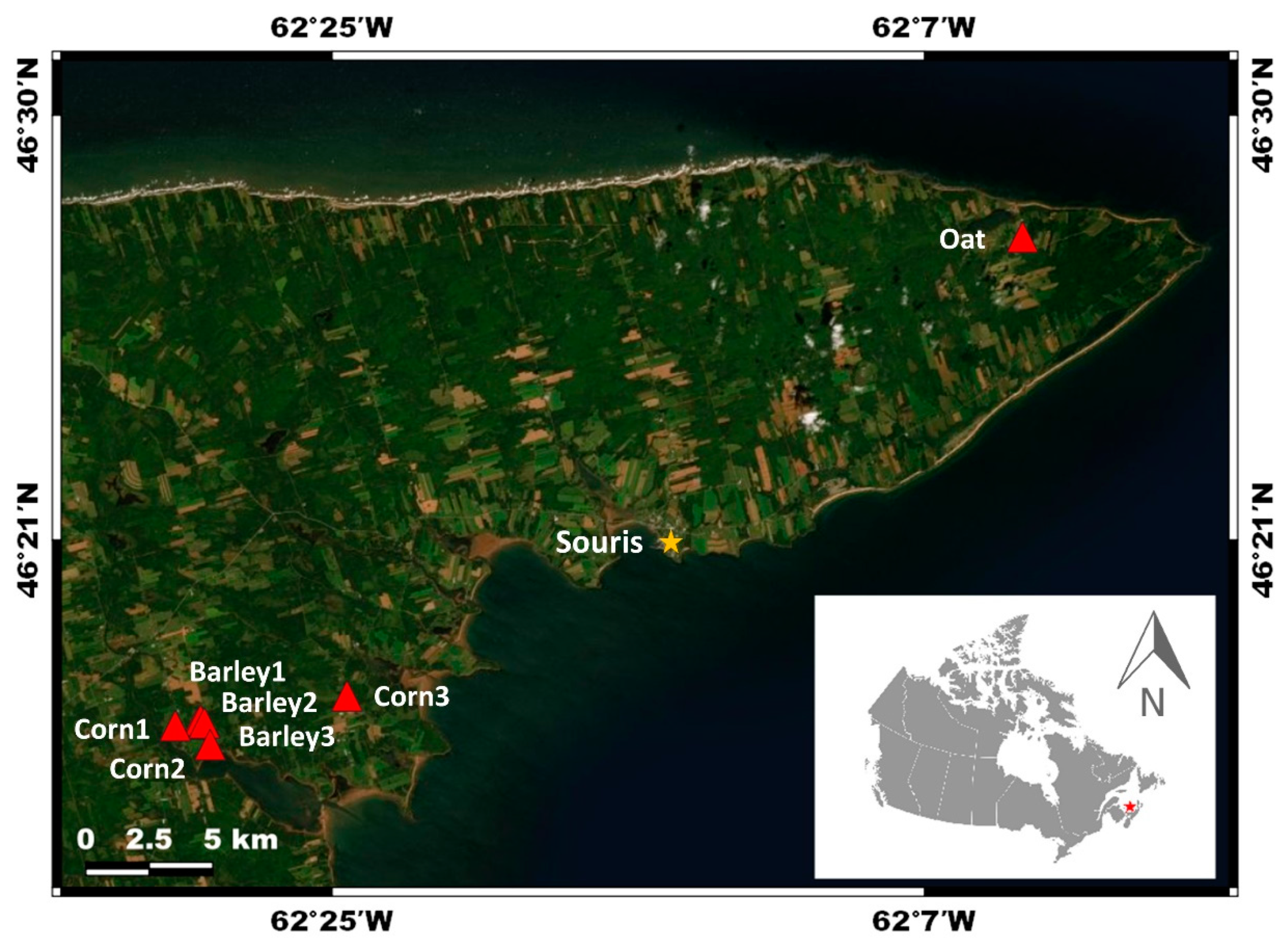
Figure 1.
Location of the study sites in Prince Edward Island. ESRI Satellite (ArcGIS/World Imagery).
Figure 1.
Location of the study sites in Prince Edward Island. ESRI Satellite (ArcGIS/World Imagery).
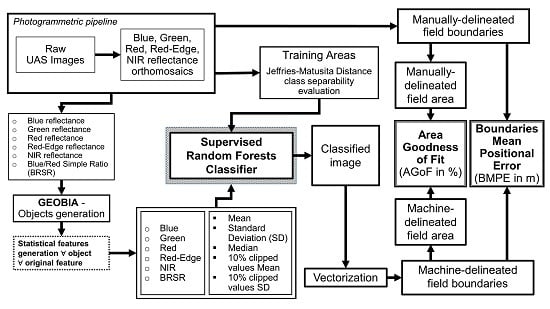
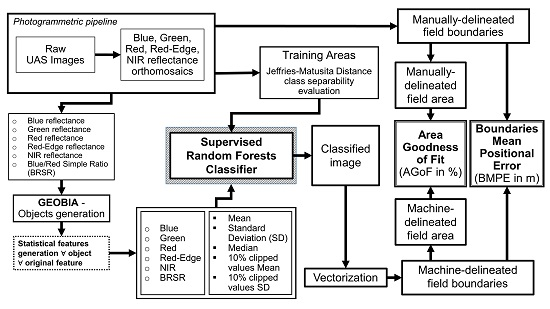
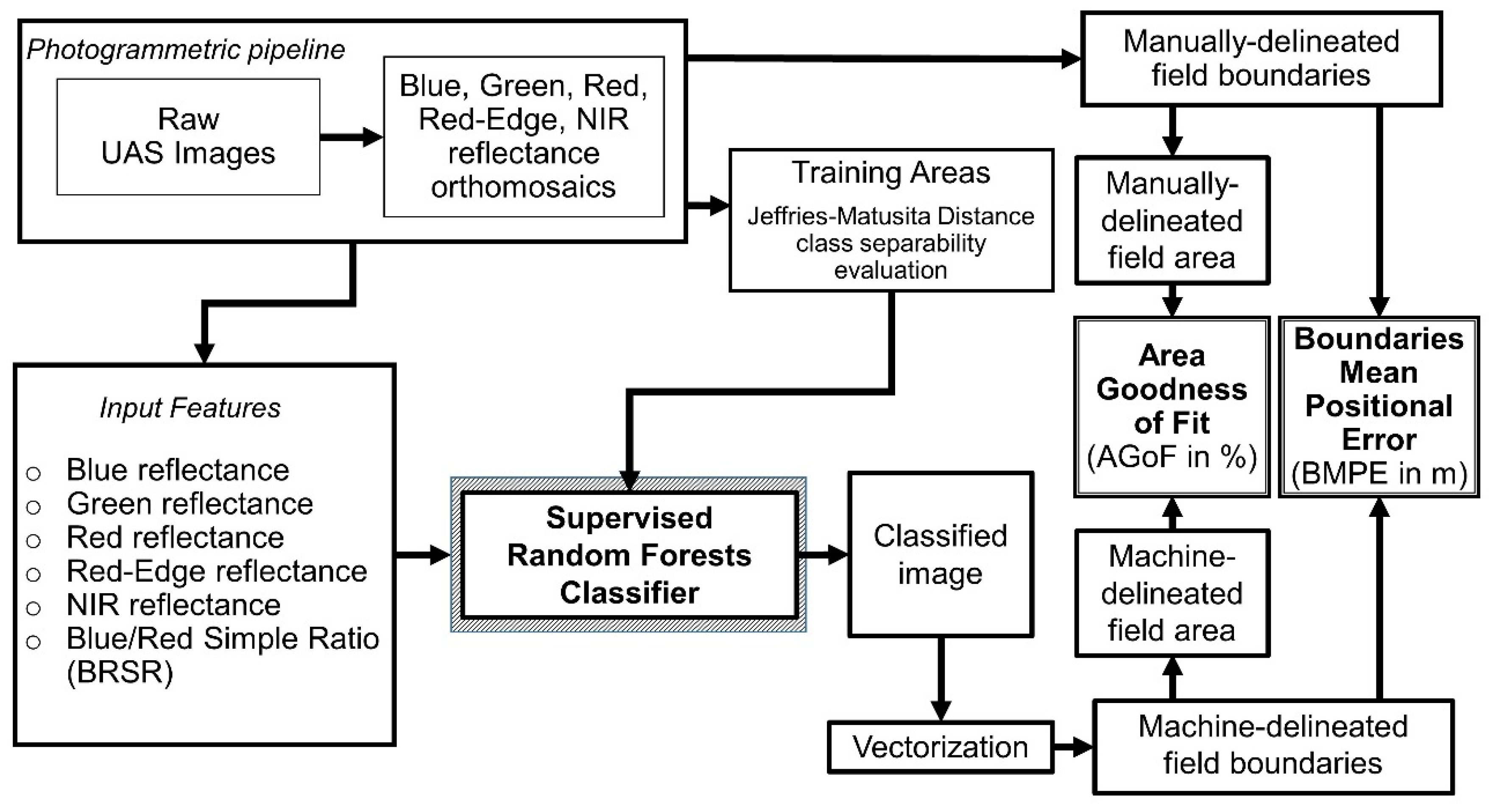
Figure 2.
Flowchart of the pixel-based image analysis (PBIA) methodology.
Figure 2.
Flowchart of the pixel-based image analysis (PBIA) methodology.
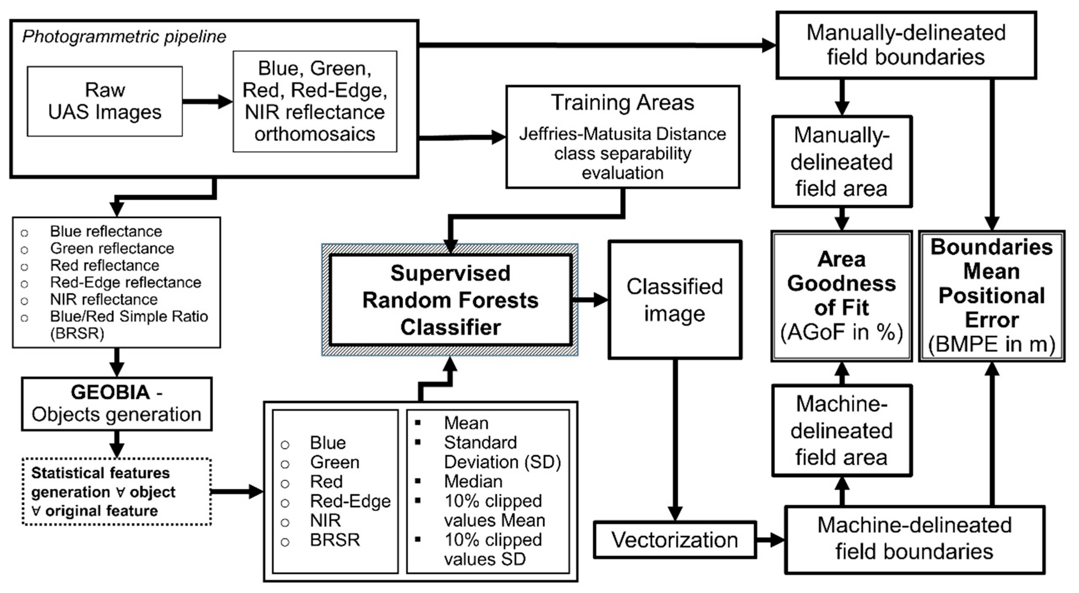
Figure 3.
Flowchart of the Geographic Object-Based Image Analysis (GEOBIA) methodology.
Figure 3.
Flowchart of the Geographic Object-Based Image Analysis (GEOBIA) methodology.
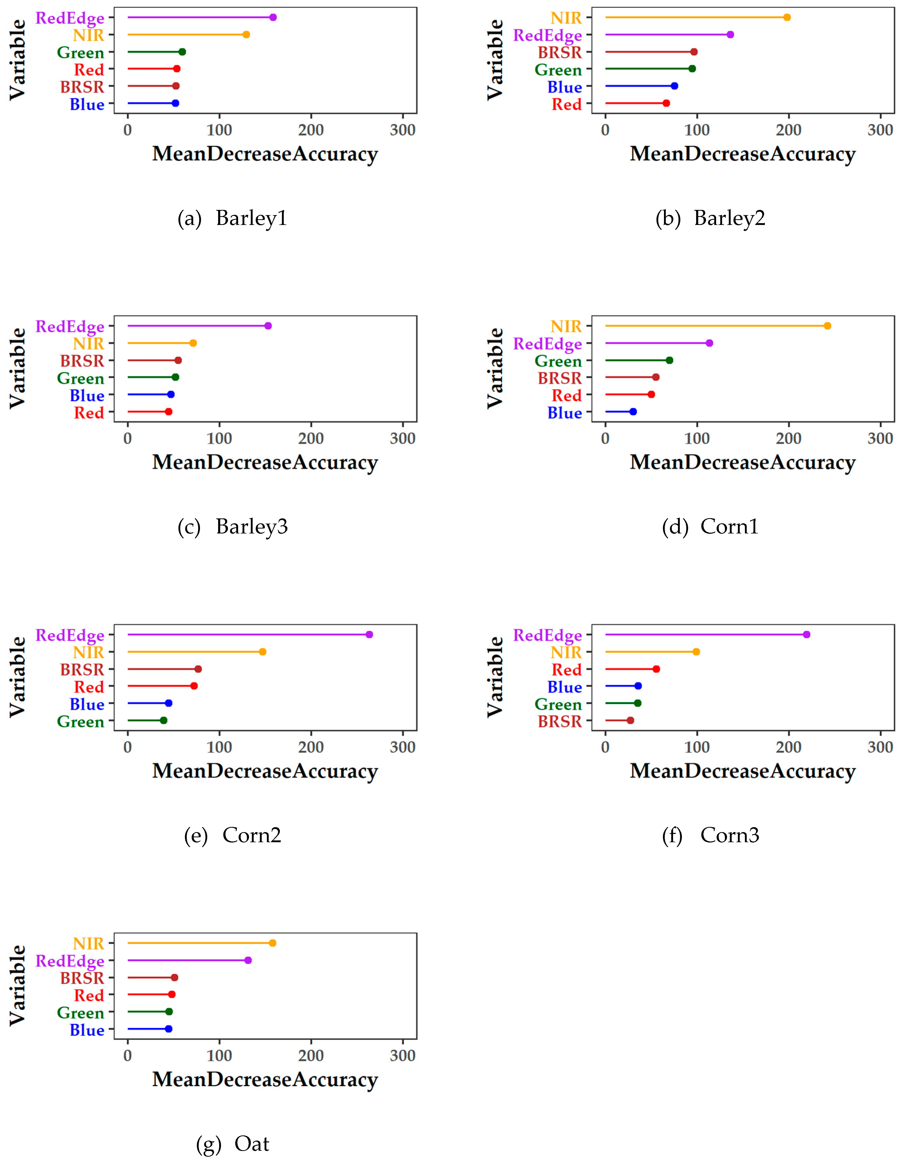
Figure 4.
Variable importance plot from the pixel-based image analysis random forest classifier for the following fields: (a) Barley1; (b) Barley2; (c) Barley3; (d) Corn1; (e) Corn2; (f) Corn3; (g) Oat.
Figure 4.
Variable importance plot from the pixel-based image analysis random forest classifier for the following fields: (a) Barley1; (b) Barley2; (c) Barley3; (d) Corn1; (e) Corn2; (f) Corn3; (g) Oat.
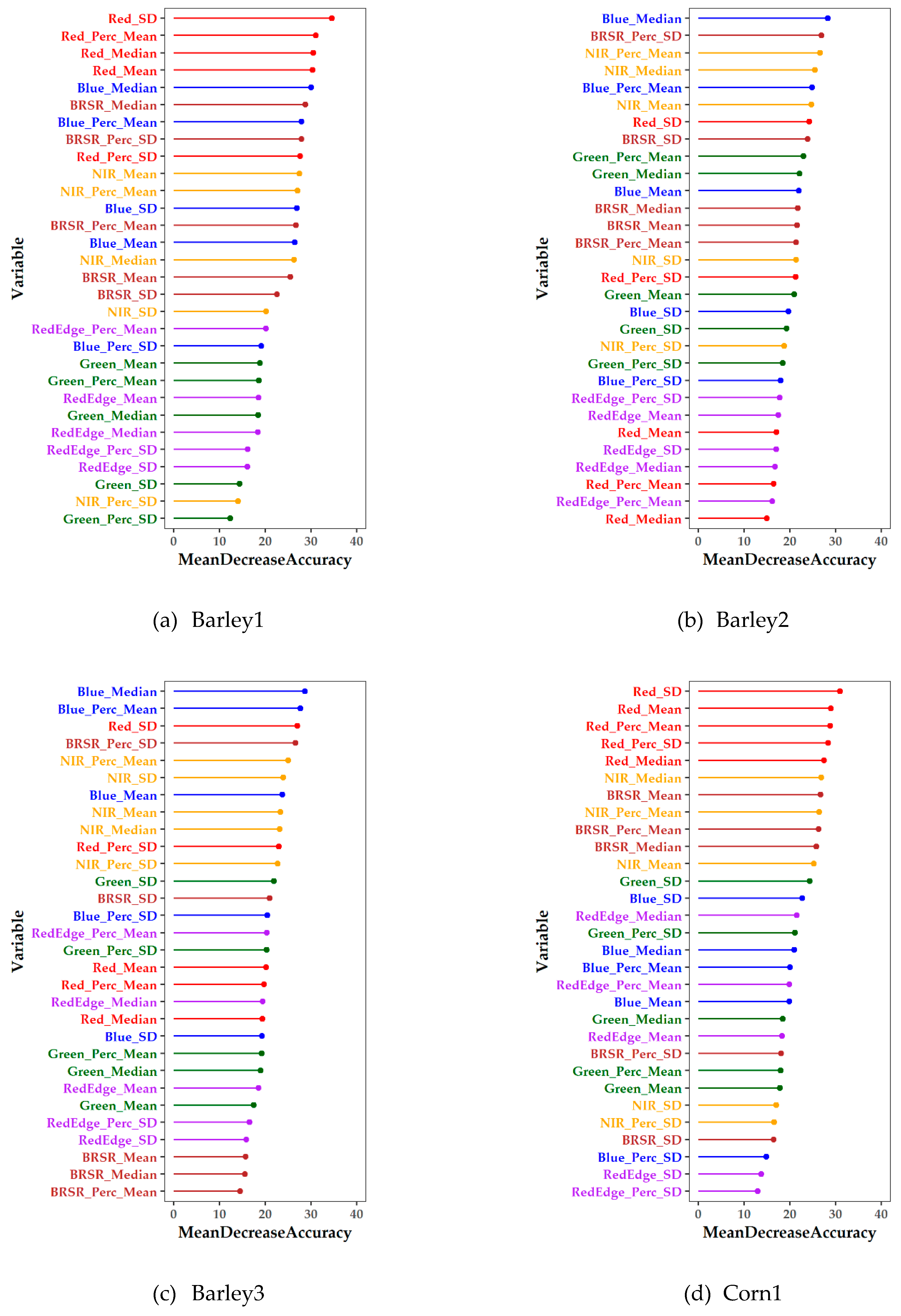
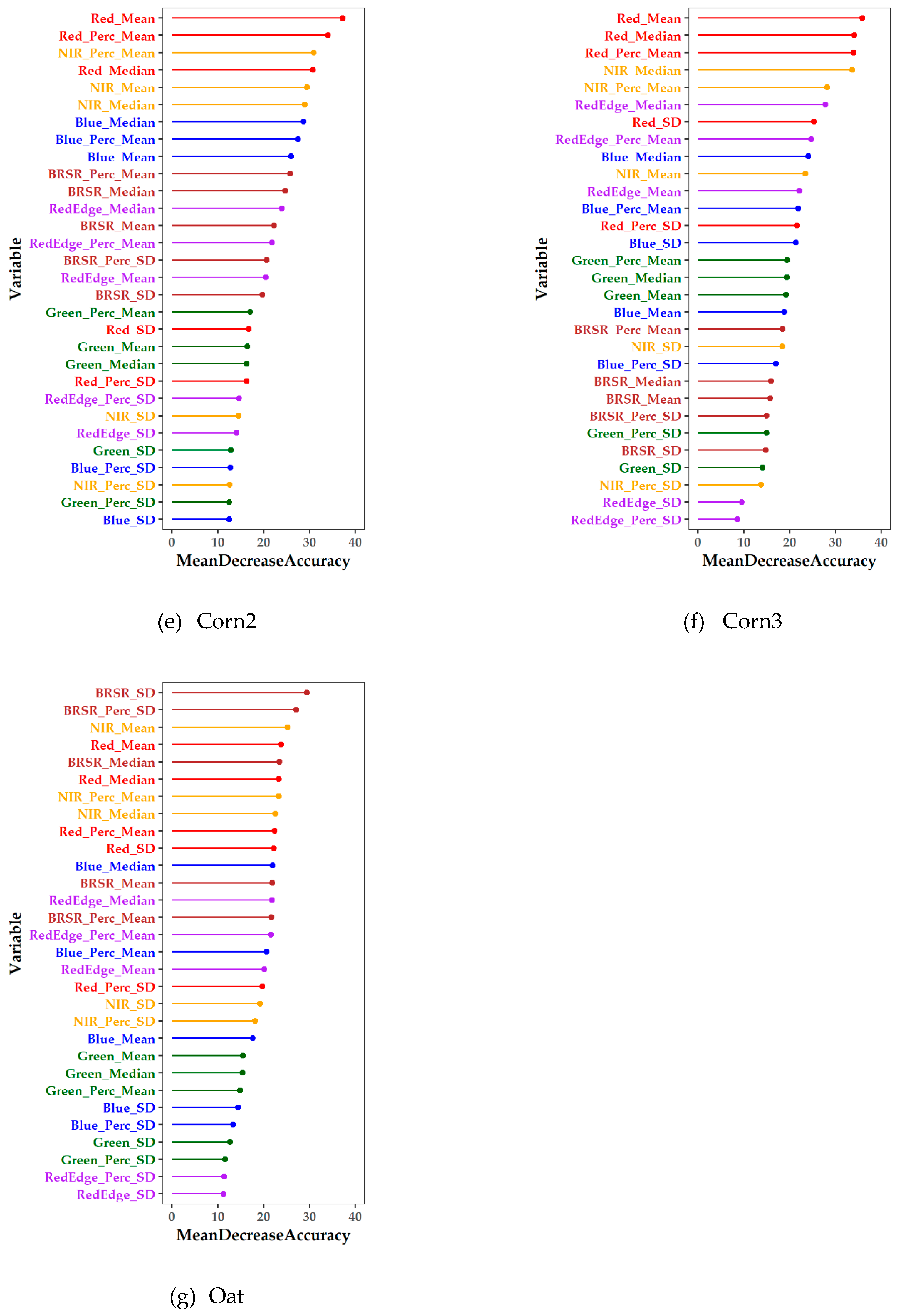
Figure 5.
Variable importance plot from the geographic object-based image analysis random forest classification for the following fields: (a) Barley1; (b) Barley2; (c) Barley3; (d) Corn1; (e) Corn2; (f) Corn3; (g) Oat.
Figure 5.
Variable importance plot from the geographic object-based image analysis random forest classification for the following fields: (a) Barley1; (b) Barley2; (c) Barley3; (d) Corn1; (e) Corn2; (f) Corn3; (g) Oat.
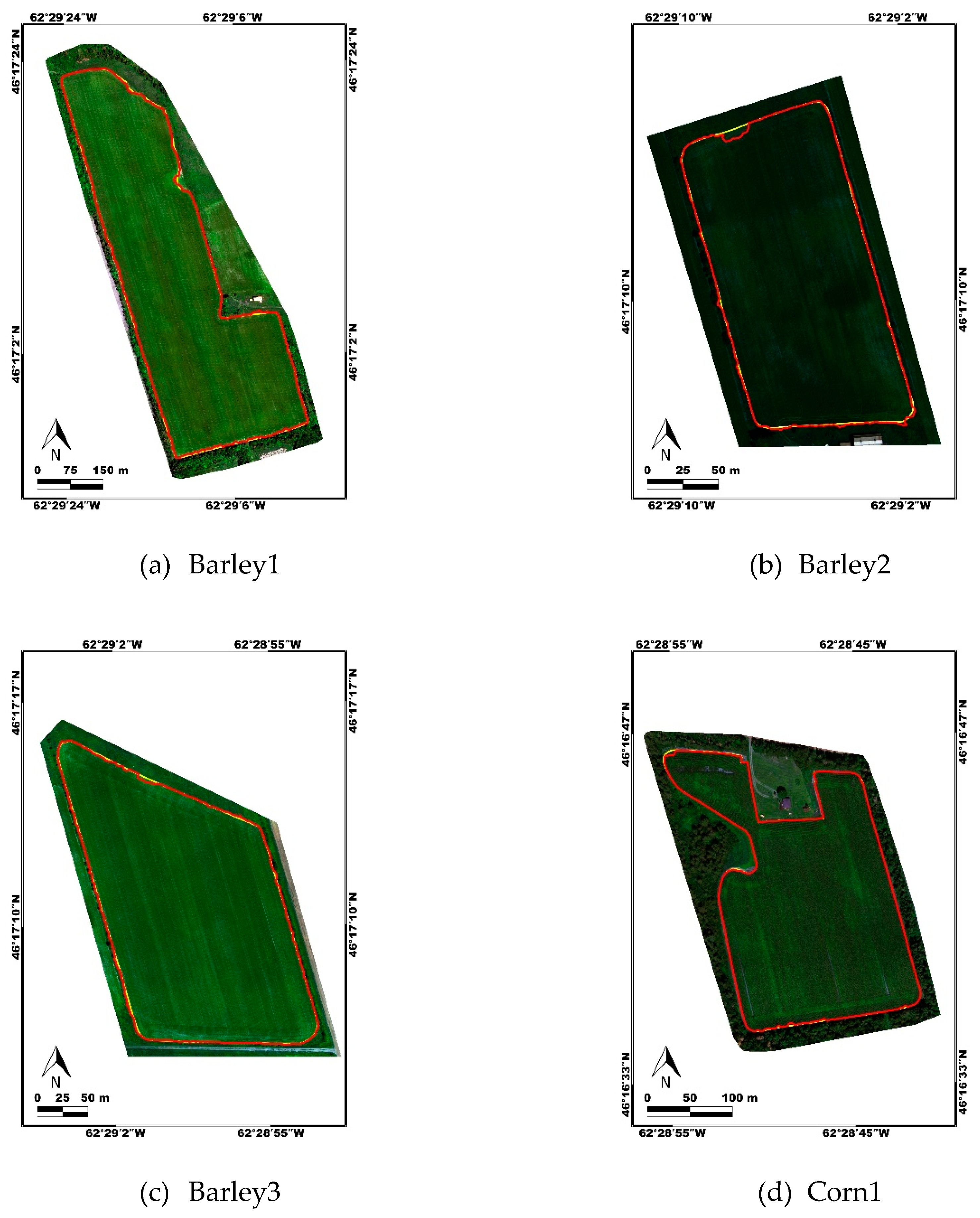
Figure 6.
Red, green and blue (RGB) image composites comparing the manually-delineated and PBIA-delineated borders for the following fields: (a) Barley1, (b) Barley2, (c) Barley3, (d) Corn1, (e) Corn2, (f) Corn3, (g) Oat; (h) Legend. The manually delineated borders are represented in yellow. The machine delineated borders are represented in red.
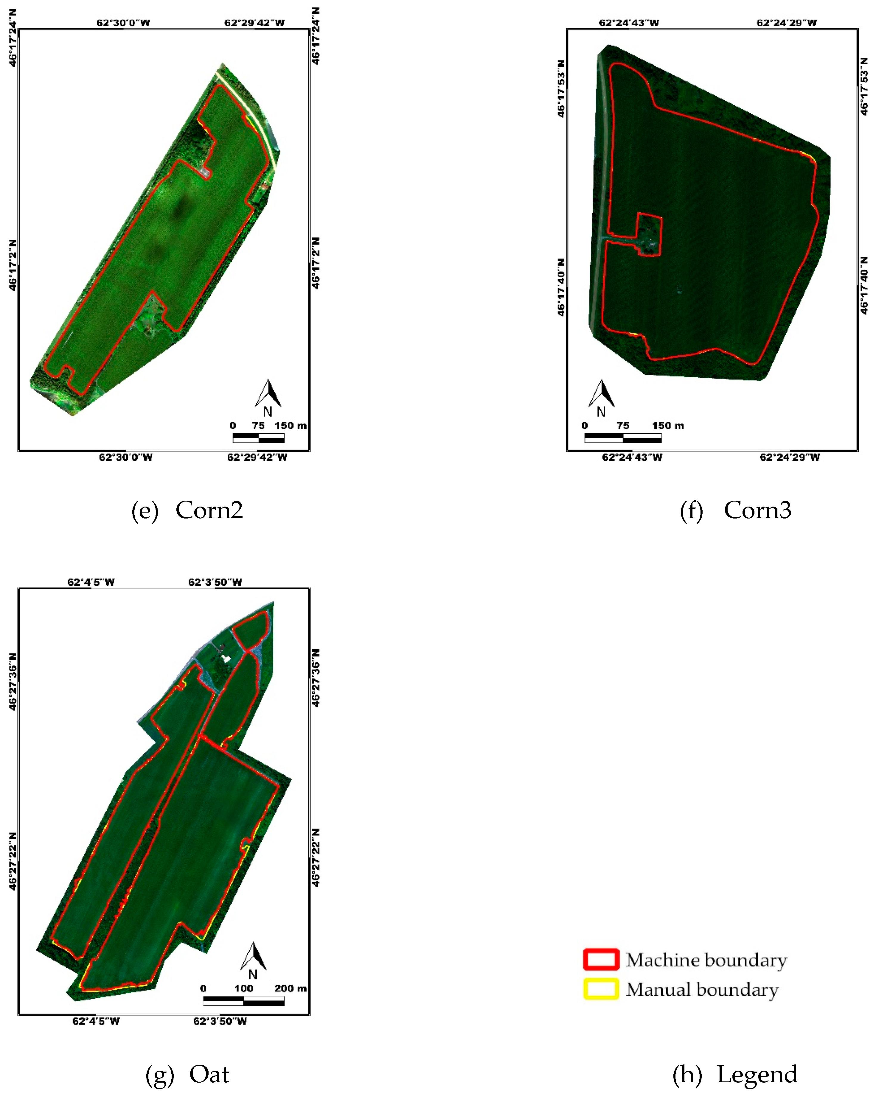
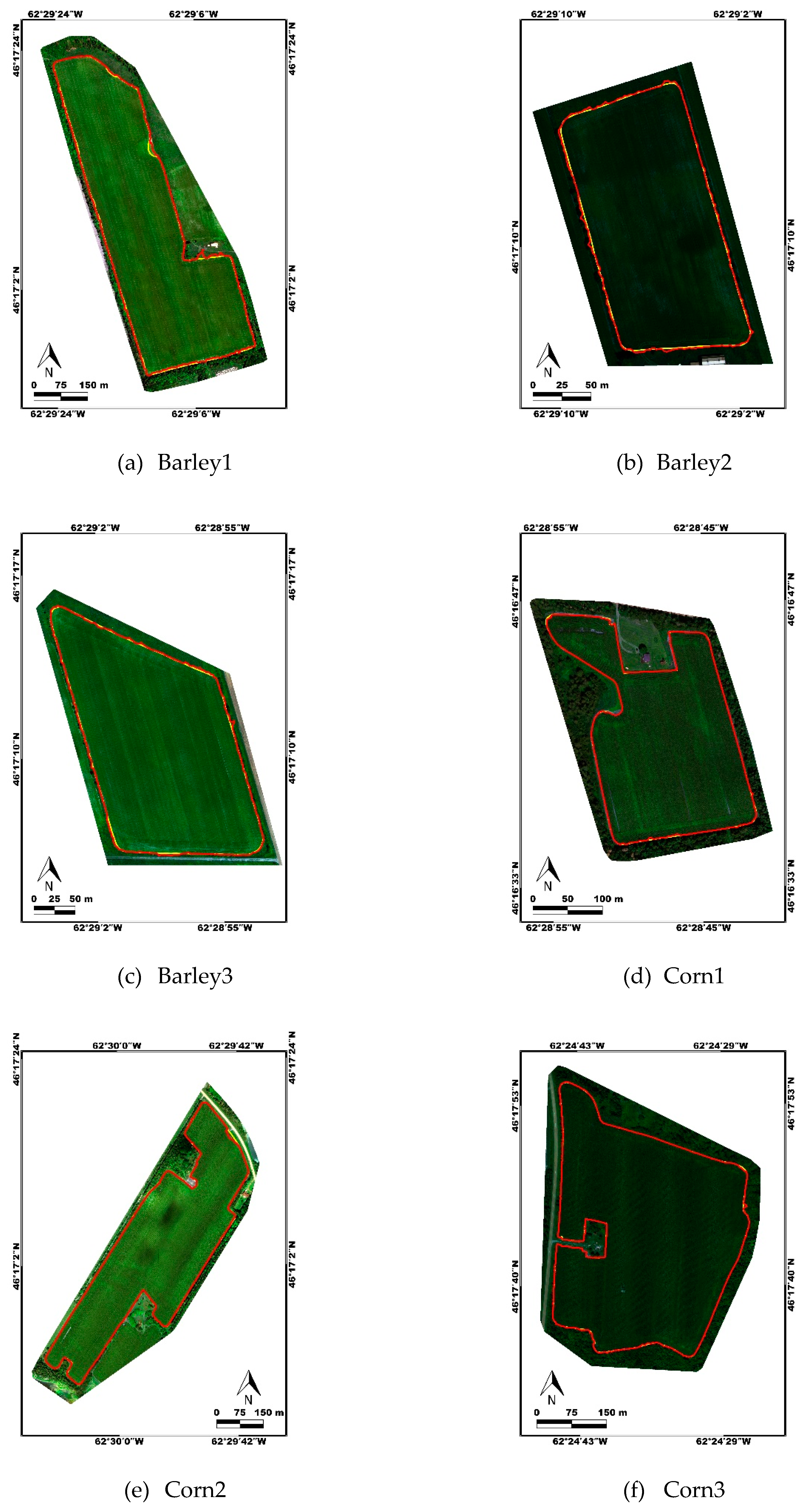
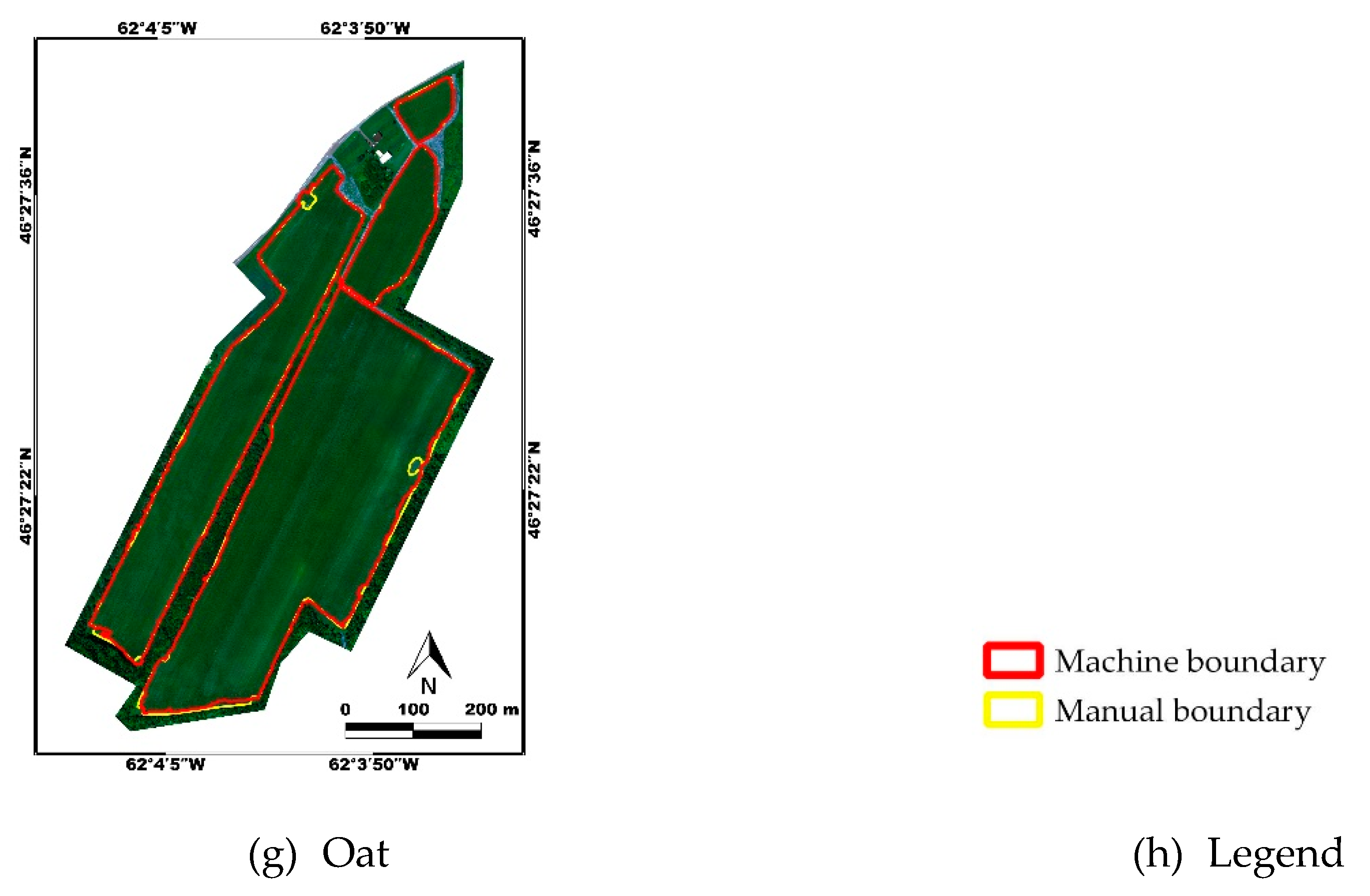
Figure 7.
RGB image composites comparing the manually-delineated and GEOBIA-delineated borders for the following fields: (a) Barley1, (b) Barley2, (c) Barley3, (d) Corn1, (e) Corn2, (f) Corn3, (g) Oat; (h) Legend. The manually delineated borders are represented in yellow. The machine delineated borders are represented in red.
Table 1.
Unmanned aircraft system (UAS) flight parameters.
Table 1.
Unmanned aircraft system (UAS) flight parameters.
| Flight Number | Field | Number of Images | Date | Time (UTC-3) | Area (m2) |
|---|
| F.1 | Barley1 | 3615 | 2018-07-20 | 11:30 | 310,131 |
| Barley2 | 34,832.00 |
| Barley3 | 61,282.00 |
| F.2 | Corn1 | 1345 | 2018-08-21 | 12:30 | 89,463.00 |
| F.3 | Corn2 | 2415 | 2018-08-21 | 13:00 | 309,163 |
| F.4 | Corn3 | 2450 | 2018-08-21 | 13:30 | 234,493 |
| F.5 | Oat | 2675 | 2018-07-20 | 14:00 | 301,261.40 |
Table 2.
MicaSense RedEdge band characteristics.
Table 2.
MicaSense RedEdge band characteristics.
| Band | Blue | Green | Red | Red-Edge | NIR |
|---|
| Range (nm) | 465–485 | 550–570 | 663–673 | 712–722 | 820–860 |
| Bandwidth (nm) | 20 | 20 | 10 | 10 | 40 |
| Central wavelength (nm) | 475 | 560 | 668 | 717 | 840 |
Table 3.
Number of training areas per class for PBIA.
Table 3.
Number of training areas per class for PBIA.
| Figure 1. | Soil | Crop | Other Vegetation | Total |
|---|
| Areas | Pixels | Areas | Pixels | Areas | Pixels | Areas | Pixels |
|---|
| Barley1 | 16 | 10,006 | 25 | 10,013 | 26 | 10,013 | 67 | 30,032 |
| Barley2 | 11 | 10,002 | 15 | 10,008 | 15 | 10,008 | 41 | 30,018 |
| Barley3 | 15 | 10,003 | 15 | 10,008 | 21 | 10,011 | 51 | 30,022 |
| Corn1 | 23 | 10,004 | 16 | 10,009 | 20 | 10,009 | 59 | 30,022 |
| Corn2 | 23 | 10,011 | 28 | 10,014 | 17 | 10,007 | 68 | 30,032 |
| Corn3 | 13 | 10,008 | 23 | 10,008 | 21 | 10,006 | 57 | 30,022 |
| Oat | 22 | 10,010 | 20 | 10,010 | 21 | 10,014 | 63 | 30,034 |
Table 4.
Number of objects and objects mean area (m2) per field.
Table 4.
Number of objects and objects mean area (m2) per field.
| Field | Number of Objects | Mean Object Area |
|---|
| Barley1 | 55,625 | 5.6 |
| Barley2 | 8944 | 3.9 |
| Barley3 | 11,153 | 5.5 |
| Corn1 | 23,118 | 3.9 |
| Corn2 | 44,057 | 7.0 |
| Corn3 | 58,897 | 3.9 |
| Oat | 38,558 | 7.8 |
Table 5.
List of the GEOBIA object features with their associated names used in the study.
Table 5.
List of the GEOBIA object features with their associated names used in the study.
| | Mean | Standard Deviation (SD) | Median | Mean - Percentiles | SD - Percentiles |
|---|
| Blue reflectance | Blue_Mean | Blue_SD | Blue_Median | Blue_Perc_Mean | Blue_ Perc_SD |
| Green reflectance | Green_Mean | Green_SD | Green_Median | Green_ Perc_Mean | Green_ Perc_SD |
| Red reflectance | Red_Mean | Red_SD | Red_Median | Red_ Perc_Mean | Red_ Perc_SD |
| Red-Edge reflectance | RedEdge_Mean | RedEdge_SD | RedEdge_Median | RedEdge_ Perc_Mean | RedEdge_ Perc_SD |
| NIR reflectance | NIR_Mean | NIR_SD | NIR_Median | NIR_ Perc_Mean | NIR_ Perc_SD |
| BRSR VI | BRSR_Mean | BRSR_SD | BRSR_Median | BRSR_ Perc_Mean | BRSR_ Perc_SD |
Table 6.
Number of training objects per class for GEOBIA and their mean object area (m2).
Table 6.
Number of training objects per class for GEOBIA and their mean object area (m2).
| Field | Soil | Crop | Other Vegetation | Total | Mean Object Area |
|---|
| Barley1 | 262 | 4526 | 5241 | 10,029 | 2.8 |
| Barley2 | 27 | 1502 | 542 | 2071 | 1.8 |
| Barley3 | 128 | 1610 | 716 | 2454 | 2.4 |
| Corn1 | 86 | 2419 | 1808 | 4313 | 1.9 |
| Corn2 | 321 | 4172 | 2049 | 6542 | 3.6 |
| Corn3 | 247 | 6387 | 3917 | 10,551 | 2.2 |
| Oat | 194 | 1930 | 3192 | 5316 | 3.6 |
Table 7.
Jeffries–Matusita distance between the three classes computed with the pixel-based image analysis training areas using the blue, green, red, red-edge, NIR reflectance, and BRSR VI features.
Table 7.
Jeffries–Matusita distance between the three classes computed with the pixel-based image analysis training areas using the blue, green, red, red-edge, NIR reflectance, and BRSR VI features.
| Field | Crop-Soil | Crop-Vegetation | Soil-Vegetation |
|---|
| Barley1 | 1.999925 | 1.782663 | 1.99192 |
| Barley2 | 1.973503 | 1.602653 | 1.962501 |
| Barley3 | 1.999999 | 1.322589 | 1.999988 |
| Corn1 | 1.999999 | 1.878568 | 1.999456 |
| Corn2 | 1.999999 | 1.929277 | 1.989666 |
| Corn3 | 1.999984 | 1.898402 | 1.998441 |
| Oat | 1.998787 | 1.846792 | 1.961582 |
| Average | 1.996028 | 1.751563 | 1.986222 |
Table 8.
Jeffries–Matusita distance between the three classes in the case of the geographic object-based image analysis classification using the full GEOBIA feature list of
Table 5.
Table 8.
Jeffries–Matusita distance between the three classes in the case of the geographic object-based image analysis classification using the full GEOBIA feature list of
Table 5.
| Field. | Crop-Soil | Crop-Vegetation | Soil-Vegetation |
|---|
| Barley1 | 1.999999 | 1.999672 | 1.999999 |
| Barley2 | 1.999854 | 1.960241 | 1.999805 |
| Barley3 | 1.999999 | 1.991511 | 1.999999 |
| Corn1 | 1.999999 | 1.999945 | 1.999999 |
| Corn2 | 1.999999 | 1.999992 | 1.999643 |
| Corn3 | 1.999999 | 1.999989 | 1.999996 |
| Oat | 1.999999 | 1.999997 | 1.999999 |
| Average | 1.999978 | 1.993049 | 1.999920 |
Table 9.
Random forest pixel-based image analysis and geographic object-based image analysis out-of-bag error rates (%) as a function of the field.
Table 9.
Random forest pixel-based image analysis and geographic object-based image analysis out-of-bag error rates (%) as a function of the field.
| Field | PBIA | GEOBIA |
|---|
| Barley1 | 2.96 | 2.17 |
| Barley2 | 7.17 | 6.23 |
| Barley3 | 5.11 | 4.97 |
| Corn1 | 1.38 | 1.32 |
| Corn2 | 1.33 | 1.02 |
| Corn3 | 0.89 | 0.65 |
| Oat | 1.77 | 1.20 |
| Average | 2.94 | 2.51 |
Table 10.
Confusion matrices and associated class user’s accuracies, producer’s accuracies, overall accuracies, errors of omission and errors of commission obtained by applying the PBIA random forest classifier to the blue, green, red, red-edge, near-infrared reflectance and blue-red simple ratio images. The bold diagonal number elements are the correctly classified pixels for each class.
| Field | Class | Soil | Crop | Other Vegetation | UA (%) | EC (%) | OA (%) |
|---|
| Barley1 | Soil | 9922 | 1 | 83 | 99.16 | 0.84 | 97.04 |
| | Crop | 13 | 9635 | 365 | 96.22 | 3.78 |
| | Other vegetation | 58 | 368 | 9587 | 95.75 | 4.25 |
| | PA (%) | 99.29 | 96.31 | 95.54 | | |
| | EO (%) | 0.71 | 3.69 | 4.46 | | |
| Barley2 | Soil | 9937 | 40 | 25 | 99.35 | 0.65 | 92.83 |
| | Crop | 154 | 9042 | 812 | 90.35 | 9.65 |
| | Other vegetation | 71 | 1051 | 8886 | 88.79 | 11.21 |
| | PA (%) | 97.79 | 89.23 | 91.39 | | |
| | EO (%) | 2.21 | 10.77 | 8.61 | | |
| Barley3 | Soil | 9998 | 4 | 1 | 99.95 | 0.05 | 94.89 |
| | Crop | 5 | 9517 | 486 | 95.09 | 4.91 |
| | Other vegetation | 6 | 1031 | 8974 | 89.64 | 10.36 |
| | PA (%) | 99.89 | 90.19 | 94.85 | | |
| | EO (%) | 0.11 | 9.81 | 5.15 | | |
| Corn1 | Soil | 9998 | 0 | 6 | 99.94 | 0.06 | 98.62 |
| | Crop | 0 | 9802 | 207 | 97.93 | 2.07 |
| | Other vegetation | 9 | 192 | 9808 | 97.99 | 2.01 |
| | PA (%) | 99.91 | 98.08 | 97.87 | | |
| | EO (%) | 0.09 | 1.92 | 2.13 | | |
| Corn2 | Soil | 9974 | 0 | 37 | 99.63 | 0.37 | 98.67 |
| | Crop | 4 | 9843 | 167 | 98.29 | 1.71 |
| | Other vegetation | 81 | 109 | 9817 | 98.10 | 1.90 |
| | PA (%) | 99.15 | 98.90 | 97.96 | | |
| | EO (%) | 0.85 | 1.10 | 2.04 | | |
| Corn3 | Soil | 9982 | 1 | 25 | 99.74 | 0.26 | 99.11 |
| | Crop | 0 | 9884 | 124 | 98.76 | 1.24 |
| | Other vegetation | 36 | 82 | 9888 | 98.82 | 1.18 |
| | PA (%) | 99.64 | 99.17 | 98.52 | | |
| | EO (%) | 0.36 | 0.83 | 1.48 | | |
| Oat | Soil | 9974 | 1 | 35 | 99.64 | 0.36 | 98.23 |
| | Crop | 8 | 9786 | 216 | 97.76 | 2.24 |
| | Other vegetation | 36 | 235 | 9743 | 97.29 | 2.71 |
| | PA (%) | 99.56 | 97.65 | 97.49 | | |
| | EO (%) | 0.44 | 2.35 | 2.51 | | |
Table 11.
Confusion matrices and associated class user’s accuracies, producer’s accuracies, overall accuracies, errors of omission and errors of commission obtained by applying the GEOBIA random forest classifier to the blue, green, red, red-edge, near-infrared reflectance and blue-red simple ratio images. The bold diagonal number elements are the correctly classified objects for each class.
| Field | Class | Soil | Crop | Other Vegetation | UA (%) | EC (%) | OA (%) |
|---|
| Barley1 | Soil | 252 | 2 | 8 | 96.18 | 3.82 | 97.83 |
| | Crop | 3 | 4440 | 114 | 97.43 | 2.57 |
| | Other vegetation | 7 | 84 | 5119 | 98.25 | 1.75 |
| | PA (%) | 96.18 | 98.10 | 97.67 | | |
| | EO (%) | 3.82 | 1.90 | 2.33 | | |
| Barley2 | Soil | 23 | 10 | 8 | 56.10 | 43.90 | 93.77 |
| | Crop | 2 | 1412 | 27 | 97.99 | 2.01 |
| | Other vegetation | 2 | 80 | 507 | 86.08 | 13.92 |
| | PA (%) | 85.19 | 94.01 | 93.54 | | |
| | EO (%) | 14.81 | 5.99 | 6.46 | | |
| Barley3 | Soil | 126 | 2 | 1 | 97.67 | 2.33 | 95.03 |
| | Crop | 2 | 1524 | 33 | 97.75 | 2.25 |
| | Other vegetation | 0 | 84 | 682 | 89.03 | 10.97 |
| | PA (%) | 98.44 | 94.66 | 95.25 | | |
| | EO (%) | 1.56 | 5.34 | 4.75 | | |
| Corn1 | Soil | 86 | 0 | 5 | 94.51 | 5.49 | 98.68 |
| | Crop | 0 | 2400 | 33 | 98.64 | 1.36 |
| | Other vegetation | 0 | 19 | 1770 | 98.94 | 1.06 |
| | PA (%) | 100.00 | 99.21 | 97.90 | | |
| | EO (%) | 0.00 | 0.79 | 2.10 | | |
| Corn2 | Soil | 310 | 0 | 13 | 95.98 | 4.02 | 98.98 |
| | Crop | 1 | 4157 | 28 | 99.31 | 0.69 |
| | Other vegetation | 10 | 15 | 2008 | 98.77 | 1.23 |
| | PA (%) | 96.57 | 99.64 | 98.00 | | |
| | EO (%) | 3.43 | 0.36 | 2.00 | | |
| Corn3 | Soil | 241 | 3 | 13 | 93.77 | 6.23 | 99.36 |
| | Crop | 0 | 6366 | 28 | 99.56 | 0.44 |
| | Other vegetation | 6 | 18 | 3876 | 99.38 | 0.62 |
| | PA (%) | 97.57 | 99.67 | 98.95 | | |
| | EO (%) | 2.43 | 0.33 | 1.05 | | |
| Oat | Soil | 188 | 0 | 7 | 96.41 | 3.59 | 98.80 |
| | Crop | 2 | 1919 | 40 | 97.86 | 2.14 |
| | Other vegetation | 4 | 11 | 3145 | 99.53 | 0.47 |
| | PA (%) | 96.91 | 99.43 | 98.53 | | |
| | EO (%) | 3.09 | 0.57 | 1.47 | | |
Table 12.
Area goodness of fit (%) computed by comparing the manually- and machine-delineated field areas for the pixel-based image analysis and geographic object-based image analysis classifications.
Table 12.
Area goodness of fit (%) computed by comparing the manually- and machine-delineated field areas for the pixel-based image analysis and geographic object-based image analysis classifications.
| Field | PBIA | GEOBIA | (PBIA-GEOBIA) |
|---|
| Barley1 | 98.91 | 98.40 | 0.51 |
| Barley2 | 98.89 | 98.32 | 0.57 |
| Barley3 | 99.03 | 98.96 | 0.07 |
| Corn1 | 99.10 | 99.03 | 0.07 |
| Corn2 | 99.26 | 99.47 | –0.21 |
| Corn3 | 99.74 | 99.68 | 0.06 |
| Oat | 97.48 | 97.62 | –0.14 |
| Average | 98.91 | 98.78 | 0.13 |
Table 13.
Boundary mean positional error (in meters) computed by comparing the manually- and machine-delineated field boundaries for the pixel-based image analysis and geographic object-based image analysis classifications.
Table 13.
Boundary mean positional error (in meters) computed by comparing the manually- and machine-delineated field boundaries for the pixel-based image analysis and geographic object-based image analysis classifications.
| Field | PBIA | GEOBIA | (PBIA-GEOBIA) |
|---|
| Barley1 | 1.05 | 1.72 | −0.67 |
| Barley2 | 0.62 | 0.69 | −0.07 |
| Barley3 | 0.58 | 0.63 | −0.05 |
| Corn1 | 0.26 | 0.24 | 0.02 |
| Corn2 | 0.61 | 0.44 | 0.17 |
| Corn3 | 0.32 | 0.37 | −0.05 |
| Oat | 1.34 | 1.21 | 0.13 |
| Average | 0.68 | 0.76 | −0.08 |

 ,
, 


