Article

Dynamics and Drivers of the Alpine Timberline on Gongga Mountain of Tibetan Plateau-Adopted from the Otsu Method on Google Earth Engine

1
School of Civil Engineering and Geomatics, Southwest Petroleum University, Chengdu 610500, China
2
Synthesis Research Centre of Chinese Ecosystem Research Network, Key Laboratory of Ecosystem Network Observation and Modelling, Institute of Geographic Sciences and Natural Resources Research, Chinese Academy of Sciences, Beijing 100101, China
3
Chengdu Institute of Biology, Chinese Academy of Sciences, Chengdu 610041, China
*
Author to whom correspondence should be addressed.
Remote Sens. 2020, 12(16), 2651; https://0-doi-org.brum.beds.ac.uk/10.3390/rs12162651
Submission received: 17 July 2020 / Revised: 3 August 2020 / Accepted: 14 August 2020 / Published: 17 August 2020

Abstract

:
The alpine timberline, an ecosystem ecotone, indicates climatic change and is tending to shift toward higher altitudes because of an increase in global warming. However, spatiotemporal variations of the alpine timberline are not consistent on a global scale. The abundant and highest alpine timberline, located on the Tibetan Plateau, is less subject to human activity and disturbance. Although many studies have investigated the alpine timberline on the Tibetan Plateau, large-scale monitoring of spatial-temporal dynamics and driving mechanisms of the alpine timberline remain uncertain and inaccurate. Hence, the Gongga Mountain on the southeastern Tibetan Plateau was chosen as the study area because of the most complete natural altitudinal zonation. We used the Otsu method on Google Earth Engine to extract the alpine timberline from 1987–2019 based on the normalized difference vegetation index (NDVI). Then, the alpine timberline spatiotemporal patterns and the effect of topography on alpine timberline distribution were explored. Four hillsides on the western Gongga Mountain were selected to examine the hillside differences and drivers of the alpine timberline based on principal component analysis (PCA) and multiple linear regression (MLR). The results indicated that the elevation range of alpine timberline was 3203–4889 m, and the vegetation coverage increased significantly (p < 0.01) near the alpine timberline ecotone on Gongga Mountain. Moreover, there was spatial heterogeneity in dynamics of alpine timberline, and some regions showed no regular trend in variations. The spatial pattern of the alpine timberline was generally high in the west, low in the east, and primarily distributed on 15–55° slopes. Besides, the drivers of the alpine timberline have the hillside differences, and the sunny and shady slopes possessed different driving factors. Thus, our results highlight the effects of topography and climate on the alpine timberline on different hillsides. These findings could provide a better approach to study the dynamics and formation of alpine timberlines.

Graphical Abstract

1. Introduction

Structure, ecosystem processes, and functions of global vegetation communities and human livelihood have been seriously impacted adversely by climate change over the past 100 years [1]. Terrestrial ecosystems are undergoing long lasting, complex, and unpredictable changes as a consequence of variations in the global climate [2,3]. Vegetation, as a natural bond between soil, air and water, is crucial for global biodiversity conservation, ecosystem services and vision of human beings, however, it is highly sensitive to climate change [4]. Over the past few decades, terrestrial vegetation activity and growing season time in the Northern Hemisphere have increased with increase in temperatures [5,6,7]. Several cases worldwide have indicated that diverse vegetation patterns are greatly altered by global warming. For instance, the Arctic tundra has been encroached upon by shrubs, affecting ecosystem function, carbon storage, wildlife habitats, and hydrological status and processes [8,9]. Particularly, in the ecosystem ecotone (such as alpine timberlines), the vegetation community structure, function and spatial pattern are especially sensitive to global change [10,11].
The “alpine timberline” is a transition zone alternating between trees, shrubs, and grasslands along altitude gradients [12,13]. Environments in alpine timberline ecotone are characterized by lower annual temperatures and insufficient precipitation, resulting in which the trees experience cold climate and physiological drought that hamper their growth [14]. Additionally, the alpine timberline fluctuates with variations in multiple factors, such as dominant tree species, topography, and climatic conditions [15]. Alpine timberline dynamics in different regions currently present distinct characteristics. For example, based on nearly 70 years of historical maps and modern satellite imagery in the Ukrainian Carpathians, researchers found that the altitude of timberline had risen by 1.14 m year−1, and the area covered by one-third of the pastures had increased [16]. In the alpine region of the Himalayas, the timberline shifted 10 m year−1 from the 1970s to 2006 [17]. Near the Yamunotri watershed, the alpine timberline moved to a higher altitude at an average rate of 4 m year−1 during the past 20 years [18]. However, the response trend of alpine timberline displacement to climate warming remains poorly understood, especially in the brittle ecosystem of the Tibetan Plateau.
The alpine timberline—critical for maintaining alpine biodiversity and functioning montane ecosystems—is the long-term result of natural environmental conditions and is extremely sensitive to global change [3,19]. The gradual decrease in temperature with elevation in montane systems greatly influences vegetation metabolic processes and alpine timberline formation [3,20]. Therefore, temperature is generally regarded as the primary driver of alpine timberline [21]. On a global scale, the alpine timberline possessed a trend consistent with the global ground isotherm (6.7 ± 0.8 °C) [22]. However, changing temperatures in different regions create an asynchronism between the dynamics of alpine timberline and global warming [23,24]. Studies in the European Alps indicate that alpine timberlines are strongly correlated with temperatures in the hottest month [13]. In northern Russia, summer temperatures and the vegetation growing season largely determine the location of the alpine timberline [25]. In China, the temperature during the growing season is the primary climatic factor affecting the altitude of the alpine timberline [26]. Additionally, rainfall is also an important factor regulating alpine timberlines in some regions and can improve growth conditions [27,28]. In short, water and heat conditions are the key drivers affecting alpine timberlines; however, the dynamic mechanisms involved remain undetermined as yet.
Gongga Mountain, located at the south-eastern edge of the Tibetan Plateau, belongs to the transition zone between the Sichuan Basin and the Tibetan Plateau. Because of the intact altitudinal zonation, Gongga Mountain is an ideal place to address the spatiotemporal dynamic and formation mechanism of the alpine timberline [29,30]. Previous studies obtained alpine timberline information mainly from historical data and field investigation [31,32]. Although field survey has benign accuracy and reliability, the relatively smaller scale restricts operational efficiency and broad applicability. Additionally, field surveys are inconvenient for monitoring long-term dynamic changes of alpine timberline on a large scale. Thus, exploring a new method to resolve dynamic tendency, spatial patterns, and drivers of alpine timberline is essential.
Remote sensing and geographic information technologies have recently become a practical means to identify the spatial distribution of alpine timberline [33,34]. The extraction methods of alpine timberline are mainly based on the supervised classification extraction and empirical normalized difference vegetation index (NDVI) values [35,36,37,38]. However, supervised classification requires the selection of training samples and human intervention, and these are characterized by several uncertainties with regard to the long-term monitoring of alpine timberlines. Meanwhile, the alpine timberline obtained by vegetation type boundaries is inaccurate, violating the timberline ecotone definition. Furthermore, empirical NDVI value is not very adaptable to different times, regions, and image data. The Otsu algorithm (the adaptive threshold algorithm) is introduced into Google Earth Engine to automatically determine the NDVI threshold of the alpine timberline ecotone, which addresses the aforementioned complications and improve computing efficiency. The Otsu algorithm finds an optimal threshold to distinguish relatively homogenous objects by maximising the inter-class variance [39,40,41]. Since the alpine timberline is an ecotone, the ecological vulnerability here is the lowest and the vegetation changes are the most unstable. Therefore, we retain vegetation and remove other land types (such as snow mountains, bare land, lakes and so on), and use the Otsu algorithm to obtain the NDVI threshold in the alpine timberline and to determine the location of the alpine timberline. The Google Earth Engine platform provides common remote sensing image data sets that can be called and calculated on online, providing convenience for the long-term monitoring of alpine timberlines [42,43].
Given these problems and new method, we calculated the NDVI based on Landsat imagery from 1987–2019, applied the Otsu method to Google Earth Engine, and obtained climate raster data by spatial interpolation that was based on terrain and generated topographic data by spatial analysis in the ArcGIS 10.2 software (ESRI, Inc., Redlands, CA, USA) across Gongga Mountain. Our primary objectives were: (1) determining the NDVI threshold of alpine timberline via the Otsu algorithm, (2) analysing spatial and temporal dynamics of the alpine timberline and exploring the effects of topography on alpine timberline distribution, and (3) revealing the comprehensive relationships among alpine timberline, topographic and climatic factors and discussing the variations of alpine timberline in future.

2. Materials and Methods
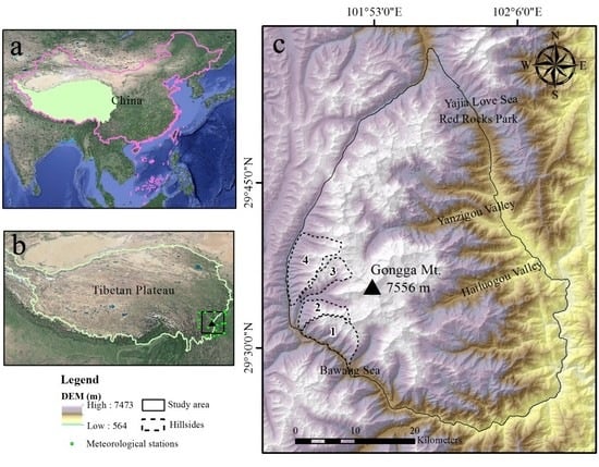
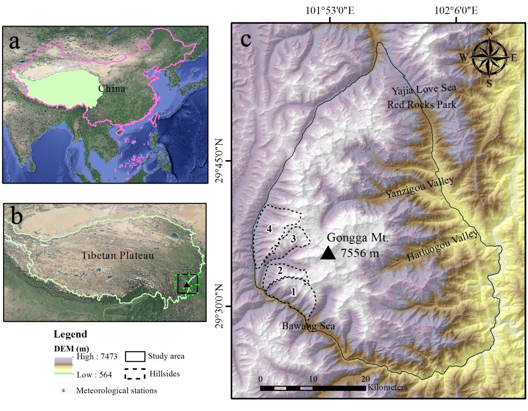
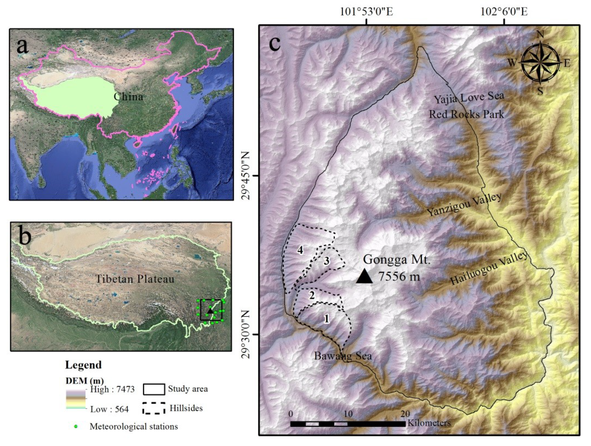
2.1. Study Area

The highest peak of Gongga Mountain (29°22′–29°57′N, 101°45′–102°10′E) is 7556 m above sea level (Figure 1).
Gongga Mountain features a geomorphic high mountain and deep valley landscape with average annual temperature and precipitation of 4.2 °C and 1947 mm, respectively [44,45], and possesses a transitional seasonal climate between the subtropical humid monsoon and the cold Tibetan Plateau climates, which is dominated by the southeast Pacific monsoon [30,32]. Because of the complex and varied natural geographical conditions, ecosystem types and biodiversity are extremely rich on Gongga Mountain. The integrity of natural altitudinal zonation ranging from subtropical to alpine vegetation is unique, making Gongga Mountain become an ideal area for studying alpine timberline in China [46]. In addition, Gongga Mountain is a national nature reserve surrounded by scenic spots. Of these, the Hailuogou is a national forest park, as the national 5A level scenic spot, which is the only glacier forest park in China and is a very popular tourist destination.

2.2. Data Sources and Platform

2.2.1. Landsat Satellite Imagery

The long-term monitoring of vegetation and land cover changes is supported by Landsat satellite imagery, which provides uninterrupted global multispectral surface imagery in 16-d intervals from July 1972 to the present [47]. We calculated the NDVI from 1987–2019 using satellite images with a 30 m spatial resolution from Landsat 5, 7, and 8. We discarded images from 2002, 2010, and 2017 because of severe cloud cover and missing image.

2.2.2. Meteorological Data

The annual and monthly meteorological data from 1987–2019 used in this study were collected from the China Meteorological Data Service Center (http://data.cma.cn). To improve the reliability and accuracy of climate data, we selected data from 17 meteorological stations in Kangting, Jiulong, Yuexi, Daofu, Xiaojin, Wenjiang, Dujiangyan, Xinlong, Litang, Daocheng, Hanyuan, Emeishan, Leshan, Muli, ZhaoJiao, Leibo, and Xichang. The average annual temperature (Year_TEM), precipitation (Year_PRE), growing season temperature (Grow_TEM), maximum growing season temperature (Grow_maxTEM), minimum growing season temperature (Grow_minTEM), and growing season precipitation (Grow_PRE)—with a 250-m resolution—were obtained by terrain interpolation with the Anusplin 4.2 software. The growing season ranged from May–September each year.

2.2.3. Topographic Data

The Digital Elevation Model (DEM) data are collected from the Advanced Spaceborne Thermal Emission and Reflection Radiometer Global Digital Elevation Model (ASTER GDEM) Version 3 (V3) provided by NASA EARTH DATA (https://earthdata.nasa.gov) [48]. The spatial resolution of the ASTER GDEM image is 30 m. The DEM vertical accuracy and horizontal resolution are 12.1 and 72 m, respectively. The DEM data are processed with ARCGIS10.2 software to obtain topographic factors (i.e., slope and aspect).

2.2.4. Google Earth Engine

Google Earth Engine (https://earthengine.google.com)—a platform with massive computational capabilities that can solve many geospatial analysis [42]. In this cloud-based platform, multiple researchers can simultaneously access open remote sensing product data and perform geospatial analysis on planet scale [43]. Common remote sensing products are efficiently processed through massive parallelisation using JavaScript or Python. We calculated the NDVI from Landsat satellite imagery and extracted the alpine timberline by the code editor on Google Earth Engine.

2.3. Methods

2.3.1. Otsu Method

In image interpretation, we usually want a method to automatically differentiate relatively homogenous categories such as land and water or forest and grass [49]. For single band images, two types classification can be implemented by finding an optimal Otsu threshold [39,40,41]. The Otsu method is an automatic and efficient way to realise cluster-based automatic image segmentation without depending on other priori information; furthermore, Otsu method possesses the flexible adaptation for different data and allows to monitor different ground targets including herbaceous crops, forest and surface water [50,51]. In this study, we used the Otsu method to identify the alpine timberline. Optimal thresholds are calculated by maximising the inter-class variance (ICV) of the pixel value distribution. The average grey degree and the inter-class variance are defined as follows [39]:
μ = n 0 n μ 0 + n 1 n μ 1 = ω 0 μ 0 + ω 1 μ 1
ICV = ω 0 ( μ 0 μ ) 2 + ω 1 ( μ 1 μ ) 2 = ω 0 ω 1 ( μ 0 μ 1 ) 2
where μ and ICV express the average grey degree and inter-class variance, respectively; n0 is the number of pixels less than the threshold; n1 is the number of pixels more than the threshold; n is the total number of pixels in the image; μ0 and μ1 are the average greyscale of the target and non-target categories, respectively; and ω0 and ω1 are the proportions of target and non-target pixels in the total pixels, respectively. The optimal threshold is obtained by traversing each grey value and comparing the inter-class variance.
We conducted Otsu analysis on vegetation using the NDVI, and the obtained threshold was used as a criterion for extracting the alpine timberline. In order to extract alpine timberline better, we calculated the NDVI for the early growing season with Landsat images. The NDVI is defined as:
NDVI = ( NIR Red ) ( NIR + Red )
where NIR and Red are the spectral reflectance values calculated in the near-infrared and red bands, respectively. We screened out regions with NDVI greater than 0.1 in Landsat images for the Otsu method analysis to reduce the impact of non-vegetated areas [52,53] and ultimately acquired the optimal Otsu threshold.

2.3.2. Alpine Timberline Extraction

We smoothed the NDVI images by convolving with a Gaussian kernel (which is generated from a continuous Gaussian signal on Google Earth Engine) to obtain NDVI threshold pixels and to detect dynamic alpine timberline changes. The contour line was obtained by the edge detection of NDVI pixels. We used a zero-crossing edge detection method, which identifies the zero-crossings value on each frequency band of the image. Next, we selected the contour line with a property value equal to the threshold value; pixels on the contour line are the alpine timberline points. The alpine timberline points were also post-processed (discussed later in Section 2.4).

2.3.3. Slope and Aspect Classification

Gongga Mountain has a marked vertical span of more than 6000 m. Slope, a significant geomorphological parameter, is the angle between the land surface and the horizontal plane expressed in degrees. Different slopes may affect the growth of trees, and higher slopes have more unstable foundations. The slope on Gongga Mountain is categorised as flat, very gentle, gentle, moderate, moderately steep, steep, and very steep for slope ranges of 0–2°, 2–5°, 5–15°, 15–25°, 25–35°, 35–55°, and more than 55°, respectively [54]. Table 1 presents the slope classification of Gongga Mountain.
The compass direction on a topographic slope is definition of aspect, usually starts at geographic north. Aspect strongly influences the radiation intensity, sunshine hours, and temperature, water, and soil conditions of different slopes, affecting vegetation growth and the distribution characteristics of the alpine timberline. Flat ground has no slope or aspect. The aspects of Gongga Mountain are classified as flat (−1), north (0–22.5° and 227.5–360°), northeast (22.5–67.5°), east (67.5–112.5°), southeast (112.5–157.5°), south (157.5–202.5°), southwest (202.5–247.5°), west (247.5–292.5°), and northwest (292.5–337.5°) [54]. Table 2 presents the aspect classification of Gongga Mountain.

2.3.4. Driving Force Analysis
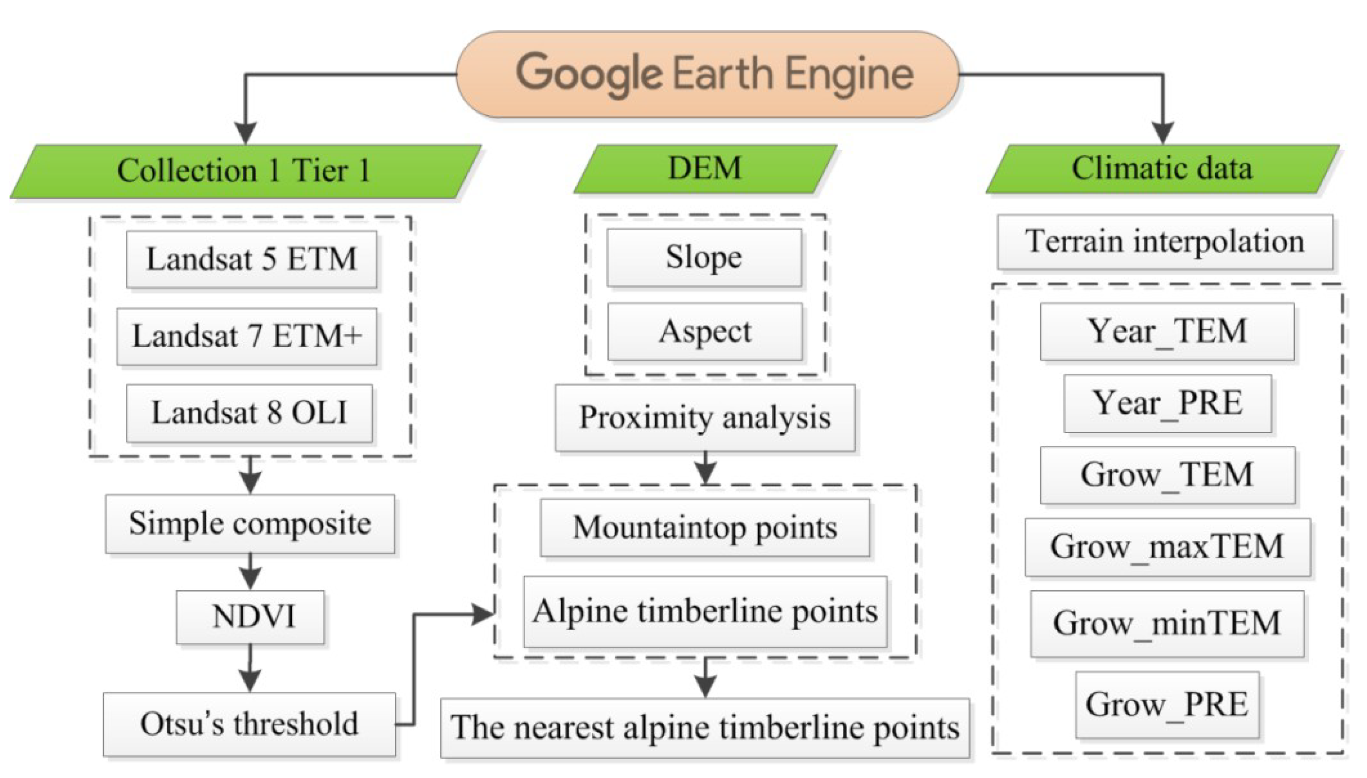
The dynamics of alpine timberline are the result of the interaction of multiple factors. In this study, we chose four hillsides in the western part of Gongga Mountain and acquired the topographic and climatic data at the highest alpine timberline point from 1987–2019 to explore the relationship between alpine timberline, topographic and climatic factors. The west of Gongga Mountain was chosen for its relatively pristine environment conditions and suitable elevation (above 3000 m). We selected a total of 10 factors, including slope, aspect, longitude, latitude, average annual temperature, annual precipitation, growing season temperature, maximum growing season temperature, minimum growing season temperature, and growing season precipitation for each hillside. A combination of Pearson correlation analysis, principal component analysis, and multiple linear regression were performed.
(1) Pearson correlational analysis
The Pearson correlation analysis is a classic mathematical method used to measure the degree of correlation between variables of two groups. The Pearson correlation coefficient quantifies this degree (ranging from −1 to 1) and is calculated as follows:
r = i = 1 n ( x i x ¯ ) ( y i y ¯ ) i = 1 n ( x i x ¯ ) 2 i = 1 n ( y i y ¯ ) 2
where r is the Pearson correlation coefficient, x and y are the variables of the two groups, and n is the number of variables in each group. The variables of the two groups are more closely correlated with absolute values of r closer to 1 [55]. This analysis was performed using the “corrplot” package in the R software (R Core Development Team, R Foundation for Statistical Computing, Vienna, Austria).
(2) Interaction analysis of multiple factors
The principal component analysis (PCA) is a common multivariate method that extracts important information from multidimensional data and visualises principal components in the R software [56]. The number of principal components is determined by the cumulative total variance contribution rate, which should be greater than 75%. Moreover, we used the two R packages “FactoMineR” and “factoextra” to analyse and visualise the data. Multiple linear regression (MLR) is a statistical technique that establishes a linear relationship between explanatory and response variables [57]. The results of the principal components were used as the explanatory variables of MLR in this study.

2.4. Processing

Data processing proceeded as follows (Figure 2): first, we calculated the NDVI of Gongga Mountain from Landsat images in Google Earth Engine. Second, the optimal NDVI thresholds were calculated by the Otsu method, and the threshold pixels were extracted. Next, we limited the alpine timberline points to above 3200 m above sea level and verified the higher alpine timberline points to obtain the final alpine timberline points of Gongga Mountain based on historical Google images, land classification maps, and existing research results [26,32,58]. Then, the nearest alpine timberline points were obtained by seeking the alpine timberline points closest to the mountaintop point in the vicinity of each mountaintop point. After that, we analysed the spatiotemporal dynamic pattern of the nearest alpine timberline points and discussed the distribution of the nearest alpine forest line points on different terrains. Finally, we explored the relationships among the distribution of the highest alpine timberline points and topographic and climatic factors on four different hillsides from 1987–2019.

3. Results

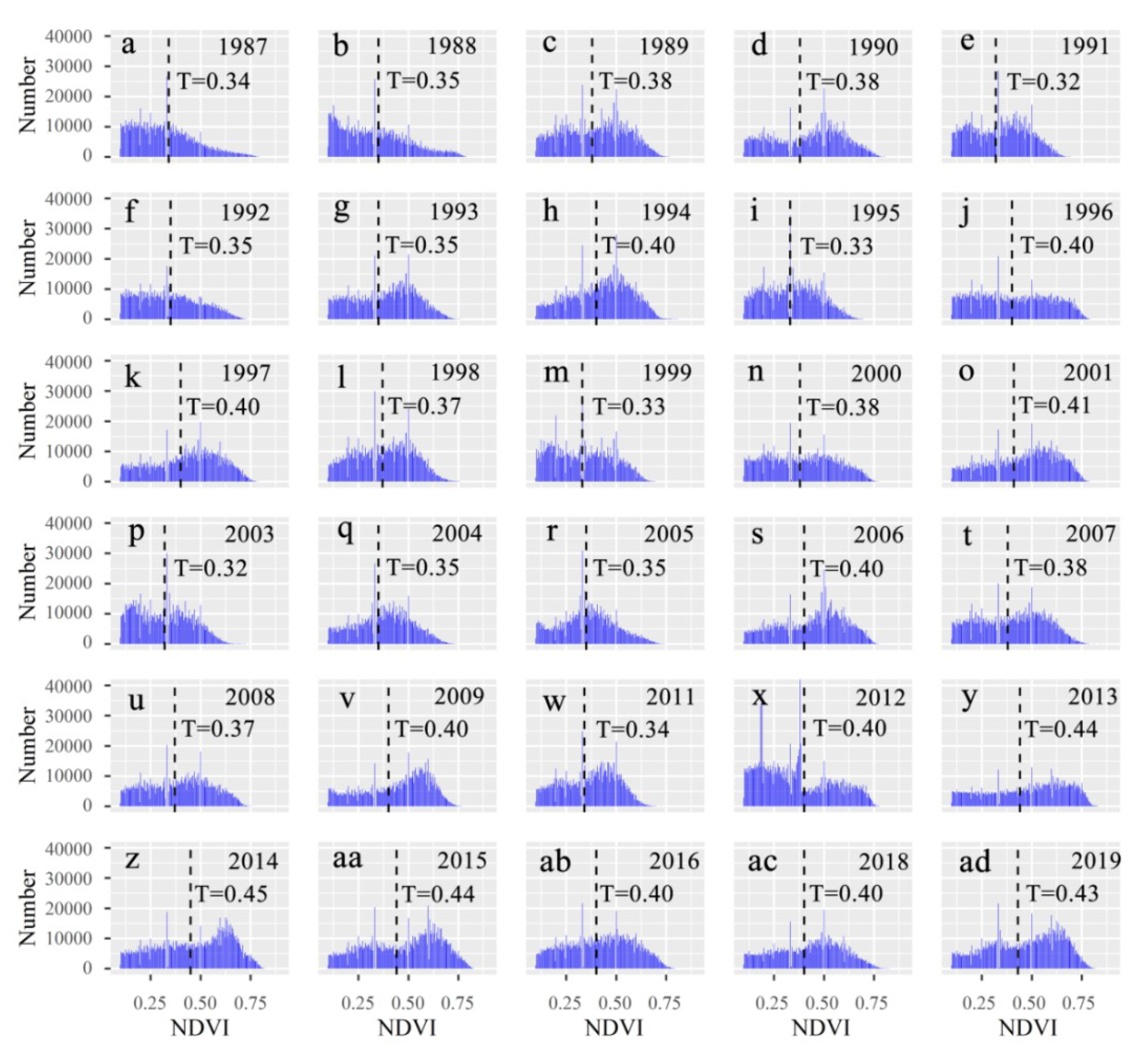
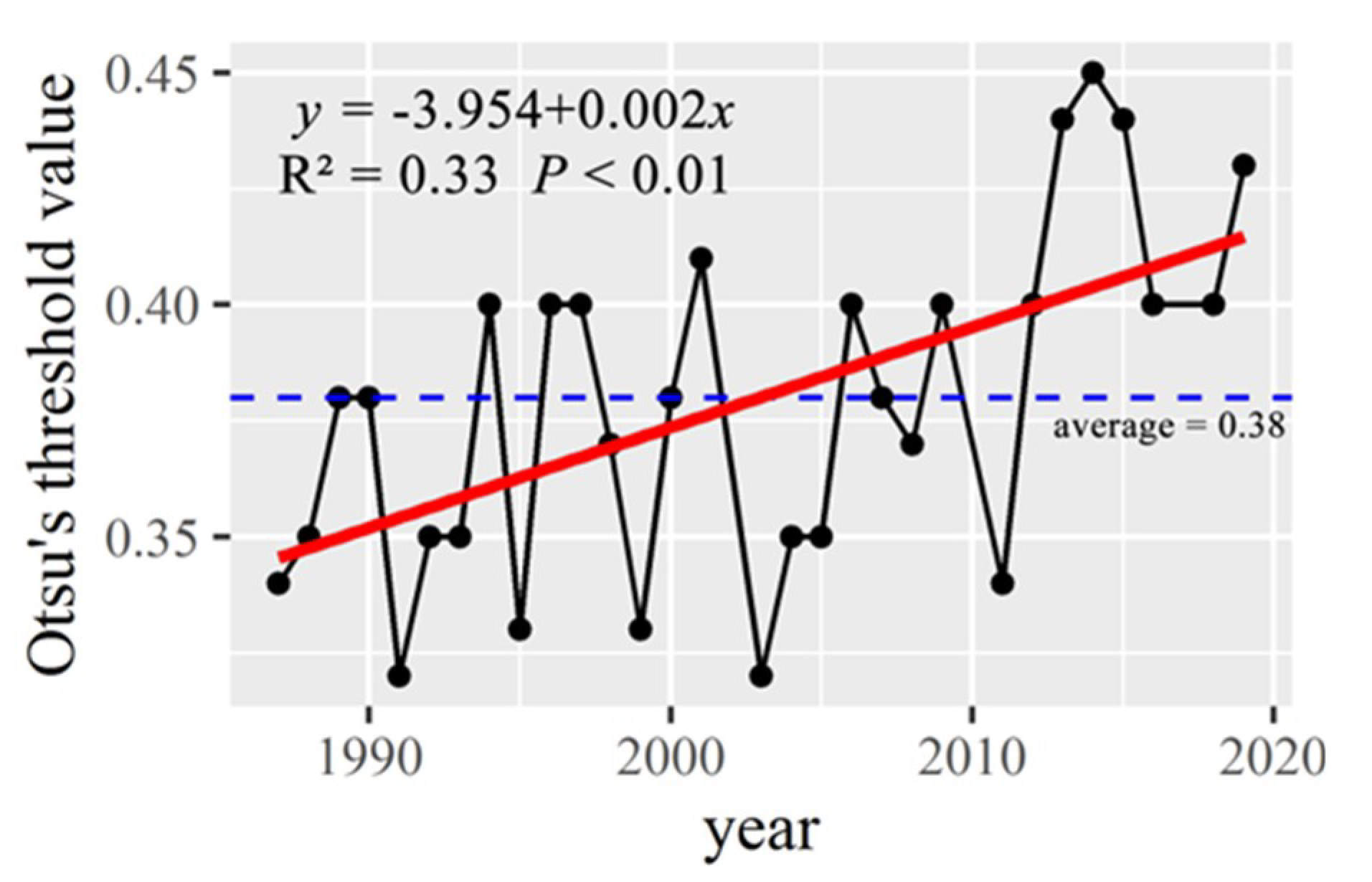
3.1. Otsu Analysis Results

Figure 3 shows the annual Otsu threshold and the NDVI value distribution in the study area. The 30-year average NDVI threshold is 0.38 (Figure 4), and the lowest (Figure 3e) and highest (Figure 3z) NDVI thresholds are 0.32 in 1991 and 0.45 in 2014, respectively. Figure 4 shows the annual Otsu NDVI threshold change. The NDVI threshold of Gongga Mountain has increased significantly (R2 = 0.33, p < 0.01) at a change rate of 0.002/y from 1987–2019 (Figure 4).

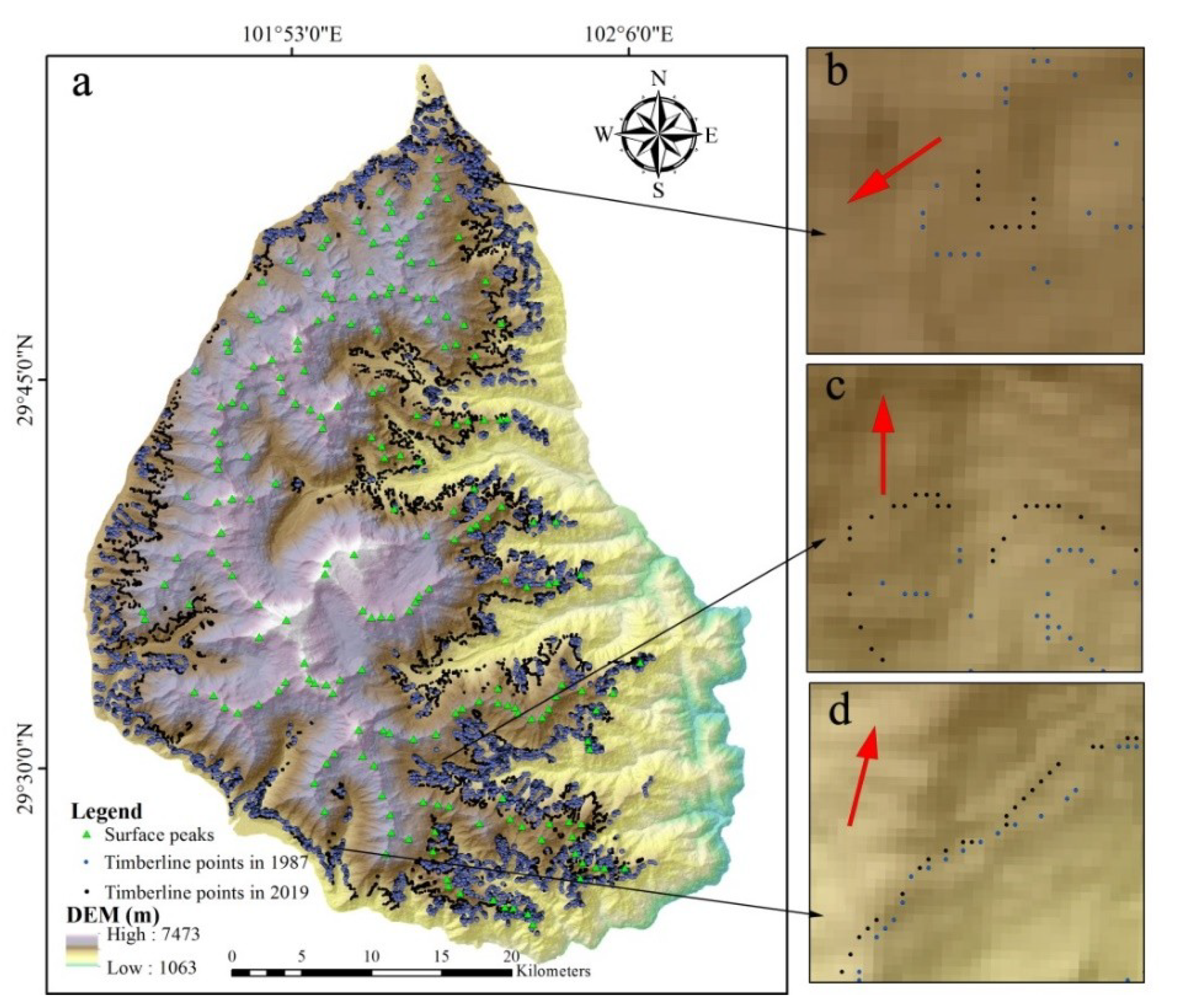
3.2. Spatiotemporal Alpine Timberline Distribution

The height of the alpine timberline rises from 3203 to 4889 m around Gongga Mountain (Figure 5a). There was spatial heterogeneity in dynamics of timberline. There had been a downward, upward, and unobvious trend in the northwest (Figure 5b), southeast (Figure 5c), and southwest (Figure 5d) of Gongga Mountain, respectively.

3.3. Topographic Factors Affecting the Spatial Distribution of the Alpine Timberline

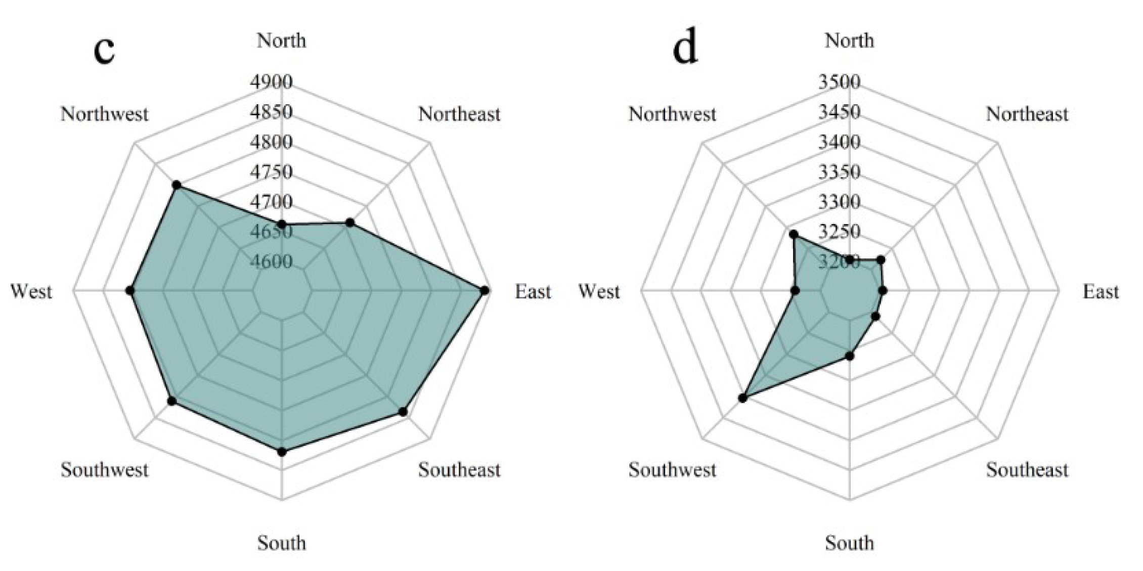
3.3.1. Aspect Factor

The aspect distribution of the alpine timberline points is different on Gongga Mountain (Figure 6). The northeast and west slopes have the highest (901) and lowest (177) number of nearest alpine timberline points, respectively (Figure 6a); the average elevation of the nearest alpine timberline points is highest (4085 m) and lowest (3882 m) on the east and south slopes, respectively (Figure 6b); the highest elevation of the nearest alpine timberline points registers a maximum and minimum on the east (4889 m) and north (4661 m) slopes, respectively (Figure 6c); the lowest elevation of the nearest alpine timberline points registers a maximum and minimum on the east (3404 m) and north (3202 m) slopes, respectively (Figure 6d).

3.3.2. Slope Factor

We performed a statistical distribution of the nearest alpine timberline points on different slope classifications (Figure 7). The distribution of the nearest alpine timberline points is mostly on moderate (15–25°), moderately steep (25–35°), and steep (35–55°) slopes; the steep slope distribution (1347) is the most numerous(Figure 7a); few nearest alpine timberline points are distributed on flat (0–2°), or very gentle (2–5°) slopes with 21 events (Figure 7a). There is no significant difference in the average elevation of the nearest alpine timberline points on different slope classifications (Figure 7b). The maximum elevation of the nearest alpine timberline points is highest and lowest on moderately steep (25–35°) and flat (0–2°) slopes, respectively; the minimum elevation of the nearest alpine timberline points is highest and lowest on flat (0–2°) and steep (35–55°) slopes, respectively.

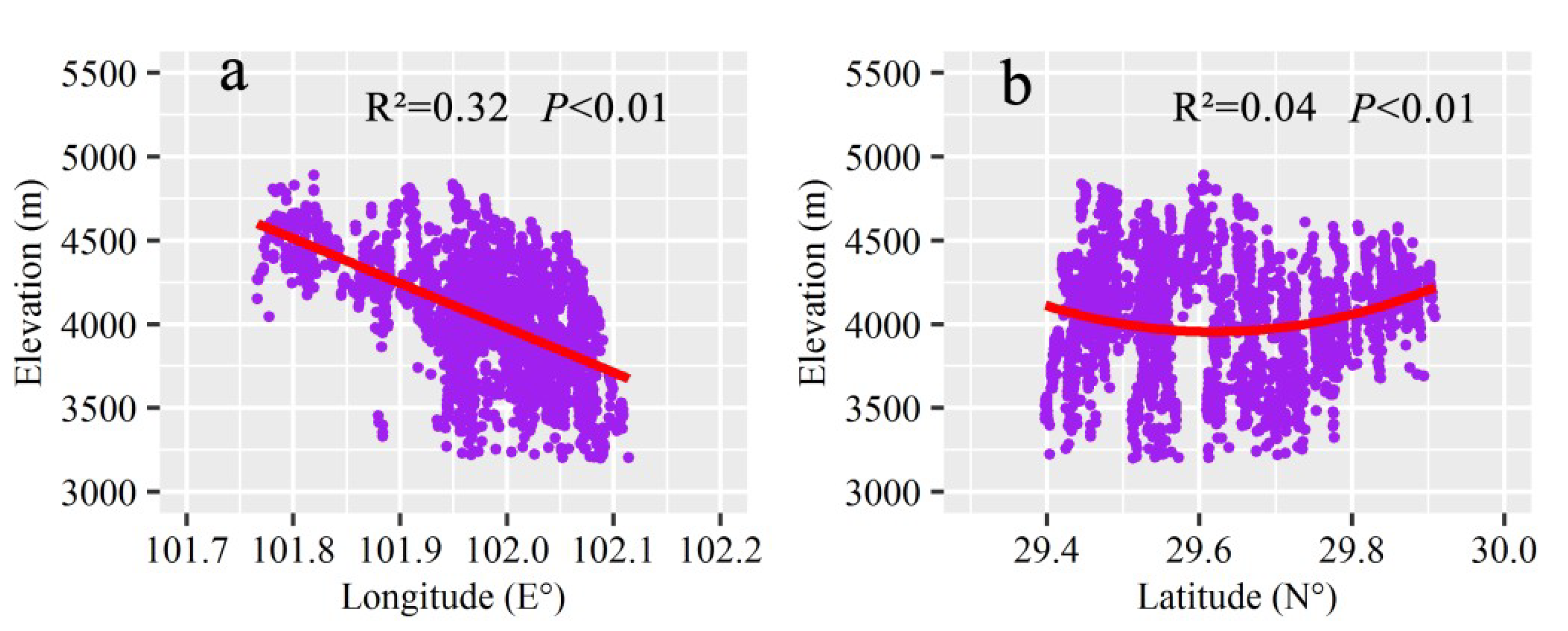
3.3.3. Longitude and Latitude Factors

Figure 8 shows the relationships between the elevation of the nearest alpine timberline points and the longitude and latitude. There was a significant relationship between the longitude and elevation of the alpine timberline (R2 = 0.32, p < 0.01, Figure 8a). Conversely, the relation between latitude and elevation was not significant (binomial fitting: R2 = 0.04, p < 0.01, Figure 8b). The elevation of the alpine timberline points generally drops gradually from west to east (Figure 8a), but the number of alpine timberline points increases from west to east. There are fewer alpine timberline points at high latitudes than at low latitudes (Figure 8b).

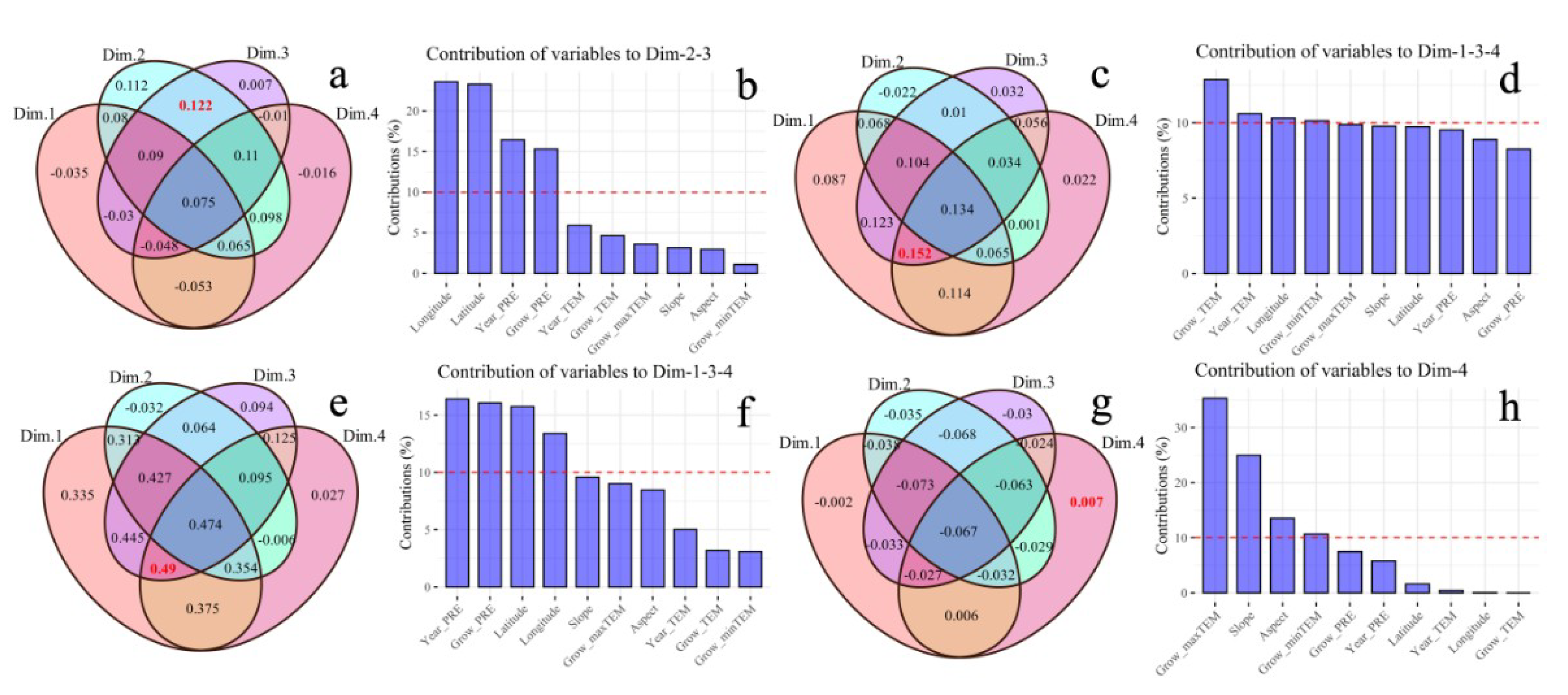
3.4. Driving Factors of the Spatiotemporal Distribution of Alpine Timberlines

On the first hillside, longitude had the highest correlation coefficient with elevation (r = 0.5, p < 0.01, Figure 9a).
According to Figure 10a,b, the highest R2 of MLR was 0.122 based on two principal components (Dim2 and Dim3). Drivers with a greater contribution included longitude, latitude, Year_PRE, and Grow_PRE. Longitude of the second hillside possessed the highest r value with elevation (r = 0.49, p < 0.01), and the factor of the largest negative correlation was slope (r = -0.51, p < 0.01, Figure 9b). The interaction of Dim1, Dim3, and Dim4 contributed the highest R2 value (R2 = 0.152), which accounted for the Grow_TEM, Year_TEM, longitude, and Grow_minTEM (Figure 10c,d). For the third hillside, latitude (r = 0.74, p < 0.01), longitude (r = 0.55, p < 0.01), Grow_PRE (r = 0.52, p < 0.01), and Year_PRE (r = 0.49, p < 0.01) were the principal factors (Figure 9c). The highest R2 value (R2 = 0.49) was a consequence of the interaction of Dim1, Dim3, and Dim4; the principal contributed drivers were Year_PRE, Grow_PRE, latitude, and longitude (Figure 10e,f). The relationship between elevation and aspect factor was most significant on the fourth hillside (r = −0.44, p < 0.05, Figure 9d). The highest R2 value occurred in Dim4, and the critical factors were Grow_maxTEM, slope, aspect, and Grow_minTEM (Figure 10g,h).

4. Discussion

4.1. Temporal and Spatial Dynamics of Alpine Timberline on Gongga Mountain

The elevation of the nearest alpine timberline points to peaks on Gongga Mountain were extracted by remote sensing technology ranges from 3202–4889 m (Figure 5) [48]. The extracted alpine timberline is slightly higher (or lower) than the previous research results on the alpine timberline of the southeastern margin of the Tibetan Plateau (3300–4600 m) [26,31,54,59], which could be attributed to the image resolution (30 m) and DEM vertical accuracy (±12 m). In the last 30 years, the NDVI threshold obtained by the Otsu method has changed significantly (Figure 4), indicating a significant increase in the vegetation coverage near the alpine timberline ecotone. The results are consistent with those of another study that found a significant increase in the population density of Abies fabri near the alpine timberline in the Yajiageng area of Gongga Mountain over the past 100 years [32]. Additionally, some studies showed that the population density of the Smith fir timberline in the southeastern Tibetan Plateau has significantly increased with climate warming since 200 years ago [60]. This also happened in other areas, such as the Spanish Pyrenees and the central Canadian Rockies [61,62]. The harsh environment of the alpine timberline ecotone could affect the shape and size of vegetation but does not affect seed propagation and vegetation regeneration; this fact supports our results [31,60]. The alpine timberline generally shows a slow rising trend, but the rise is not obvious in some areas (Figure 5), indicating the spatial heterogeneity of the alpine timberline. On a global scale, a meta-analysis of 166 datasets showed that 47% of treelines experienced no significant elevation changes [63]. For example, the elevation of alpine timberline did not significantly increase in the Yajiageng area because of growth restricted by grazing [32]. Furthermore, the advance of growing season and the increase of freezing events lead to alpine timberline stability [64,65].
The distribution of alpine timberline points differs on the different aspect. The elevation of the alpine timberline on sunny slopes is generally higher than that of shady slopes (Figure 6), because vegetation receives different solar radiation intensity and duration and heat availability depending on the aspect [66,67]. Additionally, the slope also affects the distribution of alpine timberline (Figure 7). On the one hand, the distribution of alpine timberline points on Gongga Mountain are relatively few in flat and very gentle places (Figure 7a)—because vegetation generally grows better on these slopes. Meanwhile, these flat and extremely gentle slopes are rare on Gongga Mountain (Table 1). On the other hand, fewer alpine timberline points are distributed on very steep slopes (>55°) (Figure 7a), mainly due to the large amount of gravel, scant soil moisture, and unfavorable seed preservation [68,69]. Thus, alpine timberline points are less likely to occur on excessively high or low slopes. The elevation of the alpine timberline decreased from west to east because of the topography of Gongga Mountain—which is higher in the west and lower in the east (Figure 1 and Figure 8a). The latitude in this area had little influence on the distribution of alpine timberline points (Figure 8b), mainly due to the small latitudinal direction span and the complex terrain.

4.2. Drivers Influencing the Spatiotemporal Distribution of the Alpine Timberline

Our findings showed that the drivers of the alpine timberline present spatial heterogeneity on the west slope of Gongga Mountain (Figure 9 and Figure 10). On the first hillside, the longitude has the most significant correlation with the alpine timberline elevation (p < 0.01, Figure 9a); longitude, latitude, Year_PRE, and Grow_PRE exceed the average contribution rate for driving factor interaction (Figure 10b), indicating that longitude is the primary driving factor in this region. However, the alpine timberline migration mechanism must be further observed and studied because of the small terrain span [26]. The contribution rate of Grow_TEM, Year_TEM, longitude, and Grow_minTEM exceeded the average value for driving factor interaction on the second hillside, and precipitation contributed less than average (Figure 10d); slope was the largest negative correlation factor here (p < 0.01, Figure 9b), with increased slopes making water preservation difficult and soil nutrient loss to rainfall more likely, thereby affecting alpine timberline migration [70]. Precipitation is the principal driving force on the third hillside (p < 0.01, Figure 9c and Figure 10e,f). The following reasons explain why precipitation has a significant impact on the alpine timberline; first, precipitation defines the nutrient availability and growth restrictions of vegetation in alpine timberline ecotones [71,72,73]. Second, vegetation possess the limited capacity of precipitation use efficiency on the Tibetan Plateau, leading to wilted seedlings and limited tree growth at high altitudes [74,75,76]. The alpine timberline of the fourth hillside is directly impacted by aspect (p < 0.05, Figure 9d), suggesting that alpine timberlines are constrained by the intensity of solar radiation and sunshine hours, which is consistent with the research results of the timberline ecotone in the Changbai Mountains [77]. Moreover, previous study has shown that the vegetation distribution on Gonga Mountain is controlled by slope [78]. Interestingly, based on the contribution degree, we found that the factors exceeding the average contribution on the first and third hillsides are the same, whereas the factors exceeding the average contribution of the second hillside are completely different to those (Figure 10). Because the first and the third slopes are sunny slopes and the second slope is a shady slope, the alpine timberline differs significantly among these slopes [32]. According to the analysis of these four hillsides, the drivers and migration of the alpine timberline have the hillside differences, and depend on climatic variation and the complex terrain, primarily different hydrothermal conditions, which affects the inconsistency of vegetation growth [79,80].
We conducted a literature survey addressing drivers of alpine timberline (Table 3). Regional differences of driving factors show dissimilarly dynamics of alpine timberline, but water and heat are the most basic factors affecting the alpine timberline. The accelerated retreat of glaciers caused by climate warming; this could lead to a more significant upward alpine timberline trend on Gongga Mountain [81,82]. However, species interactions may prevent the migration of the alpine timberline to higher elevations of the Tibetan Plateau [83]. Predicting and simulating alpine timberline dynamics is increasingly difficult because of the frequency of extreme weather, human activities and the lagging and diverse response of the alpine timberline to climate change [84,85,86]. Therefore, a combination of biotic and abiotic factors should be considered when predicting and simulating alpine timberline migration.

4.3. Importance and Uncertainties

In this study, the Otsu method was used to extract the alpine timberline on the spatial scale that based on the Google Earth Engine and calculate the Otsu threshold of NDVI across the Gongga Mountain during 1987–2019, which captured alpine timberline variation on the pixel level and discussed the drivers of alpine timberline. The Otsu method is very adaptable to different time scales, and regions, and it can also confirm the optimal threshold of alpine timberline. For the extracting alpine timberline, we selected images derived from the early growing season, which can capture the growth characteristics of different vegetation types based on the differences of NDVI. Additionally, the ASTER GDEM V3, highly accurate DEM, was introduced to calculate the elevation of alpine timberline [48], which can improve the identification accuracy of alpine timberline. As we known, the climate is easily affected by the complicated topography, which is indispensable datasets for studying the drivers of alpine timberline; fortunately, the Anusplin 4.2 software is good tool which can improve the spatial interpolations accuracy in term of variations of topography. Moreover, Google Earth Engine provides better opportunities for undertaking alpine timberline observation studies because of its huge datasets and efficient computing power [42,43]. Ultimately, the drivers of different hillsides highlighted the different response processes and mechanisms of alpine timberline on spatial scale, which is helpful for future studies regarding the effect of climate change and topography on dynamics of alpine timberline.
Despite we obtained a certain achievement, the difference in the spectral bands and the instrument performances between Landsat 8 OLI and Landsat-5 TM/Landsat-7 ETM+ might cause inconsistency on the derived NDVI [94,95]. However, some studies have shown that NDVIs of Landsat 8 OLI and Landsat-7 ETM+ have good consistency, especially for vegetation types, they have better NDVI consistency than non-vegetation types [96,97]. Besides, it is significant challenges to extract alpine timberline on the pixel level with vegetation composites in thematic map because of the quality and the uneven availability of Landsat images at spatiotemporal scales [98,99]. Consequently, we checked multi-year alpine timberline maps by historical Google images, land classification maps, and existing research results, and minimized the uncertainties that derived from the data availability. Furthermore, vertical and horizontal errors in the DEM could led to the overall uncertainty for the alpine timberline elevation. In our study, the compounded dynamic mechanism study of timberline is scarce due to the limitation of data. Thus, we used previous research to explain our results, and the specific in situ observation should be considered in the future. If additional data becomes available, further studies will be conducted to evaluate the performance of the Landsat maps with alpine timberline elevation, density and future trend at the sub-pixel scale.

5. Conclusions

Alpine timberlines are warning signal and amplifier of global change. Remote sensing and geographic information system are the most essential tools for studying alpine timberline dynamics. In this research, we emphasized that the alpine timberline is an ecosystem ecotone rather than a vegetation type boundary. We used the Otsu method to extract the alpine timberline on Google Earth Engine, analysed the spatiotemporal pattern of the alpine timberline, and detected the controls of alpine timberline using Pearson’s correlation coefficient, MLR, and PCA. Our results suggested that the vegetation coverage near the alpine timberline increases notable. The alpine timberline rose slowly with insignificant change in some areas and is controlled by aspect, slope, longitude, and latitude. The drives of alpine timberline had spatial heterogeneity on Gongga Mountain. Notable differences exist on sunny and shady slopes of alpine timberline. Consequently, more attention should be devoted to monitoring and simulating dynamics of alpine timberline on different hillsides. Additionally, the physical and chemical properties of soil and vegetation traits should be investigated in the field to better monitor the changed mechanisms of alpine timberline and to further deepen the understanding of the linkage of the alpine ecotone with climate change.

Author Contributions

Conceptualization, J.S. and W.H.; methodology, W.H.; software, W.H.; validation, J.S. and W.H.; formal analysis, W.H.; investigation, W.H.; resources, J.X.; data curation, J.S.; writing—original draft preparation, W.H.; writing—review and editing, C.Y., J.X., J.W. and T.Z.; visualization, W.H.; supervision, J.S.; project administration, J.S.; funding acquisition, J.S. and J.X. All authors have read and agreed to the published version of the manuscript.

Funding

This research was supported by the Second Tibetan Plateau Scientific Expedition and Research (Grant No. 2019QZKK0405), the National Science Foundation of China (No.41661144045 and 31971436), Strategic Priority Research Program of the Chinese Academy of Sciences (Grant No. XDA20030302), and the Science and Technology Project of Xizang Autonomous Region (Grant No. XZ201901-GA-07).

Conflicts of Interest

The authors declare no conflict of interest.

References

  1. Gonzalez, P.; Neilson, R.P.; Lenihan, J.M.; Drapek, R.J. Global patterns in the vulnerability of ecosystems to vegetation shifts due to climate change. Glob. Ecol. Biogeogr. 2010, 19, 755–768. [Google Scholar] [CrossRef]
  2. Jimenez, M.A.; Jaksic, F.M.; Armesto, J.J.; Gaxiola, A.; Meserve, P.L.; Kelt, D.A.; Gutierrez, J.R. Extreme climatic events change the dynamics and invasibility of semi-arid annual plant communities. Ecol. Lett. 2011, 14, 1227–1235. [Google Scholar] [CrossRef] [PubMed]
  3. Mayor, J.R.; Sanders, N.J.; Classen, A.T.; Bardgett, R.D.; Clement, J.C.; Fajardo, A.; Lavorel, S.; Sundqvist, M.K.; Bahn, M.; Chisholm, C.; et al. Elevation alters ecosystem properties across temperate treelines globally. Nature 2017, 542, 91–95. [Google Scholar] [CrossRef] [Green Version]
  4. Janetos, A.C.; Watson, R.T.; Zinyowera, M.C.; Moss, R.H. Climate change 1995: Impacts, adaptations and mitigation of climate change: Scientific-technical analyses. Ecology 1997, 78, 465–477. [Google Scholar] [CrossRef]
  5. Fang, J.Y.; Piao, S.L.; He, J.H.; Ma, W.H. Increasing terrestrial vegetation activity in China, 1982–1999. Sci. China Ser. C Life Sci. 2004, 47, 229–240. [Google Scholar]
  6. Wu, Z.T.; Wu, J.J.; He, B.; Liu, J.H.; Wang, Q.F.; Zhang, H.; Liu, Y. Drought offset ecological restoration program-induced increase in vegetation activity in the Beijing-Tianjin Sand Source Region, China. Environ. Sci. Technol. 2014, 48, 12108–12117. [Google Scholar] [CrossRef]
  7. Myneni, R.B.; Keeling, C.D.; Tucker, C.J.; Asrar, G.; Nemani, R.R. Increased plant growth in the northern high latitudes from 1981 to 1991. Nature 1997, 386, 698–702. [Google Scholar] [CrossRef]
  8. Myers-Smith, I.H.; Forbes, B.C.; Wilmking, M. Shrub encroachment in arctic and alpine tundra: Dynamics, impacts and research priorities. Environ. Res. Lett. 2011, 6, 1–15. [Google Scholar] [CrossRef] [Green Version]
  9. Mclaren, J.R.; Buckeridge, K.M.; Weg, M.J.V.D.; Shaver, G.R.; Schimel, J.P.; Gough, L. Shrub encroachment in Arctic tundra: Betula nana effects on above-and belowground litter decomposition. Ecology 2017, 98, 1361–1376. [Google Scholar] [CrossRef] [Green Version]
  10. Urbina-Cardona, J.N.; Olivares-Pérez, M.; Reynoso, V.H. Herpetofauna diversity and microenvironment correlates across a pasture–edge–interior ecotone in tropical rainforest fragments in the Los Tuxtlas Biosphere Reserve of Veracruz, Mexico. Biol. Conserv. 2006, 132, 0–75. [Google Scholar] [CrossRef]
  11. Dutoit, T.; Buisson, E.; Gerbaud, E.; Roche, P.; Tatoni, T. The status of transitions between cultivated fields and their boundaries: Ecotones, ecoclines or edge effects? Acta Oecol. 2007, 31, 0–136. [Google Scholar] [CrossRef]
  12. Holtmeier, F.K. Mountain Timberlines—Ecology, Patchiness, And Dynamics; Springer: Berlin, Germany, 2009. [Google Scholar]
  13. Tranquillini, W. Physiological Ecology of the Alpine Timberline; Springer: Berlin/Heidelberg, Germany, 1979. [Google Scholar]
  14. Korner, C. Treelines will be understood once the functional difference between a tree and a shrub is. Ambio 2012, 41, 197–206. [Google Scholar] [CrossRef] [PubMed] [Green Version]
  15. Lloyd, A.H.; Fastie, C.L. Spatial and temporal variability in the growth and climate response of treeline trees in Alaska. Clim. Chang. 2002, 52, 481–509. [Google Scholar] [CrossRef]
  16. Sitko, I.; Troll, M. Timberline Changes in relation to summer farming in the Western Chornohora (Ukrainian Carpathians). Mt. Res. Dev. 2008, 28, 263–271. [Google Scholar] [CrossRef] [Green Version]
  17. Singh, C.; Panigrahy, S.; Thapliyal, A.; Kimothi, M.; Soni, P.; Parihar, J. Monitoring the alpine treeline shift in parts of the Indian Himalayas using remote sensing. Curr. Sci. 2012, 102, 559–562. [Google Scholar]
  18. Kumar, M.; Kumar, P. Snow cover dynamics and timberline change detection of Yamunotri watershed using multi-temporal satellite imagery. In Climate Change, Glacier Response, and Vegetation Dynamics in the Himalaya: Contributions Toward Future Earth Initiatives; Singh, R.B., Schickhoff, U., Mal, S., Eds.; Springer International Publishing: Cham, Switzerland, 2016; pp. 391–399. [Google Scholar]
  19. Theurillat, J.P.; Guisan, A. Potential impact of climate change on vegetation in the European Alps: A review. Clim. Chang. 2001, 50, 77–109. [Google Scholar] [CrossRef]
  20. Smith, M. Alpine treelines: Functional ecology of the global high elevation tree limits. Mt. Res. Dev. 2013, 33, 357. [Google Scholar] [CrossRef]
  21. Korner, C. The use of ‘altitude‘ in ecological research. Trends Ecol. Evol. 2007, 22, 569–574. [Google Scholar] [CrossRef]
  22. Körner, C.; Paulsen, J. World-wide study of high altitude treeline temperatures. J. Biogeogr. 2004, 31, 713–732. [Google Scholar] [CrossRef]
  23. Rupp, T.S.; Chapin, I.I.I.F.S.; Starfield, A.M. Modeling the influence of topographic barriers on treeline advance at the forest-tundra ecotone in Northwestern Alaska. Clim. Chang. 2001, 48, 399–416. [Google Scholar] [CrossRef]
  24. Wang, M.; Li, Y.; Huang, R.Q.; Li, Y.L. The effects of climate warming on the alpine vegetation of the Qinghai-Tibetan Plateau hinterland. Acta Ecol. Sin. 2005, 25, 1275–1281. [Google Scholar]
  25. MacDonald, G.M.; Kremenetski, K.V.; Beilman, D.W. Climate change and the northern Russian treeline zone. Philos. Trans. Biol. Sci. 2008, 363, 2285–2299. [Google Scholar] [CrossRef] [PubMed] [Green Version]
  26. Wang, X.P.; Zhang, L.; Fang, J.Y. Geographical differences in alpine timberline and its climatic interpretation in China. Acta Geogr. Sin. 2004, 59, 871–879. [Google Scholar]
  27. Grigor’ev, A.A.; Moiseev, P.A.; Nagimov, Z.Y. Dynamics of the timberline in high mountain areas of the nether-polar Urals under the influence of current climate change. Russ. J. Ecol. 2013, 44, 312–323. [Google Scholar] [CrossRef]
  28. Valmore, C.L.; Harold, A.M. Recent climatic change and development of the bristlecone pine (P. Longaeva bailey) Krummholz zone, Mt. Washington, Nevada. Arct. Alp. Res. 2018, 4, 61–72. [Google Scholar]
  29. Zhou, T.Y.; Narayan, P.G.; Liao, L.B.; Zheng, L.L.; Wang, J.N.; Sun, J.; Wei, Y.Q.; Xie, Y.; Wu, Y. Spatio-temporal dynamics of two alpine treeline ecotones and ecological characteristics of their dominate species at the eastern margin of Qinghai-Xizang Plateau. Chin. J. Plant Ecol. 2018, 42, 1082–1093. [Google Scholar] [CrossRef] [Green Version]
  30. Huo, C.F.; Cheng, G.W.; Lu, X.Y.; Fan, J.H. Simulating the effects of climate change on forest dynamics on Gongga Mountain, Southwest China. J. For. Res. 2010, 15, 176–185. [Google Scholar] [CrossRef]
  31. Shen, Z.H.; Fang, J.Y.; Liu, Z.L.; Wu, J. Structure and dynamics of Abies Fabri population near the Alpine timberline in Hailuo Clough of Gongga Mountain. Acta Bot. Sin. 2001, 1288–1293. [Google Scholar]
  32. Ran, F.; Liang, Y.M.; Yang, Y.; Yang, Y.; Wang, G.X. Spatial-temporal dynamics of an Abies fabri population near the alpine treeline in the Yajiageng area of Gongga Mountain, China. Acta Ecol. Sin. 2014, 34, 6872–6878. [Google Scholar]
  33. Hill, R.; Granica, K.; Smith, G.; Schardt, M. Representation of an alpine treeline ecotone in SPOT 5 HRG data. Remote Sens. Environ. 2007, 110, 458–467. [Google Scholar] [CrossRef]
  34. Panigrahy, S.; Anitha, D.; Kimothi, M.M.; Singh, S.P. Timberline change detection using topographic map and satellite. Trop. Ecol. 2010, 51, 87–91. [Google Scholar]
  35. Mohapatra, J.; Singh, C.P.; Tripathi, O.P.; Pandya, H.A. Remote sensing of alpine treeline ecotone dynamics and phenology in Arunachal Pradesh Himalaya. Int. J. Remote Sens. 2019, 40, 7986–8009. [Google Scholar] [CrossRef]
  36. Zhang, Y.J.; Xu, M.; Adams, J.; Wang, X.C. Can Landsat imagery detect tree line dynamics? Int. J. Remote Sens. 2009, 30, 1327–1340. [Google Scholar] [CrossRef]
  37. Bharti, R.R.; Adhikari, B.S.; Rawat, G.S. Assessing vegetation changes in timberline ecotone of Nanda Devi National Park, Uttarakhand. Int. J. Appl. Earth Observ. Geoinf. 2012, 18, 472–479. [Google Scholar] [CrossRef]
  38. Rai, I.D.; Bharti, R.R.; Adhikari, B.S.; Rawat, G.S. Structure and Functioning of Timberline Vegetation in the Western Himalaya: A Case Study; International Centre for Integrated Mountain Development: Kathmandu, Nepal, 2013. [Google Scholar]
  39. Otsu, N. A Threshold selection method from gray-level histograms. IEEE Trans. Syst. Man 2007, 9, 62–66. [Google Scholar] [CrossRef] [Green Version]
  40. Li, Y.G.; Chen, G.Q.; Han, Z.; Zheng, L.; Zhang, F.L. A hybrid automatic thresholding approach using panchromatic imagery for rapid mapping of landslides. GISci. Remote Sens. 2014, 51, 710–730. [Google Scholar] [CrossRef]
  41. Ratnakumar, R.; Nanda, S.J. A low complexity hardware architecture of K-means algorithm for real-time satellite image segmentation. Multimed. Tools Appl. 2018, 78, 11949–11981. [Google Scholar] [CrossRef]
  42. Moore, R.T.; Hansen, M.C. Google Earth Engine: A New Cloud-Computing Platform for Global-Scale Earth Observation Data and Analysis. Available online: https://ui.adsabs.harvard.edu/abs/2011AGUFMIN43C..02M (accessed on 20 December 2019).
  43. Gorelick, N.; Hancher, M.; Dixon, M.; Ilyushchenko, S.; Thau, D.; Moore, R. Google Earth Engine: Planetary-scale geospatial analysis for everyone. Remote Sens. Environ. 2017, 202, 18–27. [Google Scholar] [CrossRef]
  44. Lu, X.Y.; Cheng, G.W. Climate change effects on soil carbon dynamics and greenhouse gas emissions in Abies fabri forest of subalpine, southwest China. Soil Biol. Biochem. 2009, 41, 1015–1021. [Google Scholar] [CrossRef]
  45. Yu, L.; Song, M.Y.; Lei, Y.B.; Duan, B.L.; Berninger, F.; Korpelainen, H.; Niinemets, Ü.; Li, C.Y. Effects of phosphorus availability on later stages of primary succession in Gongga Mountain glacier retreat area. Environ. Exp. Bot. 2017, 141, 103–112. [Google Scholar] [CrossRef] [Green Version]
  46. Sun, J.; Cheng, G.W. Mountain Altitudinal Belt: A Review. Ecol. Environ. Sci. 2014, 23, 1544–1550. [Google Scholar]
  47. Eric, V.; Chris, J.; Martin, C.; Belen, F. Preliminary analysis of the performance of the Landsat 8/OLI land surface reflectance product. Remote Sens. Environ. 2016, 185, 46–56. [Google Scholar]
  48. Abrams, M.; Crippen, R.; Fujisada, H. ASTER Global Digital Elevation Model (GDEM) and ASTER Global Water Body Dataset (ASTWBD). Remote Sens. 2020, 12, 1156. [Google Scholar] [CrossRef] [Green Version]
  49. Clinton, N. Otsu’s Method for Image Segmentation. Available online: https://medium.com/google-earth/otsus-method-for-image-segmentation-f5c48f405e (accessed on 10 January 2020).
  50. Torres-Sánchez, J.; López-Granados, F.; Peña, J.M. An automatic object-based method for optimal thresholding in UAV images: Application for vegetation detection in herbaceous crops. Comput. Electron. Agric. 2015, 114, 43–52. [Google Scholar] [CrossRef]
  51. Donchyts, G.; Baart, F.; Winsemius, H.; Gorelick, N.; Kwadijk, J.; van de Giesen, N. Earth‘s surface water change over the past 30 years. Nat. Clim. Chang. 2016, 6, 810–813. [Google Scholar] [CrossRef]
  52. Piao, S.L.; Fang, J.Y.; Ji, W.; Guo, Q.H.; Ke, J.H.; Tao, S. Variation in a satellite-based vegetation index in relation to climate in China. J. Veg. Sci. 2004, 15, 219–226. [Google Scholar] [CrossRef]
  53. Piao, S.L.; Wang, X.H.; Ciais, P.; Zhu, B.; Wang, T.; Liu, J. Changes in satellite-derived vegetation growth trend in temperate and boreal Eurasia from 1982 to 2006. Glob. Chang. Biol. 2011, 17, 3228–3239. [Google Scholar] [CrossRef]
  54. Jiang, L.G.; Liu, X.N.; Feng, Z.M. Remote sensing identification and spatial pattern analysis of the alpine timberline in the three parallel rivers region. Resour. Sci. 2014, 36, 259–266. [Google Scholar]
  55. Xiong, J.N.; Ye, C.C.; Cheng, W.M.; Guo, L.; Zhou, C.H.; Zhang, X.L. The spatiotemporal distribution of flash floods and analysis of partition driving forces in Yunnan Province. Sustainability 2019, 11, 2926. [Google Scholar] [CrossRef] [Green Version]
  56. Abdi, H.; Williams, L.J. Principal component analysis. Wiley Interdiscip. Rev. Comput. Stat. 2010, 2, 433–459. [Google Scholar] [CrossRef]
  57. Uyanık, G.K.; Güler, N. A Study on Multiple Linear Regression Analysis. Procedia Soc. Behav. Sci. 2013, 106, 234–240. [Google Scholar] [CrossRef] [Green Version]
  58. Zhu, W.Z.; Ran, F.; Li, M.H.; Wang, W.Z.; Jia, M. Alpine timberline dynamics and physiological mechanisms of the timberline formation on the Mt.Gongga. Mt. Res. 2017, 35, 622–628. [Google Scholar]
  59. Li, P. Study of Physiological Characteristics of the Alpine Treeline Trees in Mt. Gongga, Southwest China. Master’s Thesis, Southwest University, Chongqing, China, 2008. [Google Scholar]
  60. Liang, E.Y.; Wang, Y.F.; Eckstein, D. Little change in the fir tree-line position on the southeastern Tibetan Plateau after 200 years of warming. New Phytol. 2011, 190, 760–769. [Google Scholar] [CrossRef] [PubMed]
  61. Camarero, J.J.; Gutiérrez, E. Pace and pattern of recent treeline dynamics: Response of ecotones to climatic variability in the Spanish Pyrenees. Clim. Chang. 2004, 63, 181–200. [Google Scholar] [CrossRef]
  62. Macdonald, G.M.; Szeicz, J.M.; Dale, C.K.A. Response of the Central Canadian Treeline to recent climatic changes. Ann. Assoc. Am. Geogr. 1998, 88, 183–208. [Google Scholar] [CrossRef]
  63. Harsch, M.A.; Hulme, P.E.; McGlone, M.S.; Duncan, R.P. Are treelines advancing? A global meta-analysis of treeline response to climate warming. Ecol. Lett. 2009, 12, 1040–1049. [Google Scholar] [CrossRef]
  64. Shen, W.; Zhang, L.; Guo, Y.; Luo, T.X. Causes for treeline stability under climate warming: Evidence from seed and seedling transplant experiments in southeast Tibet. For. Ecol. Manag. 2018, 408, 45–53. [Google Scholar] [CrossRef]
  65. Zhang, G.L.; Zhang, Y.J.; Dong, J.W.; Xiao, X.M. Green-up dates in the Tibetan Plateau have continuously advanced from 1982 to 2011. Proc. Natl. Acad. Sci. USA 2013, 110, 4309–4314. [Google Scholar] [CrossRef] [Green Version]
  66. Dubayah, R.C. Modeling a solar radiation topoclimatology for the Rio Grande River Basin. J. Veg. Sci. 1994, 5, 627–640. [Google Scholar] [CrossRef]
  67. Li, X.; Huang, J.F.; Wang, X.Z. Temporal and spatial distribution characteristics of sunshine duration based on GIS in mountainous areas. Trans. Chin. Soc. Agric. Eng. 2006, 22, 108–113. [Google Scholar]
  68. Lambert, M.S.; Mariam, T.T.; Susan, F.H. Vegetation and Slope Stability; Betascript Publishing: Beau Bassin, Mauritius, 2010. [Google Scholar]
  69. Weltzin, J.F.; Allen, P.B. Tree Seedling Recruitment in a Temperate Deciduous Forest: Interactive Effects of Soil Moisture, Light, and Slope Position; Springer: New York, NY, USA, 2003. [Google Scholar]
  70. Dou, X.L.; Li, M.; Wang, W.B.; Zhang, Q.F.; Cheng, X.L. Changes in soil nutrients in different eroded soils in Pinus massoniana forest ecosystems in Fujian Province, China. Plant Sci. J. 2012, 30, 161–168. [Google Scholar] [CrossRef]
  71. Gilfedder, L. Factors influencing the maintenance of an inverted Eucalyptus coccifera tree-line on the Mt Wellington Plateau, Tasmania. Aust. J. Ecol. 1988, 13, 495–503. [Google Scholar] [CrossRef]
  72. Huxman, T.; Smith, M.D.; Fay, P.A.; Knapp, A.K.; Shaw, M.R.; Loik, M.E.; Smith, S.D.; Tissue, D.T.; Zak, J.C.; Weltzin, J.F.; et al. Convergence across biomes to a common rain-use efficiency. Nature 2004, 429, 651–654. [Google Scholar] [CrossRef] [PubMed]
  73. Wei, S.S.; Wang, Y.; Yu, F. Research advances in key factors affecting seedling regeneration above treeline. Chin. J. Ecol. 2019, 38, 3535–3541. [Google Scholar]
  74. Zhou, T.C.; Liu, M.; Sun, J.; Li, Y.R.; Shi, P.L.; Tsunekawa, A.; Zhou, H.K.; Yi, S.H.; Xue, X. The patterns and mechanisms of precipitation use efficiency in alpine grasslands on the Tibetan Plateau. Agric. Ecosyst. Environ. 2020, 292, 106833–106843. [Google Scholar] [CrossRef]
  75. Qi, Z.M.; Wang, K.Y. On soil water characteristics of the subalpine timberline ecotone and adjacent vegetations in Western Sichuan. J. Southwest China Norm. Univ. (Nat. Sci. Ed.) 2013, 38, 90–95. [Google Scholar]
  76. Ehleringer, J. Physiological Ecology of North American Plant Communities; Chapman and Hall: Dordrecht, The Netherlands, 1985. [Google Scholar]
  77. Zong, S.W.; Wu, Z.F.; Xu, J.W.; Li, M.; Gao, X.F.; He, H.S.; Du, H.B.; Wang, L. Current and potential tree locations in tree line ecotone of Changbai Mountains, Northeast China: The controlling effects of topography. PLoS ONE 2014, 9, e106114. [Google Scholar] [CrossRef] [Green Version]
  78. Shen, Z.H.; Liu, Z.L.; Fang, J.Y. Altitudinal changes in species diversity and community structure of Abies fabri communities at Hailuo Valley of Mt.Gongga, Sichuan. Biodivers. Sci. 2004, 12, 237–244. [Google Scholar]
  79. Gallardo-Cruz, J.A.; Pérez-García, E.A.; Meave, J.A. β-Diversity and vegetation structure as influenced by slope aspect and altitude in a seasonally dry tropical landscape. Landsc. Ecol. 2009, 24, 473–482. [Google Scholar] [CrossRef]
  80. Cheng, G.W. Exploration of precipitation features on extra-high zone of Mt. Gongga. Mt. Res. 1996, 14, 177–182. [Google Scholar]
  81. Cao, B.; Pan, B.T.; Guan, W.J.; Wen, Z.L.; Wang, J. Changes in glacier volume on Mt. Gongga, southeastern Tibetan Plateau, based on the analysis of multi-temporal DEMs from 1966 to 2015. J. Glaciol. 2019, 65, 366–375. [Google Scholar] [CrossRef] [Green Version]
  82. Liao, H.J.; Liu, Q.; Zhong, Y.; Lu, X.Y. Landsat-based estimation of the glacier surface temperature of Hailuogou glacier, Southeastern Tibetan Plateau, between 1990 and 2018. Remote Sens. 2020, 12, 2105. [Google Scholar] [CrossRef]
  83. Liang, E.Y.; Wang, Y.F.; Piao, S.L.; Lu, X.M.; Camarero, J.J.; Zhu, H.F.; Zhu, L.P.; Ellison, A.M.; Ciais, P.; Penuelas, J. Species interactions slow warming-induced upward shifts of treelines on the Tibetan Plateau. Proc. Natl. Acad. Sci. USA 2016, 113, 4380–4385. [Google Scholar] [CrossRef] [PubMed] [Green Version]
  84. Xiong, J.N.; Yong, Z.W.; Wang, Z.G.; Cheng, W.M.; Li, Y.; Zhang, H.; Ye, C.C.; Yang, Y.M. Spatial and temporal patterns of the extreme precipitation across the Tibetan Plateau (1986–2015). Water 2019, 11, 1453. [Google Scholar] [CrossRef] [Green Version]
  85. Fang, J.Q.; Wu, N.; Luo, P.; Yi, S.L. Impacts of disturbances on alpine timberline reformation. Chin. J. Ecol. 2005, 24, 1493–1498. [Google Scholar]
  86. Van Bogaert, R.; Haneca, K.; Hoogesteger, J.; Jonasson, C.; De Dapper, M.; Callaghan, T.V. A century of tree line changes in sub-Arctic Sweden shows local and regional variability and only a minor influence of 20th century climate warming. J. Biogeogr. 2011, 38, 907–921. [Google Scholar] [CrossRef] [Green Version]
  87. Chhetri, P.K.; Shrestha, K.B.; Cairns, D.M. Topography and human disturbances are major controlling factors in treeline pattern at Barun and Manang area in the Nepal Himalaya. J. Mt. Sci. 2017, 14, 119–127. [Google Scholar] [CrossRef]
  88. Schickhoff, U.; Bobrowski, M.; Böhner, J.; Bürzle, B.; Schwab, N. Climate Change and Treeline Dynamics in the Himalaya; Springer International Publishing: Cham, Switzerland, 2016. [Google Scholar]
  89. Kaczka, R.J.; Czajka, B.; Łajczak, A. The tree-ring growth responses to climate in the timberline ecotone of Babia Góra Mountain. Geogr. Pol. 2015, 88, 163–176. [Google Scholar] [CrossRef] [Green Version]
  90. Kaczka, R.J.; Czajka, B.; Łajczak, A.; Szwagrzyk, J.; Nicia, P. The timberline as result of the interactions among forest, abiotic environment and human activity in the Babia Góra Mt., Western Carpathians. Geogr. Pol. 2015, 88, 177–191. [Google Scholar] [CrossRef] [Green Version]
  91. Lioyd, A.H.; Graumlich, L.J. Holocene dynamics of treeline forests in the sierra nevada. Ecology 1997, 78, 1199–1210. [Google Scholar] [CrossRef]
  92. Sullivan, P.F.; Sveinbjörnsson, B. Microtopographic control of treeline advance in noatak national preserve, Northwest Alaska. Ecosystems 2010, 13, 275–285. [Google Scholar] [CrossRef]
  93. Butler, D.R.; Malanson, G.P.; Walsh, S.J.; Fagre, D.B. Influences of geomorphology and geology on alpine treeline in the American West—More important than climatic influences? Phys. Geogr. 2007, 28, 434–450. [Google Scholar] [CrossRef] [Green Version]
  94. Roy, D.P.; Wulder, M.A.; Loveland, T.R.; Woodcock, C.E.; Allen, R.G.; Anderson, M.C.; Helder, D.; Irons, J.R.; Johnson, D.M.; Kennedy, R.; et al. Landsat-8: Science and product vision for terrestrial global change research. Remote Sens. Environ. 2014, 145, 154–172. [Google Scholar] [CrossRef] [Green Version]
  95. Ding, Y.l.; Zhao, K.; Zheng, X.M.; Jiang, T. Temporal dynamics of spatial heterogeneity over cropland quantified by time-series NDVI, near infrared and red reflectance of Landsat 8 OLI imagery. Int. J. Appl. Earth Observ. Geoinf. 2014, 30, 139–145. [Google Scholar] [CrossRef]
  96. Ke, Y.H.; Im, J.; Lee, J.; Gong, H.l.; Ryu, Y. Characteristics of Landsat 8 OLI-derived NDVI by comparison with multiple satellite sensors and in-situ observations. Remote Sens. Environ. 2015, 164, 298–313. [Google Scholar] [CrossRef]
  97. Li, P.; Jiang, L.G.; Feng, Z.M. Cross-comparison of vegetation indices derived from landsat-7 enhanced thematic mapper plus (Etm+) And landsat-8 operational land imager (oli) sensors. Remote Sens. 2013, 6, 310–329. [Google Scholar] [CrossRef] [Green Version]
  98. Herold, M.; Mayaux, P.; Woodcock, C.E.; Baccini, A.; Schmullius, C. Some challenges in global land cover mapping: An assessment of agreement and accuracy in existing 1 km datasets. Remote Sens. Environ. 2008, 112, 2538–2556. [Google Scholar] [CrossRef]
  99. Gong, P.; Wang, J.; Yu, L.; Zhao, Y.C.; Zhao, Y.Y.; Liang, L.; Niu, Z.G.; Huang, X.M.; Fu, H.H.; Liu, S.; et al. Finer resolution observation and monitoring of global land cover: First mapping results with Landsat TM and ETM+ data. Int. J. Remote Sens. 2012, 34, 2607–2654. [Google Scholar] [CrossRef] [Green Version]
Figure 1. Location of the study area: (a) Tibetan Plateau in China; (b) Gongga Mountain on the Tibetan Plateau; (c) Gongga Mountain location. Note: the “1”, “2”, “3”, and “4” denote the selected hillsides (i.e., first, second, third, and fourth hillside). The first and the third slopes denote sunny slopes, the second slope denotes a shady slope, and the fourth hillside denotes a mixed slope.
Remotesensing 12 02651 g001
Figure 2. A flow chart demonstrating the data process.
Remotesensing 12 02651 g002
Figure 3. The annual Otsu NDVI threshold of Gongga Mountain from 1987–2019; (a) 1987; (b) 1988; (c) 1989; (d) 1990; (e) 1991; (f) 1992; (g) 1993; (h) 1994; (i) 1995; (j) 1996; (k) 1997; (l) 1998; (m) 1999; (n) 2000; (o) 2001 (p) 2003; (q) 2004; (r) 2005; (s) 2006; (t) 2007; (u) 2008; (v) 2009; (w) 2011; (x) 2012; (y) 2013; (z) 2014; (aa) 2015; (ab) 2016; (ac) 2018; and (ad) 2019.
Remotesensing 12 02651 g003
Figure 4. Annual Otsu NDVI threshold change on Gongga Mountain from 1987–2019.
Remotesensing 12 02651 g004
Figure 5. Spatial and temporal distribution of the alpine timberline on Gongga Mountain from 1987–2019: (a) spatial distribution of alpine timberline points in 1987 and 2019; (b) timberline presents downtrend; (c) timberline presents uptrend; (d) timberline presents unobvious trend. Note: the red arrows represent the direction of the top of the mountain.
Remotesensing 12 02651 g005
Figure 6. The distribution of the nearest alpine timberline points in different aspect directions: (a) number of nearest alpine timberline points; (b) average elevation of the nearest alpine timberline points; (c) highest elevation of the nearest alpine timberline points; (d) lowest elevation of the nearest alpine timberline points. The Southwest, Southeast, and South aspect denote sunny slopes, and Northwest, Northeast, and North aspect are the shady slopes.
Remotesensing 12 02651 g006aRemotesensing 12 02651 g006b
Figure 7. Distribution of nearest alpine timberline points on different slope classifications: (a) number of nearest alpine timberline points; (b) average, maximum, and minimum elevations of nearest alpine timberline points.
Remotesensing 12 02651 g007
Figure 8. Elevation distribution of nearest alpine timberline points by longitude and latitude: (a) elevation distribution of nearest alpine timberline points by longitude; (b) elevation distribution of nearest alpine timberline points by latitude.
Remotesensing 12 02651 g008
Figure 9. Relationship between the nearest alpine timberline and meteorological and topographic factors on: (a) the first hillside, (b) the second hillside, (c) the third hillside, and (d) the fourth hillside. Note: Figure 1 shows the locations of hillsides 1–4; ** and * indicate significance coefficients of less than 0.01 and 0.05, respectively.
Remotesensing 12 02651 g009
Figure 10. Interaction of driving factors based on multiple linear regression and principal component analysis for the alpine timberline and the contribution of driving factors to the principal components on different hillsides: (a) R2 value of multiple linear regression of principal components to the nearest alpine timberline on the first hillside; (b) contribution of driving factors to Dim.2 and Dim.3 on the first hillside; (c) R2 value of the multiple linear regression of principal components to the nearest alpine timberline on the second hillside; (d) contribution of driving factors to Dim.1, Dim.3, and Dim.4 on the second hillside; (e) R2 value of the multiple linear regression of principal components to the nearest alpine timberline on the third hillside; (f) contribution of driving factors to Dim.1, Dim.3, and Dim.4 on the third hillside; (g) R2 value of the multiple linear regression of principal components to the nearest alpine timberline on the fourth hillside; (h) contribution of driving factors to Dim.4 on the fourth hillside. Note: Dim1, Dim2, Dim3, and Dim4 are the first, second, third, and fourth principal component, respectively.
Remotesensing 12 02651 g010
Table 1. Slope classification of Gongga Mountain.
SymbolRange of Slope (°)DescriptionArea (km2)Weight
A0–2Flat3.070.002
B2–5Very gentle17.520.011
C5–15Gentle157.370.099
D15–25Moderate297.250.187
E25–35Moderately steep460.910.290
F35–55Steep595.830.374
G>55Very steep59.660.037
Table 2. Aspect classification of Gongga Mountain.
AspectRange of Aspect (°)Area (km2)Weight
Flat−10.030.000
North0–22.5 and 227.5–360193.550.122
Northeast22.5–67.5224.950.141
East67.5–112.5248.860.156
Southeast112.5–157.5222.890.140
South157.5–202.5198.820.125
Southwest202.5–247.5183.130.115
West247.5–292.5155.50.098
Northwest292.5–337.5163.870.103
Table 3. Alpine timberline driving factors in different regions.
RegionThe Drivers
AlpsMaximum month temperature [13]
SiberiaSummer temperatures and growing season length [25]
Winter temperatures and precipitation [27]
HimalayaGrowing season and annual bio-temperature [26]
Topography and human disturbances [87]
Temperature and moisture supply [88]
CarpathiansGrowing season temperatures and late winter precipitation [89]
Land use, grazing, logging, air pollution, and climate warming [90]
Sierra NevadaPrecipitation [91]
Northwest AlaskaMicrotopography [92]
Rocky MountainsGeomorphology and Geology [93]
Global scaleWinter warming [63]
Low temperature, average temperature, and average soil temperature during the growing season [88]

