The Sentinel-3 OLCI Terrestrial Chlorophyll Index (OTCI): Algorithm Improvements, Spatiotemporal Consistency and Continuity with the MERIS Archive

Abstract

The Ocean and Land Colour Instrument (OLCI) on-board Sentinel-3 (2016–present) was designed with similar mechanical and optical characteristics to the Envisat Medium Resolution Imaging Spectrometer (MERIS) (2002–2012) to ensure continuity with a number of land and marine biophysical products. The Sentinel-3 OLCI Terrestrial Chlorophyll Index (OTCI) is an indicator of canopy chlorophyll content and is intended to continue the legacy of the Envisat MERIS Terrestrial Chlorophyll Index (MTCI). Despite spectral similarities, validation and verification of consistency is essential to inform the user community about the product’s accuracy, uncertainty, and fitness for purpose. This paper aims to: (i) describe the theoretical basis of the Sentinel-3 OTCI and (ii) evaluate the spatiotemporal consistency between the Sentinel-3 OTCI and the Envisat MTCI. Two approaches were used to conduct the evaluation. Firstly, agreement between the Sentinel-3 OTCI and the Envisat MTCI archive was assessed over the Committee for Earth Observation Satellites (CEOS) Land Product Validation (LPV) core validation sites, enabling the temporal consistency of the two products to be investigated. Secondly, intercomparison of monthly Level-3 Sentinel-3 OTCI and Envisat MTCI composites was carried out to evaluate the spatial distribution of differences across the globe. In both cases, the agreement was quantified with statistical metrics (R², NRMSD, bias) using an Envisat MTCI climatology based on the MERIS archive as the reference. Our results demonstrate strong agreement between the products. Specifically, high 1:1 correspondence (R² >0.88), low global mean percentage difference (−1.86 to 0.61), low absolute bias (<0.1), and minimal error (NRMSD ~0.1) are observed. The temporal profiles reveal consistency in the expected range of values, amplitudes, and seasonal trajectories. Biases and discrepancies may be attributed to changes in land management practices, land cover change, and extreme climatic events occurred during the time gap between the missions; however, this requires further investigation. This research confirms that Sentinel-3 OTCI dataset can be used along with the Envisat MTCI to provide a data coverage over the last 20 years.

1. Introduction

Chlorophyll plays a key role in the chain of reactions that convert solar radiation, carbon dioxide, and water molecules into chemical energy and plant biomass [1]. Leaf chlorophyll concentration (LCC) is used as an indicator of photosynthetic capacity and productivity, plant phenology, and nutrition status [2,3,4]. The amount of chlorophyll in leaves is regulated by nutrient availability, disease, and environmental stress [5,6,7]. Natural vegetation exposed to pronounced seasonal variation in climatic conditions (e.g., temperate deciduous forests) experiences increases in chlorophyll as leaves unfold and reach maturity, and decreasing levels during autumn senescence due to breakdown and reabsorption of pigments. Additionally, because of the close relationship between chlorophyll and nitrogen status, agronomists are inclined to use chlorophyll measurements to advise crop fertilisation or irrigation [8,9]. Therefore, information on the spatial and temporal distribution of chlorophyll can help to improve our understanding of vegetation response to climate and support carbon modelling and food security.

Traditional methods to estimate LCC and canopy chlorophyll content (CCC) rely on invasive techniques [10,11], hand-held devices [12,13], or leaf/canopy spectroscopy [14,15]. However, these approaches are time and resource consuming and the information obtained is spatially and temporally discontinuous. For environmental monitoring, agricultural applications and to understand the carbon cycle at continental to global scales, there is a need for accurate estimations of LCC and CCC from Earth Observation (EO) platforms. In the optical domain, vegetation reflectance spectra are characterised by low reflectance in the visible region of the electromagnetic spectrum (400 nm to 700 nm) and high reflectance in the near-infrared (NIR) region (700 nm to 1300 nm). The low reflectance in the visible region corresponds to absorbance by light-harvesting photosynthetic pigments (i.e. chlorophyll). In contrast, the high reflectance in the NIR is due to the interaction of incident photons with the internal structure of the leaf. As a result of these processes, a narrow spectral region of high contrast in reflectance forms between 650 nm and 750 nm, known as the red edge. The red edge position (REP), which is defined as the point of the maximum rate of change between the visible and the NIR reflectance, shifts towards longer wavelengths with increase in LCC. This response makes the REP a key metric to infer LCC and CCC.

Several multispectral satellites have the potential to estimate LCC and CCC as they are equipped with bands in the red-edge region. Examples include RapidEye (710 nm) [16], WorldView-2 (725 nm) [17], and Sentinel-2 (704, 740, 782 nm) [18,19,20]. However, these platforms lack long-term historical archives and do not produce operational biophysical variable products. The satellite mission Envisat was launched in March 2002 with the primary purpose of monitoring the oceans and atmosphere. One of Envisat’s payloads was the Medium Resolution Imaging Spectrometer (MERIS), a passive sensor that sampled the electromagnetic spectrum in 15 spectral bands within the 390–1040 nm range [21]. Originally, the aim of MERIS was to estimate biophysical parameters related to oceans and inland waters. However, due to the potential of its band setting and programmability, minor adjustments before launch enabled MERIS to be exploited for monitoring terrestrial vegetation [22]. Significantly, MERIS was the first space-borne sensor that incorporated the red edge in its standard band setting.

Taking advantage of its spectral sampling of the red edge, the MERIS Terrestrial Chlorophyll Index (MTCI) [23] was developed to estimate canopy chlorophyll content. The MTCI is computed as the ratio of the reflectance difference in the bands centred at 753.75 nm, 708.75 nm, and 681.25 nm. The MTCI is sensitive to a wide range of CCC, and is designed to make use of the discrete spectral bands provided by EO instruments as opposed to the continuous spectral sampling required by traditional REP estimation methods [24,25,26,27]. As a result of its potential, the MTCI was adopted by the European Space Agency (ESA) as an official land product in 2004, becoming the first operational product to estimate CCC from space.

With an increasing number of EO land products and a growing community of users, there is a need to provide quantitative assessments of product accuracy and uncertainty. To ensure the quality and consistency of land products, the CEOS Working Group on Calibration and Validation (WGCV) Land Product Validation (LPV) sub-group developed a hierarchy of four validation stages [28]. To move a product to the next level in the validation hierarchy, it is necessary to meet requirements of spatial and temporal representativeness as well as comparisons to similar products. For stage 1, products are required to be contrasted against in-situ measurements over a reduced set of locations (<30). Stage 2 requires to expand the number of locations (>30) ensuring global representativeness, as well as comparisons to similar products. Prerequisites for stage three include the use of community-agreed best practices for the direct validation and that these are conducted at multiple times. Finally, stage 4 requires that direct validations are updated systematically.

A series of validation efforts using modelled and in situ data have tested the reliability of the MTCI algorithm and the operational land product. Using data from the Accelerated Canopy Chemistry Program [29], Dash & Curran [23] found moderate linear fit (R² = 0.62 to 0.72) between the MTCI and CCC for both needleleaf and broadleaf species. Further validation of the MTCI using in situ measurements over five agricultural crops in Southern England was carried out by Dash et al. [30], who reported a strong correlation between the MTCI and CCC (R² = 0.8). Finally, Vuolo et al. [16] upscaled in situ CCC measurements using RapidEye data, and found a moderate linear relationship between the MTCI and upscaled CCC over an agricultural area in Southern Italy (R² = 0.74).

Since release, the Envisat MTCI has been used in a wide variety of scientific applications, including characterisation of land surface phenology [31,32,33,34,35], land cover mapping [36,37], canopy nitrogen assessment [38,39], crop yield prediction [40,41] and terrestrial productivity modelling [42,43,44]. Unfortunately, contact with Envisat was lost in 2012, meaning the end of MTCI data acquisition.

Owing to the success of Envisat, the follow-up mission Sentinel-3 was launched in 2016 within the Copernicus programme (4 years gap between Envistat and Sentinel-3 missions). The Sentinel-3 Ocean and Land Colour Instrument (OLCI) is based on the heritage of MERIS, it maintains many similarities but it has improved capabilities [45]. OLCI has 21 spectral bands, as opposed to the 15 of MERIS. Additionally, OLCI minimises sun glint, as its swath—120 km wider than MERIS—is not centred at the nadir. The two units of Sentinel-3 (A and B) positioned in the same orbit 140° apart provide increased temporal resolution with <2 days global coverage. Two more units are planned for launch after 2021, which will ensure data for at least the next two decades. Using Sentinel-3 OLCI data, continuity to the Envisat MTCI is provided by a new product: the OLCI Terrestrial Chlorophyll Index (OTCI). To guarantee its utility and fitness-for-purpose, there is a need to ensure its quality, consistency, and compatibility with the established archive of Envisat MTCI data.

Currently, the Sentinel-3 OTCI occupies Stage 1 of the CEOS WGCV LPV hierarchy, meaning that its accuracy has been assessed over a small number of locations and time periods. Whilst these efforts have demonstrated a strong correlation with in situ CCC [46], further assessment is needed to reach Stage 2; which requires spatial and temporal evaluation against similar products.

In order to ensure a potential continuity of the Envisat MTCI, it is necessary to assess the Sentinel-3 OTCI spatial and temporal consistency. Ideally, consistency is evaluated through intercomparison against similar EO products acquired as the same time (e.g. [47,48,49,50,51]. However, as the Envisat mission ended in 2012, contemporaneous Sentinel-3 OTCI and Envisat MTCI data are not available, whilst to the best of our knowledge, there is no other operational satellite product providing estimates of CCC. In light of this challenge, we adopt an alternative approach, making use of a climatology derived from the 10-year MERIS archive. The paper has two key objectives:

• To introduce the Sentinel-3 OTCI and describe updates and algorithm improvements with respect to the Envisat MTCI algorithm
• To assess the spatiotemporal consistency between the Sentinel-3 OTCI and Envisat MTCI using a comparison with the MERIS climatology

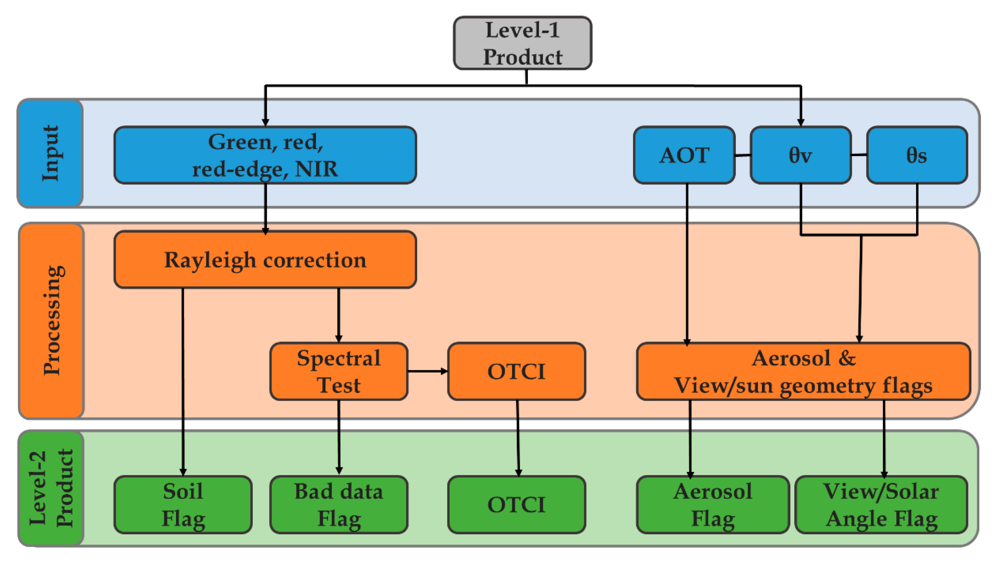
2. Description of the OTCI Product

The Level-2 (L2) OLCI land product Terrestrial Chlorophyll Index (OTCI) that provides continuity to the Envisat MTCI is freely available to the public through the Copernicus Open Access Hub (https://scihub.copernicus.eu/). The Sentinel-3 OTCI is produced at full resolution (300 m) and reduced resolution (1200 m), and is computed from OLCI red, red-edge and NIR bands (Bands 10, 11, and 12) using Equation (1).

$$\mathrm{OTCI}=\frac{\mathrm{Band}12-\mathrm{Band}11}{\mathrm{Band}11-\mathrm{Band}10}=\frac{{\rho }_{753.75}-{\rho }_{708.75}}{{\rho }_{708.75}-{\rho }_{681.25}}$$

(1)

where Band 10, Band 11, Band 12 are the OLCI sensor reflectance bands centred at 681.25, 708.75, 753.75 nm. Similarly, the MTCI is computed using Equation (2).

$$\mathrm{MTCI}=\frac{\mathrm{Band}10-\mathrm{Band}9}{\mathrm{Band}9-\mathrm{Band}8}=\frac{{\rho }_{753.75}-{\rho }_{708.75}}{{\rho }_{708.75}-{\rho }_{681.25}}$$

(2)

where Band 8, Band 9, Band 10 are the MERIS sensor reflectance bands centred at 681.25, 708.75, 753.75 nm. The signal-to-noise ratio (SNR) in OLCI bands is improved by a factor of 2 compared to MERIS bands [52,53] (

Table 1. Sentinel-3 OLCI and Envisat MERIS spectral band signal-to-noise ratio (SNR)

Band Centre	OLCI SNR	MERIS SNR
681.25	1048	485
708.75	1148	531
753.75	861	373

).

The outilne of the Sentinel-3 OTCI algorithm is shown in Figure 1, while the Sentinel-3 OLCI spectral bands and the comparison to Envisat MERIS spectral bands are shown in Figure 2. At present, surface reflectance products are not available directly from OLCI, although it is worth noting third-party atmospheric correction algorithms suitable for OLCI data are now available (e.g., De Keukelaere et al. [54]). Consistent with MERIS, in the operational processing chain, partial atmospheric correction is carried out prior to calculation of the OTCI. First, top of atmosphere (TOA) reflectance is computed from L1B TOA radiance using the solar spectral irradiance and the sun zenith angle [55]. In the next step, gaseous correction is performed to remove the effect of O₃, O₂, and H₂O absorption [56]. Using a separate subroutine, Rayleigh correction is applied to TOA reflectance to account for the effect of molecular scattering [57]. Then, the across track field of view gradient caused by the variation in central wavelength (‘smile effect’) is corrected. An initial spectral test is carried out on land pixels using the NIR band to identify non-vegetated pixels. OTCI is then computed only on the pixels that passed the spectral test. Finally, the quality flags described in the next section are developed.

Uncertainties in land products affect their reliability and fitness for purpose. A key improvement over the Envisat MTCI is the per-pixel uncertainties estimate that is provided with the Sentinel-3 OTCI which are in turn computed from the TOA radiance uncertainties. This is, within the Sentinel-3 OTCI product, uncertainties of the input data are propagated through the algorithm according to the law of propagation of uncertainties as described by Miura [58]. This way, the product has a measure of uncertainty associated to each pixel.

Quality Flags

Documentation of traceable pixel-level quality information is a fundamental principle of the Quality Assurance Framework for Earth Observation [59]. The Sentinel-3 OTCI is accompanied by a data layer with 8-bit encoded information related to individual aspects of data quality: (i) bad data, (ii) view angle, (iii) aerosols, and (iv) soil. The sensitivity analyses and error assessments described below were carried out in the algorithm development and are addressed in more detail in the Sentinel-3 OTCI Algorithm Theoretical Basis Document (ATBD) [60].

The Sentinel-3 OTCI bad data flag consists of spectral tests conducted on pixels classified as land, followed by a range check. The spectral tests, performed on normalised surface reflectance OLCI bands are: (1) band 10 (red) < 0.2, (2) band 12 (NIR) > 0.1, and (3) the difference between band 12 and 10 must be greater than 0.1. Once the three conditions are met, pixel values are verified to fall within the Sentinel-3OTCI expected range (≥0.0 and ≤6.5). Passing the spectral tests and the verification indicates no presence of highly reflective pixels (possibly due to cloud and snow and good data quality). On the contrary, failing the tests indicates presence of clouds or poor data quality. A difference between Envisat MTCI and Sentinel-3 OTCI is the range of acceptable pixel values; empirical evidence suggested that Envisat MTCI maximum value could be increased from 5.5 to 6.5 without risk of saturation.

A viewing and illumination quality flag was developed as follows. First, geometry effects on the L2 product were modelled over a variety of Sun and viewing geometries. Per pixel total uncertainty was modelled for the full OLCI view angle for combinations of solar zenith angle (SZA), solar azimuth angle (SAA), and Sentinel-3 OTCI values. The experiment revealed that the combination of SZA and SAA that resulted in maximum and minimum variation were SZA = 38; SAA = 158 and SZA = 23; SAA = 100, respectively. For a given configuration of SZA and SAA, total variation increases with increase in Sentinel-3 OTCI value. Then, to derive angular ranges for the acquisition and illumination geometry flag, pre-computed uncertainty values for each pixel were stored in a look-up-table (LUT). The LUT contained maximum uncertainty estimations for discrete classes of SZA and view zenith angle (VZA) as a function of predefined Sentinel-3 OTCI ranges. For a given pixel, the following auxiliary data is needed to query the pixel’s uncertainty from the LUT: OTCI, SZA, SAA, and VZA. Example values of the view angle flag are presented in

Table 2. Sentinel-3 OTCI quality flags description for bad data, view angle, aerosol, and soil

Bit	Indicator	Value		Quality	Description
8–7	Bad data	1	1	Very good	ρred < 0.2; ρNIR > 0.1; (ρNIR-ρred) > 0.1
		0	0	Poor	ρred > 0.2; ρNIR < 0.1; (ρNIR-ρred) < 0.1
6–5	View angle	1	1	Very good	VZA < 30°; SZA > 40°
		1	0	Good	VZA 30°< 40°; SZA > 30° ≤ 40°
		0	1	Fair	VZA ≥ 40° < 50°; SZA > 20° ≤ 30°
		0	0	Poor	VZA ≥ 50°; SZA ≤ 20⁰
4–3	Aerosol	1	1	Very good	AOT440 < 0.3
		1	0	Good	AOT440 0.3–0.7
		0	1	Fair	AOT440 0.7–1.4
		0	0	Poor	AOT440 > 1.4
2–1	Soil	1	1	Very good	≥0.9 Land cover non-soil
		1	0	Good	≥0.9 Land cover non-soil
		0	1	Fair	<0.9 Land cover soil
		0	0	Poor	<0.9 Land cover soil

. This was the workflow to establish the angular ranges for the quality flag but this is not implemented in the processor itself.

The scattering in the red region of the spectrum caused by aerosols translates into an increase in the OLCI red band reflectance. Due to its proximity, aerosols have similar effect on the red edge. On the contrary, a decrease in the NIR band is observed due to aerosols absorption in the NIR region. These responses cause a variation of Sentinel-3 OTCI of ~3% at AOT₄₄₀ < 0.3, and up to 21.6% at AOT₄₄₀ > 1.4 [60]. To date, there are no operational AOT estimates available from OLCI (though there is an OLCI and Sea and Land Surface Temperature Radiometer (SLSTR) Synergy AOT product). When AOT information becomes available from OLCI, the flags presented in Table 2 will be implemented. At the time of this paper, these are set as very good condition.

Pixels with bare soil can have Sentinel-3 OTCI values between 1.5 and 1.9 that realistically do not correspond to any CCC. Soil contribution is evaluated using the soil discrimination index (SDI) algorithm (Equation (3)). The SDI, which uses the spectral features of the green, red, and NIR bands, is a combination of the simple ratio index (SR) [61] and the green difference index (GD). The SR is positively correlated to vegetation density whereas the GD is negatively correlated to chlorophyll content with values >3 corresponding to bright bare soils. Establishing an SDI threshold that distinguishes between Sentinel-3 OTCI values <2 due to soil and Sentinel-3 OTCI <2 due to sparse vegetation is necessary. Tests revealed that SDI threshold of 0.9 effectively identifies soil pixels while maintaining vegetated pixels [60].

$$\mathrm{SDI}=\frac{{\rho }_{\mathrm{NIR}}{\rho }_{\mathrm{Red}}}{{\rho }_{\mathrm{Red}}{\rho }_{\mathrm{Green}}}$$

(3)

3. Methods

The consistency of the Sentinel-3 OTCI and Envisat MTCI was evaluated at two distinct scales. Firstly, agreement between the Sentinel-3 OTCI and the Envisat MTCI archive was assessed over specific validation sites, enabling the temporal consistency of the two products to be investigated. Secondly, monthly Sentinel-3 OTCI composites were compared with a monthly Envisat MTCI climatology for the entire globe, enabling the consistency of spatial patterns to be assessed, and facilitating examination by latitude and land cover. In all cases, the comparisons were conducted against the full-mission Envisat MTCI climatology (2002–2012).

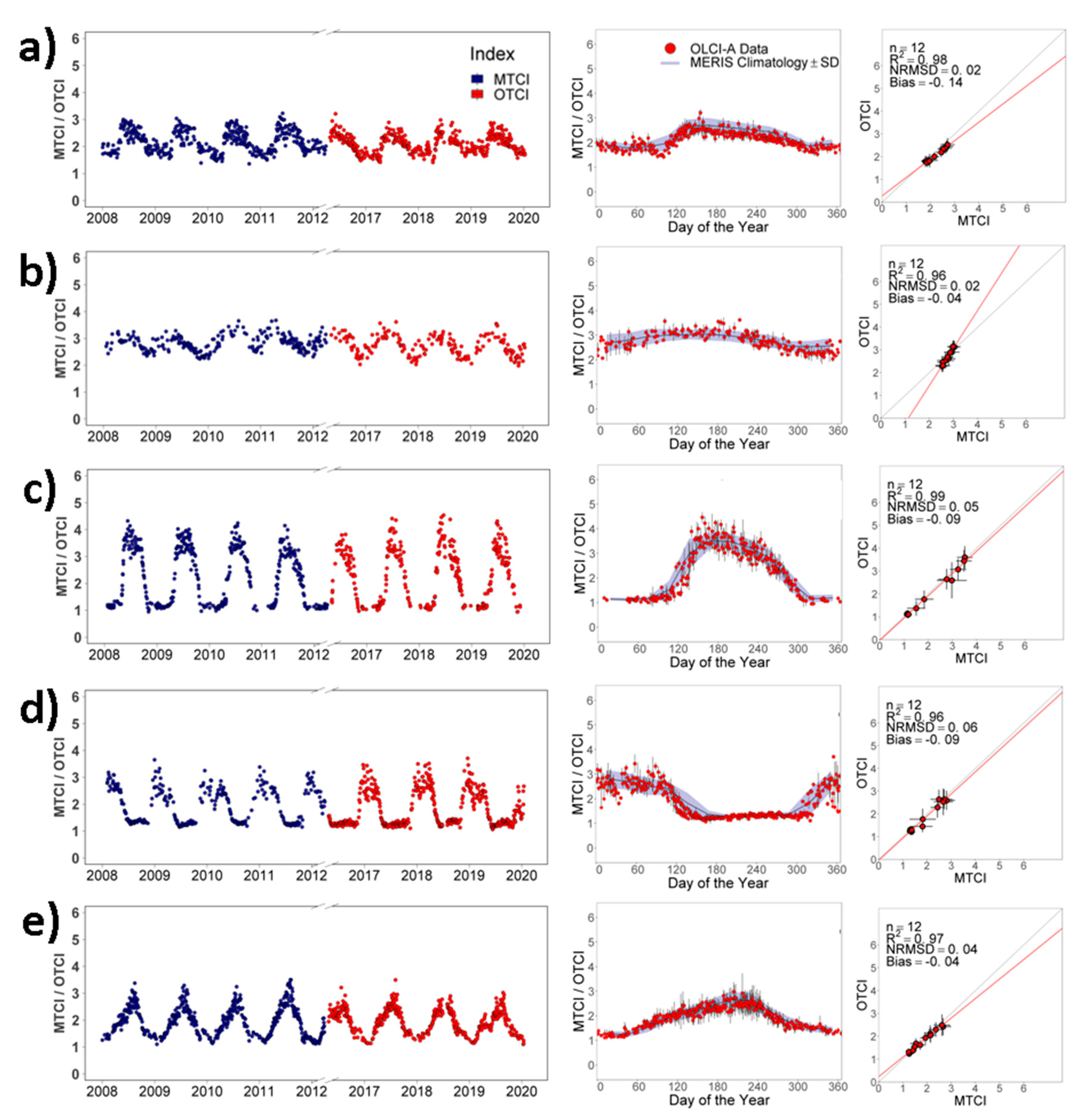
3.1. Evaluating Temporal Consistency at Specific Validation Sites

To assess the temporal consistency of Sentinel-3 OTCI and Envisat MTCI values over specific validation sites, pixel extractions were obtained from Level-2 Sentinel-3 OTCI and third reprocessing (3RP) Envisat MTCI data over 37 validation sites, representing a variety of land cover types, regions, and species (Table S1). The selection of sites included the CEOS WGCV LPV sub-group supersites, which were adopted on the basis of a series of requirements for the validation of land products, and was supplemented by several ‘core’ sites identified by the Sentinel-3 Validation Team (S3VT). The sites are well characterised in terms of canopy structure and biophysical variables, and have long-term monitoring operations with established protocols. The extractions covered a footprint of 3 × 3 full resolution (300 m) pixels to compensate for geometric inaccuracy and the point spread function of the sensors.

3.2. Evaluating Spatial Consistency at the Global Scale

To assess the spatial consistency of Sentinel-3 OTCI and Envisat MTCI values over the entire globe, monthly Level-3 Sentinel-3 OTCI composites were generated using the Sentinel Application Platform (SNAP) binning tool at a 4.6 km spatial resolution. All available Level-2 reduced resolution (RR) products were used as an input. Pixels were filtered according to a Land Quality Science Flag (LQSF) expression that removes clouds, snow, ice, and pixels with out of range Sentinel-3 OTCI inputs/outputs, allowing only the highest quality pixels. The specific LQSF values considered invalid were: LQSF.CLOUD, LQSF.CLOUD_AMBIGUOUS, LQSF.CLOUD_MARGIN, LQSF.SNOW_ICE, and LQSF.OTCI_FAIL. Valid pixels were aggregated using mean value downsampling and mapped to a fixed grid.

For comparison with the monthly Level-3 Sentinel-3 OTCI composites, monthly Level-3 4.6 km Envisat MTCI composites were obtained from the UK Centre for Environmental Data Analysis (CEDA) [62,63]. In this case, the flags used to screen poor quality Envisat MTCI values were: L2_FLAGS.CLOUD, L2_FLAGS.WATER, and LS_FLAGS.PCD_17. Note L2_FLAGS.PCD_17 is a product confidence flag raised if the algorithm input or output falls beyond a valid range (

Table 3. Quality flags applied to exclude unreliable pixels used in the generation of the Envisat MTCI and Sentinel-3 OTCI monthly composites

Product	Quality Flag	Description
	LQSF.CLOUD	Indicates cloudy pixel.
	LQSF.CLOUD_AMBIGUOUS	Possibility of cloudy pixel.
OTCI	LQSF.CLOUD_MARGIN	A margin of 2 pixels around pixels identified as CLOUD & CLOUD_AMBIGUOUS.
	LQSF.SNOW_ICE	Potential presence of ice or snow.
	LQSF.OTCI_FAIL	Denotes that OTCI inputs or outputs are out of range or that Rayleigh correction failed.
	L2_FLAGS.CLOUD	Pixel classification algorithm retrieved a cloudy pixel.
MTCI	L2_FLAGS.WATER	Raised when inland water is detected.
	LS_FLAGS.PCD_17	Atmospheric correction failed or that MTCI inputs or outputs are outside the expected range.

). Once obtained, the mean Envisat MTCI value for each month over all years (2002 to 2012) was computed.

Version 2.0 of the Copernicus Global Land Service Land Cover (CGLS_LC_100) product [64] was used to evaluate global consistency per land cover type. The CGLS_LC_100 is based on PROBA-V time-series (2015 as reference year), a database of land cover training sites, and other ancillary data. The land cover product is mapped to the Sentinel-2 tiling grid and consists of 23 discrete classes at 100 m spatial resolution. The Level-1 map, which is formed by broad cover classes (i.e., bare/sparse vegetation, snow/ice, and permanent water) has an overall accuracy is 80.2 +/−0.7%. The map where closed and open forests are separated (Level-2), has an overall accuracy of 75.1 +/−0.7% [60]. The CGLS_LC_100 product was resampled to match the 4.6 km spatial resolution of the monthly Level-3 OTCI/MTCI composites, using majority (modal) aggregation.

3.3. Statistical Analysis

To quantify agreement between the both products, descriptive statistics, the bias, the coefficient of determination, and the normalised root mean square difference (NRMSD) were used. Comparisons were conducted taking the Envisat MTCI archive as the reference. The bias represents the average difference between the Sentinel-3 OTCI and Envisat MTCI. The sign of the bias is interpreted as over (positive sign) or under (negative sign) estimation. Ideally, the bias should be close to zero. The coefficient of determination (R²) is a measure of the linear relationship between the compared products. The root mean square error (RMSE) is a common statistical indicator of accuracy. However, RMSE is scale dependent and thus specific to a particular variable. The normalisation of the RMSE by the mean (i.e., NRMSD) allows the accuracy of Sentinel-3 OTCI to be compared between other datasets and land products.

4. Results

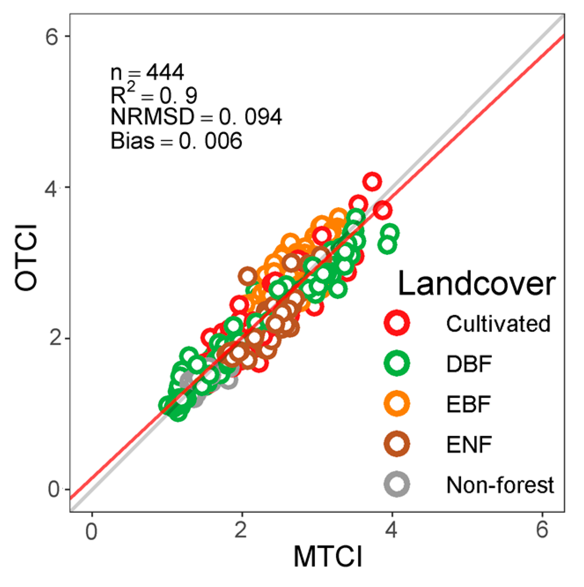
4.1. Temporal Consistency at Specific Validation Sites

Figure 3 shows seasonal trends and scatterplots of the monthly mean for the period 2008 to 2012 (MTCI) and 2016 to 2019 (OTCI) at five sites: US-Talledaga (ENF), AU-Robson-Creek (EBF), FR-Montiers (DBF), BR-Mataseca (non-forest), and IT-Lison (cultivated). Despite the difference in the time period, both Sentinel-3 OTCI and Envisat MTCI temporal profiles exhibit good agreement in the observed seasonal trajectories. Across sites, the profiles are consistent in amplitude and temporal fluctuation, with periods of maximum and minimum activity occurring around the same time every year. At the deciduous forest of FR-Montiers for instance, Envisat MTCI and Sentinel-3 OTCI consistently have maximum values between 3.5 and 4.5 between day of the year (DOY) 150 to 180 (June–July). Similarly, the cultivated site IT-Lison has maximum Envisat MTCI and Sentinel-3 OTCI values of 2.5 to 3.5 between DOY 200 to 230 (mid-July to mid-August). When individual observations were inspected, Sentinel-3 OTCI acquisitions depict a small amount of dispersion, but realistically capture the annual trend of the Envisat MTCI climatology in both hemispheres (middle panel in Figure 3). The comparison of monthly mean values shows moderate to strong agreement (R² = 0.55 to 0.99), low bias (−0.36 to 0.40), and low NRMSD (0.02 to 0.12) (Figure 3 and

Table 4. Statistics of the comparison between monthly mean Sentinel-3 OTCI (2016 to 2019) and Envisat MTCI (2002 to 2012) values over the considered validation sites. Sites are sorted by the NRMSD.

No	Site Acronym	Land Cover	Lat	Lon	MTCI vs. OTCI
					n	R2	NRMSD	Bias
1	AU-Cumberland	EBF	−33.62	150.72	12	0.91	0.02	0
2	AU-Great-Western	DBF	−30.19	120.65	12	0.96	0.02	0.12
3	AU-Litchfield	EBF	−13.18	130.79	12	0.92	0.02	−0.01
4	AU-Robson-Creek	EBF	−17.12	145.63	12	0.96	0.02	−0.04
5	IT-Tra	Cultivated	37.65	12.87	12	0.74	0.02	−0.07
6	SP-Ali	Cultivated	38.45	−1.07	12	0.94	0.02	0.06
7	US-Moab-Site	Non-forest	38.25	−109.39	12	0.56	0.02	0.05
8	US-Talladega	ENF	32.95	−87.39	12	0.98	0.02	−0.14
9	AU-Wombat	EBF	−37.42	144.09	12	0.91	0.03	0.2
10	FR-Guayaflux	EBF	5.28	−52.93	12	0.73	0.03	−0.18
11	FR-Hesse	DBF	48.67	7.07	12	0.99	0.03	0.01
12	US-Harvard	DBF	42.54	−72.17	12	0.99	0.03	−0.12
13	US-Mountain-Lake	DBF	37.38	−80.53	12	0.99	0.03	−0.22
14	AU-Calperum	Non-forest	−34.00	140.59	12	0.46	0.04	0.1
15	AU-Cape-Tribulation	EBF	−16.11	145.38	12	0.86	0.04	−0.06
16	AU-Rushworth	DBF	−36.75	144.97	12	0.84	0.04	0.22
17	AU-Tumbarumba	EBF	−35.66	148.15	12	0.91	0.04	0.4
18	FR-Puechabon	ENF	43.74	3.60	12	0.76	0.04	−0.07
19	IT-Cat	Cultivated	37.28	14.88	12	0.61	0.04	−0.36
20	IT-Lison	Cultivated	45.74	12.75	12	0.97	0.04	−0.04
21	US-Central-Plains	Non-forest	40.82	−104.75	12	0.69	0.04	−0.07
22	US-Oak-Rige	DBF	35.96	−84.28	12	0.99	0.04	−0.04
23	AU-Watts-Creek	EBF	−37.69	145.69	12	0.7	0.05	0.12
24	CR-Santa-Rosa	EBF	10.84	−85.62	12	0.97	0.05	0.16
25	FR-Montiers	DBF	48.54	5.31	12	0.99	0.05	−0.09
26	UK-Wytham-Woods	DBF	51.77	−1.34	12	0.97	0.05	0.08
27	US-Bartlett	DBF	44.06	−71.29	12	0.94	0.05	−0.03
28	AU-Warra-Tall	EBF	−43.10	146.65	12	0.7	0.06	−0.03
29	BR-Mata-Seca	Non-forest	−14.88	−43.97	12	0.96	0.06	−0.09
30	IT-Collelongo	DBF	41.85	13.59	12	0.98	0.06	−0.01
31	SE-Dahra	Cultivated	15.40	−15.43	12	0.6	0.06	−0.04
32	AU-Zigzag-Creek	EBF	−37.47	148.34	12	0.63	0.07	0.3
33	FR-Estrees-Mons	Cultivated	49.87	3.02	12	0.94	0.08	0.06
34	DE-Selhausen	Cultivated	50.87	6.45	12	0.87	0.09	−0.01
35	NE-Loobos	ENF	52.17	5.74	12	0.55	0.09	0.07
36	DE-Geb	Cultivated	51.10	10.91	12	0.89	0.1	−0.1
37	FR-Aurade	Cultivated	43.55	1.11	12	0.78	0.12	0.09

).

Figure 4 presents the monthly mean of all 37 sites for the entire archive of both products (12 years for Envisat MTCI and 4 years of Sentinel-3 OTCI). There is very strong agreement between both products (R² = 0.9; NRMSD < 0.10). There is more dispersion towards higher values; the Sentinel-3 OTCI shows minimal underestimation for DBF in values >3, whereas EBF depicts slight overestimation. In general, however, the observed bias is marginal (0.006).

4.2. Spatial Consistency at the Global Scale

This section compares Envisat MTCI and Sentinel-3 OTCI global composites. Northern hemisphere winter (summer in the southern hemisphere) and summer (winter in the southern hemisphere), periods were investigated as they correspond to times of contrasting vegetation photosynthetic activity. Overall, both products realistically capture the spatial patterns of CCC. Key findings are described below.

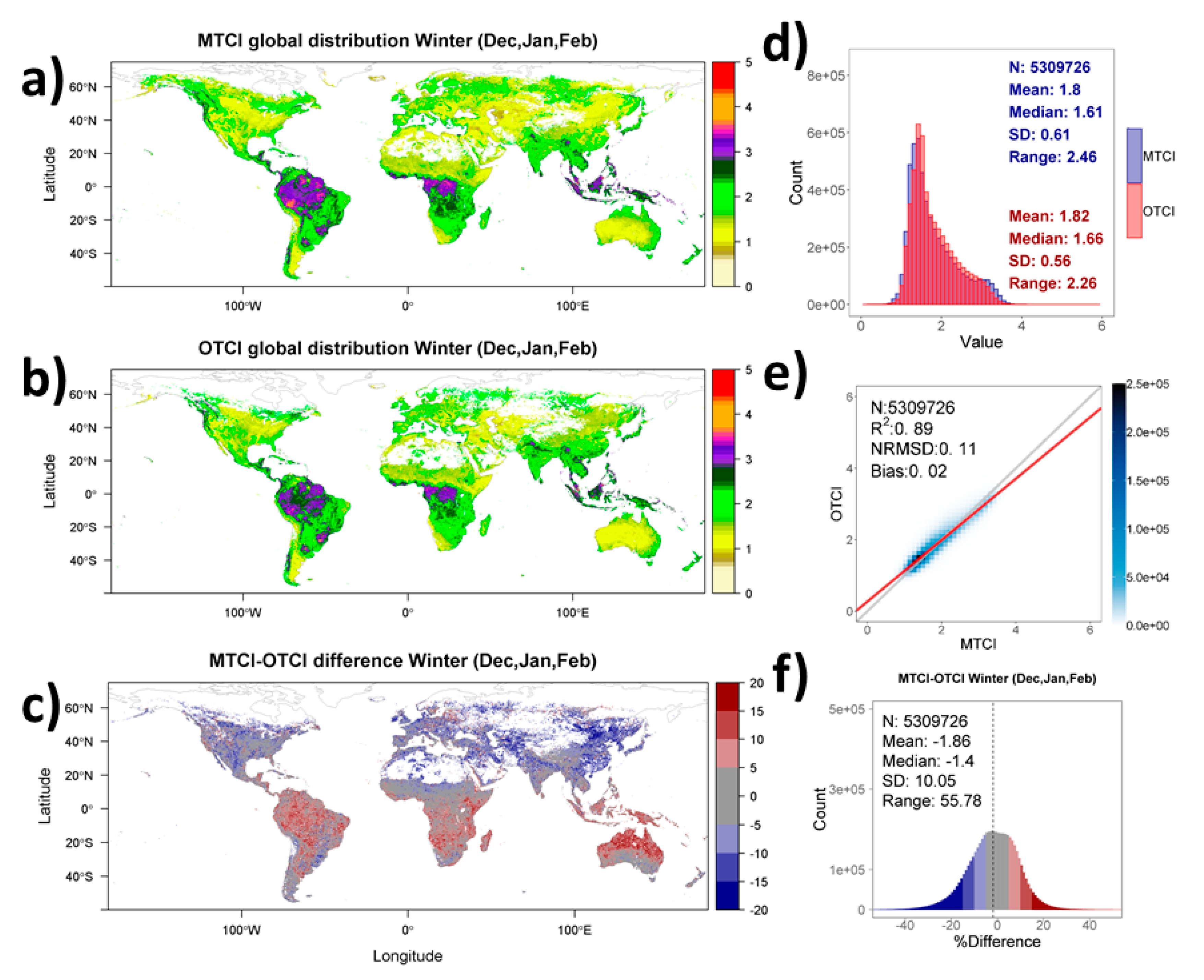
4.2.1. Northern Hemisphere Winter (Dec, Jan, Feb)

Figure 5a,b show the spatial distribution of Envisat MTCI and Sentinel-3 OTCI values for the northern hemisphere winter season (Dec, Jan, Feb). Both products depict a similar spatial pattern characterised by comparatively higher values in the Amazon and Congo basins, north Indian subcontinent, and South East Asia. Lower vegetation activity is observed in Northern and Central America, Northern and Horn of Africa, Europe, Russia, and central and west of Australia. Data gaps are evident in the Sahara desert, Arabian Peninsula, and Gobi desert. Due to cloudiness, snow cover, and low sun angle, data gaps occur at higher latitudes above 65°.

In both products, the frequency distribution of pixel values is skewed to the left (i.e., indicating a higher concentration of lower values) and bimodal, dominated by a high peak around 1.5 and a small peak around 3. The mean of the Sentinel-3 OTCI (1.82) is slightly larger than the Envisat MTCI (1.80), whilst the dispersion is greater in MTCI (standard deviation = 0.61; range = 2.46) compared to Sentinel-3 OTCI (standard deviation = 0.56; range = 2.26).

The scatterplot indicates good agreement between the products in winter, showing a linear fit close to the 1:1 line (R² = 0.89). The statistical metrics depicts low error (NRMSD = 0.11) but slight overestimation when compared to the Envisat MTCI (bias = 0.02). The percentage difference histogram is unimodal it has a flattened nearly symmetrical shape. The mean percentage difference is −1.86 (10.05% standard deviation) and the range between 5th and 95th percentile is 55.78%. In addition, 67% of land mass has a difference less than 10%.

Figure 5c shows the gridded spatial variability of MTCI-OTCI difference for winter. Major negative differences (in blue), where the Sentinel-3 OTCI is greater than the Envisat MTCI, occur in East and South Central China, the Indo-Gangetic Plain, the southern portion of European Russia, Europe, and the east of South America (predominately agricultural region). Most of the positive differences (in red, where the Envisat MTCI is greater than the Sentinel-3 OTCI, occur in the Amazon and Congo basins, the north of Eastern Europe, the north of Australia, and South East Asia.

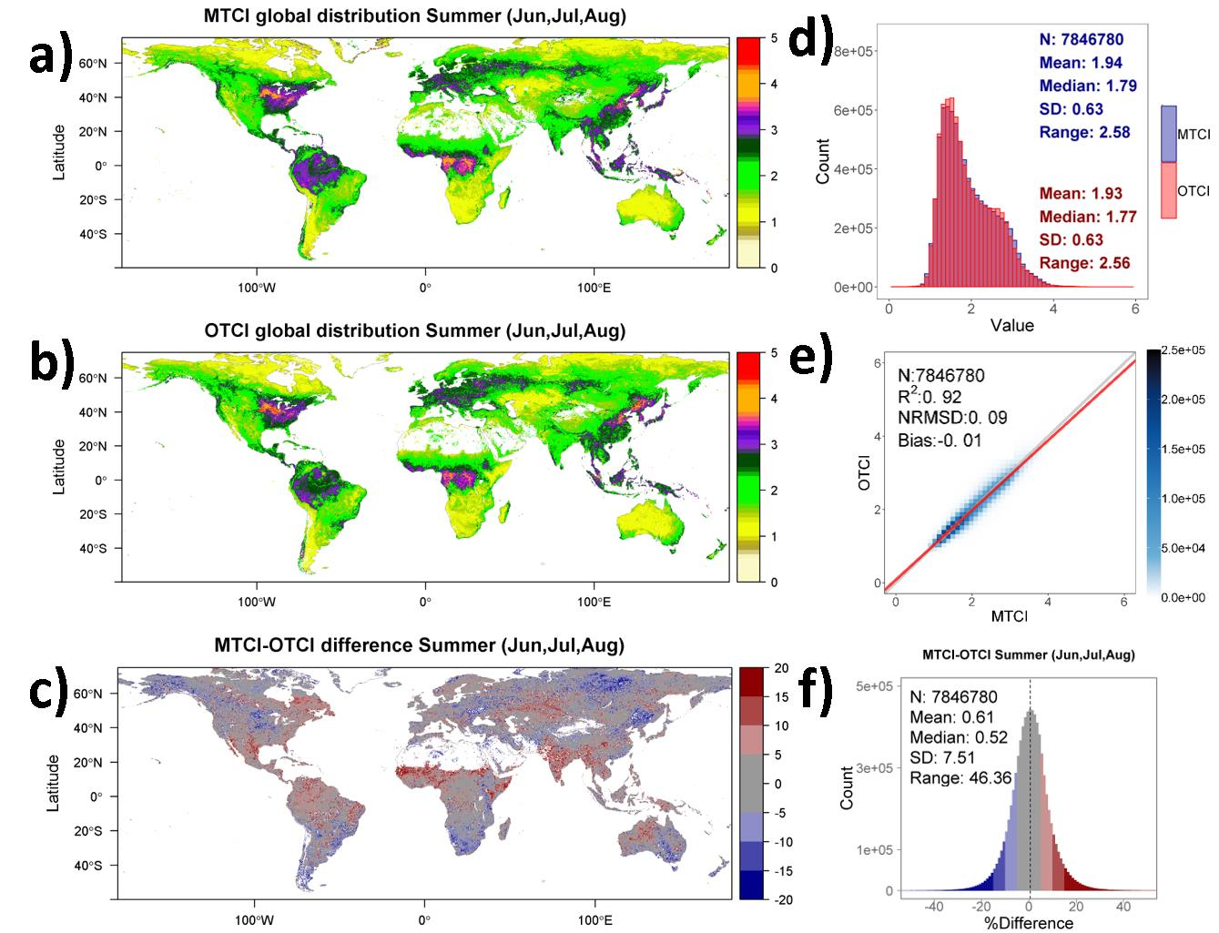
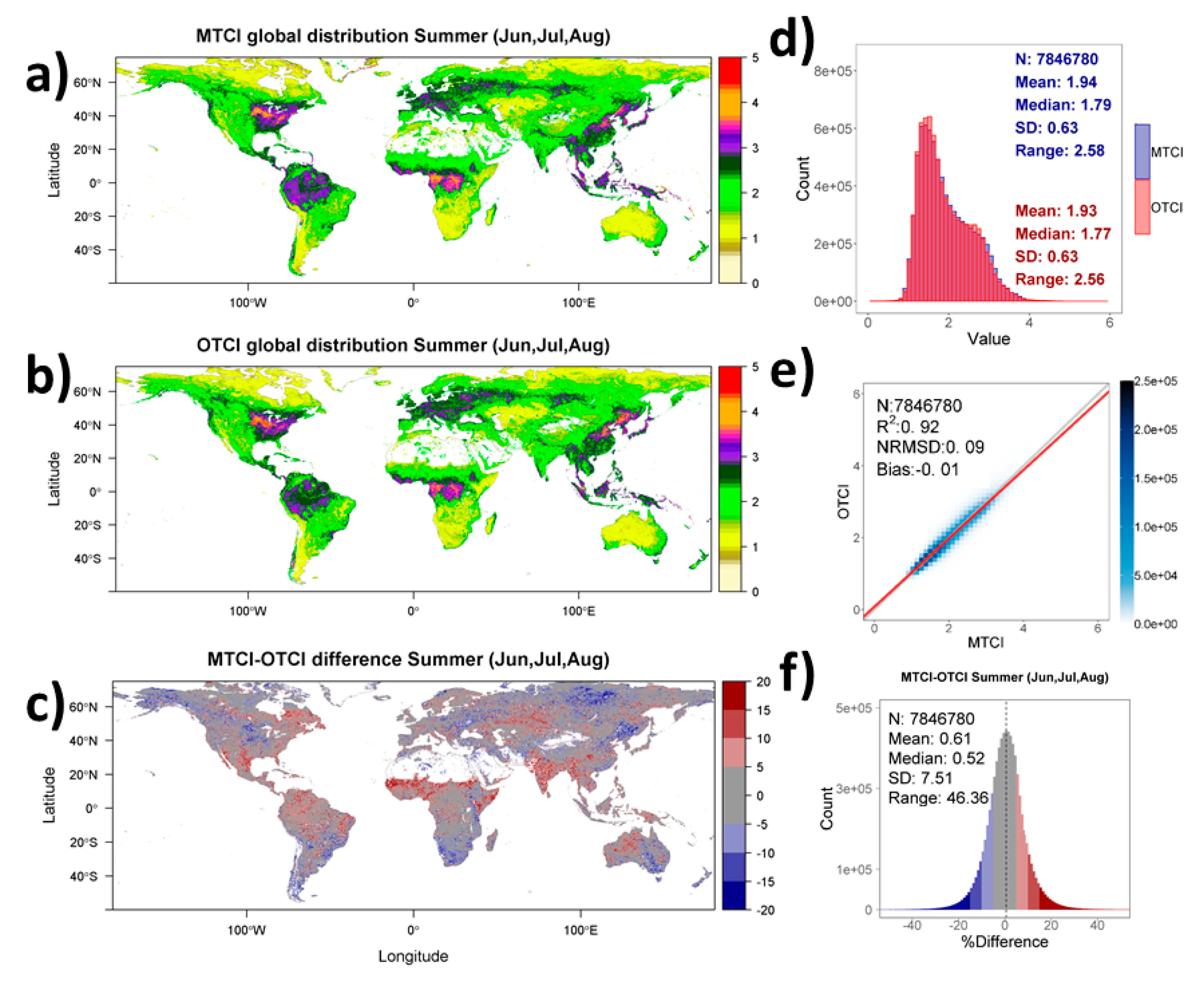
4.2.2. Northern Hemisphere Summer (Jun, Jul, Aug)

The spatial pattern of the Envisat MTCI and Sentinel-3 OTCI for summer (Jun, Jul, Aug) is shown in Figure 6a,b. The products reflect higher vegetation activity in the northern hemisphere and depict strong spatial agreement. Maximum values are observed in east of the United States, the Amazon and Congo rainforests, Europe and European Russia, the north of India, the east of China, and South East Asia. Areas of lower vegetation activity are the world’s tundra (the north of Canada and Russia) and the herbaceous landscapes of Kazakhstan, South America, the south and horn of Africa, and central and west of Australia. Summer maps have substantially less missing data when compared to winter.

With respect to the frequency distribution of values, like the winter, Figure 6d shows the histograms are skewed to the left and bimodal. A dominant peak of values is located between 1.5 and 2.0, and a second smaller peak is located between 2.0 and 3.0. Overall, the mean and spread is marginally greater for Envisat MTCI (mean = 1.94; standard deviation = 0.63; range = 2.58) than for Sentinel-3 OTCI (mean = 1.93; standard deviation = 0.77; range = 2.56).

The scatterplot further reflects the strong agreement. Quantitatively, the 1:1 comparison showed R² = 0.92, NRMSD = 0.09, and absolute bias = 0.01. Geographically, discrepancies where the Sentinel-3 OTCI is higher than the Envisat MTCI (blue) are located in the Midwest United States, Ukraine, and Northeast China (dominated agricultural land). On the contrary, areas where the Envisat MTCI is higher than the Sentinel-3 OTCI (red a), are found in the west United States and Mexico, the Amazon rainforest, west Africa, and southern Asia. The frequency distribution of percentage differences is symmetrical and unimodal with a mean and median of 0.61% (7.51 standard deviation), the range between the 5th and 95th percentile is 46.36%. Finally, the percentage of land mass with less than 10% is 81%.

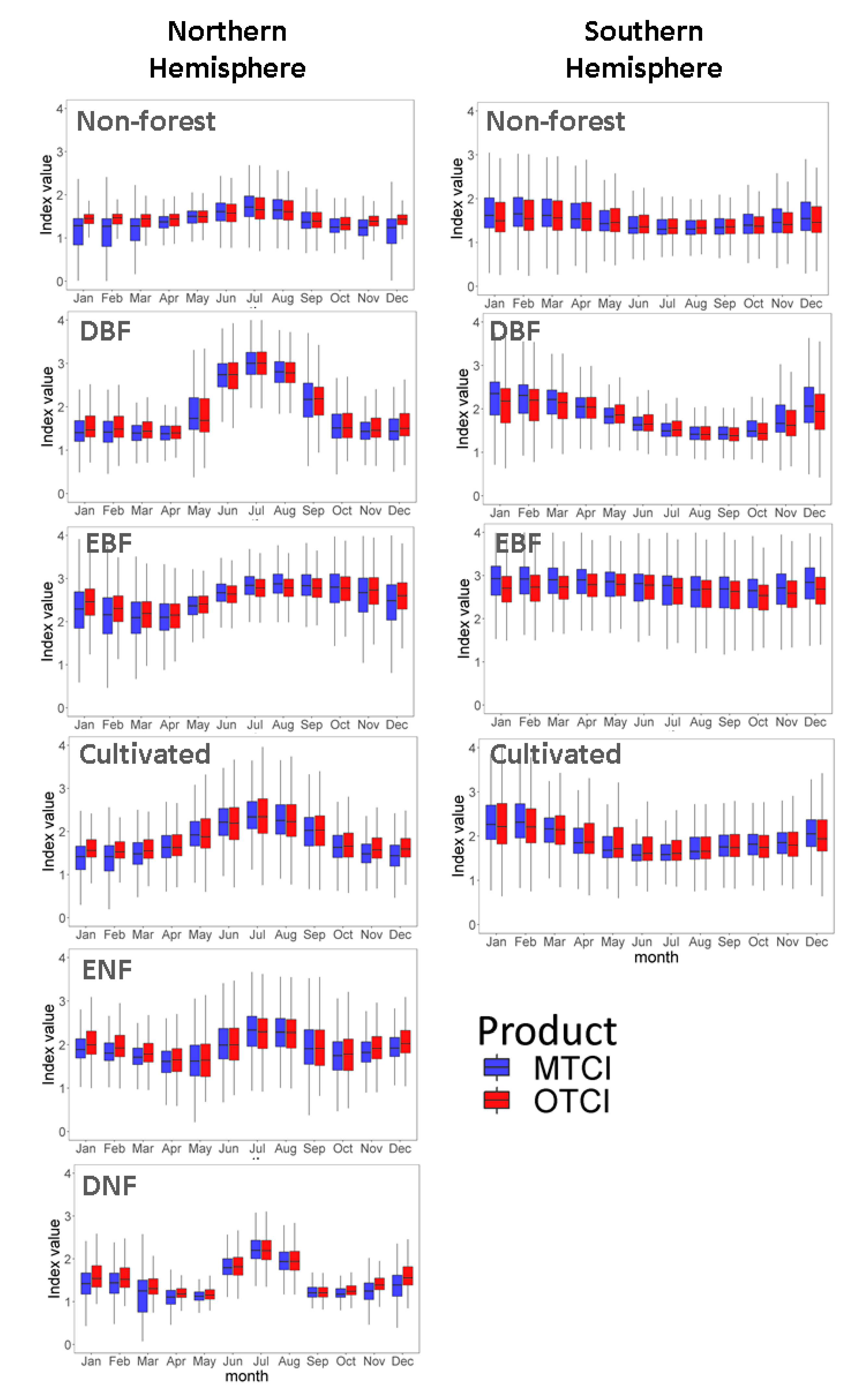
4.2.3. Latitudinal Variation

Latitudinal variation data comparison has been presented in Figure 7.

Figure 7 compares the mean (±1 standard deviation) latitudinal gradient of the products over four seasons. Maximum values (>2.5) are found at the tropics (±10°), whereas minimum values at higher latitudes (>50° north and >30° south). In the region of maximum vegetation activity (±10°), the Envisat MTCI remains marginally higher than the Sentinel-3 OTCI. However, overall the products exhibit high correlation (R² > 0.96), with no apparent bias. The products exhibit latitudinal seasonal variations. For instance, in summer a peak emerges at 20° latitude that persists until autumn, and dispersion increases between 30° and 45°.

4.2.4. Consistency by Land Cover

Statistical results of product comparisons for six land cover classes (ENF, EBF, DNF, DBF, non-forest, and cultivated) across four seasons is presented in

Table 5. Summary statistics per land cover: evergreen needleleaf (ENF), evergreen broadleaf (EBF), deciduous needleleaf (DNF), deciduous broadleaf (DBF), non-forest, and cultivated

Hemisphere	Cover	Winter Dec, Jan, Feb				Spring Mar, Apr, May				Summer Jun, Jul, Aug				Autumn Sep, Oct, Nov
		N	R2	NRMSD	Bias	N	R2	NRMSD	Bias	N	R2	NRMSD	Bias	N	R2	NRMSD	Bias
	ENF	188,711	0.66	0.10	0.10	280,023	0.89	0.09	−0.03	281,429	0.91	0.07	−0.06	281,443	0.91	0.08	0.01
	EBF	159,333	0.78	0.08	0.05	159,295	0.81	0.07	−0.03	159,242	0.72	0.06	−0.10	159,357	0.72	0.07	−0.05
Northern	DNF	60,637	0.69	0.13	0.10	152,654	0.69	0.08	0.00	152,682	0.76	0.07	0.00	152,681	0.71	0.08	0.01
	DBF	310,958	0.75	0.11	0.09	378,122	0.85	0.07	0.01	379,087	0.71	0.07	−0.01	379,095	0.89	0.07	0.02
	Non-forest	799,813	0.71	0.09	0.08	1,124,841	0.81	0.08	0.01	1,155,969	0.85	0.08	−0.05	1,156,648	0.87	0.06	0.02
	Cultivated	797,428	0.74	0.12	0.12	919,764	0.83	0.10	0.04	920,133	0.83	0.10	0.00	920,388	0.82	0.09	0.05
	EBF	243,118	0.81	0.06	−0.18	243,146	0.71	0.07	−0.08	242,667	0.77	0.08	−0.03	243,159	0.84	0.06	−0.11
Southern	DBF	169,079	0.94	0.05	−0.14	169,079	0.88	0.06	−0.02	168,556	0.83	0.07	0.02	169,078	0.88	0.07	−0.06
	Non-forest	708,946	0.90	0.08	−0.09	709,024	0.88	0.09	−0.02	704,668	0.84	0.09	0.01	708,718	0.90	0.07	−0.03
	Cultivated	131,860	0.84	0.11	0.00	131,866	0.74	0.14	0.09	131,862	0.73	0.11	0.05	131,869	0.78	0.08	−0.01

. In general, in the northern hemisphere, the strongest agreement occurred in spring and autumn (R² > 0.87), particularly for ENF and DBF. In the southern hemisphere, the strongest agreement was for winter and autumn in particular for DBF and non-forest (R² > 0.87). In the north, the poorest agreement was for DNF whereas in the south it was for cultivated land. In both hemispheres, the largest NRMSD was observed in the cultivated land. On average, NRMSD remained ≤0.11 across seasons and land cover types. Similarly, bias remained ≤0.10 across seasons except for EBF and DBF in winter in the south. The monthly evolution of the products further depicts their seasonal consistency in Figure 8. Notably, for EBF, DNF, non-forest, and cultivated, the winter and autumn months show a greater discrepancy, where the Envisat MTCI interquartile range is greater and the Sentinel-3 OTCI median is higher, reflecting an overestimation.

5. Discussion

5.1. Product Performance

The results of the temporal and spatial comparison between the Envisat MTCI and Sentinel-3 OTCI revealed strong agreement despite the time gap between the two missions. Globally, both products are strongly correlated (R² ≥ 0.89) with low absolute difference (NRMSD ≤ 0.11) and absolute bias (≤0.02). This agreement is not surprising as OLCI has a similar mechanical and optical design to MERIS (Figure 2), albeit with improvements including higher signal-to-noise ratio (Table 1), increased radiometric stability, shorter revisit times (~2 days). This agreement provides a solid case to use Sentinel-3 OTCI as a continuity of the Envisat MTCI time-series. Thus, potentially building a unique data set of canopy chlorophyll content going back to 2002 (with data gap 2012–2014). Further research on spectral similarity between the MERIS and OLCI sensor and their continuity would strengthen the case.

Notably, the global maps show differences up to 16–20% in some regions such as the Amazon basin, sub-Saharan Africa, and north of Australia. The spatial distribution and the magnitude of discrepancies varied between seasons. For instance, higher agreement is observed in summer (Jun, Jul, Aug) where 81% of the land mass had a difference of less than 10% (Figure 5f and Figure 6f). Discrepancies between the products occurred in agricultural and densely forested areas. Whilst some discrepancies might theoretically be explained by differences in sensor viewing geometry and geolocation, experimental data demo3nstrated the impact of viewing geometry on the computed index values is marginal [60]. Furthermore, in this study, geolocation inaccuracies were minimized by using reduced resolution products. Overpass time could be discarded as a contributing factor as both, Envisat and Sentinel-3 were configured to fly in a sun-synchronous orbit at a local equatorial crossing time of 10:00 a.m. [53]. Differences in land management practices, land conversion and extreme climatic events resulting in productivity fluctuations during the gap between missions could be contributing factors. However, further investigation is necessary to improve our understanding. In the first instance, a detailed analysis of these factors over the validation sites used in this research could be a starting point.

Limitations with this study should be noted. Firstly, the compared datasets are not contemporaneous but there is a gap of four years between them. MERIS ceased operations in 2012 and OLCI was launched in 2016. Generally, intercomparisons are conducted with time-overlapping products. This introduces uncertainties due to interannual variations and extreme events. Furthermore, data available for Envisat MTCI span 10 years (2002–2012) whereas the OTCI archive is 3 years (2016–2019), which makes the Sentinel-3 OTCI more sensitive to outliers. This can be seen in Figure 1 (middle column) where Sentinel-3 OTCI presents abrupt transitions. Nevertheless, in the absence of other operational CCC products, the approach offers useful insights into product performance.

5.2. OTCI Applications and Future Work

The results of this study give confidence to users that the Sentinel-3 OTCI can provide continuity to the established MERIS archive. By taking advantage of guaranteed data availability through the Copernicus programme and leveraging several algorithm improvements, the Sentinel-3 OTCI has the potential for applications in risk management such as livestock and crop insurance, gross primary productivity (GPP) modelling, the investigation of vegetation responses to climate change, and food security.

To ensure continued utility of the Sentinel-3 OTCI, future work should focus on direct validation using traceable in situ measurements of CCC (as is being considered in the Fiducial Reference Measurements for Vegetation (FRM4VEG) project). Another opportunity is the indirect verification of OLCI A/B. Although at the moment Sentinel-3 B mission duration is too short (May 2018–present) to allow robust intercomparisons, eventually, comparisons between S3 units will help establish relative uncertainty characterisations. Initial results suggest there is no difference between A and B units [65], this should continue into the future to investigate any potential impact of sensor degradation on the Sentinel-3 OTCI.

The CEOS LPV and ESA Core validation sites selected in this research include a wide range of latitudes (52N to 43S) and vegetation types. However, these sites are concentrated in the United States, Europe, and Australia. This highlights the need to expand the geographical representativeness. Future work may consider including tropical and higher latitude sites (e.g., tundra) in addition to underrepresented regions such as Central and South America, Africa, and Asia.

Quantitative analysis of between-sensor difference is crucial for long-term climate change studies. Although Sentinel-3 OLCI has similar design as Envisat MERIS with nearly identical spectral bands (Figure 2), contribution of differences in solar-viewing geometry, spectral bandwidth, and spectral response function cannot be entirely ruled out. BRDF corrections and spectral adjustment are ways to remove these effects and harmonise the two products, which could be considered in future work (e.g., Claverie, et al. [66]). Performing these corrections was beyond the scope of this research, because the aim is to assess the consistency between Envisat MTCI and Sentinel-3 OTCI that are currently available to the end user.

An additional area of opportunity to maximise the utility of the Sentinel-3 OTCI is the production and dissemination of Level-3 composites, since spatiotemporal syntheses rather than Level-2 products are required by many downstream applications. Within the Sentinel-3 Mission Performance Centre (S3MPC), production of Level-3 products mapped on a common grid, projection, and spatial extent are planned in the near future.

6. Conclusions

Sentinel-3 has been in operation since April 2016 delivering the OTCI. This product provides continuity to the related land products derived from Envisat MTCI. The Sentinel-3 OTCI has been released to the public, therefore, there is a need to evaluate the product’s spatial and temporal consistency with the Envisat MTCI archive. This paper presents a description of the Sentinel-3 OTCI algorithm and the intercomparison of 3 years (2016–2019) of Sentinel-3 OTCI data against 10 years (2002–2012) of Envisat MTCI data, making use of a MERIS climatology. The strong spatial and temporal consistency between the Sentinel-3 OTCI and Envisat MTCI demonstrated in this study provides confidence to users of the product. Future work will involve direct validation using in situ reference measurements following best practices and protocols, Sentinel-3 A and B unit intercomparisons, and L3 product development.

References

1. Gitelson, A.A.; Peng, Y.; Viña, A.; Arkebauer, T.; Schepers, J.S. Efficiency of chlorophyll in gross primary productivity: A proof of concept and application in crops. J. Plant. Physiol. 2016, 201, 101–110. [Google Scholar] [CrossRef] [Green Version]
2. Croft, H.; Chen, J.M.; Luo, X.; Bartlett, P.; Chen, B.; Staebler, R.M. Leaf chlorophyll content as a proxy for leaf photosynthetic capacity. Glob. Chang. Biol. 2017, 23, 3513–3524. [Google Scholar] [CrossRef]
3. Ogutu, B.O.; Dash, J.; Dawson, T.P. Developing a diagnostic model for estimating terrestrial vegetation gross primary productivity using the photosynthetic quantum yield and Earth Observation data. Glob. Chang. Biol. 2013, 19, 2878–2892. [Google Scholar] [CrossRef] [PubMed]
4. Peng, Y.; Gitelson, A.A. Remote estimation of gross primary productivity in soybean and maize based on total crop chlorophyll content. Remote Sens. Environ. 2012, 117, 440–448. [Google Scholar] [CrossRef]
5. Carter, G.A.; Knapp, A.K. Leaf optical properties in higher plants: Linking spectral characteristics to stress and chlorophyll concentration. Am. J. Bot. 2001, 88, 677–684. [Google Scholar] [CrossRef] [PubMed] [Green Version]
6. Carter, G.A. Ratios of leaf reflectances in narrow wavebands as indicators of plant stress. Int. J. Remote Sens. 1994, 15, 517–520. [Google Scholar] [CrossRef]
7. Sampson, P.H.; Zarco-Tejada, P.J.; Mohammed, G.H.; Miller, J.R.; Noland, T.L. Hyperspectral Remote Sensing of Forest Condition: Estimating Chlorophyll Content in Tolerant Hardwoods. For. Sci. 2003, 49, 381–391. [Google Scholar] [CrossRef]
8. Houlès, V.; Guérif, M.; Mary, B. Elaboration of a nitrogen nutrition indicator for winter wheat based on leaf area index and chlorophyll content for making nitrogen recommendations. Eur. J. Agron. 2007, 27, 1–11. [Google Scholar] [CrossRef]
9. Heege, H.J.; Reusch, S.; Thiessen, E. Prospects and results for optical systems for site-specific on-the-go control of nitrogen-top-dressing in Germany. Precis. Agric. 2008, 9, 115–131. [Google Scholar] [CrossRef]
10. Arnon, D.I. Copper enzymes in isolated chloroplasts. Polyphenoloxidase in beta vulgaris. Plant. Physiol. 1949, 24, 1–15. [Google Scholar] [CrossRef] [Green Version]
11. Lichtenthaler, H.K. Chlorophylls and Carotenoids: Pigments of Photosynthetic Biomembranes. Methods Enzymol. 1987, 148, 350–382. [Google Scholar] [CrossRef]
12. Richardson, A.D.; Duigan, S.P.; Berlyn, G.P. An evaluation of noninvasive methods to estimate foliar chlorophyll content. New Phytol. 2002, 153, 185–194. [Google Scholar] [CrossRef] [Green Version]
13. Cerovic, Z.G.; Masdoumier, G.; Ghozlen, N.B.; Latouche, G. A new optical leaf-clip meter for simultaneous non-destructive assessment of leaf chlorophyll and epidermal flavonoids. Physiol. Plant. 2012, 146, 251–260. [Google Scholar] [CrossRef] [PubMed]
14. Ciganda, V.; Gitelson, A.; Schepers, J. Non-destructive determination of maize leaf and canopy chlorophyll content. J. Plant. Physiol. 2009, 166, 157–167. [Google Scholar] [CrossRef] [PubMed] [Green Version]
15. Botha, E.J.; Leblon, B.; Zebarth, B.; Watmough, J. Non-destructive estimation of potato leaf chlorophyll from canopy hyperspectral reflectance using the inverted PROSAIL model. Int. J. Appl. Earth Obs. Geoinf. 2007, 9, 360–374. [Google Scholar] [CrossRef]
16. Vuolo, F.; Dash, J.; Curran, P.J.; Lajas, D.; Kwiatkowska, E. Methodologies and Uncertainties in the Use of the Terrestrial Chlorophyll Index for the Sentinel-3 Mission. Remote Sens. 2012, 4, 1112–1133. [Google Scholar] [CrossRef] [Green Version]
17. Heenkenda, M.K.; Joyce, K.E.; Maier, S.W.; De Bruin, S. Quantifying mangrove chlorophyll from high spatial resolution imagery. ISPRS J. Photogramm. Remote Sens. 2015, 108, 234–244. [Google Scholar] [CrossRef]
18. Delloye, C.; Weiss, M.; Defourny, P. Retrieval of the canopy chlorophyll content from Sentinel-2 spectral bands to estimate nitrogen uptake in intensive winter wheat cropping systems. Remote Sens. Environ. 2018, 216, 245–261. [Google Scholar] [CrossRef]
19. Dash, J.; Ogutu, B.O. Recent advances in space-borne optical remote sensing systems for monitoring global terrestrial ecosystems. Prog. Phys. Geogr. Earth Environ. 2016, 40, 322–351. [Google Scholar] [CrossRef]
20. Frampton, W.J.; Dash, J.; Watmough, G.; Milton, E.J. Evaluating the capabilities of Sentinel-2 for quantitative estimation of biophysical variables in vegetation. ISPRS J. Photogramm. Remote Sens. 2013, 82, 83–92. [Google Scholar] [CrossRef] [Green Version]
21. Rast, M.; Bézy, J.L.; Bruzzi, S. The ESA Medium Resolution Imaging Spectrometer MERIS a review of the instrument and its mission. Int. J. Remote Sens. 1999, 20, 1681–1702. [Google Scholar] [CrossRef]
22. Curran, P.J.; Steele, C.M. MERIS: The re-branding of an ocean sensor. Int. J. Remote Sens. 2005, 26, 1781–1798. [Google Scholar] [CrossRef]
23. Dash, J.; Curran, P.J. The MERIS terrestrial chlorophyll index. Int. J. Remote Sens. 2004, 25, 5403–5413. [Google Scholar] [CrossRef]
24. Demetriades-Shah, T.H.; Steven, M.D.; Clark, J.A. High resolution derivative spectra in remote sensing. Remote Sens. Environ. 1990, 33, 55–64. [Google Scholar] [CrossRef]
25. Dawson, T.P.; Curran, P.J. Technical note A new technique for interpolating the reflectance red edge position. Int. J. Remote Sens. 1998, 19, 2133–2139. [Google Scholar] [CrossRef]
26. Bonham-Carter, G.F. Numerical procedures and computer program for fitting an inverted gaussian model to vegetation reflectance data. Comput. Geosci. 1988, 14, 339–356. [Google Scholar] [CrossRef]
27. Guyot, G.; Baret, F.; Jacquemoud, S. Imaging spectroscopy for vegetation studies. Imaging Spectrosc. Fundam. Prospect. Appl. 1992, 2, 145–165. [Google Scholar]
28. Fernandes, R.; Plummer, S.E.; Nightingale, J.; Baret, F.; Camacho, F.; Fang, H.; Garrigues, S.; Gobron, N.; Lang, M.; Lacaze, R.; et al. Global Leaf Area Index Product Validation Good Practices. Version 2.0. Best Pract. Satelitte-Derived L. Prod. Valid. L. Prod. Valid. Subgr. 2014, 1–78. [Google Scholar] [CrossRef]
29. Yoder, B.J.; Johnson, L.F. Seedling Canopy Chemistry, 1992–1993 (ACCP); ORNL DAAC: Oak Ridge, TN, USA, 1999. [CrossRef]
30. Dash, J.; Curran, P.J.; Tallis, M.J.; Llewellyn, G.M.; Taylor, G.; Snoeijf, P. Validating the MERIS terrestrial chlorophyll index (MTCI) with ground chlorophyll content data at MERIS spatial resolution. Int. J. Remote Sens. 2010, 31, 5513–5532. [Google Scholar] [CrossRef] [Green Version]
31. Dash, J.; Jeganathan, C.; Atkinson, P.M. The use of MERIS Terrestrial Chlorophyll Index to study spatio-temporal variation in vegetation phenology over India. Remote Sens. Environ. 2010, 114, 1388–1402. [Google Scholar] [CrossRef]
32. Rodriguez-Galiano, V.F.; Dash, J.; Atkinson, P.M. Characterising the land surface phenology of Europe using decadal MERIS data. Remote Sens. 2015, 7, 9390–9409. [Google Scholar] [CrossRef] [Green Version]
33. Boyd, D.S.; Almond, S.; Dash, J.; Curran, P.J.; Hill, R.A. Phenology of vegetation in southern england from envisat meris terrestrial chlorophyll index (MTCI) data. Int. J. Remote Sens. 2011, 32, 8421–8447. [Google Scholar] [CrossRef] [Green Version]
34. Jin, J.; Jiang, H.; Zhang, X.; Wang, Y. Characterizing spatial-temporal variations in vegetation phenology over the north-south transect of northeast asia based upon the MERIS terrestrial chlorophyll index. Terr. Atmos. Ocean. Sci. 2012, 23, 413–424. [Google Scholar] [CrossRef] [Green Version]
35. Jeganathan, C.; Dash, J.; Atkinson, P.M. Mapping the phenology of natural vegetation in India using a remote sensing-derived chlorophyll index. Int. J. Remote Sens. 2010, 31, 5777–5796. [Google Scholar] [CrossRef]
36. Zurita-Milla, R.; Clevers, J.G.P.W.; Van Gijsel, J.A.E.; Schaepman, M.E. Using MERIS fused images for land-cover mapping and vegetation status assessment in heterogeneous landscapes. Int. J. Remote Sens. 2011, 32, 973–991. [Google Scholar] [CrossRef]
37. Dash, J.; Mathur, A.; Foody, G.M.; Curran, P.J.; Chipman, J.W.; Lillesand, T.M. Land cover classification using multi-temporal MERIS vegetation indices. Int. J. Remote Sens. 2007, 28, 1137–1159. [Google Scholar] [CrossRef] [Green Version]
38. Ullah, S.; Si, Y.; Schlerf, M.; Skidmore, A.K.; Shafique, M.; Iqbal, I.A. Estimation of grassland biomass and nitrogen using MERIS data. Int. J. Appl. Earth Obs. Geoinf. 2012, 19, 196–204. [Google Scholar] [CrossRef]
39. Loozen, Y.; Rebel, K.T.; Karssenberg, D.; Wassen, M.J.; Sardans, J.; Peñuelas, J.; De Jong, S.M. Remote sensing of canopy nitrogen at regional scale in Mediterranean forests using the spaceborne MERIS Terrestrial Chlorophyll Index. Biogeosciences 2018, 15, 2723–2742. [Google Scholar] [CrossRef] [Green Version]
40. Zhang, S.; Liu, L. The potential of the MERIS Terrestrial Chlorophyll Index for crop yield prediction. Remote Sens. Lett. 2014, 5, 733–742. [Google Scholar] [CrossRef]
41. Dash, J.; Curran, P.J. Relationship between the MERIS vegetation indices and crop yield for the state of South Dakota, USA. In Proceedings of the European Space Agency, (Special Publication) ESA SP, Montreux, Switzerland, 23–27 April 2007. [Google Scholar]
42. Chiwara, P.; Ogutu, B.O.; Dash, J.; Milton, E.J.; Ardö, J.; Saunders, M.; Nicolini, G. Estimating terrestrial gross primary productivity in water limited ecosystems across Africa using the Southampton Carbon Flux (SCARF) model. Sci. Total Environ. 2018, 630, 1472–1483. [Google Scholar] [CrossRef] [Green Version]
43. Boyd, D.S.; Almond, S.; Dash, J.; Curran, P.J.; Hill, R.A.; Foody, G.M. Evaluation of envisat MERIS terrestrial chlorophyll index-based models for the estimation of terrestrial gross primary productivity. IEEE Geosci. Remote Sens. Lett. 2012, 9, 457–461. [Google Scholar] [CrossRef]
44. Harris, A.; Dash, J. A new approach for estimating northern peatland gross primary productivity using a satellite-sensor-derived chlorophyll index. J. Geophys. Res. 2011, 116. [Google Scholar] [CrossRef] [Green Version]
45. Donlon, C.; Berruti, B.; Buongiorno, A.; Ferreira, M.H.; Féménias, P.; Frerick, J.; Goryl, P.; Klein, U.; Laur, H.; Mavrocordatos, C.; et al. The Global Monitoring for Environment and Security (GMES) Sentinel-3 mission. Remote Sens. Environ. 2012, 120, 37–57. [Google Scholar] [CrossRef]
46. Brown, L.A.; Dash, J.; Lidon, A.L.; Lopez-Baeza, E.; Dransfeld, S. Synergetic Exploitation of the Sentinel-2 Missions for Validating the Sentinel-3 Ocean and Land Color Instrument Terrestrial Chlorophyll Index over a Vineyard Dominated Mediterranean Environment. IEEE J. Sel. Top. Appl. Earth Obs. Remote Sens. 2019, 12, 2244–2251. [Google Scholar] [CrossRef]
47. Fensholt, R.; Sandholt, I.; Stisen, S. Evaluating MODIS, MERIS, and VEGETATION vegetation indices using in situ measurements in a semiarid environment. IEEE Trans. Geosci. Remote Sens. 2006, 44, 1774–1786. [Google Scholar] [CrossRef]
48. Camacho, F.; Cernicharo, J.; Lacaze, R.; Baret, F.; Weiss, M. GEOV1: LAI, FAPAR essential climate variables and FCOVER global time series capitalizing over existing products. Part 2: Validation and intercomparison with reference products. Remote Sens. Environ. 2013, 137, 310–329. [Google Scholar] [CrossRef]
49. Martínez, B.; Camacho, F.; Verger, A.; García-Haro, F.J.; Gilabert, M.A. Intercomparison and quality assessment of MERIS, MODIS and SEVIRI FAPAR products over the Iberian Peninsula. Int. J. Appl. Earth Obs. Geoinf. 2012, 21, 463–476. [Google Scholar] [CrossRef]
50. Yan, K.; Park, T.; Yan, G.; Liu, Z.; Yang, B.; Chen, C.; Nemani, R.; Knyazikhin, Y.; Myneni, R. Evaluation of MODIS LAI/FPAR Product Collection 6. Part 2: Validation and Intercomparison. Remote Sens. 2016, 8, 460. [Google Scholar] [CrossRef] [Green Version]
51. Garrigues, S.; Lacaze, R.; Baret, F.; Morisette, J.T.; Weiss, M.; Nickeson, J.E.; Fernandes, R.; Plummer, S.; Shabanov, N.V.; Myneni, R.B.; et al. Validation and intercomparison of global Leaf Area Index products derived from remote sensing data. J. Geophys. Res. Biogeosci. 2008, 113. [Google Scholar] [CrossRef]
52. Bézy, J.-L.; Huot, J.-P.M.; Delwart, S.M.; Bourg, L.; Bessudo, R.; Delclaud, Y. Medium Resolution Imaging Spectrometer for Ocean Colour onboard ENVISAT. In Optical Payloads for Space Missions; John Wiley & Sons, Ltd.: New York, NY, USA, 2015; pp. 91–120. [Google Scholar]
53. Nieke, J.; Mavrocordatos, C.; Donlon, C.; Berruti, B.; Garnier, T.; Riti, J.-B.; Delclaud, Y. Ocean and Land Color Imager on Sentinel-3. In Optical Payloads for Space Missions; John Wiley & Sons, Ltd.: New York, NY, USA, 2015; pp. 223–245. [Google Scholar]
54. De Keukelaere, L.; Sterckx, S.; Adriaensen, S.; Knaeps, E.; Reusen, I.; Giardino, C.; Bresciani, M.; Hunter, P.; Neil, C.; Van der Zande, D.; et al. Atmospheric correction of Landsat-8/OLI and Sentinel-2/MSI data using iCOR algorithm: Validation for coastal and inland waters. Eur. J. Remote Sens. 2018, 51, 525–542. [Google Scholar] [CrossRef] [Green Version]
55. Vincent, E.; Muguet, I. OLCI Level 2 Algorithm Theoretical Basis Document Instrumental Corrections; ACRI-ST: Sophia-Antipolis, France, 2010. [Google Scholar]
56. Bourg, L. MERIS Level 2 Detailed Processing Model. ACRI-ST: Sophia Antipolis, France, 2011. [Google Scholar]
57. Santer, R.; Lavender, S. OLCI Level 2 Algorithm Theoretical Basis Document Rayleigh Correction Over Land; ARGANS: Plymouth, UK, 2010. [Google Scholar]
58. Miura, T. Evaluation of sensor calibration uncertainties on vegetation indices for MODIS. IEEE Trans. Geosci. Remote Sens. 2000, 38, 1399–1409. [Google Scholar] [CrossRef]
59. QA4EO Task Team. A Quality Assurance Framework for Earth Observation. In Principles; Simon & Schuster: New York, NY, USA, 2010; p. 19. Available online: http://qa4eo.org/docs/Guidelines_Framework_v3.0.pdf (accessed on 11 August 2020).
60. Dash, J. Algorithm Theoretical Basis Document OLCI Terrestrial Chlorophyll Index (OTCI); University of Southampton: Southampton, UK, 2012. [Google Scholar]
61. Jordan, C.F. Derivation of Leaf-Area Index from Quality of Light on the Forest Floor. Ecology 1969, 50, 663–666. [Google Scholar] [CrossRef]
62. UK Multi-Mission Product Archive Facility; Infoterra, L.; Reese, H.; Joyce, S.; Olsson, H.; Curran, P.; Dash, J. MERIS Terrestrial Chlorophyll Index (MTCI) Level 3 composites: Global. NERC Earth Observation Data Centre. Available online: https://catalogue.ceda.ac.uk/uuid/70057c3172ea4c04b42bf48b3eda9870 (accessed on 15 November 2019).
63. Curran, P.J.; Robert, S.; Airbus, H. Global Composites of the MERIS Terrestrial Chlorophyll Index. Int. J. Remote Sens. 2007, 28, 3757–3758. [Google Scholar] [CrossRef]
64. Buchhorn, M.; Smets, B.; Bertels, L.; Lesiv, M.; Tsendbazar, N.-E.; Herold, M.; Fritz, S. Copernicus Global Land Service: Land Cover 100m: Eepoch 2015: Globe. 2019. Available online: https://zenodo.org/record/3243509#.XzU_eegzZPY (accessed on 11 August 2020). [CrossRef]
65. Bourg, L.; Smith, D.; Rouffi, F.; Henocq, C.; Bruniquel, J.; Cox, C.; Etxaluze, M.; Polehampton, E. S3MPC OPT Annual Performance Report-Year 2019; ACRI-ST: Sophia-Antipolis, France, 2020. [Google Scholar]
66. Claverie, M.; Ju, J.; Masek, J.G.; Dungan, J.L.; Vermote, E.F.; Roger, J.C.; Skakun, S.V.; Justice, C. The Harmonized Landsat and Sentinel-2 surface reflectance data set. Remote Sens. Environ. 2018, 219, 145–161. [Google Scholar] [CrossRef]
Figure 1. Flow chart of the Sentinel-3 OLCI Terrestrial Chlorophyll Index (OTCI) algorithm. AOT stands for aerosol optical thickness, Θv and Θs are the view angle and the solar angle, respectively.
Remotesensing 12 02652 g001
Figure 2. Sentinel-3 OLCI spectral bands over a typical vegetation spectral response (a). The red bars represent the bands used for the computation of Sentinel-3 OTCI while grey bars are the other 18 OLCI bands. OLCI bands 10, 11, and 12 centred at 681.25, 708.75, and 753.75 nm and MERIS bands 8, 9, and 10 also centred at 681.25, 708.75, and 753.75 nm (b).
Remotesensing 12 02652 g002
Figure 3. Temporal profiles of MTCI (2008 to 2012) and OTCI (2016 to 2019) acquisitions (left), Sentinel-3 OTCI acquisitions and monthly mean Envisat MTCI values derived from the MERIS climatology by day of year (middle) and scatterplot of monthly means (right) for (a) US-Talledaga (ENF), (b) AU-Robson-Creek (EBF), (c) FR-Montiers (DBF), (d) BR-Mataseca (non-forest), and (e) IT-Lison (cultivated).
Remotesensing 12 02652 g003
Figure 4. Comparison of monthly mean Sentinel-3 OTCI (2016 to 2019) and Envisat MTCI (2002 to 2012) values over the 37 validation sites (Table 4). Red and grey lines represent the modelled and 1:1 lines, respectively. OLCI data acquisition is up to 15 January 2020 (S3A orbital cycle 53).
Remotesensing 12 02652 g004
Figure 5. Global composites of the Sentinel-3 OTCI (mean of 2016 to 2019) and Envisat MTCI (mean of 2002 to 2012) for winter—i.e., Dec, Jan, Feb (a,b)—and spatial distribution of differences (c). Index value frequency distribution (d), density scatterplot of the agreement between the two products (e), and frequency distribution of differences (f). For (c) and (f), difference is expressed in percentage computed as the ratio of per pixel absolute difference to the mean of the two pixels. Blue indicates areas where the Sentinel-3 OTCI is greater than the Envisat MTCI, conversely, red indicates areas where the Envisat MTCI is greater than the Sentinel-3 OTCI. Grey pixels are areas where the difference between the Envisat MTCI and Sentinel-3 OTCI is within ±5%.
Remotesensing 12 02652 g005
Figure 6. Global composites of Sentinel-3 OTCI (mean of 2016 to 2019) and Envisat MTCI (mean of 2002 to 2012) values for summer—i.e. Jun, Jul, Aug (a,b)—and spatial distribution of differences (c). Index value frequency distribution (d), density scatterplot of agreement between the two products (e), and frequency distribution of differences (f). For (c) and (f), difference is expressed in percentage computed as the ratio of per pixel absolute difference to the mean. Blue indicates areas where the Sentinel-3 OTCI is greater than the Envisat MTCI, conversely, red indicates areas where the Envisat MTCI is greater than the Sentinel-3 OTCI. Grey pixels are areas where the difference between the Envisat MTCI and Sentinel-3 OTCI is within ±5%.
Remotesensing 12 02652 g006
Figure 7. Latitudinal variation of Envisat MTCI (mean of 2002 to 2012) and Sentinel-3 OTCI (mean of 2016 to 2019) seasonal values. The seasons correspond to the northern hemisphere, for reference months are added in brackets. Blue and red lines show the mean latitudinal values and the dashed lines represents ±1 standard deviation.
Remotesensing 12 02652 g007
Figure 8. Monthly evolution of Envisat MTCI (mean of 2002 to 2012) and Sentinel-3 OTCI (mean of 2016 to 2019) values by land cover for the northern and southern hemispheres. The land cover classes are: evergreen needleleaf (ENF), evergreen broadleaf (EBF), deciduous needleleaf (DNF), deciduous broadleaf (DBF), non-forest, and cultivated. The boxes embody the median, the first, and the third quartile of the long-term monthly Envisat MTCI and Sentinel-3 OTCI values. ENF and DNF are missing for the southern hemisphere because these land cover types did not have a significant number of pixels.
Remotesensing 12 02652 g008