Utilization of Multi-Temporal Microwave Remote Sensing Data within a Geostatistical Regionalization Approach for the Derivation of Soil Texture


Abstract
:
1. Introduction
- Microwave remote sensing can improve the prediction of soil texture by means of Regression Kriging compared to classical interpolation methods.
2. Methods
2.1. Study Area
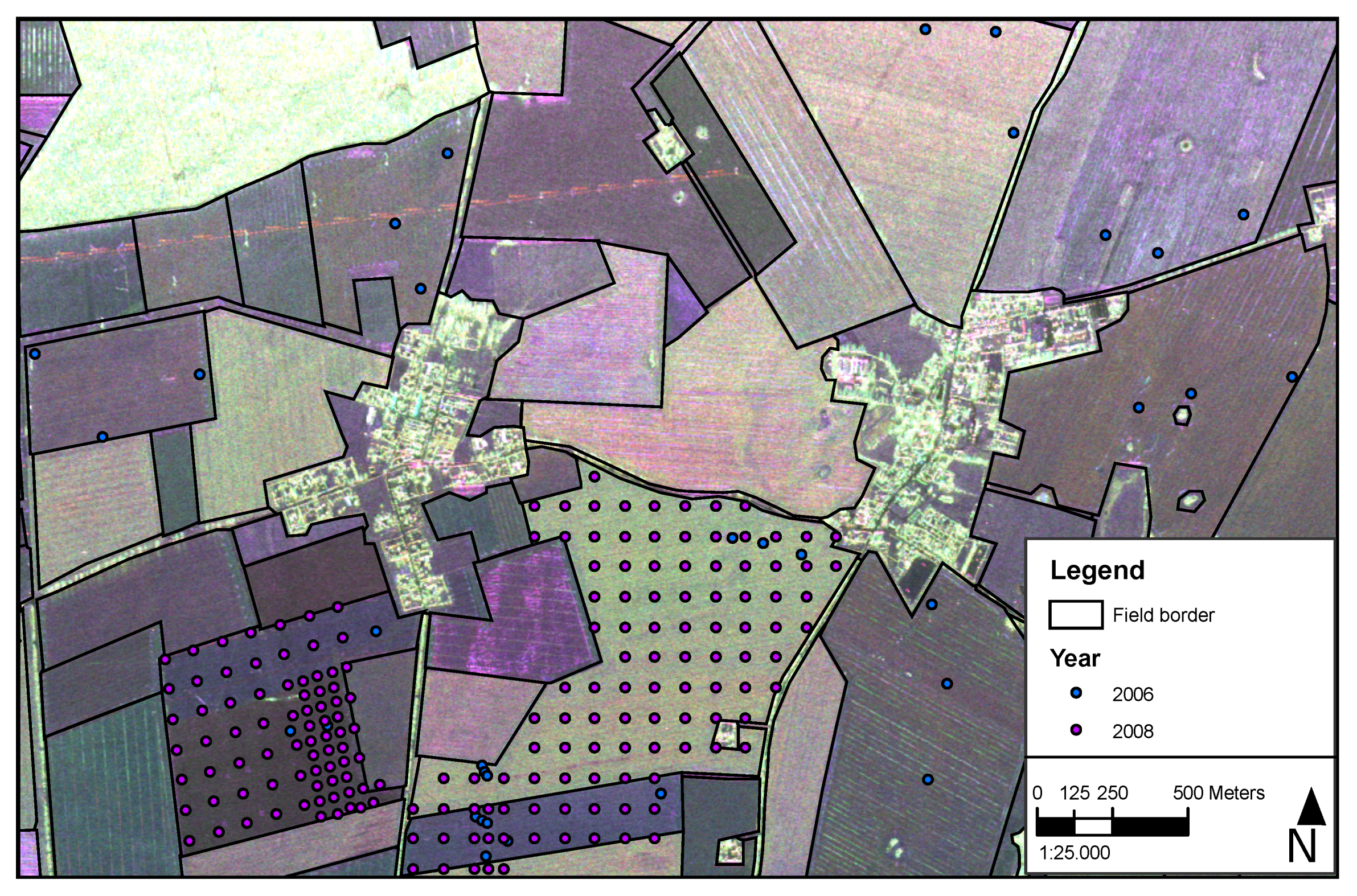
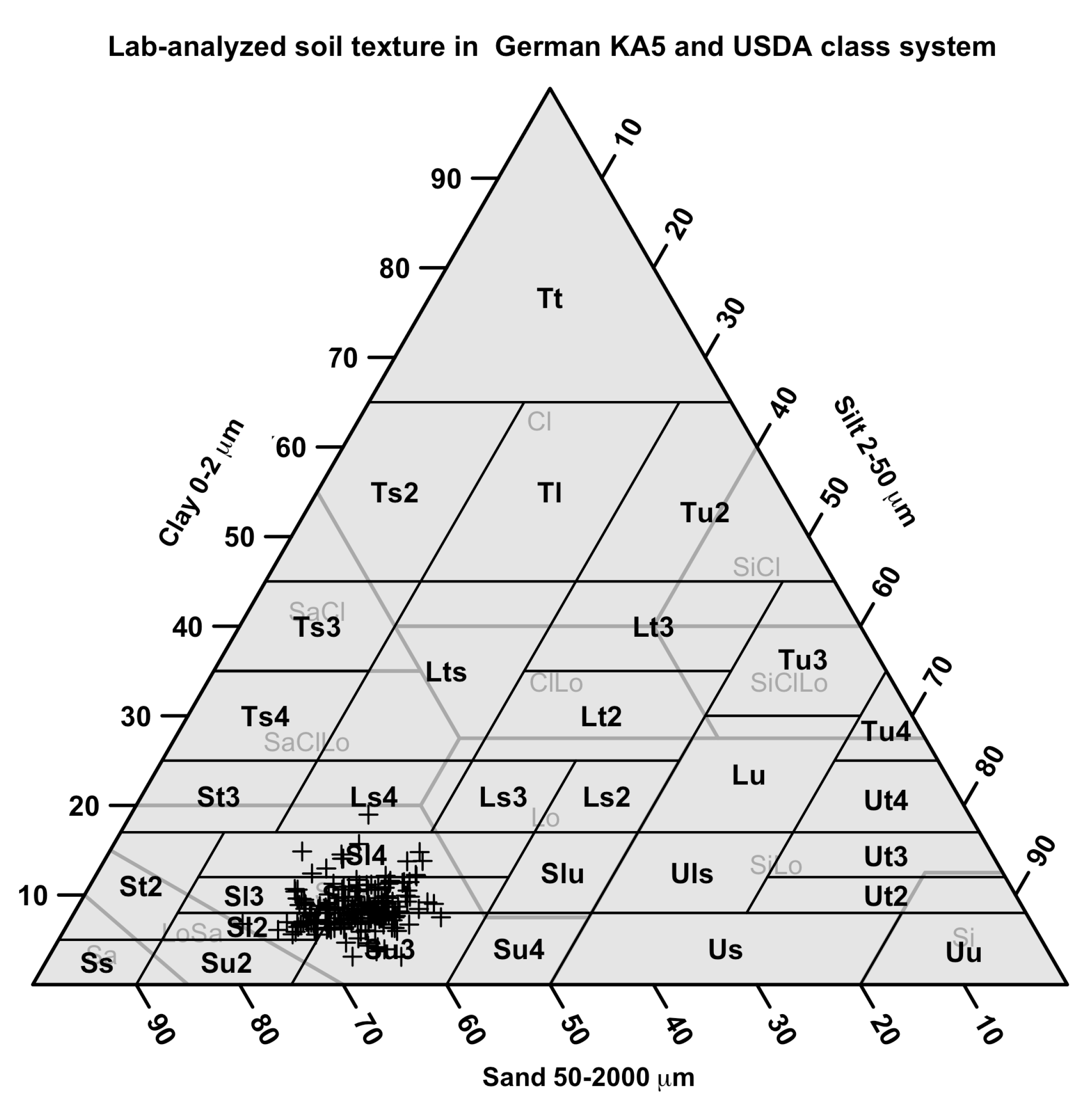
2.2. In-Field Data
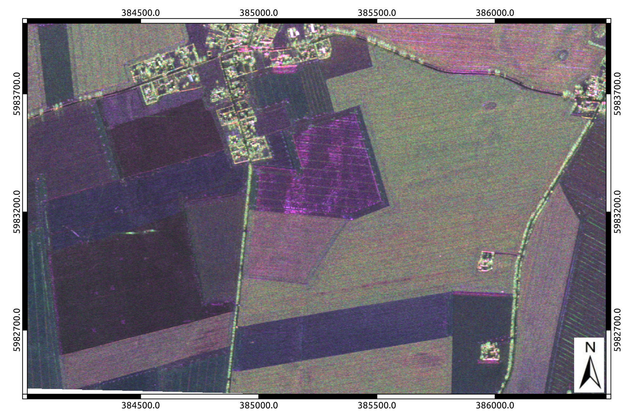
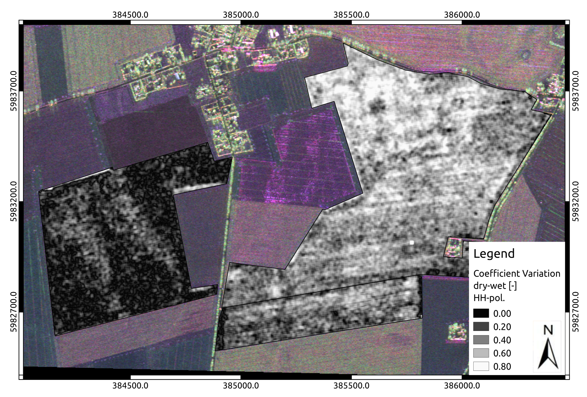
2.3. Remote Sensing Data
2.3.1. Processing of Remote Sensing Data Sets
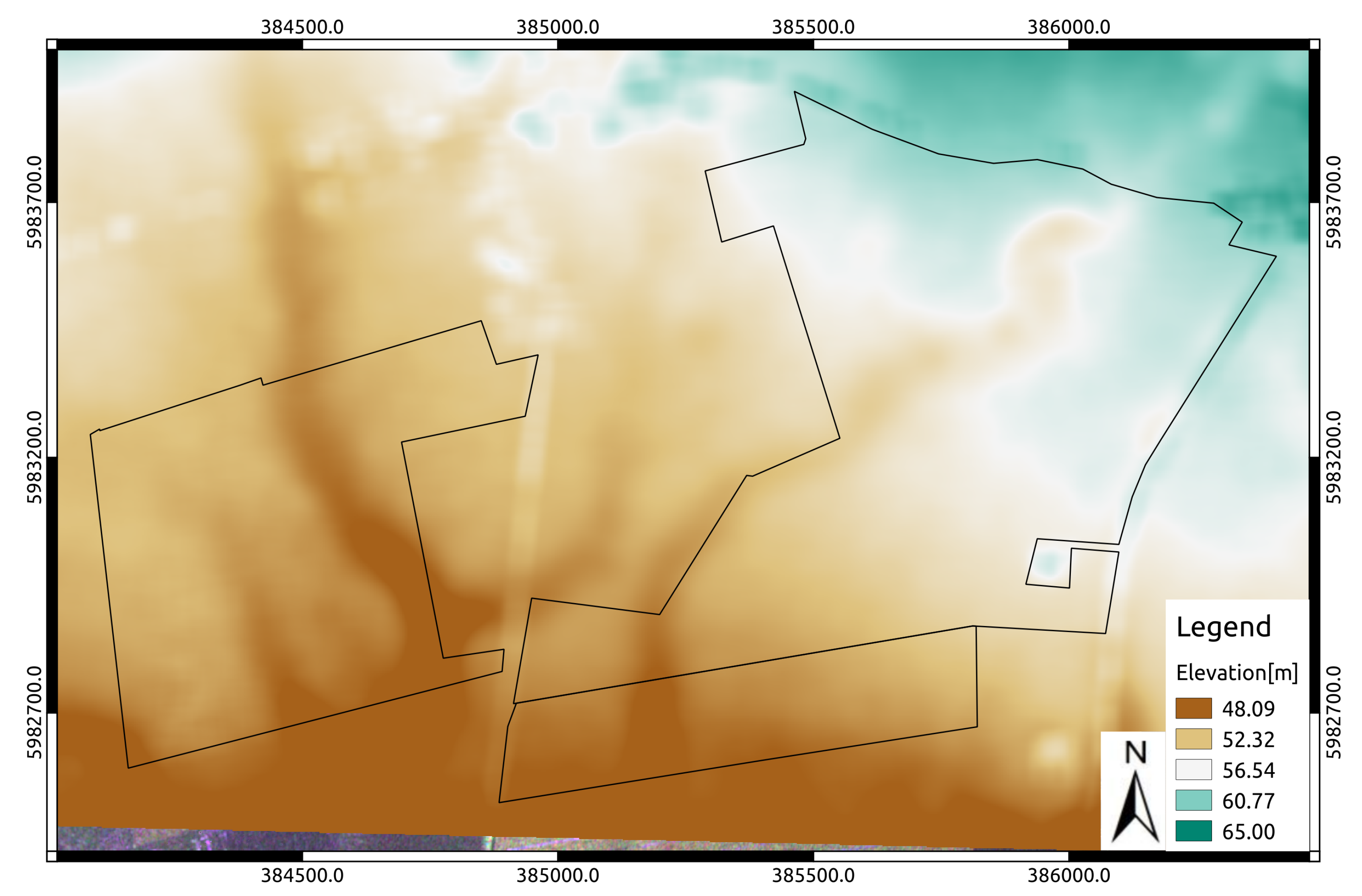
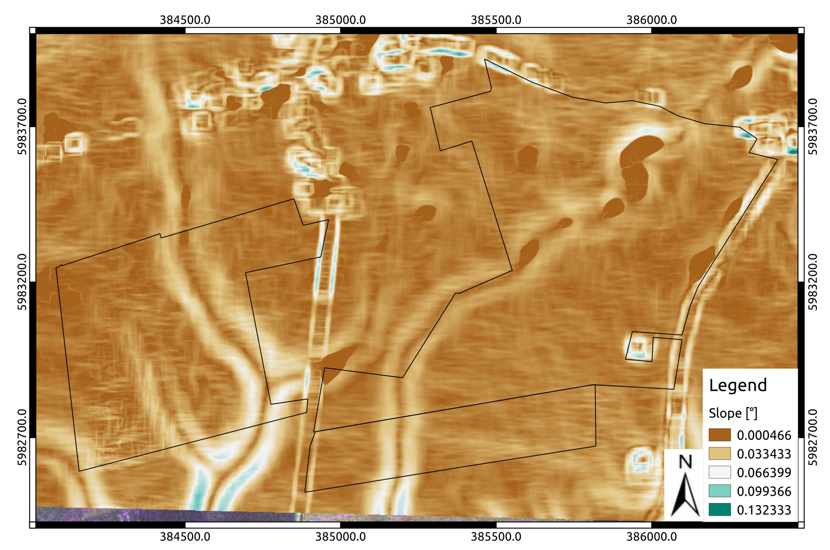
2.4. Additional Co-Variables
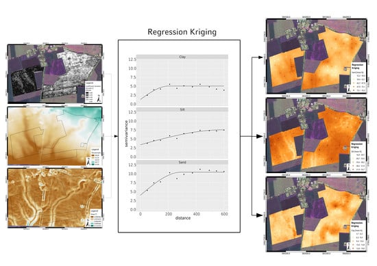
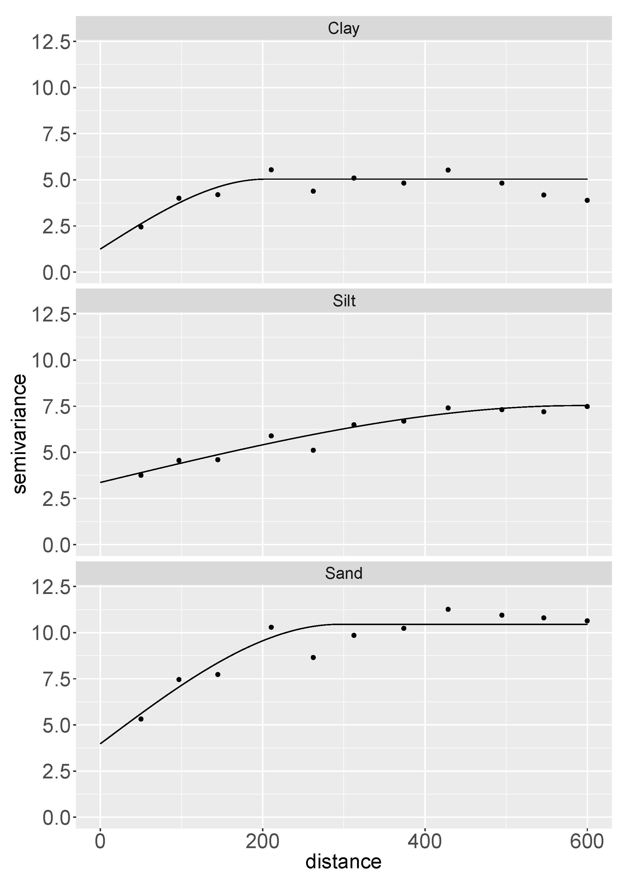
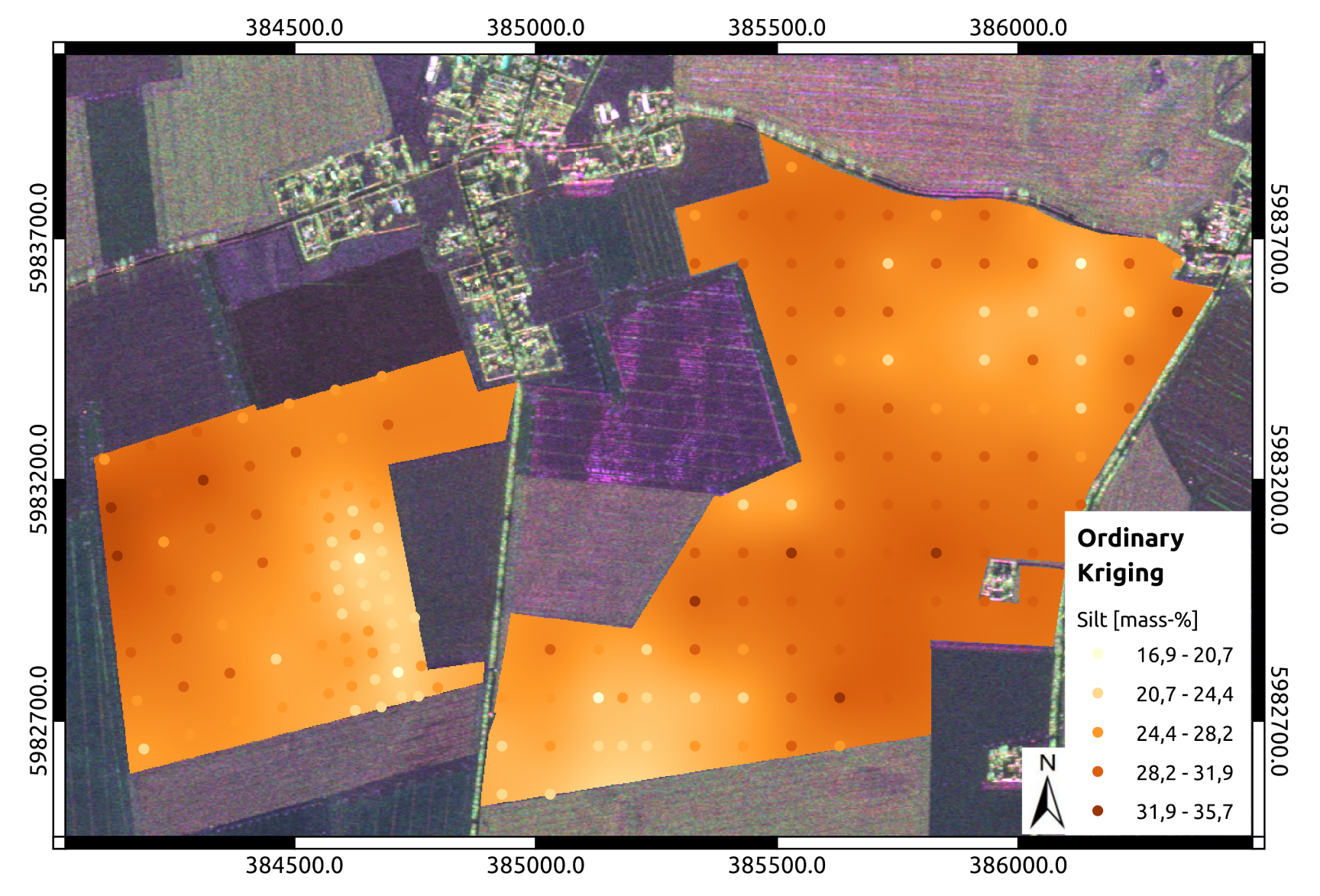
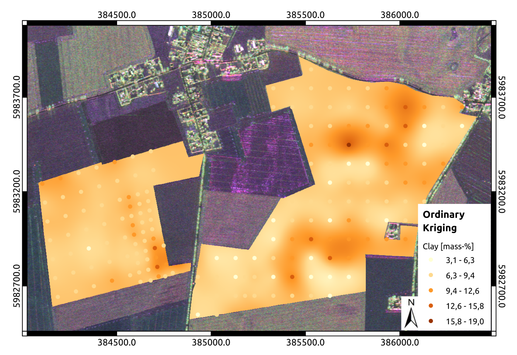
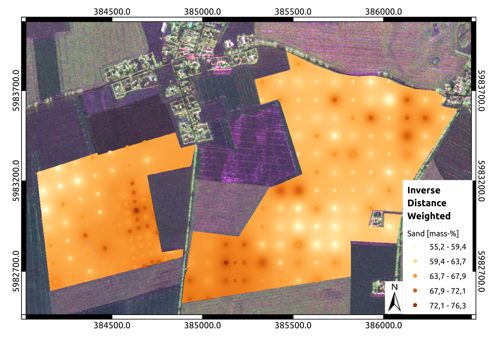
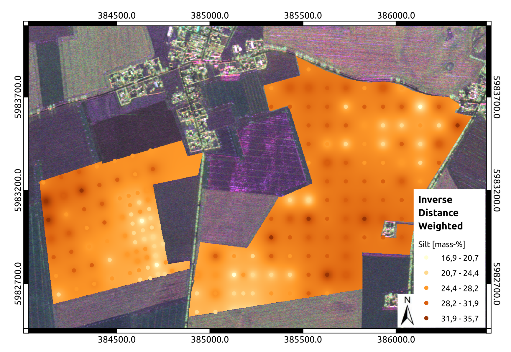
2.5. Geostatistical Approaches
2.6. Validation of the Model Performance
3. Results
4. Discussion
5. Conclusions
Author Contributions
Funding
Acknowledgments
Conflicts of Interest
References
- Vescovi, L.; Ludwig, R.; Cyr, J.F.; Turcotte, R.; Braun, M.; Fortin, L.-G.; Chaumont, D.; Braun, M.; Mauser, W. A Multi Model Experiment to Assessand Cope with Climate Change Impacts on the Chateauguay Watershed in Southern Quebec. Available online: https://unesdoc.unesco.org/ark:/48223/pf0000181888 (accessed on 18 August 2020).
- Ludwig, R.; May, I.; Turcotte, R.; Vescovi, L.; Braun, M.; Cyr, J.F.; Fortin, L.G.; Chaumont, D.; Biner, S.; Chartier, I.; et al. The role of hydrological model complexity and uncertainty in climate change impact assessment. Adv. Geosci. 2009, 21, 63–71. [Google Scholar] [CrossRef] [Green Version]
- Meyer, S. Climate Change Impact Assessment under Data Scarcity. Ph.D. Thesis, Ludwig-Maximilians-Universitaet (LMU), Munich, Germany, 2016. [Google Scholar]
- Park, S.; Vlek, P. Environmental correlation of three-dimensional soil spatial variability: A comparison of three adaptive techniques. Geoderma 2002, 103, 117–140. [Google Scholar] [CrossRef]
- Zhu, A.; MacKay, D. Effects of spatial detail of soil information on watershed modeling. J. Hydrol. 2001, 248, 54–77. [Google Scholar] [CrossRef] [Green Version]
- Meyer, S.; Blaschek, M.; Duttmann, R.; Ludwig, R. Improved hydrological model parametrization for climate change impact assessment under data scarcity: The potential of field monitoring teqhniques and geostatistics. Sci. Total. Environ. 2016, 543, 906–923. [Google Scholar] [CrossRef] [PubMed]
- Behrens, T.; Scholten, T. Digital soil mapping in Germany—A review. J. Plant Nutr. Soil Sci. 2006, 169, 434–443. [Google Scholar] [CrossRef]
- Loew, A.; Bell, W.; Brocca, L.; Bulgin, C.E.; Burdanowitz, J.; Calbet, X.; Donner, R.V.; Ghent, D.; Gruber, A.; Kaminski, T.; et al. Validation practices for satellite-based Earth observation data across communities. Rev. Geophys. 2017, 55, 779–817. [Google Scholar] [CrossRef] [Green Version]
- Kalman, R.E. A New Approach to Linear Filtering and Prediction Problems. Trans. ASME J. Basic Eng. 1960, 82, 35–45. [Google Scholar] [CrossRef] [Green Version]
- Schulz, K.; Beven, K.; Huwe, B. Equifinality and the Problem of Robust Calibration in Nitrogen Budget Simulations. Soil Sci. Soc. Am. J. 1999, 63, 1934–1941. [Google Scholar] [CrossRef]
- Dahlstrom, D.J. Calibration and Uncertainty Analysis for Complex Environmental Models. Ground Water 2015, 53, 673–674. [Google Scholar] [CrossRef]
- Webster, R. The development of pedometrics. Geoderma 1994, 62, 1–15. [Google Scholar] [CrossRef]
- Mcbratney, A.; Odeh, I.; Bishop, T.; Dunbar, M.; Shatar, T. An Overview of Pedometric Techniques for Use in Soil Survey. Geoderma 2000, 97, 293–327. [Google Scholar] [CrossRef]
- Hengl, T. A Practical Guide to Geostatistical Mapping. Available online: https://library.wur.nl/isric/fulltext/isricu_i27272_001.pdf (accessed on 18 August 2020).
- Hengl, T.; Heuvelink, G.B.; Rossiter, D.G. About regression-kriging: From equations to case studies. Comput. Geosci. 2007, 33, 1301–1315. [Google Scholar] [CrossRef]
- Krige, D.A. A Statistical Approach to Some Mine Valuation and Allied Problems on the Witwatersrad. Master’s Thesis, University of Witwatersrand, Johannesburg, South Africa, 1951. Unpublished. [Google Scholar]
- Matheron, G.; Blondel, F. Traité de Géostatistique Appliquée Tome I; Technip: Paris, France, 1962. [Google Scholar]
- Bishop, T.F.A.; McBratney, A.B. A comparison of prediction methods for the creation of field-extend soil property maps. Geoderma 2001, 103, 149–160. [Google Scholar] [CrossRef]
- Jenny, H. Factors of Soil Formation: A System of Quantitative Pedology; Dover Publications: New York, NY, USA, 1941. [Google Scholar]
- Dokuchaev, V.V. Russian Chernozems (Russkii Chernozems). Israel Prog. Sci. Trans., Jerusalem, Transl. from Russian by N. Kaner (1967); U.S. Dept. of Commerce: Springfield, VA, USA, 1883.
- Odeh, I.A.O.; McBratney, A.B.; Chittleborough, D.J. Further results on prediction of soil properties from terrain attributes: Heterotropic cokriging and regressionkrigign. Geoderma 1995, 67, 215266. [Google Scholar] [CrossRef]
- Dobos, E.; Micheli, E.; Baumgardner, M.; Biehl, L.; Helt, T. Use of combined digital elevation model and satellite radiometric data for regional soil mapping. Geoderma 2000, 97, 367–391. [Google Scholar] [CrossRef]
- Goovaerts, P. Geostatistical Approaches for Incorporating Elevation Into the Spatial Interpolation of Rainfall. J. Hydrol. 2000, 228, 113–129. [Google Scholar] [CrossRef]
- Krueger, K. Regionalisierung von Bodeneigenschaften unter Verwendung Digitaler Geländemodelle Sowie Multispektraler Fernerkundungsdaten am Beispile einer Agrarlandschaft im Jungmoränengebiet Schleswig-Holsteins. Ph.D. Thesis, Christian-Albrechts-Universität Kiel, Kiel, Germany, 2008. [Google Scholar]
- Zhu, A.X.; Liu, F.; Li, B.; Pei, T.; Qin, C.; Liu, G.; Wang, Y.; Chen, Y.; Ma, X.; Qi, F.; et al. Differentiation of Soil Conditions over Low Relief Areas Using Feedback Dynamic Patterns. Soil Sci. Soc. Am. J. 2010, 74, 861–869. [Google Scholar] [CrossRef] [Green Version]
- Zhang, Y.; Guo, L.; Chen, Y.; Shi, T.; Luo, M.; Ju, Q.; Zhang, H.; Wang, S. Prediction of Soil Organic Carbon based on Landsat 8 Monthly NDVI Data for the Jianghan Plain in Hubei Province, China. Remote Sens. 2019, 11, 1683. [Google Scholar] [CrossRef] [Green Version]
- Reuter, H.I. Spatial Crop and Soil Landscape Processes under Special Consideration of Relief Information in a Loess Landscape. Ph.D. Thesis, University of Hannover, Hannover, Germany, 2004. [Google Scholar]
- MCBratney, A.B.; Pringle, M.J. Chapter Spatial Variability in Soil-Implications for Precision Agriculture. Proc. Precis. Agric. 1997, 1997, 3–31. [Google Scholar]
- Werner, A.; Jarfe, A.; Auernhammer, A.; Basso, B.; Bill, R. Precision Agriculture: Herausforderung an Integrative Forschung, Emtwicklung und Anwendung in der Praxis; Zentrum für Agrarlandschafts und Landnutzungsforschung: Müncheberg, Germany, 2002. [Google Scholar]
- Huete, A.R.; Liu, H.Q. An error and sensitivity analysis of the atmospheric- and soil-correcting variants of the NDVI for the MODIS-EOS. IEEE Trans. Geosci. Remote Sens. 1994, 32, 897–905. [Google Scholar] [CrossRef]
- Rondeaux, G.; Steven, M.; Baret, F. Optimization of soil-adjusted vegetation indices. Remote Sens. Environ. 1996, 55, 95–107. [Google Scholar] [CrossRef]
- Pettorelli, N.; Vik, J.O.; Mysterud, A.; Gaillard, J.M.; Tucker, C.J.; Stenseth, N.C. Using the satellite-derived NDVI to assess ecological responses to environmental change. Trends Ecol. Evol. 2005, 20, 503–510. [Google Scholar] [CrossRef] [PubMed]
- McKenzie, N.J.; Ryan, P.J. Spatial prediction of soil properties using environmental correlation. Geoderma 1999, 89, 67–94. [Google Scholar] [CrossRef]
- Sumfleth, K.; Duttmann, R. Prediction of soil property distribution in paddy soil landscapes using terrain data and satellite information as indicators. Ecol. Indic. 2008, 8, 485–501. [Google Scholar] [CrossRef]
- Moreira, A.; Prats-Iraola, P.; Younis, M.; Krieger, G.; Hajnsek, I.; Papathanassiou, K.P. A tutorial on synthetic aperture radar. IEEE Geosci. Remote. Sens. Mag. 2013, 1, 6–43. [Google Scholar] [CrossRef] [Green Version]
- Ulaby, F.T.; Long, D.G.; Blackwell, W.J.; Elachi, C.; Fung, A.K.; Ruf, C.; Sarabandi, K.; Zebker, H.A.; Van Zyl, J. Microwave Radar and Radiometric Remote Sensing; University of Michigan Press: Ann Arbor, MI, USA, 2014; Volume 4. [Google Scholar]
- Dobson, M.C.; Ulaby, F. Microwave Backscatter Dependence on Surface Roughness, Soil Moisture, And Soil Texture: Part III-Soil Tension. IEEE Trans. Geosci. Remote Sens. 1981, GE-19, 51–61. [Google Scholar] [CrossRef]
- Santanello, J.A., Jr.; Peters-Lidard, C.D.; Garcia, M.E.; Mocko, D.M.; Tischler, M.A.; Moran, M.S.; Thoma, D. Using remotely-sensed estimates of soil moisture to infer soil texture and hydraulic properties across a semi-arid watershed. Remote Sens. Environ. 2007, 110, 79–97. [Google Scholar] [CrossRef] [Green Version]
- Baghdadi, N.; Zribi, M.; Loumagne, C.; Ansart, P.; Anguela, T.P. Analysis of TerraSAR-X data and their sensitivity to soil surface parameters over bare agricultural fields. Remote Sens. Environ. 2008, 112, 4370–4379. [Google Scholar] [CrossRef] [Green Version]
- Zribi, M.; Kotti, F.; Lili-Chabaane, Z.; Baghdadi, N.; Ben Issa, N.; Amri, R.; Amri, B.; Chehbouni, A. Soil Texture Estimation Over a Semiarid Area Using TerraSAR-X Radar Data. IEEE Geosci. Remote. Sens. Lett. 2012, 9, 353–357. [Google Scholar] [CrossRef] [Green Version]
- Gorrab, A.; Zribi, M.; Baghdadi, N.; Mougenot, B.; Fanise, P.; Chabaane, Z. Retrieval of Both Soil Moisture and Texture Using TerraSAR-X Images. Remote Sens. 2015, 7, 10098–10116. [Google Scholar] [CrossRef] [Green Version]
- Bousbih, S.; Zribi, M.; Pelletier, C.; Gorrab, A.; Lili-Chabaane, Z.; Baghdadi, N.; Ben Aissa, N.; Mougenot, B. Soil Texture Estimation Using Radar and Optical Data from Sentinel-1 and Sentinel-2. Remote Sens. 2019, 11, 1520. [Google Scholar] [CrossRef] [Green Version]
- Marzahn, P.; Ludwig, R. On the derivation of soil surface roughness from multi-parametric PolSAR data and its potential for hydrological modeling. Hydrol. Earth Syst. Sci. 2009, 13, 381–394. [Google Scholar] [CrossRef] [Green Version]
- Hurtig, T. Physische Geographie von Mecklenburg; VEB Deutscher Verlag: Berlin, Germany, 1957. [Google Scholar]
- LUNG. Beiträge zum Bodenschutz in Mecklenburg- Vorpommern, Böden in Mecklenburg- Vorpommern- Abriss ihrer Entstehung, Verbreitung und Nutzung; Landesamt für Umwelt, Naturschutz und Geologie Mecklenburg: Vorpommern, Germany, 2005. [Google Scholar]
- Helbig, H. Die spätglaziale und holozäne Überprägung der Grundmoränenplatten in Vorpommern. Ph.D. Thesis, University of Greifswald, Greifswald, Germany, 1999. [Google Scholar]
- Billwitz, K.; Michaelis, D.; Succow, M. Landschaftsökologische Exkursionen in die Greifswalder Umgebung; University of Greifswald: Greifswald, Germany, 2003. [Google Scholar]
- Scheiber, R.; Keller, M.; Fischer, J.; Andres, C.; Horn, R.; Hajnsek, I. Radar data processing, quality analysis and level-1b product generation for AGRISAR and EAGLE campaigns. In Proceedings of the AGRISAR and EAGLE Campaigns Final Workshop—ESA/ESTEC-2007, Noordwijk, The Netherlands, 15–16 October 2007. [Google Scholar]
- Lee, J.S.; Grunes, M.; de Grandi, G. Polarimetric SAR speckle filtering and its implication for classification. IEEE Trans. Geosci. Remote Sens. 1999, 37, 2363–2373. [Google Scholar] [CrossRef]
- Conrad, O.; Bechtel, B.; Bock, M.; Dietrich, H.; Fischer, E.; Gerlitz, L.; Wehberg, J.; Wichmann, V.; Böhner, J. System for Automated Geoscientific Analyses (SAGA) v. 2.1.4. Geosci. Model Dev. 2015, 8, 1991–2007. [Google Scholar] [CrossRef] [Green Version]
- Beven, K.J.; Kirkby, M.J. A physically based variable contribution area model of basin hydrology. Hydrol. Sci. Bull. 1979, 24, 43–69. [Google Scholar] [CrossRef] [Green Version]
- Boehner, J.; Selige, T. SAGA—Analysis and Modelling Applications. In Goettinger Geographische Abhandlungen; University of Göttingen: Göttingen, Germany, 2006. [Google Scholar]
- Moore, I.D.; Gessler, P.E.; Nielsen, G.A.; Peterson, G.A. Soil Attribute Prediction Using Terrain Analyses. Soil Sci. Soc. Am. J. 1993, 57, 443–452. [Google Scholar] [CrossRef]
- Olaya, V. A Gentle Introduction to SAGA GIS. Available online: https://deac-ams.dl.sourceforge.net/project/saga-gis/SAGA%20-%20Documentation/SAGA%20Documents/SagaManual.pdf (accessed on 18 August 2020).
- Conrad, O. SAGA Entwurf, Funktionsumfang und Anwendung eines Systems für Automatisierte Geowissenschaftliche Analysen. Ph.D. Thesis, University of Göttingen, Göttingen, Germany, 2006. [Google Scholar]
- Adhikari, K.; Kheir, R.B.; Greve, M.B.; Greve, M.H. Comparing kriging and regression approaches for mapping soil clay content in a diverse Danish landscape. Soil Sci. 2013, 178, 505–517. [Google Scholar] [CrossRef]
- Goovaerts, P. Geostatistics for Natural Resources Evaluation; Oxford University Press: Oxford, UK, 1997. [Google Scholar]
- Webster, R.; Oliver, M.A. Geostatistics for Environmental Scientists, 2nd ed.; John Wiley and Sons, Ltd.: Chichester, UK, 2007; p. 315. [Google Scholar]
- Keskin, H.; Grunwald, S. Regression kriging as a workhorse in the digital soil mapper’s toolbox. Geoderma 2018, 326, 22–41. [Google Scholar] [CrossRef]
- Matheron, G. The Theory of Regionalized Variables and its Applications; École National Supérieure des Mines: Paris, France, 1971; Volume 5, p. 211. [Google Scholar]
- Venables, W.N.; Ripley, B.D. Modern Applied Statistics with S, 4th ed.; Springer: New York, NY, USA, 2002; ISBN 0-387-95457-0. [Google Scholar]
- R Core Team. R: A Language and Environment for Statistical Computing; R Foundation for Statistical Computing: Vienna, Austria, 2020. [Google Scholar]
- Isaaks, E.H.; Srivastava, R.M. An Introduction to Applied Geostatistics; Oxford University Press: Oxford, UK, 1989; Volume 17, pp. 471–473. [Google Scholar] [CrossRef]
- Chai, T.; Draxler, R. Root mean square error (RMSE) or mean absolute error (MAE)?– Arguments against avoiding RMSE in the literature. Geosci. Model Dev. 2014, 7, 1247–1250. [Google Scholar] [CrossRef] [Green Version]
- Mattia, F.; Le Toan, T.; Picard, G.; Posa, F.I.; D’Alessio, A.; Notarnicola, C.; Gatti, A.M.; Rinaldi, M.; Satalino, G.; Pasquariello, G. Multitemporal C-band radar measurements on wheat fields. IEEE Trans. Geosci. Remote Sens. 2003, 41, 1551–1560. [Google Scholar] [CrossRef]
- Lievens, H.; Verhoest, N.E. Spatial and temporal soil moisture estimation from RADARSAT-2 imagery over Flevoland, The Netherlands. J. Hydrol. 2012, 456–457, 44–56. [Google Scholar] [CrossRef]
- Hengl, T.; de Jesus, J.M.; MacMillan, R.A.; Batjes, N.H.; Heuvelink, G.B.M.; Ribeiro, E.; Samuel-Rosa, A.; Kempen, B.; Leenaars, J.G.B.; Walsh, M.G.; et al. SoilGrids1km—Global Soil Information Based on Automated Mapping. PLoS ONE 2014, 9, e105992. [Google Scholar] [CrossRef] [PubMed] [Green Version]
- Berger, M.; Moreno, J.; Johannessen, J.A.; Levelt, P.F.; Hanssen, R.F. ESA’s sentinel missions in support of Earth system science. Remote Sens. Environ. 2012, 120, 84–90. [Google Scholar] [CrossRef]
- Malenovský, Z.; Rott, H.; Cihlar, J.; Schaepman, M.E.; García-Santos, G.; Fernandes, R.; Berger, M. Sentinels for science: Potential of Sentinel-1, -2, and -3 missions for scientific observations of ocean, cryosphere, and land. Remote Sens. Environ. 2012, 120, 91–101. [Google Scholar] [CrossRef]
- Ulaby, F.T.; Long, D. Microwave Radar and Radiometric Remote Sensing; University of Michigan Press: Ann Arbor, MI, USA, 2014. [Google Scholar]


| Year | n | Soil Texture | Ctot | N | Bulk Density | Soil Moisture | Soil Surface Roughness |
|---|---|---|---|---|---|---|---|
| 2006 | 27 | x | x | x | x | ||
| 2008 | 400 | x | x | x |
| Texture Class | Mean [Mass-%] | Min [Mass-%] | Max [Mass-%] | std [Mass-%] | cv |
|---|---|---|---|---|---|
| sand | 63 | 44 | 76 | 5.1 | 8.1 |
| silt | 27 | 16 | 36 | 3.6 | 13.4 |
| clay | 9 | 3 | 26 | 4.1 | 41.5 |
| Texture Class | Best Fit MLR-Model | RMSE |
|---|---|---|
| Sand | −041 ∗ DEM + 4179 ∗ + 0.88 ∗ CNBL + 85.32 | 3.24 |
| Silt | 0.37 ∗ DEM + 8.92 ∗ LS − 2.70 ∗ − 190.75 ∗ − 1.14 ∗ CNBL − 0.48 ∗ TWI + 14.92 | 2.65 |
| Clay | 6.23 ∗ ACN − 11.12 ∗ LS + 155.47 ∗ + 2.43 ∗ + 0.4 ∗ TWI − 1.49 | 2.19 |
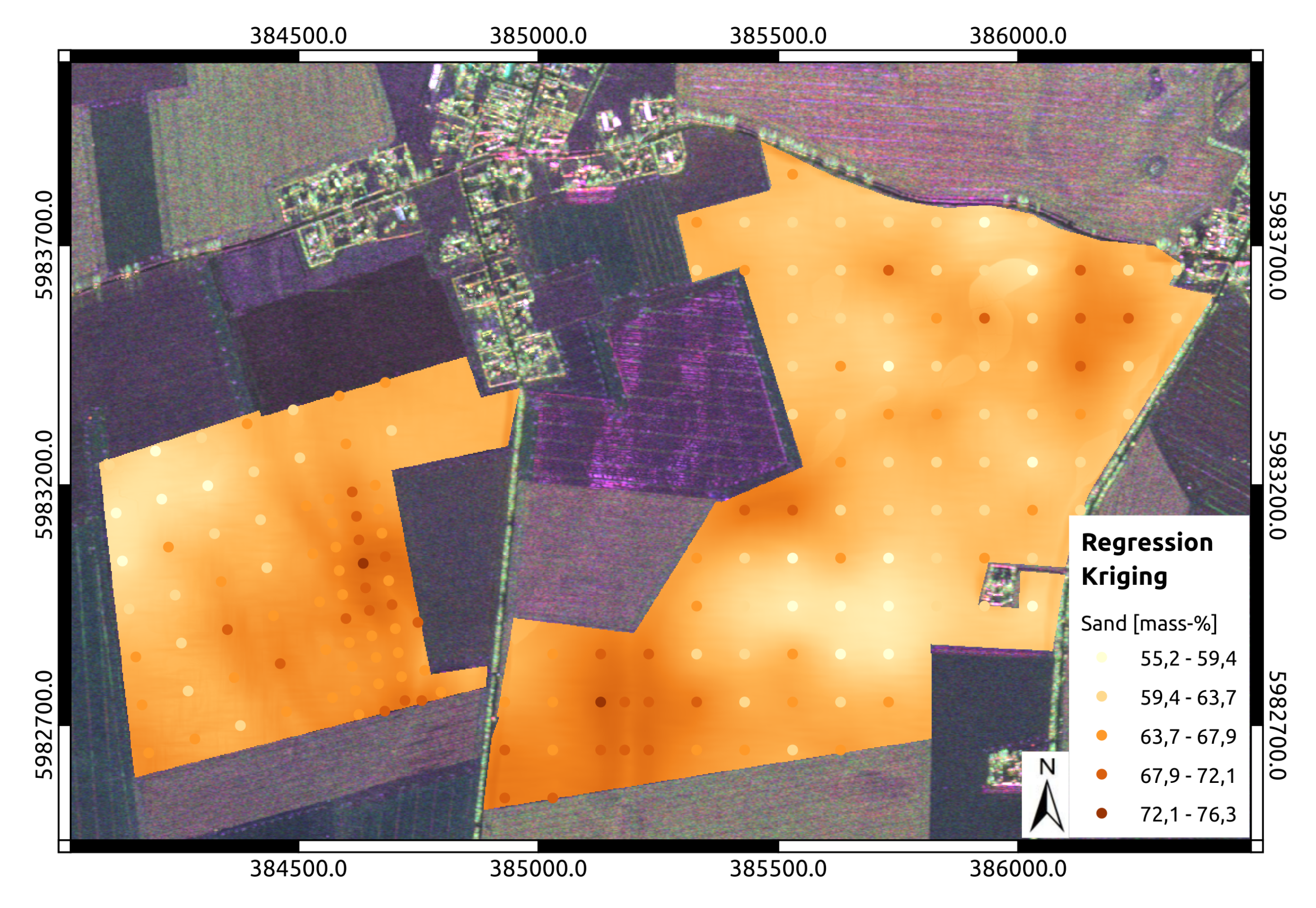
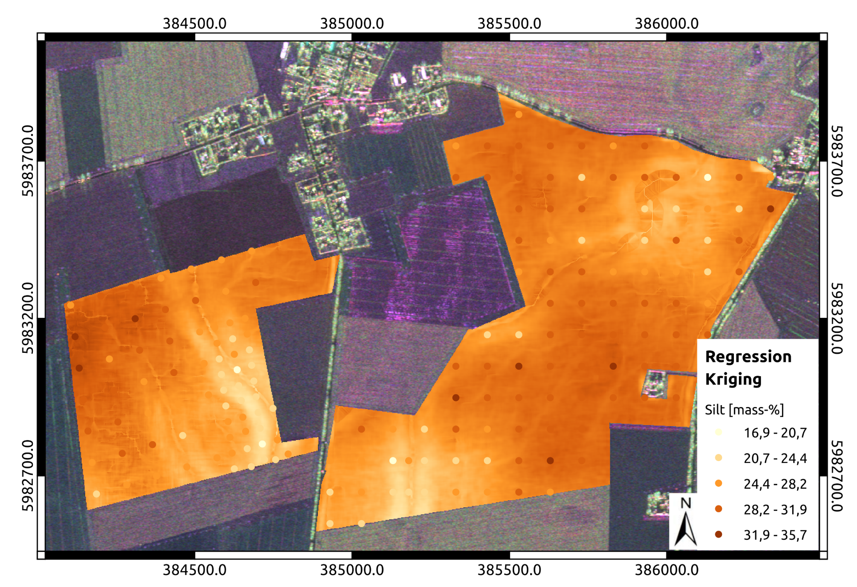
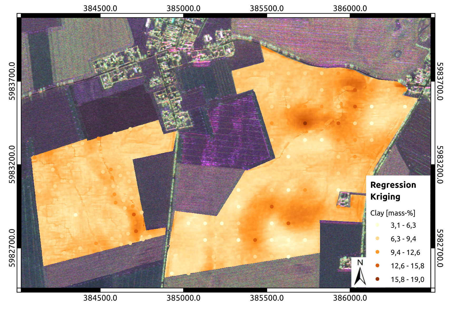
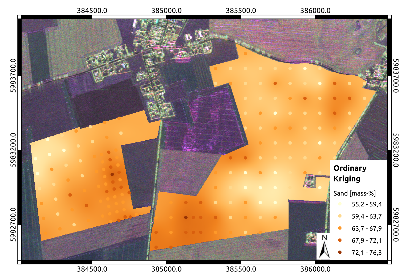
| Texture Class | RK | OK | IDW |
|---|---|---|---|
| Sand | 2.85 * | 2.86 * | 2.93 * |
| Silt | 2.31 * | 2.42 * | 2.54 * |
| Clay | 2.12 * | 2.22 * | 2.26 * |
| mean | 2.43 | 2.51 | 2.57 |
© 2020 by the authors. Licensee MDPI, Basel, Switzerland. This article is an open access article distributed under the terms and conditions of the Creative Commons Attribution (CC BY) license (http://creativecommons.org/licenses/by/4.0/).
Share and Cite
Marzahn, P.; Meyer, S. Utilization of Multi-Temporal Microwave Remote Sensing Data within a Geostatistical Regionalization Approach for the Derivation of Soil Texture. Remote Sens. 2020, 12, 2660. https://0-doi-org.brum.beds.ac.uk/10.3390/rs12162660
Marzahn P, Meyer S. Utilization of Multi-Temporal Microwave Remote Sensing Data within a Geostatistical Regionalization Approach for the Derivation of Soil Texture. Remote Sensing. 2020; 12(16):2660. https://0-doi-org.brum.beds.ac.uk/10.3390/rs12162660
Chicago/Turabian StyleMarzahn, Philip, and Swen Meyer. 2020. "Utilization of Multi-Temporal Microwave Remote Sensing Data within a Geostatistical Regionalization Approach for the Derivation of Soil Texture" Remote Sensing 12, no. 16: 2660. https://0-doi-org.brum.beds.ac.uk/10.3390/rs12162660