Shoreline Extraction from WorldView2 Satellite Data in the Presence of Foam Pixels Using Multispectral Classification Method


Abstract
:
1. Introduction
2. Materials and Methods
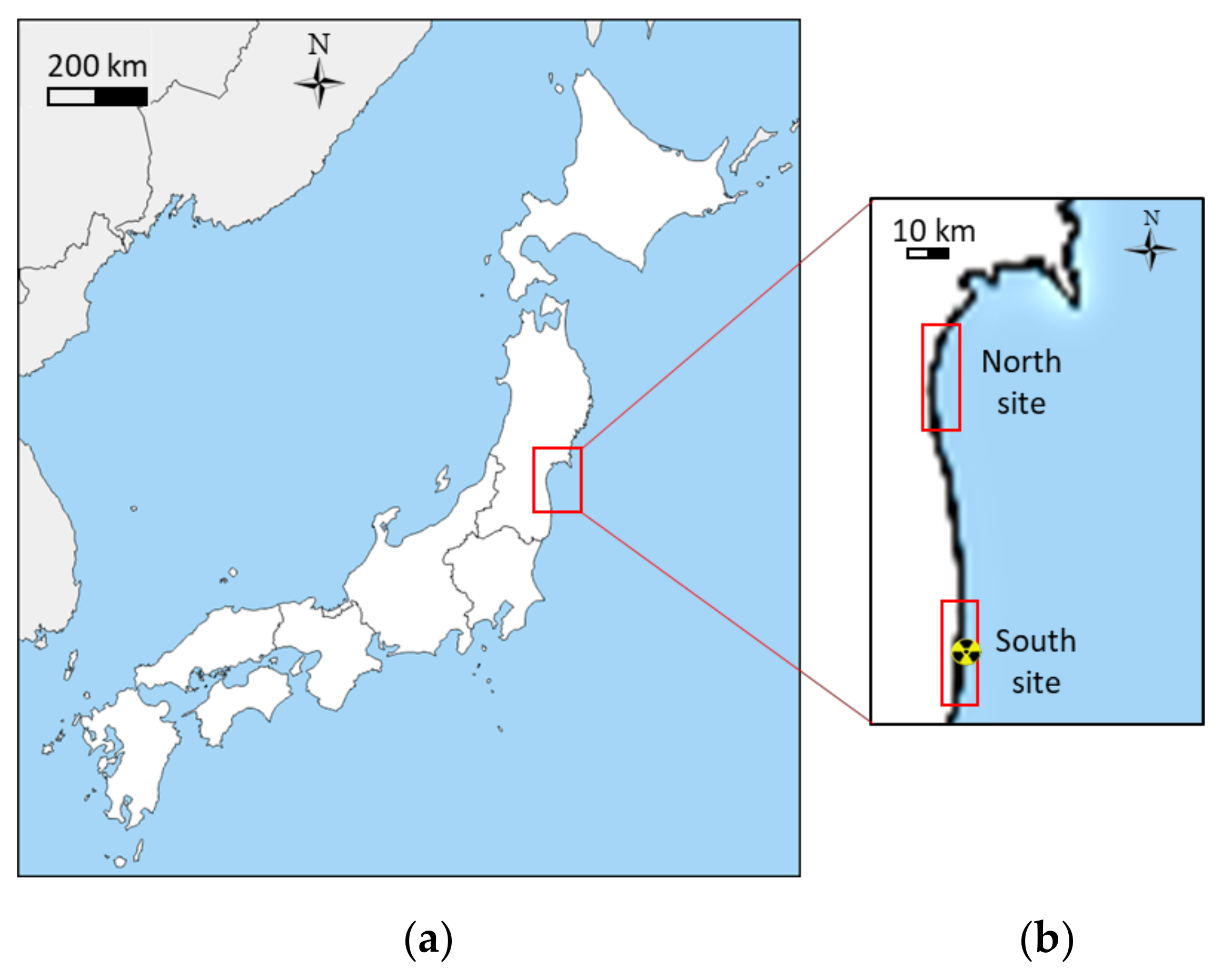
2.1. Study Area
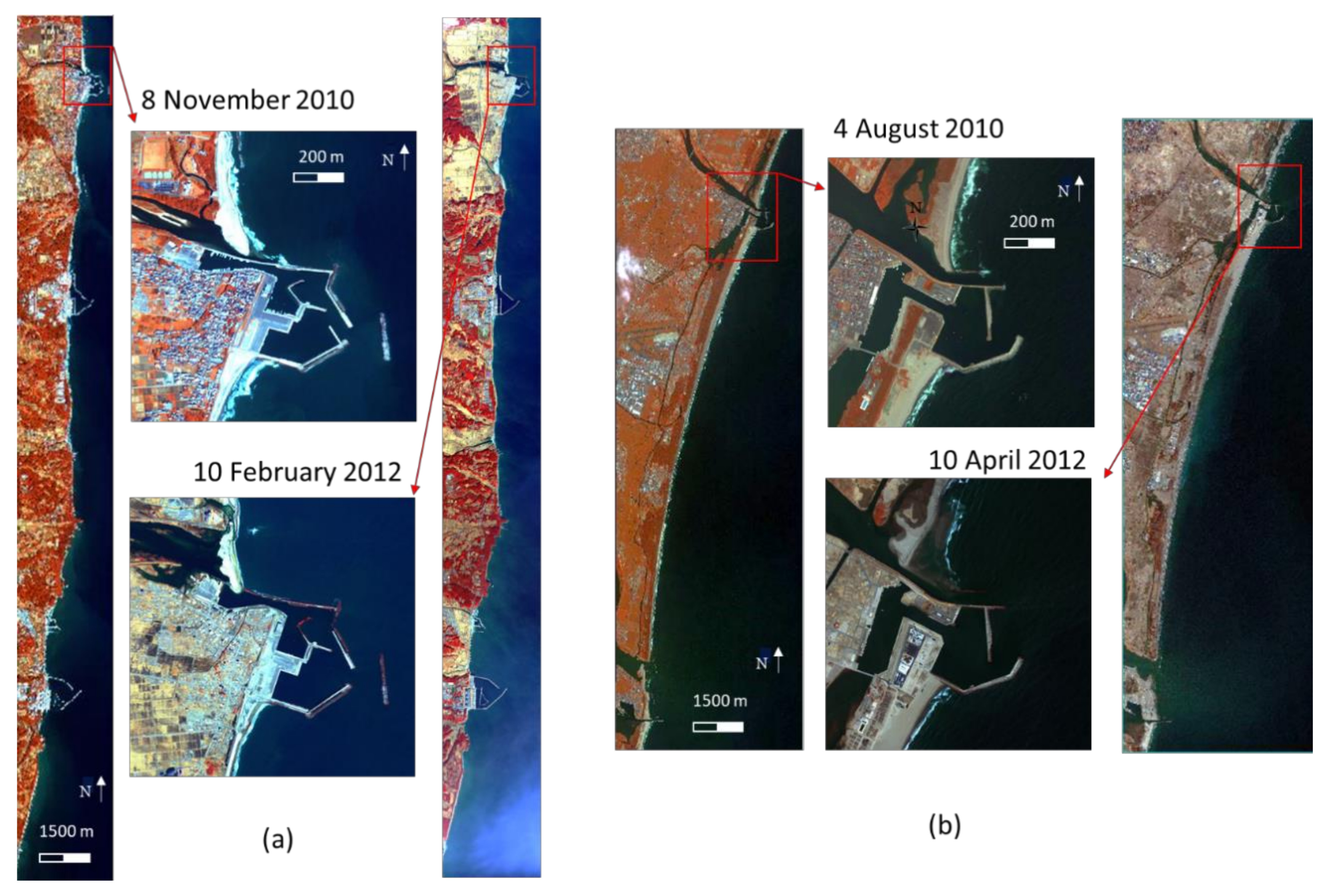
2.2. Satellite Data
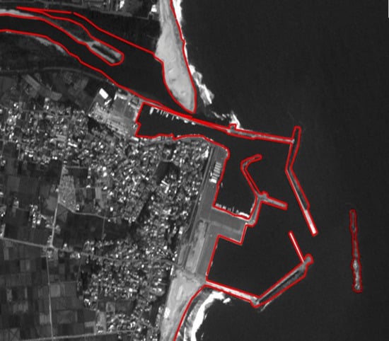
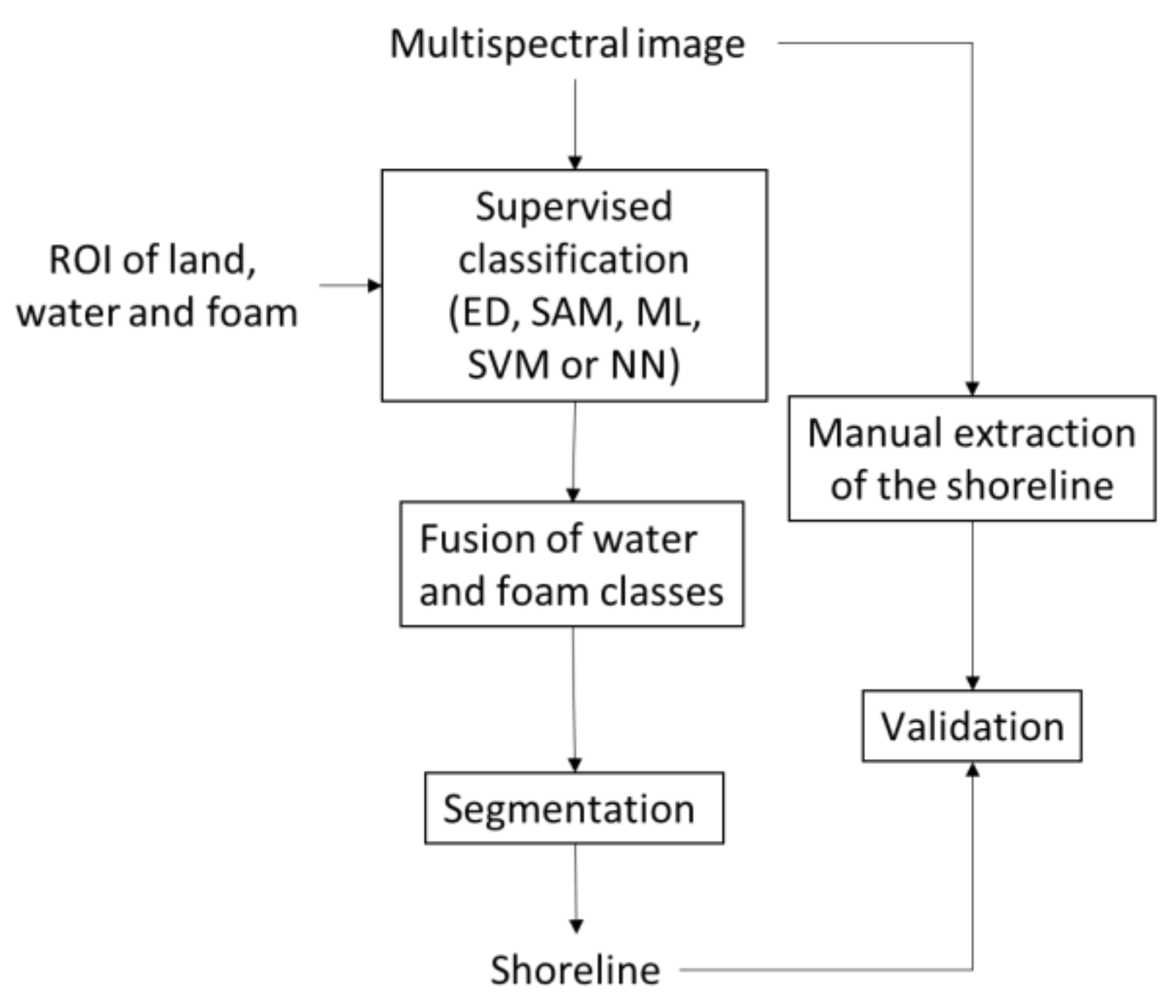
2.3. Methodology
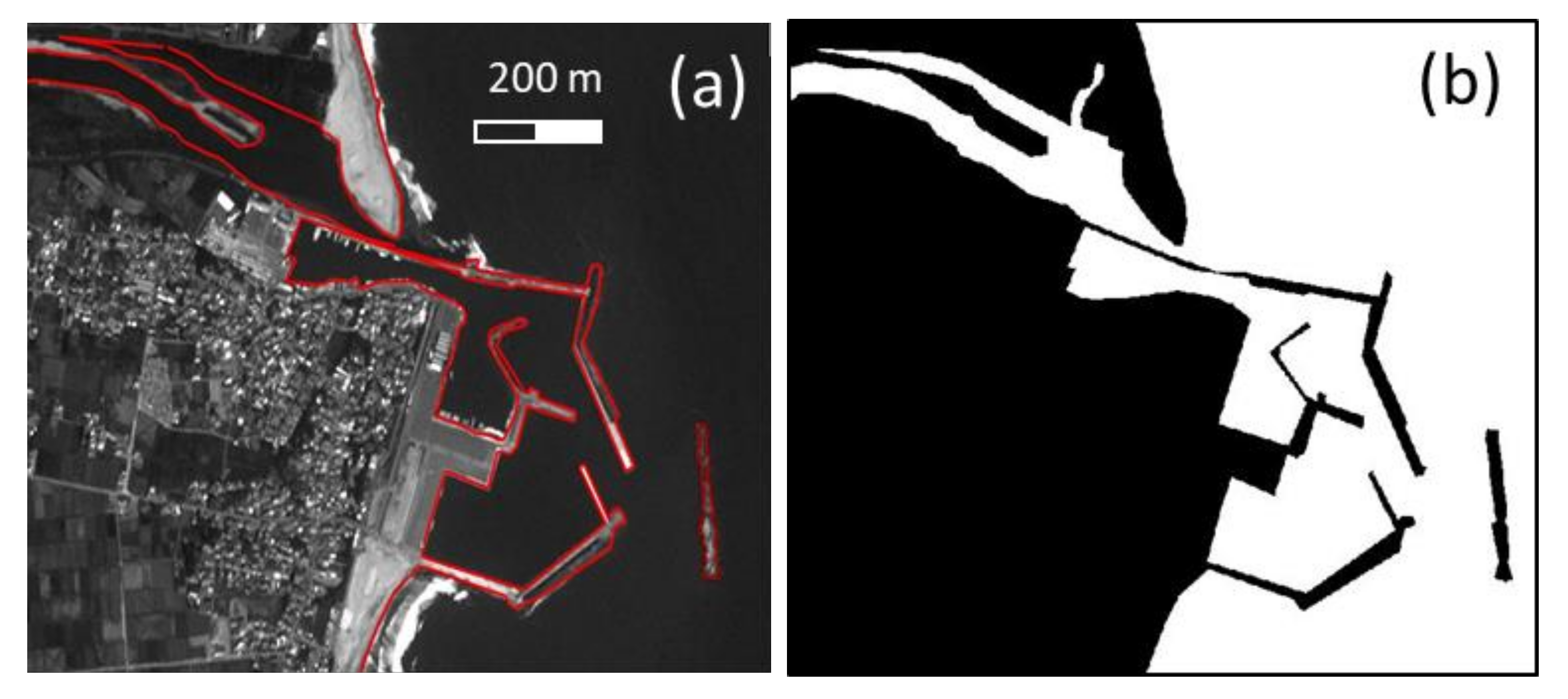
2.4. Validation
- -
- the comparison between land/ocean maps for each classification and the reference map; such a comparison provides estimates of false positive and false negative errors.
- -
- the comparison between the erosion and accretion surface areas estimated for each classification and the reference values.
2.4.1. False Positive and False Negative Errors
2.4.2. Erosion and Accretion
3. Results
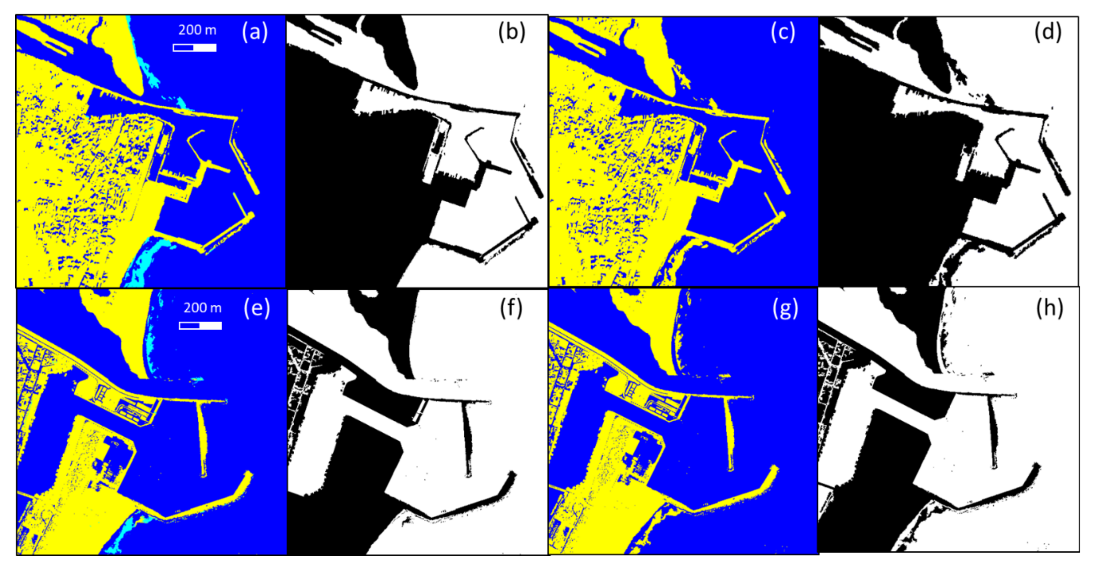
Importance of the Consideration of the Foam Class
4. Discussion
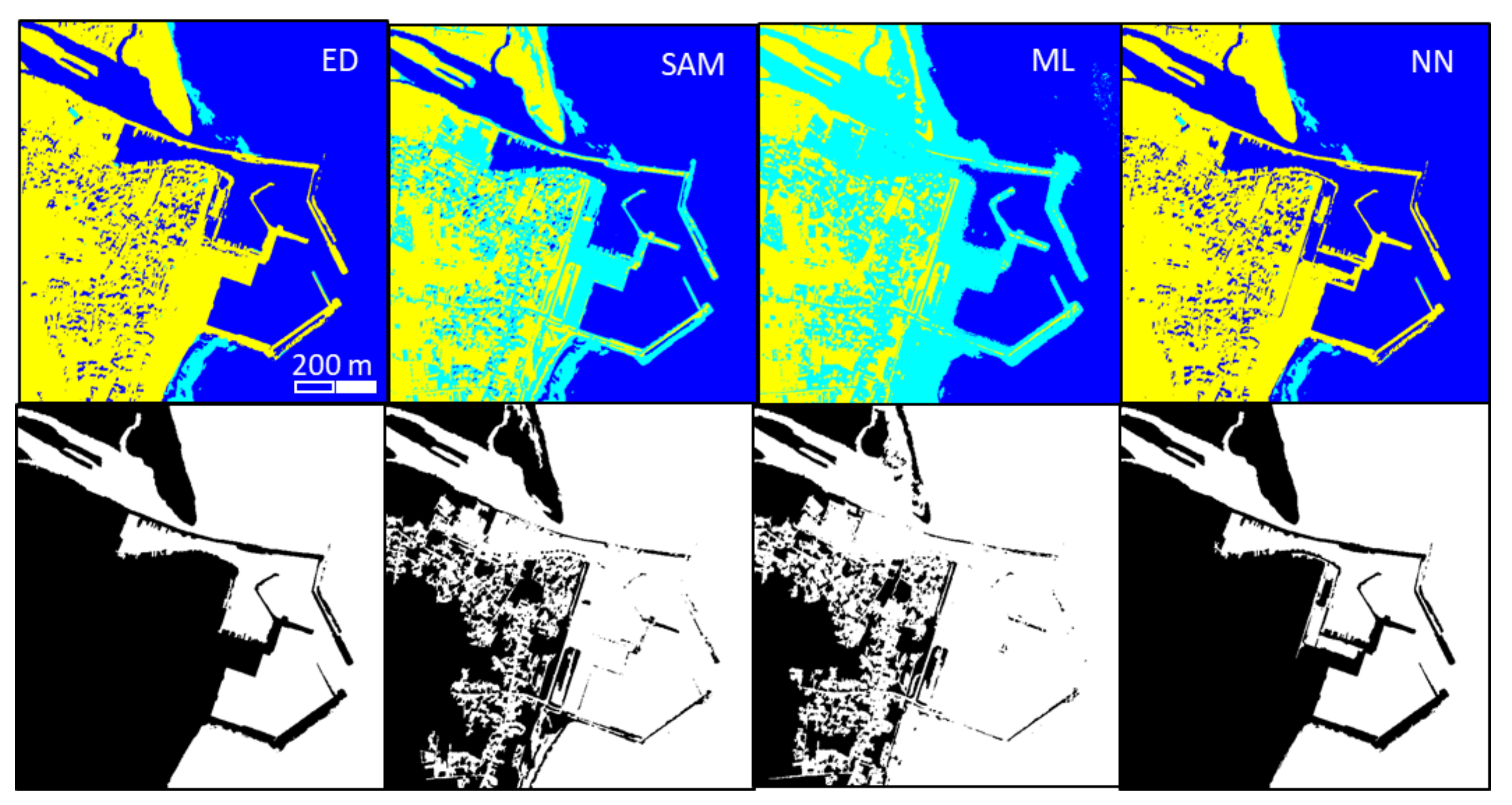
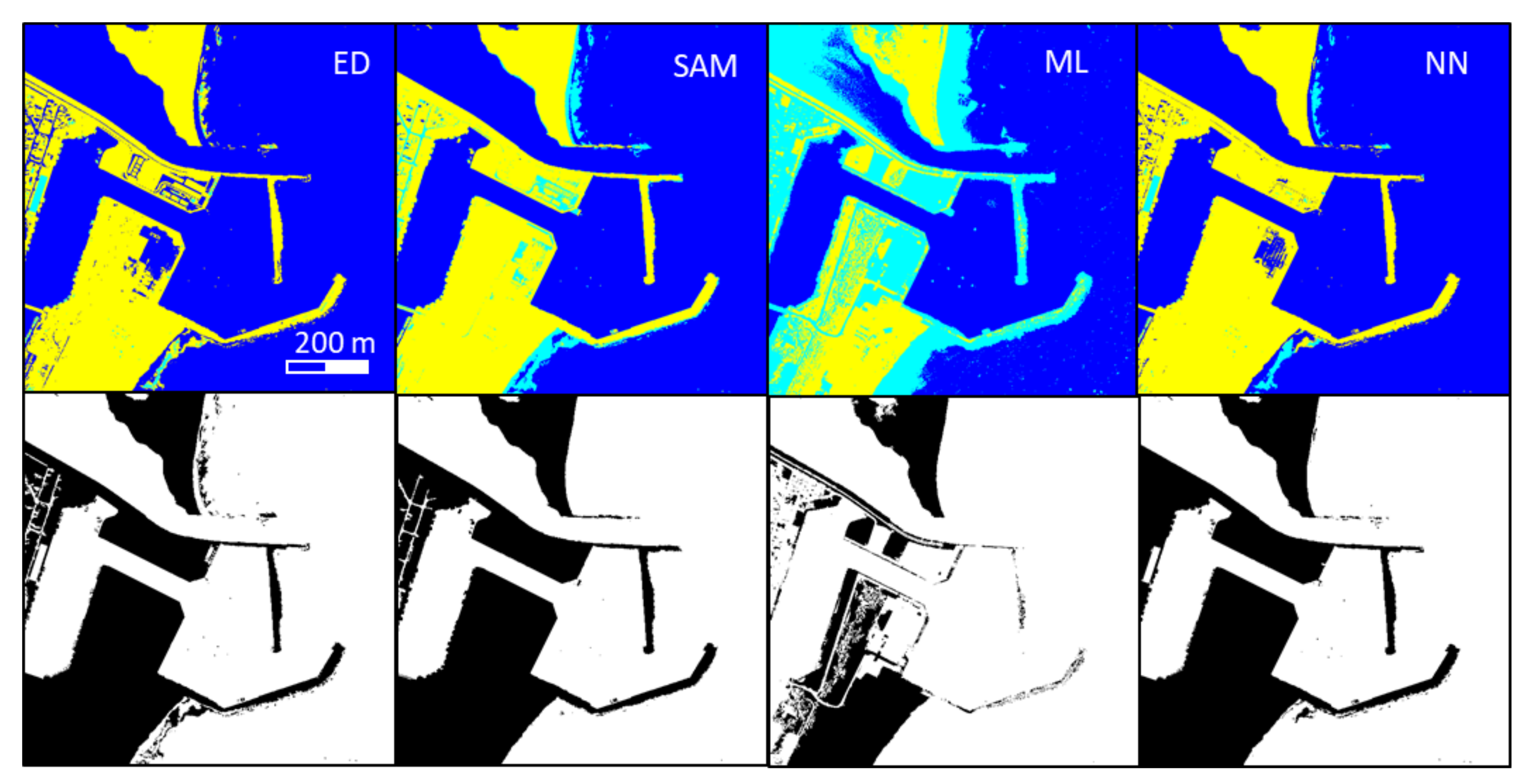
4.1. Comparison of the SVM Method with Other Methods of Classifications
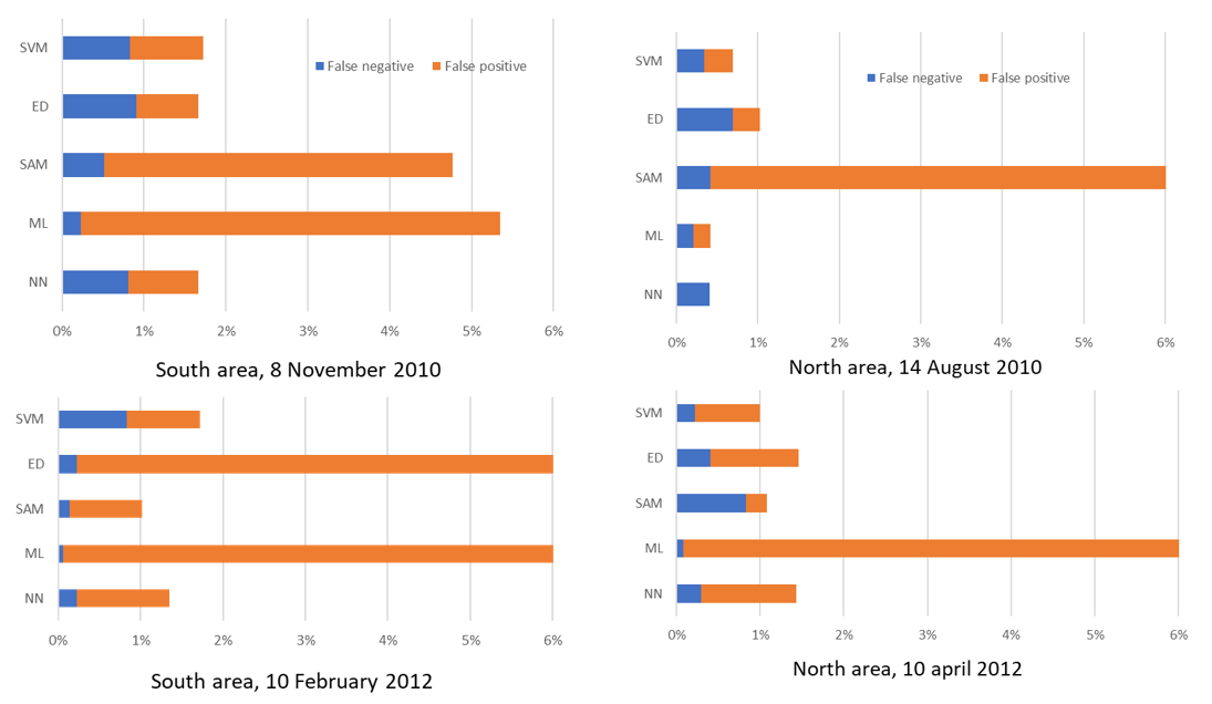
4.2. Comparison of False Positive and False Negative Errors
4.3. Estimation of Erosion and Accretion
5. Conclusions
Author Contributions
Funding
Conflicts of Interest
References
- Small, C.; Nicholls, R.J. A global analysis of human settlement in coastal zones. J. Coast. Res. 2003, 19, 584–599. [Google Scholar]
- Wong, P.P.; Losada, I.J.; Gattuso, J.-P.; Hinkel, J.; Khattabi, A.; McInnes, K.L.; Saito, Y.; Sallenger, A. Coastal systems and low-lying areas. Clim. Chang. 2014, 2104, 361–409. [Google Scholar]
- Blodget, H.; Taylor, P.; Roark, J. Shoreline changes along the Rosetta-Nile Promontory: Monitoring with satellite observations. Mar. Geol. 1991, 99, 67–77. [Google Scholar] [CrossRef]
- Ruiz-Beltran, A.P.; Astorga-Moar, A.; Salles, P.; Appendini, C.M. Short-term shoreline trend detection patterns using SPOT-5 image fusion in the northwest of Yucatan, Mexico. Estuar. Coasts 2019, 42, 1761–1773. [Google Scholar] [CrossRef]
- Collin, A.; Duvat, V.; Pillet, V.; Salvat, B.; James, D. Understanding Interactions between Shoreline Changes and Reef Outer Slope Morphometry on Takapoto Atoll (French Polynesia). J. Coast. Res. 2018, 85, 496–500. [Google Scholar] [CrossRef]
- Hagenaars, G.; de Vries, S.; Luijendijk, A.P.; de Boer, W.P.; Reniers, A.J. On the accuracy of automated shoreline detection derived from satellite imagery: A case study of the sand motor mega-scale nourishment. Coast. Eng. 2018, 133, 113–125. [Google Scholar] [CrossRef]
- Maglione, P.; Parente, C.; Vallario, A. Coastline extraction using high resolution WorldView-2 satellite imagery. Eur. J. Remote Sens. 2014, 47, 685–699. [Google Scholar] [CrossRef]
- Sylla, D.; Minghelli-Roman, A.; Blanc, P.; Mangin, A.; d’Andon, O.H.F. Fusion of multispectral images by extension of the pan-sharpening ARSIS method. IEEE J. Sel. Top. Appl. Earth Obs. Remote Sens. 2014, 7, 1781–1791. [Google Scholar] [CrossRef]
- Chen, W.-W.; Chang, H.-K. Estimation of shoreline position and change from satellite images considering tidal variation. Estuar. Coast. Shelf Sci. 2009, 84, 54–60. [Google Scholar] [CrossRef]
- Wang, H.; Bi, N.; Saito, Y.; Wang, Y.; Sun, X.; Zhang, J.; Yang, Z. Recent changes in sediment delivery by the Huanghe (Yellow River) to the sea: Causes and environmental implications in its estuary. J. Hydrol. 2010, 391, 302–313. [Google Scholar] [CrossRef]
- Kuleli, T.; Guneroglu, A.; Karsli, F.; Dihkan, M. Automatic detection of shoreline change on coastal Ramsar wetlands of Turkey. Ocean Eng. 2011, 38, 1141–1149. [Google Scholar] [CrossRef]
- Pardo-Pascual, J.E.; Almonacid-Caballer, J.; Ruiz, L.A.; Palomar-Vázquez, J. Automatic extraction of shorelines from Landsat TM and ETM+ multi-temporal images with subpixel precision. Remote Sens. Environ. 2012, 123, 1–11. [Google Scholar] [CrossRef] [Green Version]
- Toure, S.; Diop, O.; Kpalma, K.; Maiga, A.S. Shoreline Detection using Optical Remote Sensing: A Review. ISPRS Int. J. Geo Inf. 2019, 8, 75. [Google Scholar] [CrossRef] [Green Version]
- Ghoneim, E.; Mashaly, J.; Gamble, D.; Halls, J.; AbuBakr, M. Nile Delta exhibited a spatial reversal in the rates of shoreline retreat on the Rosetta promontory comparing pre-and post-beach protection. Geomorphology 2015, 228, 1–14. [Google Scholar] [CrossRef]
- Erteza, I.A. An Automatic Coastline Detector for Use with SAR Images; Sandia National Laboratories (SNL-NM): Albuquerque, NM, USA, 1998. [Google Scholar]
- Aedla, R.; Dwarakish, G.; Reddy, D.V. Automatic shoreline detection and change detection analysis of netravati-gurpurrivermouth using histogram equalization and adaptive thresholding techniques. Aquat. Procedia 2015, 4, 563–570. [Google Scholar] [CrossRef]
- Kale, S.; Acarli, D. Shoreline Change Monitoring in Atikhisar Reservoir by Using Remore Sensing and Geographic Information System (GIS). Fresenius Environ. Bull. 2019, 28, 4329. [Google Scholar]
- Mukhopadhyay, A.; Mukherjee, S.; Mukherjee, S.; Ghosh, S.; Hazra, S.; Mitra, D. Automatic shoreline detection and future prediction: A case study on Puri Coast, Bay of Bengal, India. Eur. J. Remote Sens. 2012, 45, 201–213. [Google Scholar] [CrossRef]
- Cao, W.; Zhou, Y.; Li, R.; Li, X. Mapping changes in coastlines and tidal flats in developing islands using the full time series of Landsat images. Remote Sens. Environ. 2020, 239, 111665. [Google Scholar] [CrossRef]
- Vivek, G.; Goswami, S.; Samal, R.; Choudhury, S. Monitoring of Chilika Lake mouth dynamics and quantifying rate of shoreline change using 30 m multi-temporal Landsat data. Data Brief 2019, 22, 595–600. [Google Scholar]
- Pardo-Pascual, J.; Sánchez-García, E.; Almonacid-Caballer, J.; Palomar-Vázquez, J.; de los Santos, E.P.; Fernández-Sarría, A.; Balaguer-Beser, Á. Assessing the accuracy of automatically extracted shorelines on microtidal beaches from Landsat 7, Landsat 8 and Sentinel-2 Imagery. Remote Sens. 2018, 10, 326. [Google Scholar] [CrossRef] [Green Version]
- Liu, Q.; Trinder, J.C.; Turner, I.L. Automatic super-resolution shoreline change monitoring using Landsat archival data: A case study at Narrabeen–Collaroy Beach, Australia. J. Appl. Remote Sens. 2017, 11, 016036. [Google Scholar] [CrossRef]
- Do, A.T.; de Vries, S.; Stive, M.J. The estimation and evaluation of shoreline locations, shoreline-change rates, and coastal volume changes derived from Landsat images. J. Coast. Res. 2019, 35, 56–71. [Google Scholar]
- Sánchez-García, E.; Palomar-Vázquez, J.; Pardo-Pascual, J.; Almonacid-Caballer, J.; Cabezas-Rabadán, C.; Gómez-Pujol, L. An efficient protocol for accurate and massive shoreline definition from mid-resolution satellite imagery. Coast. Eng. 2020, 160, 103732. [Google Scholar] [CrossRef]
- Cabezas-Rabadán, C.; Pardo-Pascual, J.E.; Palomar-Vázquez, J.; Ferreira, Ó.; Costas, S. Satellite Derived Shorelines at an Exposed Meso-tidal Beach. J. Coast. Res. 2020, 95, 1027–1031. [Google Scholar] [CrossRef]
- Yu, L.; Lan, J.; Zeng, Y.; Zou, J. Comparison of Land Cover Types Classification Methods Using Tiangong-2 Multispectral Image. In Proceedings of the Tiangong-2 Remote Sensing Application Conference, Beijing, China, 18 December 2018; Springer: Singapore, 2019; pp. 241–253. [Google Scholar]
- Qin, B.; Li, L.; Li, S. Data Quality Evaluation and Application Potential Analysis of TIANGONG-2 Wide-Band Imaging Spectrometer. Int. Arch. Photogramm. Remote Sens. Spat. Inf. Sci. 2018, 42, 3. [Google Scholar] [CrossRef] [Green Version]
- Kalkan, K.; Bayram, B.; Maktav, D.; Sunar, F. Comparison of support vector machine and object based classification methods for coastline detection. Int. Arch. Photogramm. Remote Sens. Spat. Inf. Sci. 2013, 7, W2. [Google Scholar] [CrossRef] [Green Version]
- Zhang, H.; Jiang, Q.; Xu, J. Coastline Extraction Using Support Vector Machine from Remote Sensing Image. J. Multimed. 2013, 8, 175–182. [Google Scholar]
- Dunbar, P.; McCullough, H.; Mungov, G.; Varner, J.; Stroker, K. Tohoku earthquake and tsunami data available from the national oceanic and atmospheric administration/national geophysical data center. Geomat. Nat. Hazards Risk 2011, 2, 305–323. [Google Scholar] [CrossRef] [Green Version]
- Benz, H.; Ransom, C. USGS Updates Magnitude of Japan’s 2011 Tohoku Earthquake to 9.0; US Geological Survery Website; US Geological Survery: Reston, VA, USA, 2011. [Google Scholar]
- Liu, W.; Yamazaki, F.; Gokon, H.; Koshimura, S. Damage Detection of the 2011 Tohoku, Japan Earthquake from High-resolution SAR Intensity Images. In Proceedings of the 15th World Conference on Earthquake Engineering, Lisbon, Portugal, 24–28 September 2012. [Google Scholar]
- Raby, A.; Macabuag, J.; Pomonis, A.; Wilkinson, S.; Rossetto, T. Implications of the 2011 Great East Japan Tsunami on sea defence design. Int. Disaster Risk Reduct. 2015, 14, 332–346. [Google Scholar] [CrossRef] [Green Version]
- Baba, M. Fukushima accident: What happened? Radiat. Meas. 2013, 55, 17–21. [Google Scholar] [CrossRef]
- Minghelli, A.; Lei, M.; Charmasson, S.; Rey, V.; Chami, M. Monitoring suspended particle matter using GOCI satellite data after the tohoku (Japan) tsunami in 2011. IEEE J. Sel. Top. Appl. Earth Obs. Remote Sens. 2019, 12, 567–576. [Google Scholar] [CrossRef]
- Ambe, D.; Kaeriyama, H.; Shigenobu, Y.; Fujimoto, K.; Ono, T.; Sawada, H.; Saito, H.; Miki, S.; Setou, T.; Morita, T.; et al. Five-minute resolved spatial distribution of radiocesium in sea sediment derived from the Fukushima Dai-ichi Nuclear Power Plant. J. Environ. Radioact. 2014, 138, 264–275. [Google Scholar] [CrossRef] [Green Version]
- Siegel, D.A.; Wang, M.; Maritorena, S.; Robinson, W. Atmospheric Correction of Satellite Ocean Color Imagery: The Black Pixel Assumption. Appl. Opt. 2000, 39, 3582–3591. [Google Scholar] [CrossRef]
- Lee, Z.; Carder, K.L.; Mobley, C.D.; Steward, R.G.; Patch, J.S. Hyperspectral remote sensing for shallow Waters. I. A semianalytical model. Appl. Opt. 1998, 37, 6329–6338. [Google Scholar] [CrossRef]
- Lee, Z.; Lubac, B.; Werdell, J.; Armone, R. An update of the quasi-analytical algorithm (QAA_v5). Int. Ocean Color Group Softw. Rep. 2009, 1–9. [Google Scholar]
- Gerbermann, A.; Neher, D. Reflectance of varying mixtures of a clay soil and sand. Photogramm. Eng. Remote Sens. 1979, 45, 1145–1151. [Google Scholar]
- Kokhanovsky, A. Spectral reflectance of whitecaps. J. Geophys. Res. Ocean. 2004, 109, C05021. [Google Scholar] [CrossRef]
- Foody, G.M.; Mathur, A. Toward intelligent training of supervised image classifications: Directing training data acquisition for SVM classification. Remote Sens. Environ. 2004, 93, 107–117. [Google Scholar] [CrossRef]
- Imakiire, T.; Koarai, M. Wide-area land subsidence caused by “the 2011 off the Pacific Coast of Tohoku Earthquake”. Soils Found. 2012, 52, 842–855. [Google Scholar] [CrossRef] [Green Version]
- Tsuruta, T.; Harada, H.; Misonou, T.; Matsuoka, T.; Hodotsuka, Y. Horizontal and vertical distributions of 137 Cs in seabed sediments around the river mouth near Fukushima Daiichi Nuclear Power Plant. J. Oceanogr. 2017, 73, 547–558. [Google Scholar] [CrossRef] [Green Version]
- Richards, J.; Jia, X. Remote Sensing Digital Image Analysis-Hardback; Springer: Berlin/Heidelberg, Germany, 2006. [Google Scholar]
- Wang, L.; Silván-Cárdenas, J.L.; Sousa, W.P. Neural network classification of mangrove species from multi-seasonal Ikonos imagery. Photogramm. Eng. Remote Sens. 2008, 74, 921–927. [Google Scholar] [CrossRef]
- Gomez, C.; Wulder, M.A.; Dawson, A.G.; Ritchie, W.; Green, D.R. Shoreline change and coastal vulnerability characterization with Landsat imagery: A case study in the Outer Hebrides, Scotland. Scott. Geogr. J. 2014, 130, 279–299. [Google Scholar] [CrossRef]
- Dingerson, L.M. Predicting Future Shoreline Condition Based on Land Use Trends, Logistic Regression, and Fuzzy Logic. Master’s Thesis, College of William and Mary, Williamsburg, VA, USA, 2005. [Google Scholar]
- Kench, P.; Nichol, S.; Smithers, S.; McLean, R.; Brander, R. Tsunami as agents of geomorphic change in mid-ocean reef islands. Geomorphology 2008, 95, 361–383. [Google Scholar] [CrossRef]
- Kumar, P.; Gupta, D.K.; Mishra, V.N.; Prasad, R. Comparison of support vector machine, artificial neural network, and spectral angle mapper algorithms for crop classification using LISS IV data. Int. J. Remote Sens. 2015, 36, 1604–1617. [Google Scholar] [CrossRef]
- Nitze, I.; Schulthess, U.; Asche, H. Comparison of machine learning algorithms random forest, artificial neural network and support vector machine to maximum likelihood for supervised crop type classification. In Proceedings of the 4th International Conference on GEographic Object Based Image Analysis, Rio de Janeiro, Brazil, 7–9 May 2012; p. 35. [Google Scholar]


| Date of Acquisition of WV-2 Images | False Positive Error (%) | False Negative Error (%) | |
|---|---|---|---|
| 2 Classes/3 Classes | 2 Classes/ 3 Classes | ||
| Southern site | 08 Nov. 2010 | 0.88/0.83 | 1.54/0.89 |
| 10 Feb. 2012 | 0.69/0.68 | 0.30/0.19 | |
| Northern site | 4 Aug. 2010 | 0.92/0.59 | 1.67/0.34 |
| 10 Apr. 2012 | 0.86/0.78 | 0.78/0.22 |
| Erosion (m2/km) of Coast) | Accretion (m2/km of Coast) | ESRE on Erosion | ESRE on Accretion | ||
|---|---|---|---|---|---|
| Southern site (25 km of coast) | Reference values | 16.5 | 6.9 | ||
| SVM2 SVM3 | 48.3 19.7 | 1.10 8.6 | 192% 19% | −84% 24% | |
| Northern site (19 km of coast) | Reference values | 29.1 | 27.3 | ||
| SVM2 SVM3 | 58.2 28.6 | 69.1 30.7 | 100% −2% | 153% 13% |
| Erosion (m2/km) | Accretion (m2/km) | ESRE on Erosion | ESRE on Accretion | ||
|---|---|---|---|---|---|
| Southern site (25 km of coast) | Reference values | 16.5 | 6.9 | ||
| ED | 104.1 | 8.5 | 529% | 22% | |
| SAM | 9.4 | 64.7 | −43% | 834% | |
| ML | 1119.5 | 35.8 | 6671% | 416% | |
| SVM | 19.7 | 8.6 | 19% | 24% | |
| NN | 23.9 | 4.5 | 45% | −35% | |
| Northern site (19 km of coast) | Reference values | 29.1 | 27.3 | ||
| ED | 25.1 | 62.4 | −14% | 129% | |
| SAM | 39.0 | 22.7 | 34% | −17% | |
| ML | 64.7 | 1644.5 | 123% | 5926% | |
| SVM | 28.6 | 30.7 | −2% | 13% | |
| NN | 41.7 | 31.8 | 43% | 16% |
© 2020 by the authors. Licensee MDPI, Basel, Switzerland. This article is an open access article distributed under the terms and conditions of the Creative Commons Attribution (CC BY) license (http://creativecommons.org/licenses/by/4.0/).
Share and Cite
Minghelli, A.; Spagnoli, J.; Lei, M.; Chami, M.; Charmasson, S. Shoreline Extraction from WorldView2 Satellite Data in the Presence of Foam Pixels Using Multispectral Classification Method. Remote Sens. 2020, 12, 2664. https://0-doi-org.brum.beds.ac.uk/10.3390/rs12162664
Minghelli A, Spagnoli J, Lei M, Chami M, Charmasson S. Shoreline Extraction from WorldView2 Satellite Data in the Presence of Foam Pixels Using Multispectral Classification Method. Remote Sensing. 2020; 12(16):2664. https://0-doi-org.brum.beds.ac.uk/10.3390/rs12162664
Chicago/Turabian StyleMinghelli, Audrey, Jérôme Spagnoli, Manchun Lei, Malik Chami, and Sabine Charmasson. 2020. "Shoreline Extraction from WorldView2 Satellite Data in the Presence of Foam Pixels Using Multispectral Classification Method" Remote Sensing 12, no. 16: 2664. https://0-doi-org.brum.beds.ac.uk/10.3390/rs12162664