ISAR Image Matching and Three-Dimensional Scattering Imaging Based on Extracted Dominant Scatterers

Abstract

This paper studies inverse synthetic aperture radar (ISAR) image matching and three-dimensional (3D) scattering imaging based on extracted dominant scatterers. In the condition of a long baseline between two radars, it is easy for obvious rotation, scale, distortion, and shift to occur between two-dimensional (2D) radar images. These problems lead to the difficulty of radar-image matching, which cannot be resolved by motion compensation and cross-correlation. What is more, due to the anisotropy, existing image-matching algorithms, such as scale invariant feature transform (SIFT), do not adapt to ISAR images very well. In addition, the angle between the target rotation axis and the radar line of sight (LOS) cannot be neglected. If so, the calibration result will be smaller than the real projection size. Furthermore, this angle cannot be estimated by monostatic radar. Therefore, instead of matching image by image, this paper proposes a novel ISAR imaging matching and 3D imaging based on extracted scatterers to deal with these issues. First, taking advantage of ISAR image sparsity, radar images are converted into scattering point sets. Then, a coarse scatterer matching based on the random sampling consistency algorithm (RANSAC) is performed. The scatterer height and accurate affine transformation parameters are estimated iteratively. Based on matched scatterers, information such as the angle and 3D image can be obtained. Finally, experiments based on the electromagnetic simulation software CADFEKO have been conducted to demonstrate the effectiveness of the proposed algorithm.

1. Introduction

Inverse synthetic aperture radar (ISAR) imaging, especially two-dimensional (2D) imaging, has been extensively used in civil and military applications because of its capability to generate high-resolution images of noncooperative targets. There are many methods of 2D imaging, including noise suppression, sparse imaging, motion compensation, and so on [1,2,3,4,5,6,7,8,9,10,11,12]. A 2D image is the projection of a three-dimensional (3D) target on the range-Doppler (RD) plane [6,7,8,9,10,11,12,13,14,15,16,17,18,19,20,21,22,23,24,25,26,27]. However, 2D imaging has several unavoidable shortcomings. For example, the azimuth dimension of the 2D image just reflects the Doppler distribution of every scattering point. What is more, most calibration algorithms achieve calibration by estimating the target rotation angle during the observation time [13,14]. These algorithms assume the target rotation axis is orthogonal to the radar line of sight (LOS). However, in practical applications, meeting the requirements of complete orthogonality is not an easy matter because of the noncooperative targets. The information derived from a 3D image is more than that derived from a 2D image. Therefore, the study of 3D imaging has received significant attention in recent years [15,16,17,18,19,20,21,22,23,24,25,26,27,28,29,30,31,32,33,34,35]. The existing 3D imaging methods can be roughly categorized into two groups, corresponding to monostatic and multistatic radar systems.

3D imaging methods via monostatic radar include 3D matched filtering [15,16], which is a direct extension of 2D imaging, and 3D reconstruction based on ISAR image sequences [17,18,19,20,21,22]. It is worth noting that 3D imaging with multipass SAR data is excluded [23]. Generally, when the target spinning axis is not perpendicular to the LOS, 3D imaging can be performed by 3D matched filtering. The accuracy of the third dimension is determined by the sampling frequency in the third dimension. Moreover, the methods of 3D reconstruction based on the ISAR image sequence need accurate scattering point extraction, scattering point trace association, and scattering point trace matrix decomposition. 3D reconstruction based on sequencing also requires a large rotation angle. What is more, accurate scatter extraction and association are necessary to generate an accurate trajectory matrix, which is the foundation for high-resolution 3D reconstruction. It should be noted that these algorithms are time-consuming, and the number of ISAR image sequences is large.

3D imaging methods via multistation include Interferometric ISAR (InISAR) and 3D imaging via distributed radar network. InISAR generally employs three antennas that need to be properly designed [24,25,26,27,28,29,30,31,32,33,34,35]. Because InISAR gets a 3D image by phase difference, the baselines between the three antennas are a few meters. Images from the three antennas are basically the same. Although the InISAR system can easily obtain 3D images without prior knowledge of the target motion, it is of relatively high cost and hardware complexity compared with 3D imaging via monostatic radar or distributed radar network. On the contrary, distributed radar can make full use of existing radars for 3D imaging and other applications.

This paper studies ISAR image matching and 3D scattering imaging based on extracted dominant scatterers. Unlike InISAR, the proposed algorithm gets a 3D image by the difference of the scatterer’s position from two arbitrary radars. Therefore, a long baseline is more conducive to high-precision 3D imaging for the proposed method. However, when the baseline is too long, image rotation, scale, distortion, and obvious anisotropy will occur, which are not conducive to radar image matching. Therefore, the optimal baseline is to make the two radar images rotate and distortion, but the anisotropy is not obvious. Meanwhile, 2D imaging strongly depends on the RD plane. Therefore, ISAR images from different RD planes vary dramatically.

These problems are a challenge for ISAR image matching. Improved optical image matching algorithms [36], such as the modified scale invariant feature transform (SIFT) and Harris algorithms, are suitable for theoretically simulated radar images, but not for real ISAR images. Due to different imaging mechanisms, the magnitude of the scattering point from a real ISAR image is not the same as the optic picture. What is more, these problems cannot be solved by motion compensation and cross-correlation on ISAR images. To solve the above problems, the proposed method adopts the image matching based on extracted dominant scatterers, which is different from the image-based SIFT. This method can make full use of existing radars to derive the target 3D image. First, for the sparsity of the ISAR image, the radar images are transformed into scattering point sets by scattering center extraction [37]. Then, a coarse scatterer matching based on the random sampling consistency algorithm (RANSAC) is performed. The scatterer height and accurate affine transformation parameters are estimated iteratively to obtain fine scatterer matching. Based on matched scatterers, information such as the 3D image and the angle between the LOS and the target rotation axis can be obtained. Finally, experiments based on the electromagnetic simulation software CADFEKO have been conducted to demonstrate the effectiveness of the proposed algorithm.

This paper is organized as follows. In Section 2, the radar system and the signal model are established. In Section 3, by extracting scattering centers, two scattering point sets can be obtained. After RANSAC, a coarse scatterer matching is achieved. Then, an automatic iteration process based on affine transformation can be performed to achieve accurate scattering point set matching. Meanwhile, the scattering point height and the angle between the target spinning axis and LOS can be obtained. In Section 4, experiments based on two simulation datasets, using the electromagnetic simulation software CADFEKO, are performed to demonstrate the effectiveness of the proposed algorithm.

2. Signal Model

A radar system with two arbitrary configuration radars locating at $A$ and $B$ is depicted in Figure 1a, where the radar coordinate system $O_0-X_0{Y}_0{Z}_0$, the transition coordinate system $O-X_1{Y}_1{Z}_1$, and the target coordinate system $O-XYZ$ are established. For ease of description and analysis, these three reference coordinate systems are marked as $S_0$, $S_1$, and $S$, respectively. Having to deal with these three coordinate systems, we denote scattering points in 3D space by using a subscript according to the specific reference, e.g., $P_{s_1}$ and $P_{s_0}$ are the same point expressed with the reference system coordinates $S_0$ and $S_1$, respectively.

The reference system $S_0$ is embedded in radar A and centered in $O_0$. The $X_0$-axis is aligned with the LOS of radar A. Radar B is located in the plane $(X_0,Y_0)$. The reference system $S$ is embedded in the target and centered in $O$. In practical conditions, external forces on the target produce angular motions that are represented by the angular rotation vector $\mathsf{\Omega }$, which is aligned with the $Z$-axis. Its projection onto the plane orthogonal to LOS of radar A defines the effective rotation component ${\mathsf{\Omega }}_{eff}$, which forms the $Z_1$-axis. The plane $(Y_1,X_1)$ is the imaging plane, whose axes correspond to range and the cross-range dimensions. For an easier understanding, the radar coordinate system and target rotation axis are abstractly represented in Figure 1b. $\alpha$ is the angle between the target rotation axis and $X_0$-axis, marked as ARX, which can influence the projection and calibration results. $\beta$ is the angle between the target rotation axis and the $Y_0$-axis, marked as ARY. Without loss of generality, we assume that the $X_1$-axis is aligned with $X_0$-axis and the $Y$-axis is aligned with $Y_1$-axis. According to right-handed coordinates, the $Z_0$-axis and the $X$-axis can be derived.

Moreover, we consider the target as a rigid body moving toward the $Z$-axis concerning system $S$. The target is composed of point-like scatterers, and the position of scatterer $P$ with respect to $S$ is

$$P_S=\left[\begin{array}{l}x\cos (\mathsf{\Omega }{t}_m)-y\sin (\mathsf{\Omega }{t}_m)\\ x\sin (\mathsf{\Omega }{t}_m)+y\cos (\mathsf{\Omega }{t}_m)\\ z+v{t}_m\end{array}\right]$$

(1)

where $\mathsf{\Omega }=\left|\mathsf{\Omega }\right|$, and $t_m$ denotes slow time. The angle between the $Z$-axis and the $Z_0$-axis is $\theta$, which can be derived as

$$\cos \theta =\pm \sqrt{1-{\cos }^2\alpha -{\cos }^2\beta }$$

(2)

where the $Z_1$-axis is the projection result of the $Z$-axis on the plane $(Y_0,Z_0)$, $\cos \theta =\sqrt{1-{\cos }^2\alpha -{\cos }^2\beta }$. The angular rotation vector $\mathsf{\Omega }$ with the radar coordinate system can be expressed as

$$Z_{S_0}=[\cos \alpha ,\cos \beta ,\cos \theta ]$$

(3)

Concerning the transition coordinate system, the target coordinate system is represented as

$$X_{S_1}=[\sin \alpha ,0,-\cos \alpha ]$$

(4)

$$Y_{S_1}=[0,1,0]$$

(5)

$$Z_{S_1}=[\cos \alpha ,0,\sin \alpha ]$$

(6)

With respect to the radar coordinate system, the transition coordinate system is represented as

$$X_{1,S_0}=[1,0,0]$$

(7)

$$Y_{1,S_0}=\frac{X_0\times Z_{S_0}}{\Vert X_0\times Z_{S_0}\Vert }$$

(8)

$$Z_{1,S_0}=\frac{X_0\times Y_{1,S_0}}{\Vert X_0\times Y_{1,S_0}\Vert }$$

(9)

The relationship between these three coordinate systems can be formulated as

$$S_1=S_0{C}_1$$

(10)

$$S=S_{1}C$$

(11)

where $C=\left[X_{S_1}{}^T,Y_{S_1}{}^T,Z_{S_1}{}^T\right]$, $C_1=\left[X_{1,S_0}{}^T,Y_{1,S_0}{}^T,Z_{1,S_0}{}^T\right]$.

Therefore, the transformation from the target coordinate system into the radar coordinate system can be formulated as

$$P_{S_0}=\left[R_0,0,0\right]+C_{1}C{P}_S=\left[R_0+{\xi }_1,{\xi }_2,{\xi }_3\right]$$

(12)

where ${\cos }^2\beta <{\sin }^2\alpha ,\alpha \in \left(0,\pi /2\right)$, and ${\xi }_i,i=1,2,3$ can be expressed as

$${\xi }_1=\sin \alpha \left(x\cos (w{t}_m)-y\sin (w{t}_m)\right)+z\cos \alpha +v{t}_m\cos \alpha$$

(13)

$${\xi }_2=\frac{\cos \alpha }{\sin \alpha }\cos \beta \left(x\cos (w{t}_m)-y\sin (w{t}_m)\right)-\frac{\cos \theta }{\sin \alpha }\left(x\sin (w{t}_m)+y\cos (w{t}_m)\right)-\left(z+v{t}_m\right)\cos \beta$$

(14)

$${\xi }_3=\frac{\cos \alpha \cos \theta }{\sin \alpha }\left(x\cos (w{t}_m)-y\sin (w{t}_m)\right)+\frac{\cos \beta }{\sin \alpha }\left(x\sin (w{t}_m)+y\cos (w{t}_m)\right)-\left(z+v{t}_m\right)\cos \theta$$

(15)

According to Figure 1, the location of radar A can be expressed as $D_{A,S_0}=[0,0,0]$. The distance from radar A to scattering point $P$ can be expressed by

$$R_{A,P}\left(t_m\right)=\Vert P_S-D_{A,S_0}{}^T\Vert ={\left({\left({\xi }_1+R_0\right)}^2+{\xi }_2{}^2+{\xi }_3{}^2\right)}^{1/2}$$

(16)

The first-order Taylor expansion of (16) is carried out, and (16) can be rewritten as

$$R_{A,P}\left(t_m\right)=R_0+{\xi }_1+\frac{{\xi }_1{}^2+{\xi }_2{}^2+{\xi }_3{}^2}{2R_0}$$

(17)

Substituting $\left(x,y,z\right)$ into (14), (17) can be rewritten as

$$R_{A,P}\left(t_m\right)=x\sin \alpha \cos (w{t}_m)-y\sin \alpha \sin (w{t}_m)+z\cos \alpha +R_0+v{t}_m\cos \alpha +\frac{{\xi }_1{}^2+{\xi }_2{}^2+{\xi }_3{}^2}{2R_0}$$

(18)

The location of radar B can be expressed as follows:

$$D_{B,S_0}=[R_0-R_r\cos \phi ,R_r\sin \phi ,0]$$

(19)

The distance from scattering point $P$ to radar B is $R_{B,P}\left(t_m\right)$, which can be expressed as

$$R_{B,P}\left(t_m\right)=\Vert P_S-D_{B,S_0}{}^T\Vert \approx R_r+{\xi }_1\cos \varphi -{\xi }_2\sin \varphi +\frac{{\xi }_1{}^2+{\xi }_2{}^2+{\xi }_3{}^2}{2R_r}$$

(20)

Suppose that the pulse of the linear frequency modulated signal at a pulse repetition frequency of $PRF$ is transmitted by radar A. After preprocessing, including de-modulation to the baseband and range compression, the processed echo data of scattering point $P$ can be expressed as

$$S_{i,p}(t,t_m)={\sigma }_p\cdot \sin \mathrm{c}\left(W\left(t-\frac{2R_{i,p}\left(t_m\right)}{c}\right)\right)\cdot \exp \left(-j4\pi f_c\frac{R_{i,p}\left(t_m\right)}{c}\right)$$

(21)

where $i=A,B$ is the radar index, ${\sigma }_p$ is the complex scattering coefficient of scattering point $P$, $t$ is the fast time in the range dimension, $f_c$ is the center frequency of the transmitted signal, $c$ is the transmitting velocity of the electromagnetic wave, and $W$ is the spectrum bandwidth of the transmitted signal.

3. Theory and Method

The proposed method is shown in Figure 2. After receiving the target echoes from two arbitrary radars, motion compensation was accomplished first. Then, through scattering point extraction, the ISAR image was converted into a scatterer set.

The process in the yellow rectangle was used to match scattering point sets and 3D imaging. First, the height of each scatterer was set as one. Meanwhile, a coarse scatterer matching in RANSAC was carried out. Based on the preliminary transformation, one could estimate ARX and ARY. Then, the scatterer height was obtained based on the preliminary ARX and ARY. After scatterer height estimation, affine transformation with estimated scatterer height was performed. The estimation of ARX, ARY, and scatterer height was executed iteratively. The iteration was stopped when the estimation of ARX and ARY varied slightly. Finally, an accurate ARX and ARY was derived from a small range of searching. The operations in the red rectangle will be described in detail in the rest of this section.

3.1. Scattering Point Sets Matching based on RANSAC and Affine Transformation

After motion compensation, the images from radar A and radar B can be expressed as

$$I_i\left(t,f_a\right)={\sigma }_i\sin \mathrm{c}\left(W\left(t-2\frac{x_i}{c}\right)\right)\cdot \sin \mathrm{c}\left(\frac{1}{PRF}\left(f_a+y_i\frac{\omega }{2\pi }\right)\right)\exp (-j{\phi }_i)$$

(22)

where $i=A,B$, ${\phi }_i$ denotes the corresponding radar residual phase, and $x_i$ and $y_i$ denote scattering location in the corresponding image $i$. For a short observation time, $\cos (w{t}_m)$ can be approximated as 1, and $\sin (w{t}_m)$ can be approximated as $w{t}_m$. After scattering point extraction, two scattering point sets can be achieved: scattering point set A $\left(x_A,y_A\right)$ with $N_A$ scatterers and scattering point set B $\left(x_B,y_B\right)$ with $N_B$ scatterers. For the convenience of expression, $\left(x_A,y_A\right)$ and $\left(x_B,y_B\right)$ are defined as SPA and SPB, respectively. According to (16) to (22), SPA can be expressed as

$$x_A=x\sin \alpha +z\cos \alpha$$

(23)

$$y_A=-y\sin \alpha$$

(24)

Similarly, SPB can be expressed as

$$x_B=x_A\cos \phi -x_A\frac{\cos \alpha }{{\sin }^2\alpha }\sin \phi \cos \beta -y_A\frac{\cos \theta }{{\sin }^2\alpha }\sin \phi +z\cos \beta \sin \phi \left(1+{\cot }^2\alpha \right)$$

(25)

$$y_B=x_A\frac{\cos \theta }{{\sin }^2\alpha }\sin \phi +y_A\cos \phi -y_A\frac{\cos \alpha }{{\sin }^2\alpha }\sin \phi \cos \beta -z\cos \alpha \sin \phi \frac{\cos \theta }{{\sin }^2\alpha }$$

(26)

Therefore, the relationship between SPA and SPB can be achieved by

$$\left[\begin{array}{c}{x}_B\\ y_B\\ z\end{array}\right]=U\left[\begin{array}{c}{x}_A\\ y_A\\ z\end{array}\right]=\left[\begin{array}{ccc}{u}_1& u_2& u_3\\ u_4& u_5& u_6\\ 0& 0& 1\end{array}\right]\left[\begin{array}{c}{x}_A\\ y_A\\ z\end{array}\right]$$

(27)

where $U\in R^{3\times 3}$, the element of $U$ is $u_i,i=1,2,...,6$, $u_1=\cos \phi -\cos \alpha /{\sin }^2\alpha \cos \beta \sin \phi$, $u_2=-\sin \phi \cos \theta /{\sin }^2\alpha$, $u_3=\cos \beta \sin \phi \left(1+{\cot }^2\alpha \right)$, $u_4=-u_2$, $u_5=u_1$, and $u_6=-\cos \alpha \sin \phi \cos \theta /{\sin }^2\alpha$.

Through the analysis of (27), one can find that angles $\alpha ,\beta ,\phi$ can cause rotation, scaling, and shift for image B. Because $u_5=u_1$, the scaling in the range and azimuth dimensions is the same. Furthermore, $z$ for each scattering point is different. This means, for range and azimuth dimensions, each scattering point has a different shift. Therefore, compared with image A, rotation, scaling, and shift appeared in image B. In order to estimate preliminary ARX and ARY, assume that $z$ of all the scatterers is one at the start time. According to RANSAC, assume the total estimation number is $K$. In the $k$th estimation, three pairs of scatterers are chosen randomly to form an affine transformation, expressed as

$$\left[\begin{array}{c}{x}_{B_1}\\ x_{B_2}\\ x_{B_3}\\ y_{B_1}\\ y_{B_2}\\ y_{B_3}\end{array}\right]=\left[\begin{array}{cccccc}{x}_{A_1}& y_{A_1}& 1& 0& 0& 0\\ x_{A_2}& y_{A_2}& 1& 0& 0& 0\\ x_{A_3}& y_{A_3}& 1& 0& 0& 0\\ 0& 0& 0& x_{A_1}& y_{A_1}& 1\\ 0& 0& 0& x_{A_2}& y_{A_2}& 1\\ 0& 0& 0& x_{A_3}& y_{A_3}& 1\end{array}\right]\left[\begin{array}{c}{u}_1\\ u_2\\ u_3\\ u_4\\ u_5\\ u_6\end{array}\right]$$

(28)

By solving (28), $U_k$ is estimated. The converted SPA $(x_B{}^{\prime },y_B{}^{\prime })$ can be obtained by

$$\left[\begin{array}{c}{x}_B{}^{\prime }\\ y_B{}^{\prime }\\ 1\end{array}\right]=U_k\left[\begin{array}{c}{x}_A\\ y_A\\ 1\end{array}\right]$$

(29)

Scatterer matching can be performed based on the minimum Euclidean distance between the converted SPA and SPB. For the $i\mathrm{th}$ scattering point in image A, the matched scattering point can be expressed as

$$j_i=\underset{j}{\min }\left(\sqrt{{\left(x_{B_i}{}^{\prime }-x_{Bj}\right)}^2+{\left(y_{Bi}{}^{\prime }-y_{Bj}\right)}^2}\right)$$

(30)

where $i$ and $j$ are the index of scattering point in image A and image B, respectively. $j_i$ is the matched scattering point index. Assume the number of matched scatterers is $N_k$. Then, the preliminary scatterer matching result is

$$\begin{array}{l}\{\begin{array}{c}U=U_d\\ N=N_d\end{array}\\ s.t.\begin{array}{c}\end{array}d=\underset{k}{\max }{N}_k\end{array}$$

(31)

3.2. Estimation of ARX and ARY

After the process of RANSAC, the rough relationship $U$ between the scattering point set can be obtained. To estimate ARX and ARY from $U$, we let

$$k_1=\frac{\cos \phi -u_1}{\sin \phi }=\frac{\cos \alpha }{{\sin }^2\alpha }\cos \beta$$

(32)

$$k_2=\frac{u_2}{\sin \phi }=-\frac{\sqrt{{\sin }^2\alpha -{\cos }^2\beta }}{{\sin }^2\alpha }$$

(33)

Combining (32) and (33), we have

$$\sin \alpha =\sqrt{\frac{\left(k_2{}^2+k_1{}^2+1\right)\pm \sqrt{{\left(k_2{}^2+k_1{}^2+1\right)}^2-4k_2{}^2}}{2k_2{}^2}}$$

(34)

$$\cos \beta =k_1\frac{{\sin }^2\alpha }{\cos \alpha }$$

(35)

Due to the limitation that $\sin \alpha$ is less than 1, then (34) can be expressed as

$$\sin \alpha =\sqrt{\frac{\left(k_2{}^2+k_1{}^2+1\right)-\sqrt{{\left(k_2{}^2+k_1{}^2+1\right)}^2-4k_2{}^2}}{2k_2{}^2}}$$

(36)

Therefore, ARX and ARY can be derived by

$$\alpha =\mathrm{asin}\left(\sqrt{\frac{\left(k_2{}^2+k_1{}^2+1\right)-\sqrt{{\left(k_2{}^2+k_1{}^2+1\right)}^2-4k_2{}^2}}{2k_2{}^2}}\right)$$

(37)

$$\beta =\mathrm{acos}\left(k_1\frac{{\sin }^2\alpha }{\cos \alpha }\right)$$

(38)

Therefore, we let

$$k_3=\frac{\cos \phi -u_5}{\sin \phi }=\frac{\cos \alpha }{{\sin }^2\alpha }\cos \beta$$

(39)

$$k_4=\frac{u_4}{\sin \phi }=\frac{\sqrt{{\sin }^2\alpha -{\cos }^2\beta }}{{\sin }^2\alpha }$$

(40)

The final estimation of ARX and ARY can be expressed as

$$\alpha =\mathrm{asin}\left(\mathrm{mean}\left(\begin{array}{l}\sqrt{\frac{\left(k_2{}^2+k_1{}^2+1\right)-\sqrt{{\left(k_2{}^2+k_1{}^2+1\right)}^2-4k_2{}^2}}{2k_2{}^2}},\\ \sqrt{\frac{\left(k_4{}^2+k_3{}^2+1\right)-\sqrt{{\left(k_4{}^2+k_3{}^2+1\right)}^2-4k_4{}^2}}{2k_4{}^2}}\end{array}\right)\right)$$

(41)

$$\beta =\mathrm{acos}\left(\mathrm{mean}\left(k_1\frac{{\sin }^2\alpha }{\cos \alpha },k_3\frac{{\sin }^2\alpha }{\cos \alpha }\right)\right)$$

(42)

3.3. Estimation of Scatterer Height and Affine Transformation Considering Scatterer Height

The difference of each scatterer can be represented as

$$\left[\begin{array}{c}\mathsf{\Delta }{x}_{B{j}_i}\\ \mathsf{\Delta }{y}_{B{j}_i}\end{array}\right]=\left[\begin{array}{c}{x}_{B{j}_i}\\ y_{B{j}_i}\end{array}\right]-\left[\begin{array}{cc}{u}_1& u_2\\ u_4& u_5\end{array}\right]\left[\begin{array}{c}{x}_{Ai}\\ y_{Ai}\end{array}\right]$$

(43)

According to (25) and (26), the different shift can be rewritten by

$$\left[\begin{array}{c}\mathsf{\Delta }{x}_{B{j}_i}\\ \mathsf{\Delta }{y}_{B{j}_i}\end{array}\right]=z\left[\begin{array}{c}\cos \beta \sin \phi \left(1+{\cot }^2\alpha \right)\\ -\cos \alpha \sin \phi \frac{\sqrt{{\sin }^2\alpha -{\cos }^2\beta }}{{\sin }^2\alpha }\end{array}\right]$$

(44)

Substituting $\alpha$ and $\beta$ into (25) and (26), the estimated target height can be expressed as

$$z=\left[\begin{array}{c}\mathsf{\Delta }{x}_{B{j}_i}\\ \mathsf{\Delta }{y}_{B{j}_i}\end{array}\right]{\left[\begin{array}{c}\cos \beta \sin \phi \left(1+{\cot }^2\alpha \right)\\ -\cos \alpha \sin \phi \frac{\sqrt{{\sin }^2\alpha -{\cos }^2\beta }}{{\sin }^2\alpha }\end{array}\right]}^{-1}$$

(45)

Combining with the estimated $z$, the relationship between SPA and SPB can be rewritten as

$$\left[\begin{array}{c}{x}_{B_1}\\ ⋮\\ x_{B_N}\\ y_{B_1}\\ ⋮\\ y_{B_N}\end{array}\right]=\left[\begin{array}{cccccc}{x}_{A_1}& y_{A_1}& z_1& 0& 0& 0\\ ⋮& ⋮& ⋮& 0& 0& 0\\ x_{A_N}& y_{A_N}& z_{{}_N}& 0& 0& 0\\ 0& 0& 0& x_{A_1}& y_{A_1}& z_1\\ 0& 0& 0& ⋮& ⋮& ⋮\\ 0& 0& 0& x_{A_{{}_N}}& y_{A_{{}_N}}& z_{{}_N}\end{array}\right]\left[\begin{array}{c}{u}_1\\ u_2\\ u_3\\ u_4\\ u_5\\ u_6\end{array}\right]$$

(46)

Then, (46) can be rewritten as

$$b=A\mu$$

(47)

where $b={\left[x_{B_1},\cdots ,x_{B_{Nd}},y_{B_1},\cdots ,y_{B_{Nd}}\right]}^T$, $\mu ={[u_1,u_2,u_3,u_4,u_5,u_6]}^T$, and $A$ is the middle part of (31). After QR decomposition, $A$ can be expressed as

$$A=QR$$

(48)

Because $Q$ is an orthogonal matrix, then $Q{Q}^T=I$, where $I$ is a unit matrix, ${(•)}^T$ denotes transpose, and $R$ denotes the upper triangular matrix. After computing, $\mu$ can be derived by

$$\mu =R\backslash Q^{T}b$$

(49)

Based on the above analysis, the recalibration of the range and azimuth dimensions can be expressed as

$$x=\frac{x_A-z\cos \alpha }{\sin \alpha }$$

(50)

$$y=-\frac{y_A}{\sin \alpha }$$

(51)

Combining with the estimated $z$, the target 3D scattering image $\left(x,y,z\right)$ is obtained.

4. Simulations

In this section, to demonstrate the effectiveness and superiority of the proposed algorithm, some experiments based on two different simulation datasets are conducted. To verify the capability of the proposed method, the first experiment compared the modified SIFT algorithm from [36] and the proposed method based on point scattering center theory. Because real data are hard to obtain, a second experiment was conducted based on CADFEKO software, by which the simulated echo was similar to the real one. For these two experiments, the radar parameters were the same. The radar operated in the Ku-band. The signal bandwidth was 2 GHz.

4.1. Experiment on Point Scattering Simulation Data

To compare the modified SIFT with the proposed method, a point simulated satellite was used. The system parameters are listed below in

Table 1. Parameter settings.

Parameters	ARX	ARY	Bistatic Angle	Dominant Scatter
Setting value	60.00°	45°	20°	212

. Figure 3 shows the key points extracted with respect to modified SIFT and dominant scatterers with respect to ISAR. Comparing Figure 3a,c, one can see that due to the different principles of feature scatterer extraction, the feature point with respect to SIFT was different from the dominant scatterer with respect to ISAR. Figure 4 shows the matched feature point. The number of matched feature points with respect to SIFT was less than the one from the proposed method. Due to different imaging mechanisms, ISAR images do not have strict gray-scale similarity as optical images. Additionally, the modified SIFT feature description vectors are too harsh on the ISAR image. This results in a great reduction of matching points.

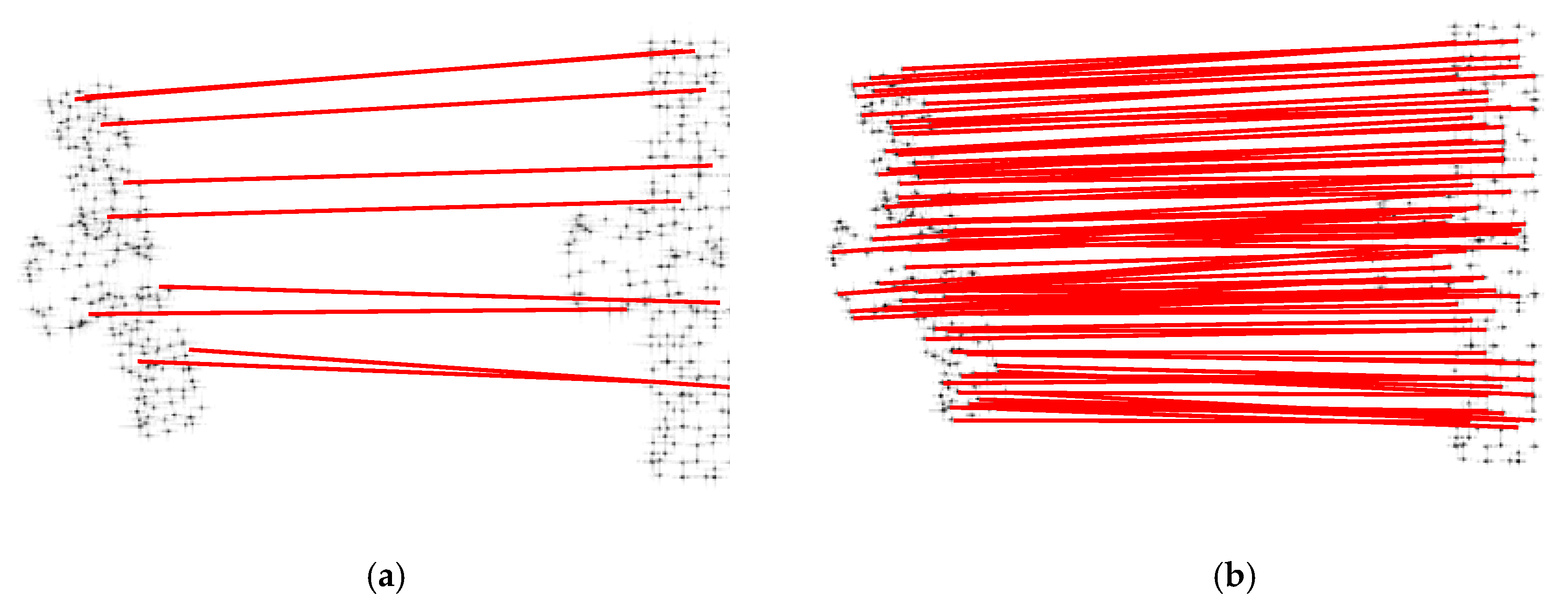
Figure 5 shows the fusion images. Different from modified SIFT, the fusion image from the proposed method is a scatterer image. The line in Figure 5b shows the matched scatterer pairs. One can see that almost all the dominant scatterers are matched in Figure 5b. Because $U$ can represent the relationship between two images, the estimated RMSE of $U$ is used to measure the performance of the algorithm. The RMSE is computed according to

$$\mathrm{RMSE}=\sqrt{\frac{1}{N}{\displaystyle \sum _{i=1}^N{\left(U_i-U_0\right)}^2}}$$

(52)

where $U_i$ is the estimated $U_0$, and $U_0$ is the real value. Using different signal-to-noise ratio (SNR) $(-10,-5,0,5)\mathrm{dB}$, 200 Monte Carlo experiments were carried out. The RMSE of the estimated $U$ is shown in Figure 6a. The performance of the modified SIFT was better as the SNR improved. The proposed method was not affected by the noise in this range. This is because the dominant scatterer extraction algorithm is highly precise. A precise dominant scatterer extraction is the foundation of the proposed method. After feature points matching, the target 3D image can be obtained, as shown in Figure 6b. A comparison of estimated target attitude and the setting target attitude to radar A is shown in Figure 7.

4.2. Simulation based on CADFEKO Software

To verify that the proposed method is suitable for the radar echo close to the real data, an experiment based on CADFEKO software was carried out. The target was a simulated satellite, as shown in Figure 8a. The length and width of the solar panel were 1 m and 0.28 m, respectively. In the middle, there was a sphere, and the diameter was 0.4 m. The distance between the two solar panels was 0.6 m. The setting parameters are listed in

Table 2. Parameter settings.

Parameters	Setting Value
$\phi$	19.69°
ARX	80.00°
ARY	91.73°
Radar A ${\varphi }_A$	20.00°
Radar B ${\varphi }_B$	0.00°

. According to the setting parameters, one can see that the ARX was 80°. However, ARY cannot be directly obtained from the system parameters, which need to be calculated. The unit vectors of radar A and radar B can be expressed as

$${\overrightarrow{n}}_A=\left[\sin \alpha \cos \varphi ,\sin \alpha \sin \varphi ,\cos \alpha \right]$$

(53)

$${\overrightarrow{n}}_B=\left[\sin \alpha \cos \left(\varphi +\psi \right),\sin \alpha \sin \left(\varphi +\psi \right),\cos \alpha \right]$$

(54)

where $\psi$ is the azimuth angle between radar A and radar B; $\varphi$ is the azimuth angle of radar A. Because the $O_0{X}_0{Y}_0$ plane is made of ${\overrightarrow{n}}_A$ and ${\overrightarrow{n}}_B$, the $Z_0$-axis can be expressed as

$${\overrightarrow{n}}_{Z_0}=\frac{{\overrightarrow{n}}_A\times {\overrightarrow{n}}_B}{\Vert {\overrightarrow{n}}_A\times {\overrightarrow{n}}_B\Vert }$$

(55)

Then, the $Y_0$-axis can be expressed as

$${\overrightarrow{n}}_{Y_0}=\frac{{\overrightarrow{n}}_{Z_0}\times {\overrightarrow{n}}_A}{\Vert {\overrightarrow{n}}_{Z_0}\times {\overrightarrow{n}}_A\Vert }$$

(56)

ARY can be represented by

$$\beta =\mathrm{acos}({\overrightarrow{n}}_{Y_0}(3))$$

(57)

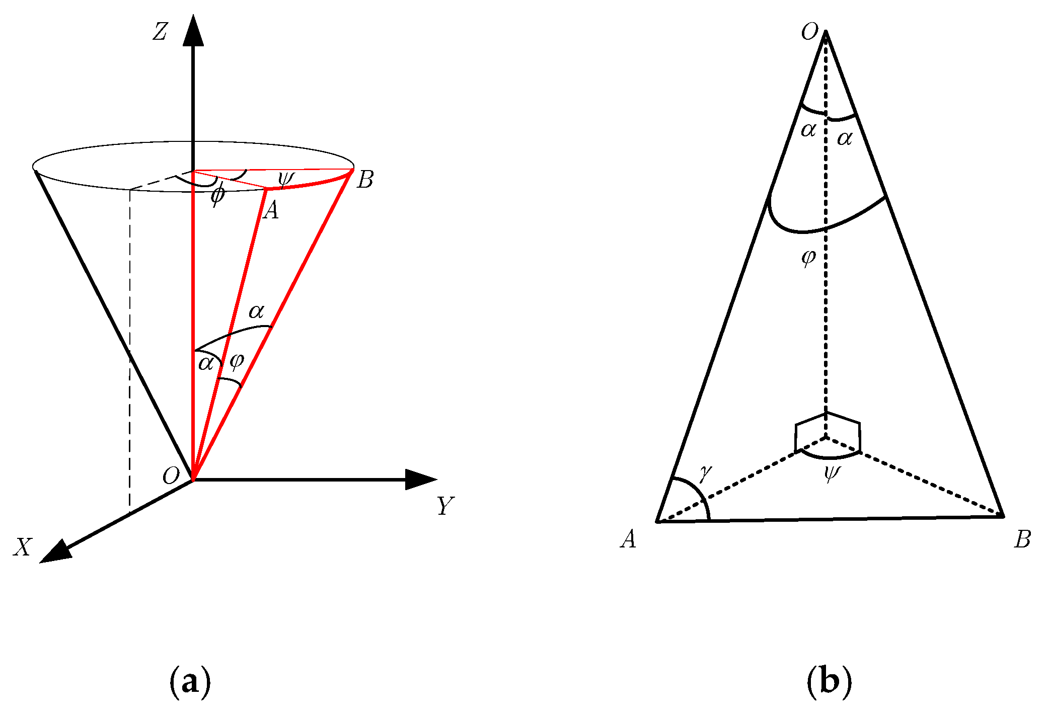
where ${\overrightarrow{n}}_{Y_0}(3)$ is the third element of ${\overrightarrow{n}}_{Y_0}$. $\beta$ is influenced by $\psi$ and $\alpha$, and the relationship is shown in Figure 8b. Because the pitch angle of two radars is the same, $\beta$ is greater than 90° and less than 115°. In addition, $\phi$ cannot be obtained from the preset parameters. The CADFEKO model is abstractly represented in Figure 9a. For the convenience of analysis, the red part of Figure 9a is shown in Figure 9b. $\phi$ can be obtained by

$$\phi =\pi -2\gamma$$

(58)

where $\cos \gamma =\sin \theta \sin (\psi /2)$. As analyzed above, ARY and $\phi$ are calculated as 91.73° and 19.69°, respectively.

.

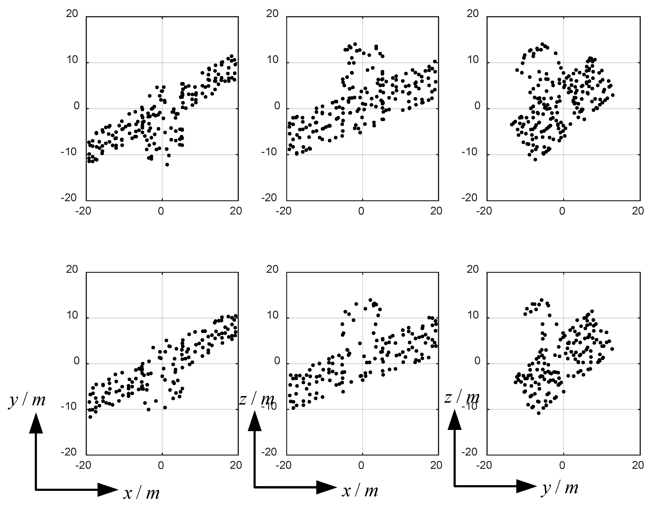
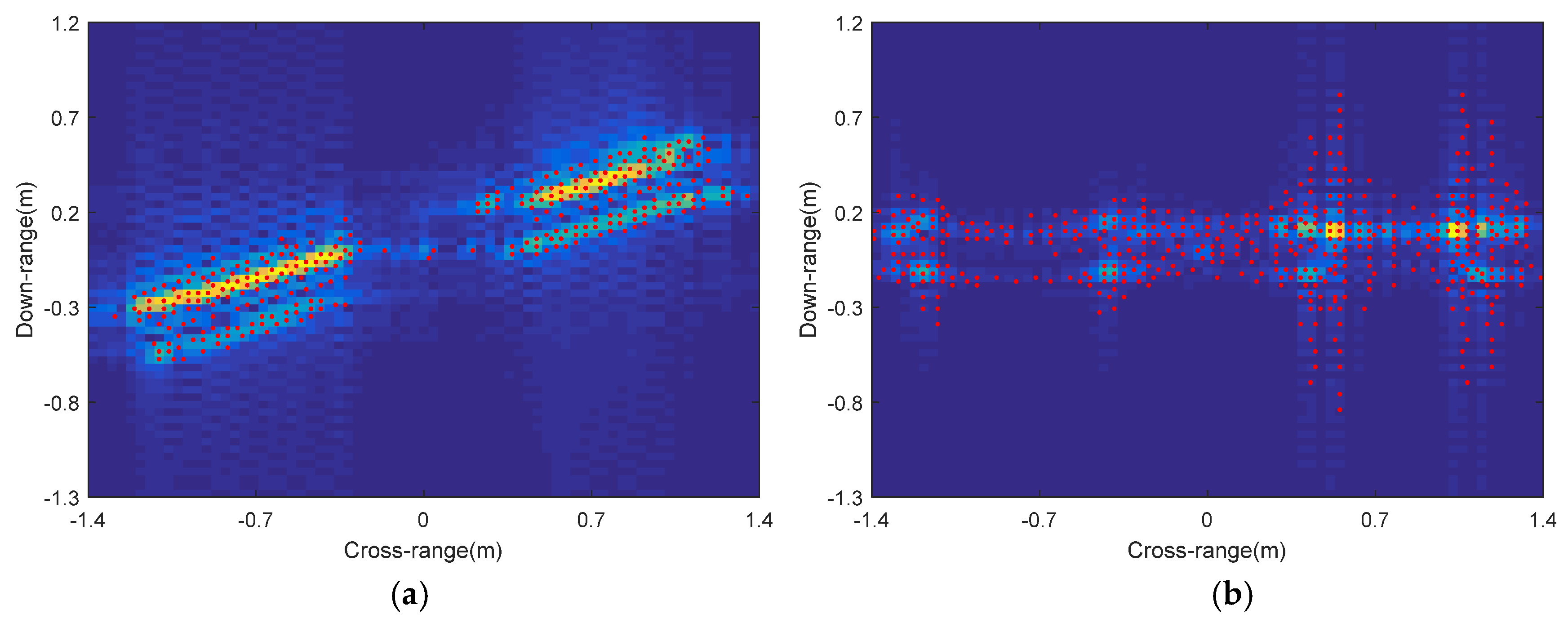
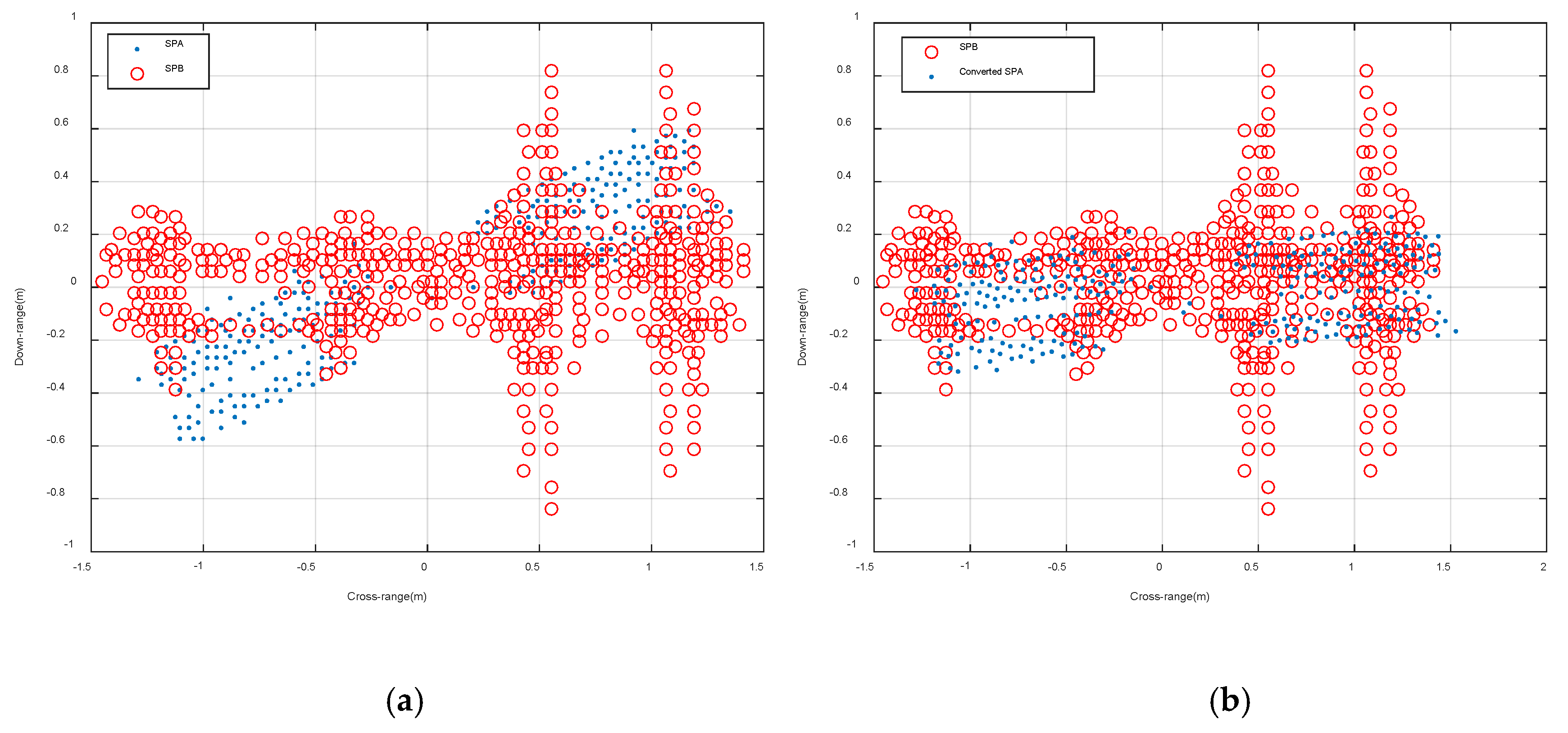
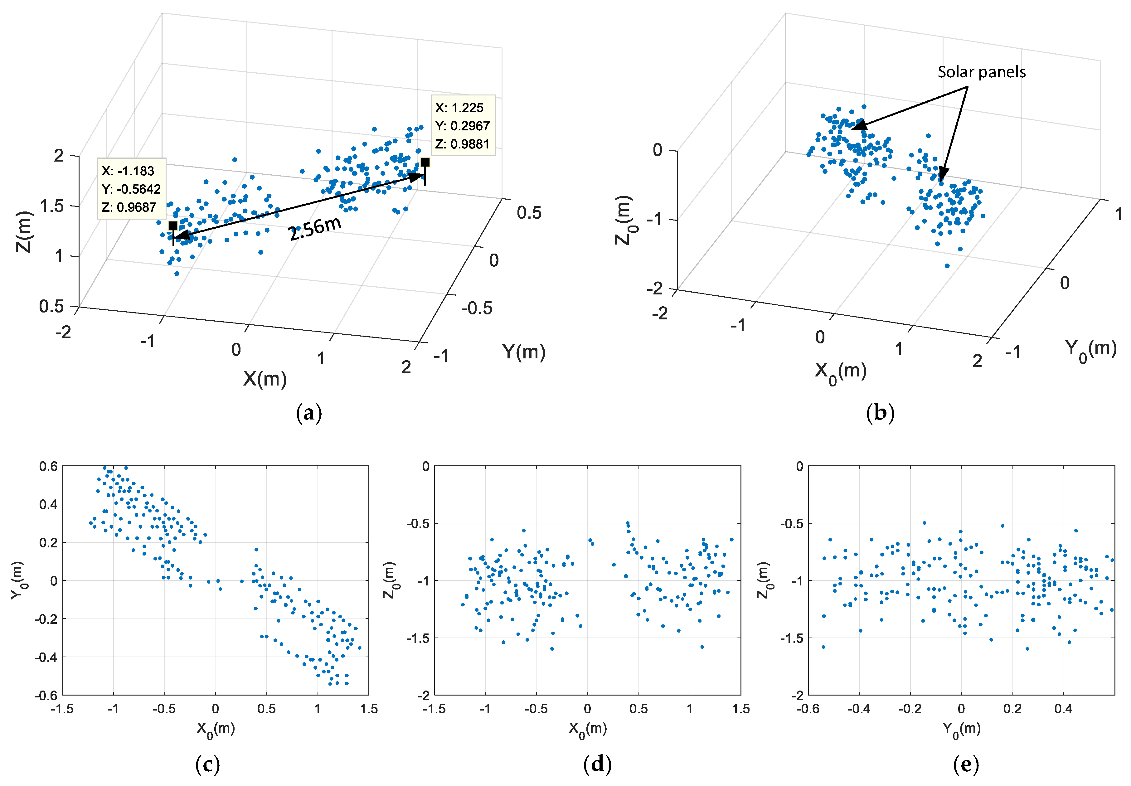
Through scattering center extraction, the extracted SPA and SPB are shown in Figure 10. Figure 10b shows eight edge points with strong sidelobes. Due to the difference in the angle of incidence and the degree of position occlusion at the edge points, its scattering intensity also changed, two of which were significantly larger than the other six. There were also scattering points between the eight edges. After RANSAC, the converted SPA and SPB are plotted in Figure 11b. Since the influence of noise on RANSAC is relatively small, the influence of sidelobes in SPB can be removed after preliminary scattering point matching. After iteration, the target 3D image can be obtained, as shown in Figure 12a. The estimated length of the solar panel was 2.56m. The estimated ARX and ARY are listed in

Table 3. Parameter estimation results.

Parameters	Setting Value	Estimation Error	Estimation Error
ARX	80.00°	75.67°	4.33°
ARY	91.73°	94.38°	2.65°

. According to the estimated ARX and ARY, the 3D reconstruction with respect to the radar coordinate system is shown in Figure 12b, where two solar panels are identified. The three views of Figure 12b are shown in Figure 12c–e. Compared with SPA in Figure 11a, the front view of Figure 12c is bigger and upside down. According to (50) and (51), the top view shows $x$ and $y$ in the radar coordinate system. Figure 11a shows $x_A$ and $y_A$, which is the projection of target to the image plane. This image plane is different from the $(X_0,Y_0)$ plane.

5. Conclusions

In this paper, ISAR image matching and three-dimensional (3D) scattering imaging based on extracted dominant scatterers are studied. Compared with 3D imaging based on an ISAR sequence, the proposed method needs two arbitrary radar observations in a short time. Different from SIFT, the matching process in the proposed method is based on the location of scattering points. Without harsh feature descriptions, the matched scatterers are greatly increased. First, taking advantage of the sparsity of the ISAR image, the radar images are transformed into scattering point sets by scattering the center extraction method. Then, coarse scatterer matching can be achieved by RANSAC. The scatterer height and accurate affine transformation parameters are estimated iteratively to obtain fine scatterer matching. Based on matched scatterers, the target 3D image, ARX, and ARY can be obtained. Finally, experiments based on electromagnetic simulation software CADFEKO have been conducted to demonstrate the effectiveness of the proposed algorithm.

References

- Chen, C.-C.; Andrews, H.C. Target-motion-induced radar imaging. IEEE Trans. Aerosp. Electron. Syst. 1980, 16, 2–14. [Google Scholar] [CrossRef]
- Zhang, Q.; Yeo, T.S.; Du, G. ISAR imaging in strong ground clutter using a new stepped-frequency signal format. IEEE Trans. Geosci. Remote Sens. 2003, 41, 948–952. [Google Scholar] [CrossRef]
- Bao, Z.; Xing, M.D.; Wang, T. Radar Imaging Technique; Publishing House of Electronic Industry: Beijing, China, 2005. [Google Scholar]
- Wang, Q.; Xing, M.; Lu, G.; Bao, Z. Single range matching filtering for space debris radar imaging. IEEE Geosci. Remote Sens. Lett. 2007, 4, 576–580. [Google Scholar] [CrossRef]
- Chen, L.; Liang, B.; Yang, D. Two-Step Accuracy Improvement of Motion Compensation for Airborne SAR with Ultrahigh Resolution and Wide Swath. IEEE Trans. Geosci. Remote Sens. 2019, 57, 7148–7160. [Google Scholar] [CrossRef]
- Wang, D.-W.; Ma, X.-Y.; Chen, A.-L.; Su, Y. High-resolution imaging using a wideband MIMO radar system with two distributed arrays. IEEE Trans. Image Process. 2010, 19, 1280–1289. [Google Scholar] [CrossRef]
- Carlo, N.; Gianfranco, F.; Marco, M. A novel approach for motion compensation in ISAR system. In Proceedings of the EUSAR 2014, 10th European Conference on Synthetic Aperture Radar, Berlin, Germany, 3–5 June 2014; pp. 1–4. [Google Scholar]
- Baselice, F.; Caivano, R.; Cammarota, A.; Pascazio, V.; Ferraioli, G. SAR despeckling based on enhanced winner filter. In Proceedings of the IEEE International Geoscience and Remote Sensing Symposium (IGARSS), Beijing, China, 10–15 July 2016; pp. 1042–1045. [Google Scholar]
- Xu, G.; Yang, L.; Bi, G.; Xing, M. Enhanced ISAR imaging and motion estimation with parametric and dynamic sparse Bayesian learning. IEEE Trans. Comput. Imaging 2017, 3, 940–952. [Google Scholar] [CrossRef]
- Fu, J.; Xu, D.; Xing, M. A novel ionospheric TEC estimation method based on L-Band ISAR signal processing. In Proceedings of the IGARSS 2019, IEEE International Geoscience and Remote Sensing Symposium, Yokohama, Japan, 28 July–2 August 2019; pp. 314–317. [Google Scholar]
- Ferraioli, G.; Pascazio, V.; Schirinzi, G. Ratio-Based NonLocal Anisotropic Despeckling Approach for SAR Images. IEEE Trans. Geosci. Remote Sens. 2019, 57, 7785–7798. [Google Scholar] [CrossRef]
- Wang, J.; Liang, X.; Chen, L.; Wang, L.; Li, K. First Demonstration of joint wireless communication and high-resolution SAR imaging using airborne MIMO radar system. IEEE Trans. Geosci. Remote Sens. 2019, 57, 6619–6632. [Google Scholar] [CrossRef]
- Sheng, J.; Xing, M.; Zheng, L.; Mehmood, M.Q.; Yang, L. ISAR cross-range scaling by using sharpness maximization. IEEE Trans. Geosci. Remote Sens. Lett. 2015, 12, 165–169. [Google Scholar] [CrossRef]
- Gao, Y.; Xing, M.; Zhang, Z.; Guo, L. ISAR imaging and cross-range scaling for maneuvering targets by using the NCS-NLS algorithm. IEEE Sens. J. 2019, 19, 4889–4897. [Google Scholar] [CrossRef]
- Knaell, K.; Cardillo, G. Radar tomography for the generation of three-dimensional images. Proc. Radar Sonar Navig. 1995, 142, 54–60. [Google Scholar] [CrossRef] [Green Version]
- Mayhan, J.; Burrows, M.; Cuomo, K.; Piou, J. High resolution 3D snapshot ISAR imaging and feature extraction. IEEE Trans. Aerosp. Electron. Syst. 2001, 37, 630–642. [Google Scholar] [CrossRef]
- Morita, T.; Kanade, T. A sequential factorization method for recovering shape and motion from image streams. IEEE Trans. Pattern Anal. Mach. Intell. 1997, 19, 858–867. [Google Scholar] [CrossRef]
- McFadden, F.E. Three-dimensional reconstruction from ISAR sequences. Proc. SPIE 2002, 4744, 58–67. [Google Scholar]
- Liu, L.; Zhou, F.; Bai, X.; Tao, M. Joint cross-range scaling and 3D Geometry reconstruction of ISAR targets based on factorization method. IEEE Trans. Image Process. 2016, 25, 1740–1750. [Google Scholar] [CrossRef] [PubMed]
- Wang, F.; Xu, F.; Jin, Y. 3-D information of a space target retrieved from a sequence of high-resolution 2-D ISAR images. In Proceedings of the IEEE International Geoscience and Remote Sensing Symposium (IGARSS), Beijing, China, 10–15 July 2016; pp. 5000–5002. [Google Scholar]
- Wang, F.; Xu, F.; Jin, Y. Three-dimensional reconstruction from a multiview sequence of sparse ISAR imaging of a space target. IEEE Trans. Geosci. Remote Sens. 2018, 56, 611–620. [Google Scholar] [CrossRef]
- Dan, X.; Xing, M.; Xia, X.-G.; Sun, G.-C.; Fu, J.; Su, T. A multi-Perspective 3D reconstruction method with single perspective instantaneous target attitude estimation. Remote Sens. 2019, 11, 1277. [Google Scholar]
- Gianfranco, F.; Francesco, S.; Francesco, S. Three-Dimensional focusing with multipass SAR data. IEEE Trans. Geosci. Remote Sens. 2003, 41, 507–517. [Google Scholar]
- Gianfranco, F.; Antonio, P.; Diego, R. A null-space method for the phase unwrapping of multitemporal SAR interferometric stacks. IEEE Trans. Geosci. Remote Sens. 2011, 49, 2323–2334. [Google Scholar]
- Marco, M.; Daniele, S.; Federica, S.; Nicola, B. 3D interferometric ISAR imaging of noncooperative targets. IEEE Trans. Aerosp. Electron. Syst. 2014, 50, 3102–3114. [Google Scholar]
- Chen, Q.; Xu, G.; Zhang, L.; Xing, M.; Bao, Z. Three-dimensional interferometric inverse synthetic aperture radar imaging with limited pulses by exploiting joint sparsity. IET Radar Sonar Navig. 2015, 9, 692–701. [Google Scholar] [CrossRef]
- Rong, J.; Wang, Y.; Han, T. Interferometric ISAR imaging of maneuvering targets with arbitrary Three-Antenna configuration. IEEE Trans. Geosci. Remote Sensi. 2020, 58, 1102–1119. [Google Scholar] [CrossRef]
- Zhou, J.; Shi, Z.; Fu, Q. Three-dimensional scattering center extraction based on wide aperture data at a single elevation. IEEE Trans. Geosci. Remote Sens. 2015, 53, 1638–1655. [Google Scholar] [CrossRef]
- Wang, G.; Xia, X.-G.; Chen, V. Three-dimensional ISAR imaging of maneuvering targets using three receivers. IEEE Trans. Image Process. 2001, 10, 436–447. [Google Scholar] [CrossRef] [PubMed]
- Xu, X.; Narayanan, R.M. Three-dimensional interferometric ISAR imaging for target scattering diagnosis and modeling. IEEE Trans. Image Process. 2001, 10, 1094–1102. [Google Scholar] [PubMed]
- Ma, C.; Yeo, T.S.; Zhang, Q.; Tan, H.; Wang, J. Three-dimensional ISAR imaging based on antenna array IEEE Trans. Geosci. Remote Sens. 2008, 46, 504–515. [Google Scholar] [CrossRef]
- Ma, C.; Yeo, T.S.; Tan, C.; Tan, H. Sparse array 3-D ISAR imaging based on maximum likelihood estimation and clean technique. IEEE Trans. Image Process. 2010, 19, 2127–2142. [Google Scholar]
- Xu, G.; Xing, M.; Xia, X.-G.; Zhang, L.; Chen, Q.; Bao, Z. 3D Geometry and motion estimations of maneuvering targets for interferometric ISAR with sparse aperture. IEEE Trans. Image Process. 2016, 25, 2005–2020. [Google Scholar] [CrossRef]
- Tomasi, C.; Kanade, T. Shape and motion from image streams under orthography: A factorization method. Int. J. Comput. Vis. 1992, 9, 137–154. [Google Scholar] [CrossRef]
- Aghababaee, H.; Ferraioli, G.; Schirinzi, G.; Pascazio, V. Regularization of SAR Tomography for 3-D Height Reconstruction in Urban Areas. IEEE J. Sel. Top. Appl. Earth Observ. Remote Sens. 2019, 12, 648–659. [Google Scholar] [CrossRef]
- Ma, W.; Wen, Z.; Wu, Y.; Jiao, L.; Gong, M.; Zheng, Y. Remote sensing image registration with modified SIFT and enhanced feature matching. IEEE Geosci. Remote Sens. Lett. 2017, 14, 3–7. [Google Scholar] [CrossRef]
- Duan, J.; Zhang, L.; Xing, M. Polarimetric target decomposition based on attributed scarrering center model for synthetic aperture radar targets. IEEE Geosci. Remote Sens. Lett. 2014, 11, 2095–2099. [Google Scholar] [CrossRef]
Figure 1.
(a) The radar system. (b) Space vector -axis concerning the system.
Figure 2.
Diagrams of the proposed ISAR scatterer matching and 3D imaging algorithm.
Figure 3.
Feature points (a,b) extracted from image A and image B with respect to modified scale invariant feature transform (SIFT). (c,d) extracted from image A and image B with respect to ISAR.
Figure 4.
Feature points matching. (a) Modified SIFT. (b) The proposed method.
Figure 5.
Feature points fusion. (a) Fusion image of the board by the modified SIFT. (b) The proposed method.
Figure 6.
(a) The RMSE of the estimated . (b) The 3D imaging result by the proposed method.
Figure 7.
The target attitude with respect to radar A. (a) The setting target attitude. (b) The estimated target attitude.
Figure 8.
(a) Satellite target in the CADFEKO model. (b) ARY changes according to different ARX and .
Figure 9.
The abstract representation. (a) The abstract CADFEKO model. (b) The red part of (a).
Figure 10.
The result of two-dimensional (2D) imaging and scattering center extraction. (a) SPA; (b) SPB.
Figure 11.
SPA, SPB, and the coarse matching results. (a) SPA and SPB plotted in one image. (b) The result of converted SPA and SPB.
Figure 12.
3D reconstruction results and the three views. (a) 3D imaging with respect to the target coordinate system; (b) the attitude result with respect to radar A; (c) X-Y view of (b); (d) X-Z view of (b); (e) Y-Z view of (b).