Article

Spatiotemporal Dynamics and Environmental Controlling Factors of the Lake Tana Water Hyacinth in Ethiopia

1
Blackland Research Center, Texas A & M AgriLife Research, Temple, TX 76502, USA
2
Spatial Sciences Laboratory, Texas A & M University, College Station, TX 77843, USA
3
Faculty of Civil and Water Resource Engineering, Bahir Dar Institute of Technology, Bahir Dar University, Bahir Dar P.O. Box 26, Ethiopia
4
Department of Civil & Environmental Engineering, Seoul National University, Gwanak-ro 1, Gwanak-gu, Seoul 151-742, Korea
5
Department of Earth and Environment, Florida International University, Miami, FL 33199, USA
6
Program in Public Health, University of California Irvine, Irvine, CA 92602, USA
*
Author to whom correspondence should be addressed.
Remote Sens. 2020, 12(17), 2706; https://0-doi-org.brum.beds.ac.uk/10.3390/rs12172706
Submission received: 9 July 2020 / Revised: 14 August 2020 / Accepted: 17 August 2020 / Published: 21 August 2020
(This article belongs to the Special Issue Remote Sensing of the Aquatic Environments)

Abstract

:
The largest freshwater lake in Ethiopia, Lake Tana, has faced ecological disaster due to water hyacinth (Eichhornia crassipes) infestation. The water hyacinth is a threat not only to the ecology but also to the socioeconomic development of the region and cultural value of the lake, which is registered as a UNESCO reserve. This study aims to map the spatiotemporal dynamics of the water hyacinth using high-resolution PlanetScope satellite images and assesses the major environmental variables that relate to the weed spatial coverage dynamics for the period August 2017 to July 2018. The plausible environmental factors studied affecting the weed dynamics include lake level, water and air temperature, and turbidity. Water temperature and turbidity were estimated from the moderate resolution imaging spectroradiometer (MODIS) satellite image and the water level was estimated using Jason-1 altimetry data while the air temperature was obtained from the nearby meteorological station at Bahir Dar station. The results indicated that water hyacinth coverage was increasing at a rate of 14 ha/day from August to November of 2017. On the other hand, the coverage reduced at a rate of 6 ha/day from December 2017 to June 2018. However, the length of shoreline infestation increased significantly from 4.3 km in August 2017 to 23.4 km in April 2018. Lake level and night-time water temperatures were strongly correlated with water hyacinth spatial coverage (p < 0.05). A drop in the lake water level resulted in a considerable reduction of the infested area, which is also related to decreasing nutrient levels in the water. The water hyacinth expansion dynamics could be altered by treating the nutrient-rich runoff with best management practices along the wetland and in the lake watershed landscape.

Graphical Abstract

1. Introduction

Aquatic invasive species threaten ecological and socioeconomic integrity by affecting the productivity and functionality of freshwater systems. Water hyacinth (Eichhornia crassipes) is one of the dangerous invasive aquatic weeds, which is native to the Amazon Basin [1,2,3]. When a conducive environment exists, water hyacinth can produce an annual biomass of 50–60 t/ha and doubles its area coverage every 6–15 days [2,4]. Its high tolerance to different environmental conditions such as pH and nutrient level [5,6] combined with its rapid growth and formation of dense impenetrable mats make it a unique weed with a severe potential negative effect to freshwater ecosystems. Water hyacinth exists as a major weed in more than 50 countries such as Zimbabwe, South Africa, and Ethiopia [7,8,9], where it is prevalent in tropical and subtropical regions [10]. In Ethiopia, it was observed the first time in 1974 in the Koka hydropower reservoir [11]. In Lake Tana, the water hyacinth was observed in 2011 [12,13]. The alarming expansion of the weed in Lake Tana since 2017 has attracted wider scientific and public attention.
Lake Tana has a significant ecological, religious, historic, and economic importance. The lake is home to more than 37 islands with historical churches and more than 20,000 inhabitants [14]. Due to the lake’s rich biodiversity and cultural and historical significance, it is registered as the United Nations Educational, Scientific, and Cultural Organization’s (UNESCO) biosphere reserve in 2014. This helps to facilitate the protection of the lake biodiversity, conduct research, and attract more visitors. However, a recent rapid expansion of water hyacinth has posed a major threat to the lake’s biodiversity and socioeconomics activities. The weed has severely disrupted ecological and socioeconomic functions such as aquatic food chain, nutrient cycling, agricultural activities, tourism, transportation, cultural and religious practices, and public health issues [15,16]. The weed’s impact is, in fact, substantial in Lake Tana where the ecological, socioeconomic, and cultural activities are highly intertwined. Understanding the spatial and temporal dynamics of water hyacinth, and factors affecting the spatial dynamics are critical in implementing mitigation measures to limit the expansion, and eventual elimination before the lake’s biodiversity and socioeconomics become in jeopardy.
Managing and controlling the extent of water hyacinth in Lake Tana is paramount to save its unique biodiversity. The management should include effective and frequent monitoring of the water hyacinth expansion both spatially and temporally. The monitoring of water hyacinth can be conducted using conventional methods and remote sensing approaches. Conventional approaches monitor the water hyacinth situation on the ground using tracking devices such as a global positioning system (GPS). The conventional approach requires extensive manpower, funding, and infrastructural setup, which are difficult to sustain in developing countries. On the other hand, freely available remote sensing data and GIS applications can make monitoring of water hyacinth and other aquatic weeds convenient and less costly [17,18].
In the recent past, various studies have addressed the water hyacinth infestation [12,19,20,21,22,23]. The preliminary survey of water hyacinth infestation by Tewabe [12] between October and November of 2011 indicated the earliest infestation of the water hyacinth at the mouth of the Megech River. The effect of water hyacinth infestation on fishing in Lake Tana was evaluated by Asmare [19], which reported the impact of the weed on the fishing industry. The study indicated how the entangling of fishing nets and boat propeller had made the fishing task exhaustive and affected the livelihood quality of the fishermen [19]. Dersseh, et al. [20] mapped water hyacinth infestation hotspot using a GIS-based multi-criteria evaluation technique and estimated the water hyacinth infestation susceptible area. Dersseh, et al. [21] used a Sentinel-2 satellite image to determine the spatial coverage of water hyacinth in the lake. This study builds on previous studies using finer resolution satellite images from PlanetScope to map the spatial distribution of water hyacinth as well as to evaluate major environmental factors affecting the water hyacinth infestation in Lake Tana. The specific objectives of this study are to (1) determine the spatial and temporal distribution of water hyacinth in Lake Tana and (2) identify the major environmental factors that are related to the water hyacinth temporal and spatial dynamics. The findings of this study will provide timely knowledge that is helpful to reduce the water hyacinth infestation in the lake and thereby improving the health of Lake Tana to ensure sustainable ecosystem services.

2. Materials and Methods
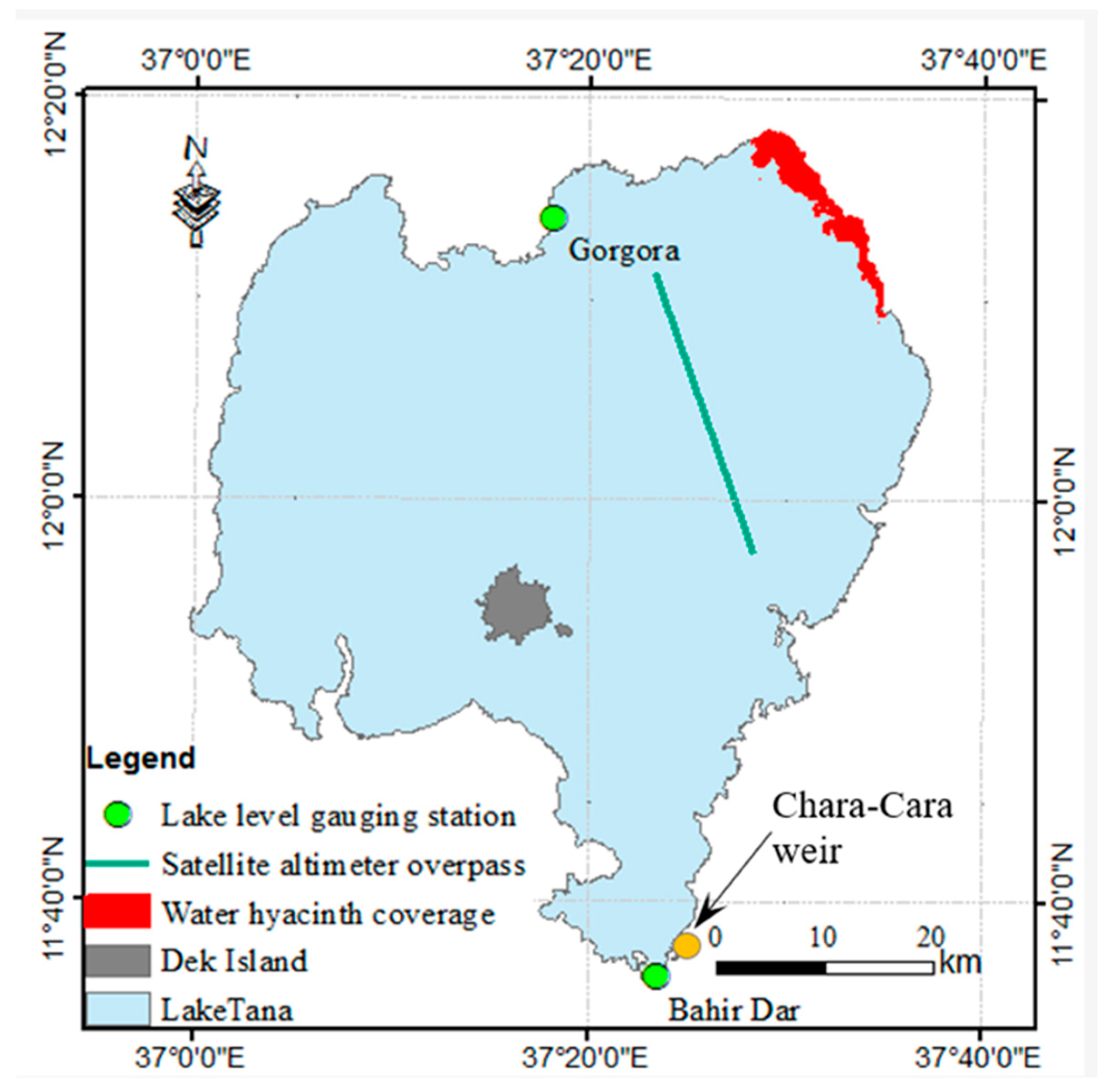
2.1. Study Area

Lake Tana is the largest freshwater lake in Ethiopia, and it is the source of the Upper Blue Nile River. The Upper Blue Nile River contributes more than 50% of annual streamflow to the Nile River [24,25]. Lake Tana has a catchment area of 15,000 km2, out of which the lake covers 20%. The lake is located in the north-west highland of Ethiopia; its exact geographic coordinate extends between 10°45′54.1′′ N, 36°10′24.9′′ E and 12°50′15.9′′ N, 38°50′54.48′′ E (Figure 1).
The lake provides substantial socioeconomic services. For example, more than 2 million people live in the Lake Tana catchment depending for their livelihood directly or indirectly on the lake and its resources [26,27]. The Lake Tana catchment, due to its potential suitable land and climate, it is considered as one of the agricultural growth corridors by the government of Ethiopia [28].

2.2. Lake Tana Hydrology
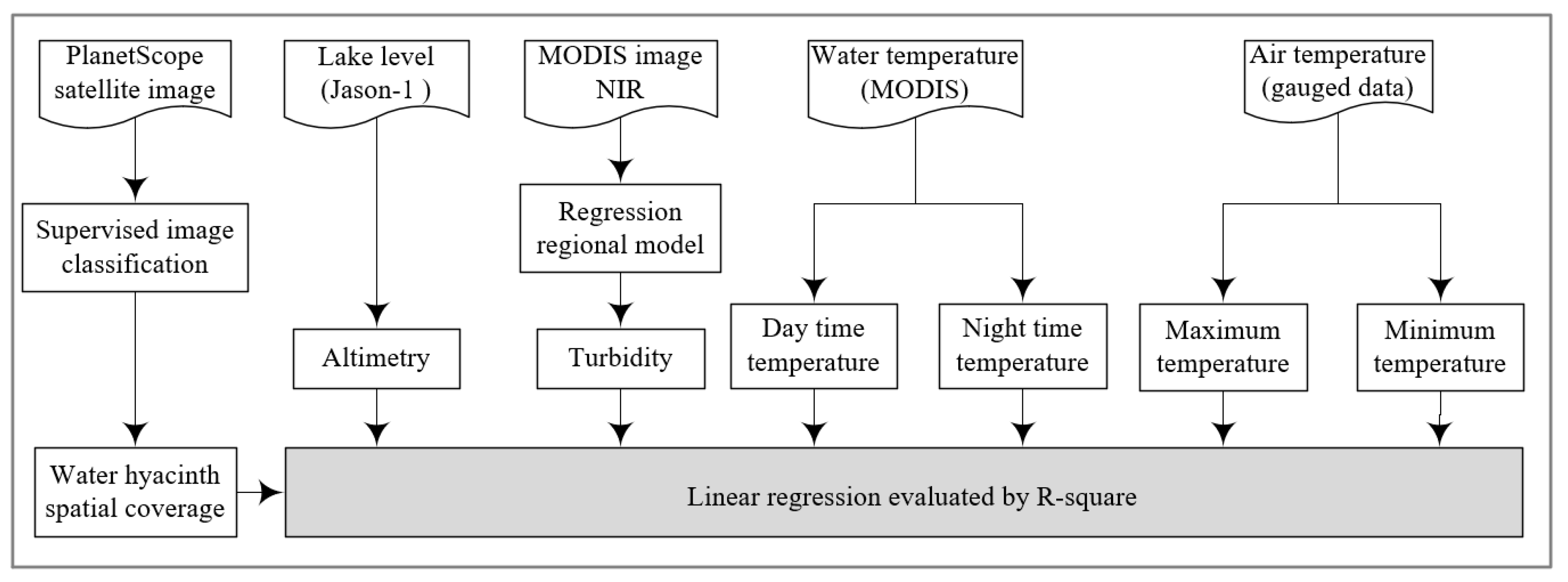
In general, the lake has two main seasons. The main rainfall season is called “Kremt” and it extends from June to September and accounts for 90% of the annual rainfall (Figure 2). The dry season extends from October to May and it is characterized by high daily temperature. According to data from the Bahir Dar meteorological station, the annual average rainfall (1994–2016) in the area is 1490 mm. The average minimum and maximum temperature at Bahir Dar meteorological station (1994–2016) were 9 and 25 °C, respectively (Figure 2). In the Lake Tana watershed, four major rivers contribute about 93% of the streamflow into the lake [29]. Among the largest tributary river, Gilgel Abay contributes 50% of the streamflow followed by Gumara 32%, Ribb 12%, and Megech 6%. These rivers carry a substantial amount of sediment, nutrient, and other pollutants into the lake [30,31,32]. The lake annual evaporation is reported in the range of 1500–1690 mm [29,33], which is greater than the annual rainfall. The lake is considered as shallow with a mean and maximum depth of 12 and 17 m, respectively [30,34].

2.3. Methods

The spatial and temporal distribution of the water hyacinth was mapped from August 2017 to July 2018 using high-resolution satellite images from the PlanetScope (https://www.planet.com/). Details of the satellite image processing are presented in the following section. The potential environmental factors that affect the water hyacinth spatial dynamics studied were lake water level, air and water body temperature, and lake water turbidity. The water body temperature and lake water turbidity were estimated from the moderate resolution imaging spectroradiometer (MODIS) images. The air temperature was obtained from the Bahir Dar weather station, which is the closest meteorological station to the lake. The observed lake level was assimilated with altimetry lake level data from Jason-1 and Jason-2. The mapped spatial coverage of water hyacinth was compared with the environmental factors to identify the factors that played a role in the spatial dynamics of the water hyacinth coverage. The applied methodology to map water hyacinth coverage, identify major factors plausibly contributing to the weed dynamics, and determine their association is presented in Figure 3.

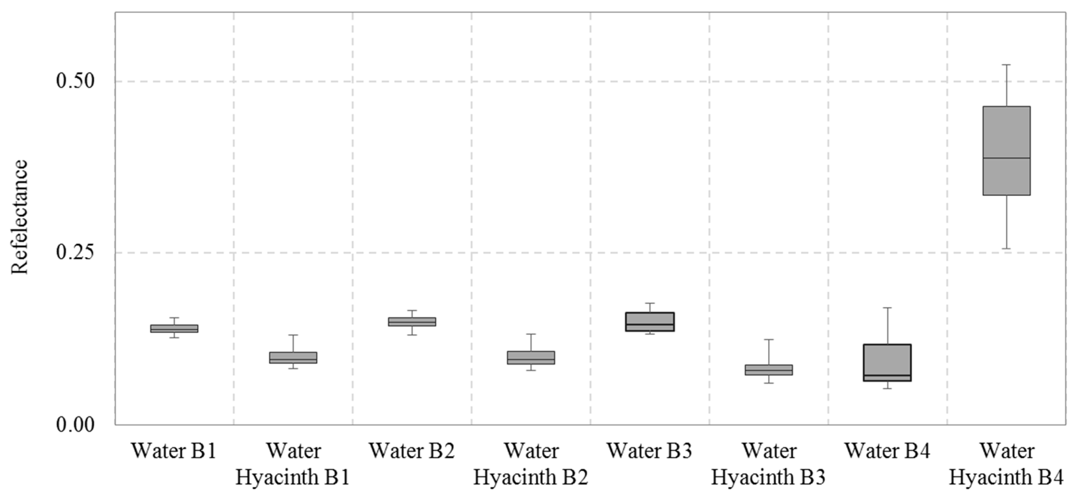
2.3.1. Spatiotemporal Water Hyacinth Distribution Mapping

Effective water hyacinth management requires close monitoring of the spatiotemporal coverage. The conventional way of monitoring using a tracking device requires a sustained funding necessary infrastructure and operational setups. Therefore, it is economically and practically expensive to have effective conventional monitoring for a vast lake such as Lake Tana. Rather, the use of satellite data and GIS applications have become more practical and economically viable to map the spatial distribution of aquatic weeds [35,36]. This study uses a high-resolution satellite image from Planet Constellation to capture the spatial and temporal distribution of the water hyacinth in Lake Tana. Since 2013, Planet Constellation images the entire Earth and the climate every day to make the global change detectable, accessible, and actionable [37,38]. The Planet Constellation operates PlanetScope and RapidEye Earth-imaging constellations [39]. With more than 175 satellites in orbit, it has the largest fleet of Earth observation satellites [40]. Since the PlanetScope has a relatively finer resolution than RapidEye, this study used PlanetScope to map the spatial distribution of the weed coverage. PlanetScope has a daily revisit with a spatial resolution of 3–5 m in the visible (455–515 nm, 500–590 nm, and 590–670 nm) and near-infrared (780–860 nm) spectrum [37].
The PlanetScope satellite image for the Lake Tana area was collected since 9 August 2017. Between August 2017 and July 2018, twelve images free of cloud cover were chosen as presented in the annex (Table S1). Emphasis was given to the northeast shore of the lake, where there is extensive water hyacinth infestation. PlanetScope provides geometrically corrected images using highly accurate distributed ground control points [41,42]. To maintain consistency between sensory and overpass time, the metadata provides assets to evaluate the quality of the pixel and coefficients necessary to convert the radiance to reflectance. In this study, the selected satellite images were preprocessed to convert the raw data to reflectance using the coefficients provided. The preprocessed satellite image was classified with a maximum likelihood supervised classification method [43]. The maximum likelihood classification algorithm is exceptionally suitable for our study in that the inverse matrix of the variance–covariance matrix is very stable due to the very low correlation between the bands used in the classification. The representative training samples distributed across the selected images were collected on individual images. The supervised classification on 25 June 2017 was validated using water hyacinth coverage tracked with a boat and handheld GPS and then after validation a similar supervised classification was applied on the selected images.

2.3.2. Major Factors Affecting Water Hyacinth Spatial Coverage Dynamics

Plant growth is affected by a complex interaction of environmental factors such as climatic conditions and nutrient availability [44,45,46]. Suitable climate and abundant nutrient availability ensure convenient conditions for vegetation growth in the aquatic environment [47,48]. The environmental factors studied to assess their impact on water hyacinth growth in the Lake Tana include air and lake water temperature, lake level, and lake water turbidity.
Lake depth: Morphometric characteristics influence the ecological processes in a lake. The lake depth, for example, affects the thermal stratification, which in turn influences dissolved oxygen levels. Depth also limits the type of weed growing in a portion of the lake. Floating weeds can survive in a deeper section of the lake and avoid nutrient competition with shallow-rooted crops. Water hyacinth thrives both as a free-floating or rooted weed as it adjusts to the depth of the water. The depth of the water hyacinth infested area was characterized based on a recent bathymetry survey conducted by the Tana Sub-basin Organization (TaSBO) in 2011. This survey is better than the surveys conducted by Pietrangeli [49] and Ayana [50] since it has more data points that enabled a robust depth interpolation. The bathymetry survey was interpolated with Inverse Distance Weighting (IDW) and overlayed with the historical water hyacinth infested area to evaluate the lake depth infested with water hyacinth.
Air and lake water temperature: Temperature affects plant development and growth by regulating biochemical processes and photosynthesis activity [51]. Air temperature regulates water body temperature. In fact, its effect is significant over shallow lakes [52]. Plants have a defined range of minimum and maximum temperatures within which growth occurs, and at optimum temperature, the plants grow at a faster rate [53,54]. Kasselmann [55] reported that the minimum (base) and optimum temperatures for water hyacinth growth are 10 °C and 25–30 °C, respectively. The daily air temperature was obtained from the closest weather station to the lake, which is located in Bahir Dar city. The day and night water temperature were obtained for the period 2010–2018 from a moderate resolution imaging spectroradiometer (MODIS) MOD11A2 product. MOD11A2, which is available at 1 km spatial and 8-days temporal resolution. MOD11A2 product has been used for the monitoring of inland water bodies [56,57,58]. Since the water hyacinth infested area is covered by the green vegetation, water body temperature was extracted at a 2 km buffer distance from the water hyacinth infestation. Since short vegetation over water can be expected to alter the water surface temperature relative to the adjacent non infested water surface [59,60,61], the nearby water temperature is assumed to be representative. The monthly average day and night-time water temperature, and minimum and maximum air temperature were compared with the water hyacinth spatial coverage to assess if they impact the spatial dynamics of the water hyacinth.
Lake level: The lake level was measured at two diametrically opposite locations since 1960 at Bahir Dar and Gorgora (Figure 4). However, both of these lake level measuring stations were far from the location where a major water hyacinth infestation was observed. The water level gauged data from these stations may be susceptible to bias due to the backwater curve effect from the Chara-Chara weir, which was built in 1996 to regulate the outflow of the lake through the Blue Nile river. The lake water level data is available until 2006 and it does not cover the study period. These drawbacks compelled us to use remotely sensed lake level data from TOPEX/POSEIDON, Jason-1, and Jason-2. These data are available at 10-day intervals since 1993 [62]. The altimeter tracks over Lake Tana were the closest water level measurement to the study site (Figure 4). The altimetry data were compared with gauged lake level data, which was measured before the construction of the weir (i.e., 1993–1996). The validated altimetry data, which is available at near-real-time was used to evaluate the association of the lake level on weed dynamics during the study period (August 2017 to July 2018).
Turbidity: Turbidity is the most widely used parameter to evaluate physical water quality. It is used to evaluate the cloudiness of given water in comparison to a clear water standard [63]. A lake gets turbid because of the inflow of suspended sediment and dissolved materials through the major tributary rivers. Higher turbidity is considered as an indicator of higher suspended sediment concentration and consequently higher nutrient inflow. Excess availability of nutrients may result in the growth of aquatic crops [64]. Comparing the change in turbidity to the change in spatial coverage of the water hyacinth dynamics may provide insight if the nutrient inflow is the cause for the expansion of the water hyacinth in Lake Tana.
Lake water turbidity data is not available for the Lake Tana. Rather, calibration coefficients from previous studies [31,65,66] were used to estimate Lake Tana’s turbidity from MODIS satellite images. Ayana, et al. [31] showed a strong linear association between in situ measurements of turbidity (NTU) and reflectance of MODIS near-infrared channel (NIR) of the electromagnetic spectrum (620–670 nm). Turbidity estimation using NIR has been widely applied for monitoring the water quality of water bodies in different regions and provides a spatial perspective of the water quality of large water bodies [31,65,66,67,68,69,70].
This study used a 500 m resolution and 8-days revisiting time MODIS satellite NIR images to generate the long-term (2010–2016) average spatial turbidity of the lake. The average monthly historical turbidity for the study period was also estimated in the proximity of the historical water hyacinth infestation area at 2 km buffer distance and used to compare with the weed spatial extent for the study duration (August 2017 to July 2018).

3. Results

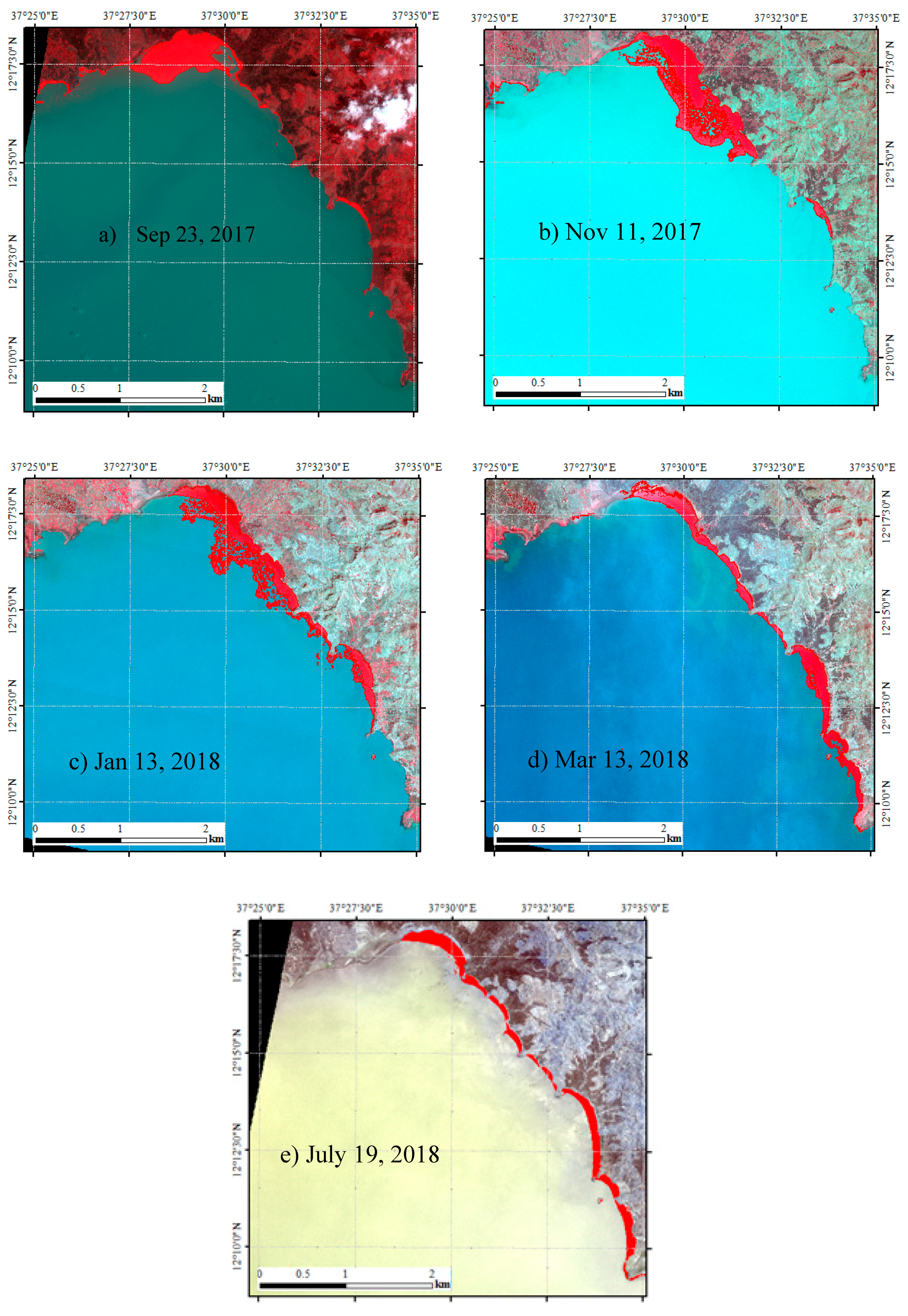
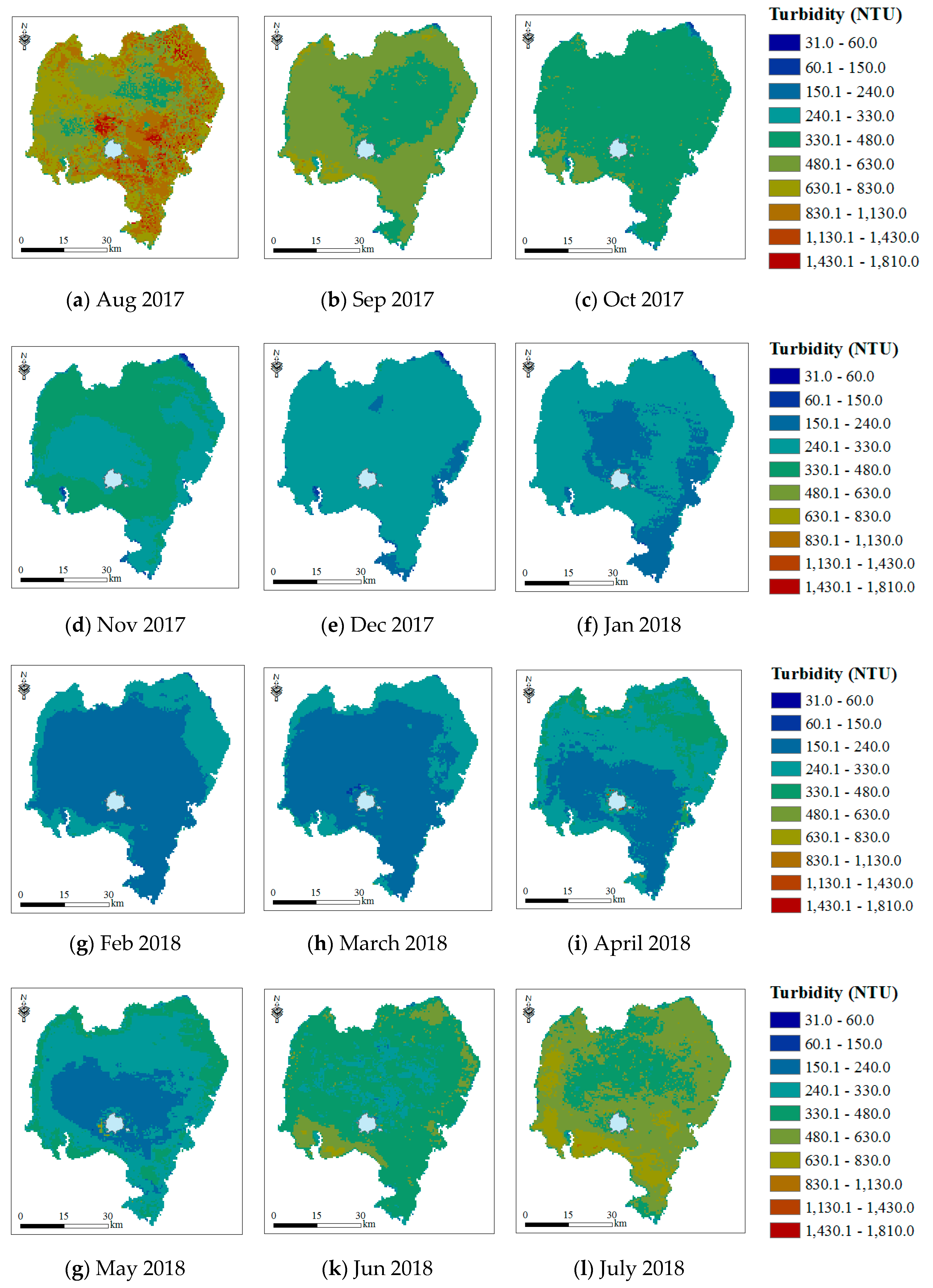
3.1. Water Hyacinth Spatiotemporal Dynamics

The visual inspection of the PlanetScope images showed a large infestation of aquatic weed in the northeast shore of Lake Tana. Figure 5 presents the reflectance of the water hyacinth and waterbody at 56 selected pixels on the satellite images across the study area over the selected satellite images (Table S1). The one-way analysis of variance (ANOVA) on the reflectance of the aquatic weed and waterbody indicated a significant difference in reflectance between band 1, 2, 3, and 4 (p < 0.05). The difference in the near-infrared wavelength (band 4) was very high since water has relatively lower reflectance while water hyacinth (green vegetation) has higher reflectance in this range. Therefore, a supervised classification was implemented by developing an image mosaic of bands 4, 3, and 2 to map the spatial extent of the water hyacinth.
The selected PlanetScope imagery (Table S1) was classified using a supervised classification technique to determine the spatial coverage and length of shoreline infestation (Figure 6). The water hyacinth spatial coverage estimated with a supervised classification on October 25, 2017, was compared with the water hyacinth coverage tracked at the ground with GPS attached on a boat. The comparison of tracked water hyacinth coverage collected with a handheld GPS (June 25, 2017) was compared with the corresponding water hyacinth coverage mapped with supervised classification on October 24, 2017, the result indicated more than 84% match (Supplementary Information (SI), Figure S1). The difference in the agreement was due to the one-day overpass gap between the satellite image and GPS tracking, as well as the fast growth and movability of the water hyacinth.
Figure 7 presents the spatial coverage of the water hyacinth of the selected images during the study period (Table S1). The water hyacinth was first observed in the northern shore of the lake (Figure 7a). A significant proportion of the weed moved to the northeast and expands to the eastern shore of Lake Tana (Figure 7a–e). According to the satellite images, for the period August to November 2017, the water hyacinth was expanding at a rate of 14 ha/day and covered 1600 ha of the lake. On the other hand, the coverage decreased at a rate of 6 ha/day from December 2017 to June 2018. The lowest water hyacinth coverage was observed in June 2018 at 300 ha. Despite the area reduction for the period August 2017 to July 2018, the length of water hyacinth infestation was increasing across the lake shoreline. The maximum infestation length was 23.8 km in April 2018 (Figure 6).

3.2. Environmental Factors Plausibly Contributing to the Water Hyacinth Dynamics

The water hyacinth spatial dynamics in Lake Tana is influenced by environmental and human factors. Identifying the major factor requires a detailed analysis of field data. The environmental factors that could affect the water hyacinth dynamics may include air and lake water temperature, turbidity, lake level, and the human factors (i.e., manual and mechanical harvesting of water hyacinth). In this study, the plausible environmental factors associated with the water hyacinth dynamics were studied.

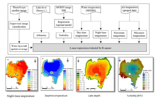
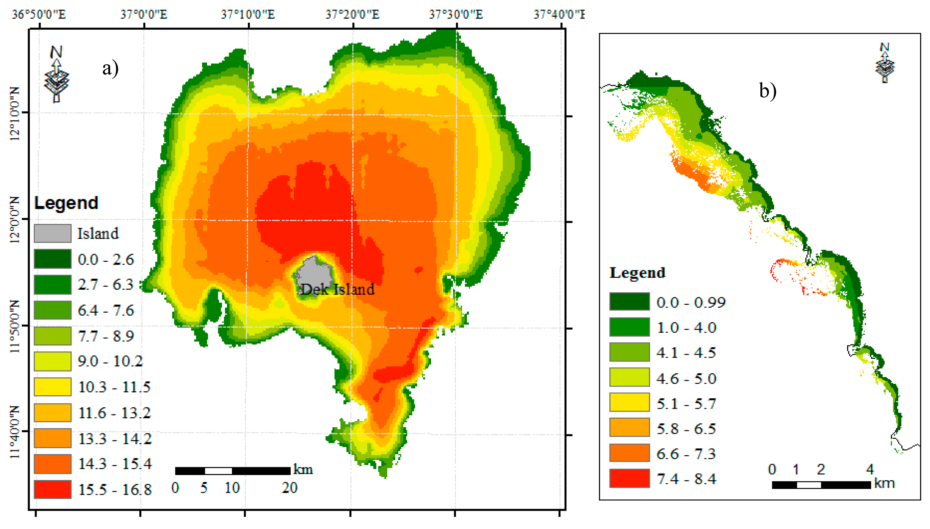
3.2.1. Lake Tana Bathymetric Survey

The bathymetric survey by TaSBO interpolated with IDW revealed a new maximum depth higher than the previously reported depth of 14 m [30,34,71,72]. The bathymetric survey indicated a maximum and average depth of the lake as 16.8 and 12 m, respectively. The depth map (Figure 8) indicated that the lake depth across the historical water hyacinth infestation area for the study period varied between 0 and 8.4 m. Approximately 28% and 37% of the water hyacinth floats on the lake depth less than 0.6 and 1.0 m, respectively (Figure 8b). This suggests that more than half of the water hyacinth could only be harvested with a mechanical harvester since manual harvesting by hand on a water depth greater than one meter could be dangerous. Therefore, integration of manual and mechanical harvesting controls is vital for the removal of water hyacinth in Lake Tana.

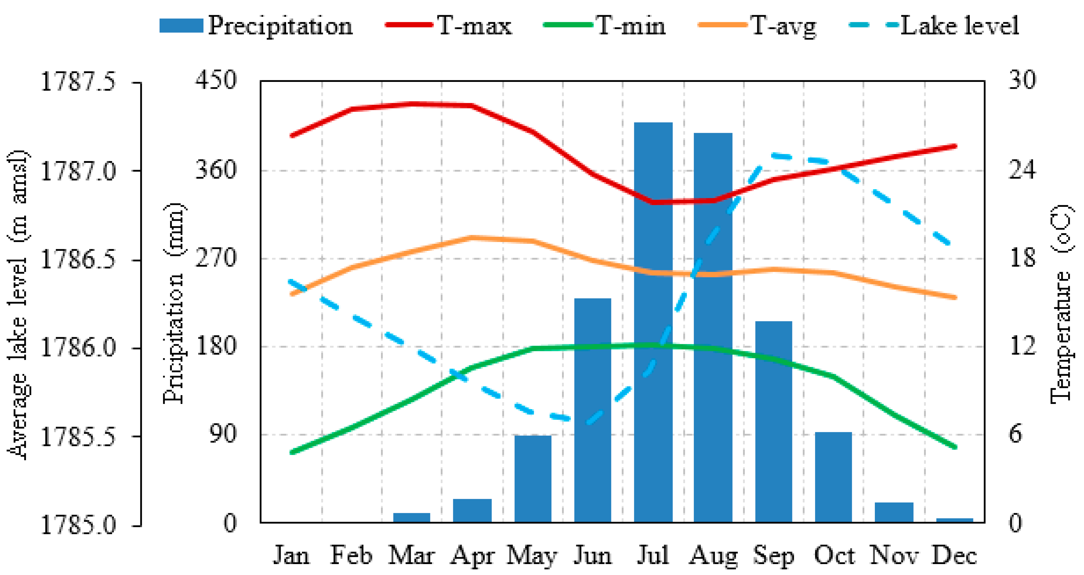
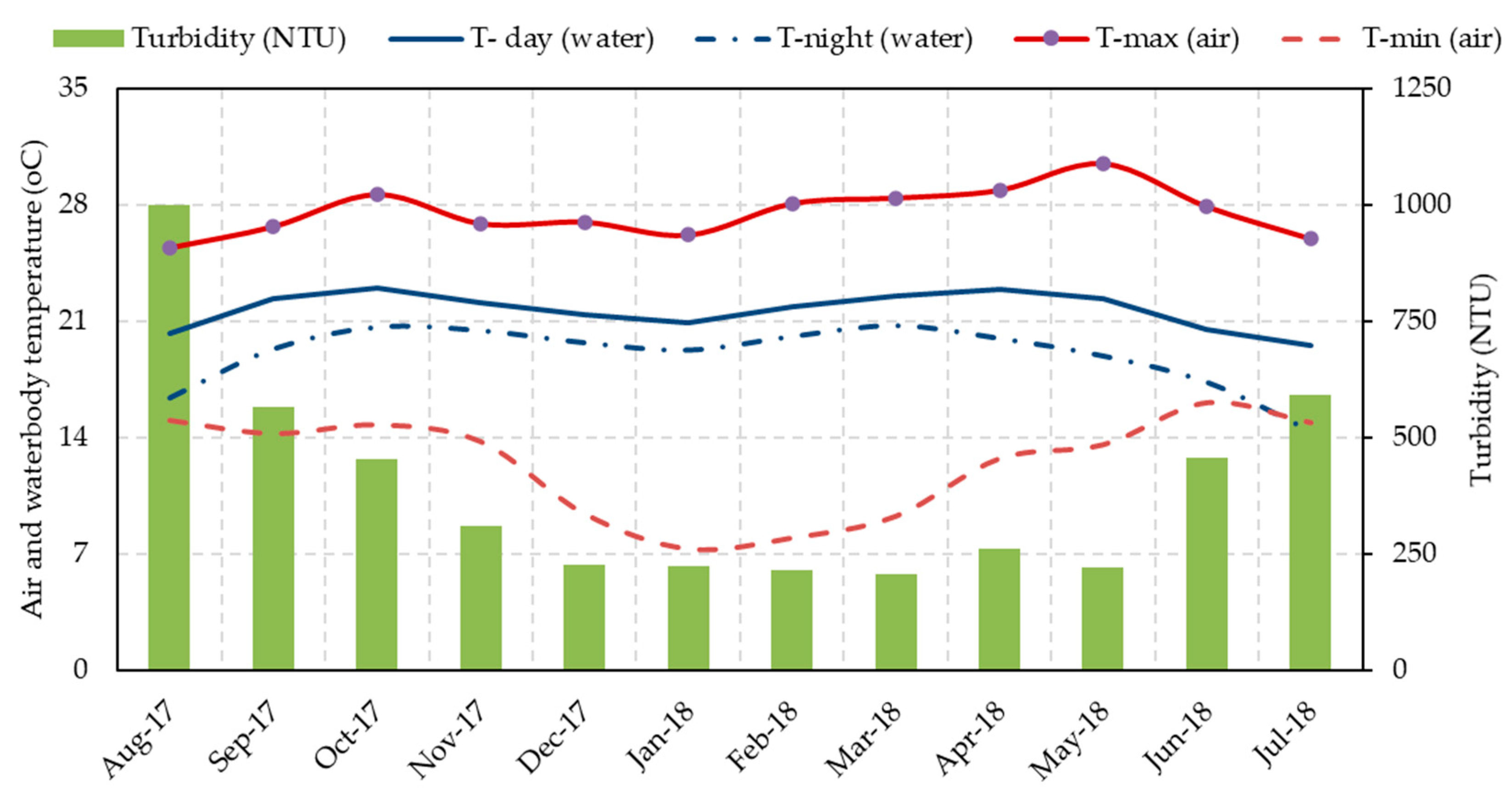
3.2.2. Air and Water Temperature
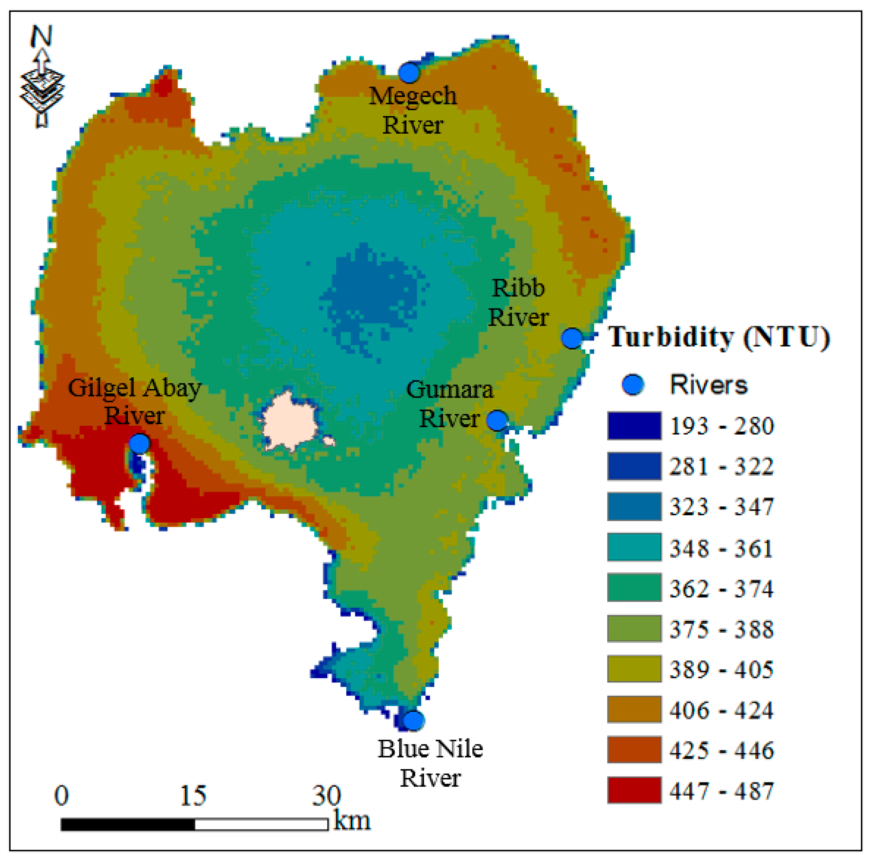
The average annual day and night-time water temperature for Lake Tana were estimated from the MODIS satellite image for the period 2010–2016 (Figure 9a,b). For this period, the annual average daytime water temperature ranged from 20.7 to 33.9 °C, averaging at 22 °C. The northern and central parts of the lake were cooler in the daytime (Figure 9a). The daytime temperature indicated higher spatial variability with a standard deviation of 1.9 °C compared to that of the night-time temperature, which had a standard deviation of 0.6 °C. The night-time temperature was warmer in the northeast shore of the lake where there is water hyacinth infestation (Figure 9b), and ranges between 14 and 19.9 °C, averaging at 18.4 °C. The northeastern side of the lake is also characterized by shallow depth with a gentle slope.
The monthly average day and night-time water temperatures were estimated for the 2 km buffer zone along with the water hyacinth coverage for the period August 2017 to July 2018 (Figure 10). Since water is a slow conductor of heat compared to air, the night and daytime water temperature were within the maximum and minimum air temperature (Figure 10). The water temperature was above the base temperature of the water hyacinth throughout the year; however, the minimum air temperature was below the base temperature of the water hyacinth during the period December to April. Perhaps, the lower minimum air temperature from December to April may contribute to the decrease in water hyacinth coverage although the decrease of the water hyacinth coverage continues until June-July (Figure 6).

3.2.3. Turbidity

Turbidity in Lake Tana is highly variable in both space and time. The average annual turbidity estimated for the period 2010–2016 is presented in Figure 11. The average annual turbidity of the lake was 348 nephelometric turbidity units (NTU) with a standard deviation of 30 NTU. Turbidity less than 25 NTU is relatively considered as clear and at 2000 NTU is completely opaque [73]. The highest turbidity was observed in the southwest shore of the lake near Gilgel Abay river mouth followed by the northeast part of the lake (Figure 11). The higher turbidity is due to sediment carried with the tributary rivers. For example, a Landsat image in December 1984 and December 2017 indicated that the river mouth delta at the entrance of Gilgel Abay to the Lake Tana increased from 12.7 to 21.8 km2 (an increase by 72%; see Supplementary Information, Figure S2). Likewise, the river entrance deltas for Gumara and Ribb rivers were also increasing, but at a lesser extent. Since Gumara and Ribb rivers drop the sediment at the Fogera floodplain, the sediment contribution of both rivers was relatively smaller [74,75]. The floodplains play a critical role by intercepting and trapping nutrient and sediment loadings that are transported with streamflow. Protection of the lake ecosystem should consider implementing best management practices along the watershed landscape and protecting the wetland.
The monthly average turbidity of the lake is shown in Figure 12. The highest turbidity was observed during the major rainfall season (June–September) where the rivers drain to the lake bringing the sedimentation laden water from upland agricultural watersheds. The turbidity of the lake is very low during the dry season (November–May) with average turbidity ranging between 225 and 330 NTU. In the northeast corridor, turbidity becomes high in August after two months from the beginning of the main rainfall season. The monthly average turbidity (August 2017 to July 2018) within the proximity (2 km buffer) of the water hyacinth infestation (Figure 10) was estimated from MODIS images.

3.2.4. Lake Level Variation

Comparison between ground-based and that of Jason-1 altimetry mission water level measurements before the construction of the Chara-Chara weir (i.e., 1993–1996) showed a very strong agreement (R-square of 0.96, p < 0.05, Figure 13) with a root mean square error of 15 cm. Jason-1 altimetry data has also captured well the observed lake level of several lakes of different size [50,76,77]. The altimetry data showed an annual average lake level fluctuation of 1.5 m for the period 1994–2010. This fluctuation was primarily driven by lake rainfall and streamflow during the major rainfall season. The lake level started rising in June, where rainfall started and reached a maximum level in September and declines linearly towards June of the following year (Figure 2). Given the Jason-1 altimetry data represented the lake level, and that it has data for the study period (August 2017 to July 2018), it was used to understand the relationship between lake level and water hyacinth spatial coverage dynamics.

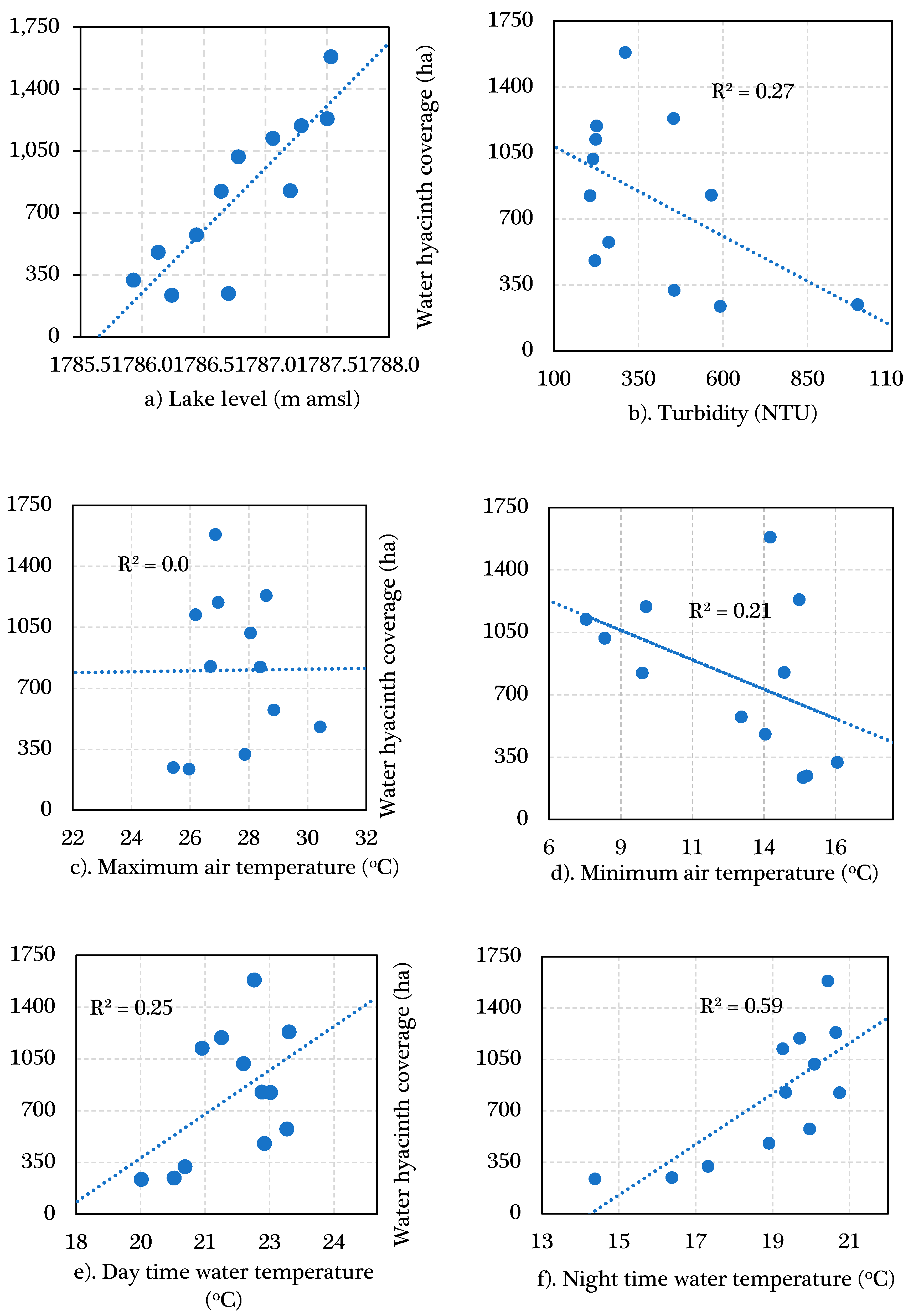
3.3. The Interplay between Environmental Factors and Water Hyacinth Coverage

The environmental factors that plausibly contribute to the dynamics of the water hyacinth during the study period were compared with the spatial coverage of the water hyacinth (Figure 14). Among the factors studied, water hyacinth spatial dynamics showed a strong association with the lake level and night-time water temperature (Figure 14a,f). The lake level and night-time temperature relationship to water hyacinth expansion are explained by an R-square of 0.75 and 0.59, respectively. The remaining studied factors showed a weak linear relationship with the spatial coverage of the weed dynamics (Figure 14b–e). Turbidity, however, indicated a strong correlation with the spatial coverage of the water hyacinth with a 2-month lag (R-square of 0.74).

4. Discussion

The relationship between the spatiotemporal dynamics of the water hyacinth and some of the studied environmental factors revealed a strong association providing some insight to mitigate the expansion, and eventual elimination before the lake’s biodiversity and socioeconomics become in jeopardy. During the main rainfall season, the surface runoff carried significant sediment and other non-point source pollutants into the lake. During this season, the lake level increased flooding the lake shoreline making it convenient for water hyacinth growth on the floodplain. As it is shown in Figure 14a, the change in the lake level captured 75% of the water hyacinth dynamics. The lake level decreased as the streamflow to the lake decrease in the dry season, which led the lake water to retreat from the shoreline and leaving the water hyacinth to remain on the dry land. Hence, the water hyacinth coverage reduced in spatial coverage due to water stress leading to a slow death of the weed. Moreover, the reduction in streamflow during the dry season is also accompanied by a reduction in the total suspended sediment inflow, which carries nutrients such as nitrogen, phosphorus, and organic matter. The night-time temperature indicated a strong association with the water hyacinth growth capturing 59% of the water hyacinth spatial coverage variability. During the water hyacinth expansion period (August to September) the night-time temperature was warming consistently. The higher night-time temperature in the root zone improves root growth due to increased metabolic activity of root cells and the development of lateral roots enabling the weed to effectively utilize the fertilizer nutrient washed from the upland agricultural fields [78]. Overall, the night-time water temperature helped the water hyacinth to convert the stored energy to root and above-ground biomass.
The minimum and maximum air temperature did not show a strong correlation with the water hyacinth spatial dynamics for the study period. The minimum and maximum temperatures were within the base/minimum and optimal temperature for 67% of the study period. The night-time water temperature showed a strong correlation with the water hyacinth spatial dynamics while the daytime water temperature showing a weaker correlation (with R-square of 0.25). Even though there was a relatively higher rate of water hyacinth areal expansion followed by a reduction during the dry season, however, the water hyacinth areal coverage increased year after year.
Due to data limitation, this study did not consider some other factors that could potentially affect the water hyacinth spatial dynamics. For example, lake water pH, dissolved oxygen level, wind, nutrient, hydrodynamics, etc. In regards to pH, normal water hyacinth growth occurs at a pH of 6.5–8.5 [79]. Growth is hampered at a pH of 4.5 and decline in growth will occur from a pH of 10.5 [80]. However, since pH and other environmental variables such as dissolved oxygen vary over the year, which thereby may contribute to the seasonal water hyacinth coverage fluctuations. Likewise, wind also affects the nutrient dynamics in the lake, it moves the floating water hyacinth to new areas and triggers sediment resuspension that increases internal nutrient release in the lake. As more data is available future studies should consider such hydro-environmental dynamics to fully understand the water hyacinth expansion, and suggest appropriate measures to control the weed infestation.
While this study does not exhaustively explore environmental variables that could determine water hyacinth expansion, the relationship established with studied variables would give a glance at the factors affecting the water hyacinth dynamics in Lake Tana.

5. Conclusions

The invasion of habitats by non-native species is a global phenomenon with serious negative ecological, economic, and social consequences. This paper studied the spatial and temporal dynamics of water hyacinth growth in Lake Tana using high-resolution satellite images. The study also assessed the relationship between the water hyacinth dynamics and environmental variables such as lake water level, turbidity, and water and air temperatures.
A strong linear correlation between the lake water level and water hyacinth expansion was found. Although lag time was observed, water turbidity also showed a strong relationship. This suggests that the water hyacinth expansion was occurring in the rainy season and following the rainy season where streamflow, sediment and nutrient flux to the lake were increasing. Therefore, the harvesting effect should focus on the water hyacinth hovering on the deeper section of the lake (deeper than one meter), the weed hovering at shallow depth will end up on the dry land during the dry season. The bathymetric survey indicated approximately 63% of the water hyacinth floats on a lake depth of more than one meter. The night-time temperature also indicated a strong association with the water hyacinth expansion, it helped the plant to convert the day time stored energy through photosynthesis to growth. The higher night-time temperature in the root zone improves root growth due to increased metabolic activity of root cells and the development of lateral roots enabling the weed to effectively utilize the fertilizer nutrient washed from the upland agricultural fields. Restoring the nutrient-rich wetland along the shore which otherwise serves as a perfect breeding ground for the weed could essentially alter the water hyacinth expansion dynamics. Implementation of best watershed management practices in the watershed (e.g., nutrient management in upland farmlands, riparian buffer strips, stone bunds, terraces, etc.) may reduce nutrient influx into the lake, which thereby limits the expansion of the water hyacinth. Identifying the environmental variables that determine the water hyacinth expansion is helpful to plan proper water hyacinth management options.

Supplementary Materials

The following are available online at https://0-www-mdpi-com.brum.beds.ac.uk/2072-4292/12/17/2706/s1, Figure S1: GPS tracks of June 25, 2017, overlain on a false-color composite image of June 24, 2017, PlanerScope, Table S1: List of satellite images used to map the spatiotemporal distribution of water hyacinth and major environmental factors plausibly affecting the weed spatial dynamics.

Author Contributions

A.W.W. develop the methodology, data analysis, and write up, E.K.A. and Y.T.D. contributed to the development of the method and write up, M.A.M. and M.G.D. did the field data collection, G.T. and S.K. reviewed the work. All authors have read and agreed to the published version of the manuscript.

Funding

This research received no external funding.

Acknowledgments

The authors would like to thank Planet Scope imagery for providing the high-resolution satellite data free of charge. The editor and the three anonymous reviewers gratefully acknowledged for their valuable comments on our manuscript.

Conflicts of Interest

The authors declare no conflict of interest.

References

  1. Penfound, W.T.; Earle, T.T. The Biology of the Water Hyacinth. Ecol. Monogr. 1948, 18, 447–472. [Google Scholar] [CrossRef]
  2. Reddy, K. Water hyacinth (Eichhornia crassipes) biomass production in Florida. Biomass 1984, 6, 167–181. [Google Scholar] [CrossRef]
  3. Malik, A. Environmental challenge vis a vis opportunity: The case of water hyacinth. Environ. Int. 2007, 33, 122–138. [Google Scholar] [CrossRef] [PubMed]
  4. Chopra, R.; Verma, V.; Sharma, P.K. Mapping, monitoring and conservation of Harike wetland ecosystem, Punjab, India, through remote sensing. Int. J. Remote Sens. 2001, 22, 89–98. [Google Scholar] [CrossRef]
  5. Gong, Y.; Zhou, X.; Ma, X.; Chen, J. Sustainable removal of formaldehyde using controllable water hyacinth. J. Clean. Prod. 2018, 181, 1–7. [Google Scholar] [CrossRef]
  6. Shrestha, S.; Fonoll, X.; Khanal, S.K.; Raskin, L. Biological strategies for enhanced hydrolysis of lignocellulosic biomass during anaerobic digestion: Current status and future perspectives. Bioresour. Technol. 2017, 245, 1245–1257. [Google Scholar] [CrossRef]
  7. Brendonck, L.; Maes, J.; Rommens, W.; Dekeza, N.; Nhiwatiwa, T.; Barson, M.; Callebaut, V.; Phiri, C.; Moreau, K.; Gratwicke, B.; et al. The impact of water hyacinth (Eichhornia crassipes) in a eutrophic subtropical impoundment (Lake Chivero, Zimbabwe). II. Species diversity. Arch. Hydrobiol. 2003, 158, 389–405. [Google Scholar] [CrossRef]
  8. Cilliers, C. Biological control of water hyacinth, Eichhornia crassipes (Pontederiaceae), in South Africa. Agric. Ecosyst. Environ. 1991, 37, 207–217. [Google Scholar] [CrossRef]
  9. Fessehaie, R. Water hyacinth (Eichhornia crassipes): A Review of its weed status in Ethiopia. Arem (Ethiopia) 2005, 6, 105–106. [Google Scholar]
  10. Byrne, M.; Hill, M.; Robertson, M.; King, A.; Jadhav, A.; Katembo, N.; Wilson, J.; Brudvig, R.; Fisher, J. Integrated Management of Water Hyacinth in South Africa: Development of an integrated management plan for water hyacinth control, combining biological control, herbicidal control and nutrient control, tailored to the climatic regions of South Africa. WRC Rep. 2010, 454, 302. [Google Scholar]
  11. Mesfin, M.; Tudorancea, C.; Baxter, R.M. Some limnological observations on two Ethiopian hydroelectric reservoirs: Koka (Shewa administrative district) and Finchaa (Welega administrative district). Hydrobiologia 1988, 157, 47–55. [Google Scholar] [CrossRef]
  12. Tewabe, D. Preliminary Survey of Water Hyacinth in Lake. Glob. J. Allergy 2015, 1, 13–18. [Google Scholar] [CrossRef] [Green Version]
  13. Anteneh, W.; Tewabe, D.; Assefa, A.; Zeleke, A.; Tenaw, B.; Wassie, Y. Water Hyacinth Coverage Survey Report on Lake Tana Biosphere Reserve; Technical Report Series 2. Available online: https://welkait.com/wp-content/uploads/2017/06/Water-hacinth_Lake-Tana_Report-Series-2.pdf (accessed on 20 August 2020).
  14. Gebremedhin, S.; Getahun, A.; Anteneh, W.; Bruneel, S.; Goethals, P. A Drivers-Pressure-State-Impact-Responses Framework to Support the Sustainability of Fish and Fisheries in Lake Tana, Ethiopia. Sustainability 2018, 10, 2957. [Google Scholar] [CrossRef] [Green Version]
  15. Wilson, J.R.; Richardson, D.M.; Rouget, M.; Procheş, Ş.; Amis, M.A.; Henderson, L.; Thuiller, W. Residence time and potential range: Crucial considerations in modelling plant invasions. Divers. Distrib. 2007, 13, 11–22. [Google Scholar] [CrossRef]
  16. Priya, P.; Nikhitha, S.; Anand, C.; Nath, R.D.; Bhaskaran, K. Biomethanation of water hyacinth biomass. Bioresour. Technol. 2018, 255, 288–292. [Google Scholar] [CrossRef] [PubMed]
  17. Venugopal, G. Monitoring the Effects of Biological Control of Water Hyacinths Using Remotely Sensed Data: A Case Study of Bangalore, India. Singap. J. Trop. Geogr. 1998, 19, 91–105. [Google Scholar] [CrossRef]
  18. Verma, R.; Singh, S.; Raj, K.G. Assessment of changes in water-hyacinth coverage of water bodies in northern part of Bangalore city using temporal remote sensing data. Curr. Sci. 2003, 84, 795–804. [Google Scholar]
  19. Asmare, E. Current Trend of Water Hyacinth Expansion and Its Consequence on the Fisheries around North Eastern Part of Lake Tana, Ethiopia. J. Biodivers. Endanger. Species 2017, 5, 5. [Google Scholar] [CrossRef]
  20. Dersseh, M.G.; Kibret, A.A.; Tilahun, S.A.; Worqlul, A.W.; Moges, M.A.; Dagnew, D.; Abebe, W.B.; Melesse, A.M. Potential of Water Hyacinth Infestation on Lake Tana, Ethiopia: A Prediction Using a GIS-Based Multi-Criteria Technique. Water 2019, 11, 1921. [Google Scholar] [CrossRef] [Green Version]
  21. Dersseh, M.G.; Tilahun, S.A.; Worqlul, A.W.; Moges, M.A.; Abebe, W.B.; Mihret, D.A.; Melesse, A.M. Spatial and Temporal Dynamics of Water Hyacinth and Its Linkage with Lake-Level Fluctuation: Lake Tana, a Sub-Humid Region of the Ethiopian Highlands. Water 2020, 12, 1435. [Google Scholar] [CrossRef]
  22. Teshome, G.; Getahun, A.; Mengist, M.; Hailu, B. Some biological aspects of spawning migratory Labeobarbus species in some tributary rivers of Lake Tana, Ethiopia. Int. J. Fish. Aquat. Stud. 2015, 3, 136–141. [Google Scholar]
  23. Gezie, A.; Assefa, W.W.; Getnet, B.; Anteneh, W.; Dejen, E.; Mereta, S.T. Potential impacts of water hyacinth invasion and management on water quality and human health in Lake Tana watershed, Northwest Ethiopia. Boil. Invasions 2018, 20, 2517–2534. [Google Scholar] [CrossRef]
  24. Conway, D. The Climate and Hydrology of the Upper Blue Nile River. Geogr. J. 2000, 166, 49–62. [Google Scholar] [CrossRef] [Green Version]
  25. Dile, Y.T.; Tekleab, S.; Ayana, E.K.; Gebrehiwot, S.G.; Worqlul, A.W.; Bayabil, H.K.; Yimam, Y.T.; Tilahun, S.A.; Daggupati, P.; Karlberg, L.; et al. Advances in water resources research in the Upper Blue Nile basin and the way forward: A review. J. Hydrol. 2018, 560, 407–423. [Google Scholar] [CrossRef]
  26. Vijverberg, J.; Sibbing, F.A.; Dejen, E. Lake Tana: Source of the Blue Nile. In The Nile; Springer: Dordrecht, The Netherlands, 2009; pp. 163–192. [Google Scholar] [CrossRef]
  27. Ligdi, E.E.; El Kahloun, M.; Meire, P. Ecohydrological status of Lake Tana—A shallow highland lake in the Blue Nile (Abbay) basin in Ethiopia: Review. Ecohydrol. Hydrobiol. 2010, 10, 109–122. [Google Scholar] [CrossRef]
  28. Zur Heide, F. Feasibility Study for a Lake Tana Biosphere Reserve, Ethiopia. Bundesamt für Naturschutz, BfN. 2012. Available online: https://en.nabu.de/imperia/md/images/nabude/projekteaktionen/international/aethiopien/nabu-f-zur-heide-feasability_study.pdf (accessed on 20 August 2020).
  29. Wale, A.; Rientjes, T.H.M.; Gieske, A.S.; Getachew, H.A. Ungauged catchment contributions to Lake Tana’s water balance. Hydrol. Process. 2009, 23, 3682–3693. [Google Scholar] [CrossRef]
  30. Kebede, S.; Travi, Y.; Alemayehu, T.; Marc, V. Water balance of Lake Tana and its sensitivity to fluctuations in rainfall, Blue Nile basin, Ethiopia. J. Hydrol. 2006, 316, 233–247. [Google Scholar] [CrossRef]
  31. Ayana, E.K.; Worqlul, A.W.; Steenhuis, T.S. Evaluation of stream water quality data generated from MODIS images in modeling total suspended solid emission to a freshwater lake. Sci. Total Environ. 2015, 523, 170–177. [Google Scholar] [CrossRef]
  32. Zimale, F.A.; Moges, M.A.; Alemu, M.L.; Ayana, E.K.; Demissie, S.S.; Tilahun, S.A.; Steenhuis, T.S. Budgeting suspended sediment fluxes in tropical monsoonal watersheds with limited data: The Lake Tana basin. J. Hydrol. Hydromech. 2018, 66, 65–78. [Google Scholar] [CrossRef] [Green Version]
  33. Rientjes, T.H.; Perera, B.U.J.; Haile, A.T.; Reggiani, P.; Muthuwatta, L.P. Regionalisation for lake level simulation—The case of Lake Tana in the Upper Blue Nile, Ethiopia. Hydrol. Earth Syst. Sci. 2011, 15, 1167–1183. [Google Scholar] [CrossRef]
  34. SMEC, I. Hydrological Study of The Tana-Beles Sub-Basins. “part 1.”. Sub-Basins Groundw. Investig. Rep. 2007, 5089018. [Google Scholar]
  35. Yang, C.; Everitt, J.H. Mapping three invasive weeds using airborne hyperspectral imagery. Ecol. Inform. 2010, 5, 429–439. [Google Scholar] [CrossRef]
  36. Underwood, E.C.; Mulitsch, M.J.; Greenberg, J.; Whiting, M.L.; Ustin, S.L.; Kefauver, S.C. Mapping Invasive Aquatic Vegetation in the Sacramento-San Joaquin Delta using Hyperspectral Imagery. Environ. Monit. Assess. 2006, 121, 47–64. [Google Scholar] [CrossRef] [PubMed]
  37. Altena, B.; Mousivand, A.; Mascaro, J.; Kääb, A. Potential and limitations of photometric reconstruction through a flock of dove cubesats. ISPRS Int. Arch. Photogramm. Remote Sens. Spat. Inf. Sci. 2017, 7–11. [Google Scholar] [CrossRef] [Green Version]
  38. Planet Team. Planet Application Program Interface: In Space for Life on Earth. Available online: https://www.planet.com (accessed on 20 August 2020).
  39. Planet Labs. Planet Imagery Product Specifications. Available online: https://www.planet.com (accessed on 20 August 2020).
  40. McCabe, M.F.; Aragon, B.; Houborg, R.; Mascaro, J. CubeSats in Hydrology: Ultrahigh-Resolution Insights into Vegetation Dynamics and Terrestrial Evaporation. Water Resour. Res. 2017, 53, 10017–10024. [Google Scholar] [CrossRef] [Green Version]
  41. Dobrinić, D.; Gašparović, M.; Župan, R. Horizontal Accuracy Assessment of PlanetScope, RapidEye and WorldView-2 Satellite Imagery. In Proceedings of the 18th International Multidisciplinary Scientific Geoconference SGEM 2018, Albena, Bulgaria, 30 June–9 July 2018. [Google Scholar]
  42. Hang, N.T.T.; Hoa, N.T.; Son, T.P.H.; Nguyen-Ngoc, L. Vegetation Biomass of Sargassum Meadows in An Chan Coastal Waters, Phu Yen Province, Vietnam Derived from PlanetScope Image. J. Environ. Sci. Eng. B 2019, 8, 81–92. [Google Scholar] [CrossRef] [Green Version]
  43. Richards, J.A.; Richards, J. Remote Sensing Digital Image Analysis; Springer: Berlin/Heidelberg, Germany, 1999; Volume 3. [Google Scholar]
  44. Kaur, M.; Kumar, M.; Sachdeva, S.; Puri, S. Aquatic weeds as the next generation feedstock for sustainable bioenergy production. Bioresour. Technol. 2018, 251, 390–402. [Google Scholar] [CrossRef]
  45. Bowman, W.D.; Theodose, T.A.; Schardt, J.C.; Conant, R.T. Constraints of Nutrient Availability on Primary Production in Two Alpine Tundra Communities. Ecology 1993, 74, 2085–2097. [Google Scholar] [CrossRef] [Green Version]
  46. Santamaría, L. Why are most aquatic plants widely distributed? Dispersal, clonal growth and small-scale heterogeneity in a stressful environment. Acta Oecologica 2002, 23, 137–154. [Google Scholar] [CrossRef]
  47. A Davis, M.; Grime, J.P.; Thompson, K. Fluctuating resources in plant communities: A general theory of invasibility. J. Ecol. 2000, 88, 528–534. [Google Scholar] [CrossRef] [Green Version]
  48. Fageria, N.K.; Baligar, V.C.; Jones, C.A. Growth and Mineral Nutrition of Field Crops; CRC Press: Boca Raton, FL, USA, 2010. [Google Scholar] [CrossRef]
  49. Pietrangeli, S. Bathymetry of Lake Tana; Unpublished Report; Studio Pietrangeli: Rome, Italy, 1998. [Google Scholar]
  50. Ayana, E.K. Validation of Radar Altimetry Lake Level Data and It’s Application in Water Resource Management. ITC. 2007. Available online: https://webapps.itc.utwente.nl/librarywww/papers_2007/msc/wrem/kaba.pdf (accessed on 20 September 2019).
  51. Carr, G.M.; Duthie, H.C.; Taylor, W.D. Models of aquatic plant productivity: A review of the factors that influence growth. Aquat. Bot. 1997, 59, 195–215. [Google Scholar] [CrossRef]
  52. Belding, D.L. Water Temperature and Fish Life. Trans. Am. Fish. Soc. 1928, 58, 98–105. [Google Scholar] [CrossRef] [Green Version]
  53. Hatfield, J.L.; Boote, K.J.; Kimball, B.A.; Ziska, L.H.; Izaurralde, R.C.; Ort, D.; Thomson, A.M.; Wolfe, D. Climate Impacts on Agriculture: Implications for Crop Production. Agron. J. 2011, 103, 351–370. [Google Scholar] [CrossRef] [Green Version]
  54. Imaoka, T.; Teranishi, S. Rates of nutrient uptake and growth of the water hyacinth [Eichhornia crassipes (mart.) Solms]. Water Res. 1988, 22, 943–951. [Google Scholar] [CrossRef]
  55. Kasselmann, C. Aquarienpflanzen; Ulmer, E., Ed.; Eugen Ulmer: Stuttgart, Germany, 1995; ISBN 978-3-8186-0699-2. Available online: https://www.ulmer.de/usd-1557211/aquarienpflanzen-.html (accessed on 10 October 2019).
  56. Zhang, G.; Yao, T.; Xie, H.; Qin, J.; Ye, Q.; Dai, Y.; Guo, R. Estimating surface temperature changes of lakes in the Tibetan Plateau using MODIS LST data. J. Geophys. Res. Atmos. 2014, 119, 8552–8567. [Google Scholar] [CrossRef]
  57. Luo, Y.; Zhang, Y.; Yang, K.; Yu, Z.; Zhu, Y. Spatiotemporal Variations in Dianchi Lake’s Surface Water Temperature From 2001 to 2017 Under the Influence of Climate Warming. IEEE Access 2019, 7, 115378–115387. [Google Scholar] [CrossRef]
  58. Yang, K.; Yu, Z.; Luo, Y.; Zhou, X.; Shang, C. Spatial-Temporal Variation of Lake Surface Water Temperature and its Driving Factors in Yunnan-Guizhou Plateau. Water Resour. Res. 2019, 55, 4688–4703. [Google Scholar] [CrossRef]
  59. Mildrexler, D.J.; Zhao, M.; Running, S.W. A global comparison between station air temperatures and MODIS land surface temperatures reveals the cooling role of forests. J. Geophys. Res. Space Phys. 2011, 116, 116. [Google Scholar] [CrossRef]
  60. Ayana, E.K.; Zimale, F.A.; Collick, A.S.; Tilahun, S.A.; Elkamil, M.; Philpot, W.D.; Steenhuis, T.S. Monitoring State of Biomass Recovery in the Blue Nile Basin Using Image-Based Disturbance Index. In Nile River Basin; Springer: Berlin/Heidelberg, Germany, 2014; pp. 237–252. [Google Scholar] [CrossRef]
  61. Nemani, R.R.; Running, S.W. Estimation of Regional Surface Resistance to Evapotranspiration from NDVI and Thermal-IR AVHRR Data. J. Appl. Meteorol. 1989, 28, 276–284. [Google Scholar] [CrossRef]
  62. Birkett, C.; Reynolds, C.; Beckley, B.; Doorn, B. From research to operations: The USDA global reservoir and lake monitor. In Coastal Altimetry; Springer: Berlin/Heidelberg, Germany, 2011; pp. 19–50. ISBN 978-3-642-12796-0. [Google Scholar]
  63. Lloyd, D.S. Turbidity as a Water Quality Standard for Salmonid Habitats in Alaska. N. Am. J. Fish. Manag. 1987, 7, 34–45. [Google Scholar] [CrossRef]
  64. Funge-Smith, S.; Briggs, M.R. Nutrient budgets in intensive shrimp ponds: Implications for sustainability. Aquaculture 1998, 164, 117–133. [Google Scholar] [CrossRef]
  65. Fraser, R.N. Hyperspectral remote sensing of turbidity and chlorophyll a among Nebraska Sand Hills lakes. Int. J. Remote Sens. 1998, 19, 1579–1589. [Google Scholar] [CrossRef]
  66. Chen, Z.; Hu, C.; Muller-Karger, F. Monitoring turbidity in Tampa Bay using MODIS/Aqua 250-m imagery. Remote Sens. Environ. 2007, 109, 207–220. [Google Scholar] [CrossRef]
  67. Dall’Olmo, G.; Gitelson, A.A.; Rundquist, D.C.; Leavitt, B.; Barrow, T.; Holz, J.C. Assessing the potential of SeaWiFS and MODIS for estimating chlorophyll concentration in turbid productive waters using red and near-infrared bands. Remote Sens. Environ. 2005, 96, 176–187. [Google Scholar] [CrossRef]
  68. Quang, N.H.; Sasaki, J.; Higa, H.; Huan, N.H. Spatiotemporal Variation of Turbidity Based on Landsat 8 OLI in Cam Ranh Bay and Thuy Trieu Lagoon, Vietnam. Water 2017, 9, 570. [Google Scholar] [CrossRef] [Green Version]
  69. Dogliotti, A.; Ruddick, K.; Nechad, B.; Doxaran, D.; Knaeps, E. A single algorithm to retrieve turbidity from remotely-sensed data in all coastal and estuarine waters. Remote Sens. Environ. 2015, 156, 157–168. [Google Scholar] [CrossRef] [Green Version]
  70. Kaba, E.; Philpot, W.D.; Steenhuis, T. Evaluating suitability of MODIS-Terra images for reproducing historic sediment concentrations in water bodies: Lake Tana, Ethiopia. Int. J. Appl. Earth Obs. Geoinf. 2014, 26, 286–297. [Google Scholar] [CrossRef]
  71. Wale, A.; Rientjes, T.; Dost, R.; Gieske, A. Hydrological Balance of Lake Tana Upper Blue Nile Basin, Ethiopia. Neth. ITC 2008. Available online: https://webapps.itc.utwente.nl/librarywww/papers_2008/msc/wrem/wale.pdf (accessed on 10 October 2019).
  72. Marshall, M.H.; Lamb, H.F.; Huws, D.; Davies, S.J.; Bates, C.R.; Bloemendal, J.; Boyle, J.; Leng, M.J.; Umer, M.; Bryant, C. Late Pleistocene and Holocene drought events at Lake Tana, the source of the Blue Nile. Glob. Planet. Chang. 2011, 78, 147–161. [Google Scholar] [CrossRef]
  73. Myre, E.; Shaw, R. The turbidity tube: Simple and accurate measurement of turbidity in the field. Mich. Technol. Univ. 2006. Available online: http://serresconseil.com/WASH/Watsanmissionassistant/mainSpace/files/Turbidity-Myre_Shaw.pdf (accessed on 12 August 2019).
  74. Anteneh, W.; Dejen, E.; Getahun, A. Shesher and Welala Floodplain Wetlands (Lake Tana, Ethiopia): Are They Important Breeding Habitats forClarias gariepinusand the MigratoryLabeobarbusFish Species? Sci. World J. 2012, 2012, 1–10. [Google Scholar] [CrossRef] [Green Version]
  75. Abate, M.; Nyssen, J.; Moges, M.M.; Enku, T.; Zimale, F.A.; Tilahun, S.A.; Adgo, E.; Steenhuis, T.S. Long-Term Landscape Changes in the Lake Tana Basin as Evidenced by Delta Development and Floodplain Aggradation in Ethiopia. Land Degrad. Dev. 2017, 28, 1820–1830. [Google Scholar] [CrossRef]
  76. Crétaux, J.-F.; Jelinski, W.; Calmant, S.; Kouraev, A.V.; Vuglinski, V.; Bergé-Nguyen, M.; Gennero, M.-C.; Nino, F.; Del Rio, R.A.; Cazenave, A.; et al. SOLS: A lake database to monitor in the Near Real Time water level and storage variations from remote sensing data. Adv. Space Res. 2011, 47, 1497–1507. [Google Scholar] [CrossRef]
  77. Birkett, C.M.; Beckley, B. Investigating the performance of the Jason-2/OSTM radar altimeter over lakes and reservoirs. Mar. Geod. 2010, 33, 204–238. [Google Scholar] [CrossRef]
  78. Puhe, J. Growth and development of the root system of Norway spruce (Picea abies) in forest stands—A review. For. Ecol. Manag. 2003, 175, 253–273. [Google Scholar] [CrossRef]
  79. Santiago, C.M., Jr. Some environmental factors affecting growth of water hyacinth (Eichhornia crassipes (Mart.) Solms). Philipp. J. Sci. (Philippines) 1984, 113, 67–82. [Google Scholar]
  80. El-Gendy, A.; Biswas, N.; Bewtra, J. Growth of Water Hyacinth in Municipal Landfill Leachate with Different pH. Environ. Technol. 2004, 25, 833–840. [Google Scholar] [CrossRef]
Figure 1. Study area location. (a) The left insert is the Ethiopian map with its major river basins; the dark color represents the location of Lake Tana catchment. (b) A true-color composite of Sentinel-2 satellite image taken on November 28, 2017 (c) Extent of water hyacinth in the northeast shore of Lake Tana (PlanetScope image, January 20, 2018).
Remotesensing 12 02706 g001
Figure 2. Average monthly rainfall (mm), minimum, and maximum temperature (°C) of Bahir Dar Station (1994–2016) and average monthly lake level (m; 1994–2010).
Remotesensing 12 02706 g002
Figure 3. The framework developed to map the water hyacinth spatiotemporal distribution and determine the environmental factors attributing to the water hyacinth spatial coverage dynamics.
Remotesensing 12 02706 g003
Figure 4. Ground lake level observation stations of Lake Tana, location of Chara-Chara weir, and footprint of Jason-1 and Jason-2 altimeter overpass over Lake Tana.
Remotesensing 12 02706 g004
Figure 5. The reflectance of the water hyacinth and water body for the four bands (B1, B2, B3, and B4) of the twelve selected PlanetScope images.
Remotesensing 12 02706 g005
Figure 6. Water hyacinth area coverage and length of infested shoreline in the northeastern shore of Lake Tana (August 2017 to April 2018).
Remotesensing 12 02706 g006
Figure 7. A false-color composite of PlanetScope image and spatial location of the water hyacinth infested area. Supervised classification of (a) September 23, 2017, (b) November 11, 2017, (c) January 13, 2018, (d) March 13, 2018, and (e) July 19, 2018. The red color represents the spatial area coverage of the water hyacinth infestation.
Remotesensing 12 02706 g007
Figure 8. Depth of the lake and water hyacinth infestation area. (a) Lake Tana depth map. (b) Depth of Lake Tana where water hyacinth infestation is observed (2017 and 2018). The depth of the lake was measured at a lake level of 1786 m amsl (above mean sea level).
Remotesensing 12 02706 g008
Figure 9. Average annual day and night-time water temperature for the period 2010–2016. (a) Daytime average annual water temperature and (b) night-time average annual water temperature.
Remotesensing 12 02706 g009
Figure 10. Minimum and maximum air temperature, day and night-time water temperature (primary y-axis), and turbidity in the proximity of water hyacinth infestation area (August 2017 to July 2018).
Remotesensing 12 02706 g010
Figure 11. Long-term annual average turbidity of Lake Tana (2010–2016).
Remotesensing 12 02706 g011
Figure 12. Spatial and temporal distribution of average monthly turbidity for the study period (August 2017 to July 2018).
Remotesensing 12 02706 g012
Figure 13. Comparison of observed lake level and Jason-1 lake level altimetry for Lake Tana (1993–1996).
Remotesensing 12 02706 g013
Figure 14. Correlation between water hyacinth spatial coverage and the environmental factor.
Remotesensing 12 02706 g014

