A Novel Deep Forest-Based Active Transfer Learning Method for PolSAR Images


1
State Key Laboratory of Information Engineering in Surveying, Mapping and Remote Sensing, Wuhan University, 129 Luoyu Road, Wuhan 430079, China
2
School of Remote Sensing and Information Engineering, Wuhan University, 129 Luoyu Road, Wuhan 430079, China
*
Author to whom correspondence should be addressed.
Remote Sens. 2020, 12(17), 2755; https://0-doi-org.brum.beds.ac.uk/10.3390/rs12172755
Submission received: 22 July 2020
/
Revised: 18 August 2020
/
Accepted: 21 August 2020
/
Published: 25 August 2020
(This article belongs to the Section Remote Sensing Image Processing)
Abstract
:The information extraction of polarimetric synthetic aperture radar (PolSAR) images typically requires a great number of training samples; however, the training samples from historical images are less reusable due to the distribution differences. Consequently, there is a significant manual cost to collecting training samples when processing new images. In this paper, to address this problem, we propose a novel active transfer learning method, which combines active learning and the deep forest model to perform transfer learning. The main idea of the proposed method is to gradually improve the performance of the model in target domain tasks with the increase of the levels of the cascade structure. More specifically, in the growing stage, a new active learning strategy is used to iteratively add the most informative target domain samples to the training set, and the augmented features generated by the representation learning capability of the deep forest model are used to improve the cross-domain representational capabilities of the feature space. In the filtering stage, an effective stopping criterion is used to adaptively control the complexity of the model, and two filtering strategies are used to accelerate the convergence of the model. We conducted experiments using three sets of PolSAR images, and the results were compared with those of four existing transfer learning algorithms. Overall, the experimental results fully demonstrated the effectiveness and robustness of the proposed method.
1. Introduction
As an important remote sensing technique, polarimetric synthetic aperture radar (PolSAR) features all-time and all-weather capabilities, and has thus found great value in Earth observation. The commonly used and effective means of extracting information from PolSAR images are supervised methods, which often rely on many training samples. However, due to the distribution differences, the samples from historical images have low reusability. As a result, a great number of samples must be collected manually when processing new images, which is both time-consuming and expensive. The speckle noise inherent in PolSAR images further aggravates the difficulty of the manual selection of labeled samples. Therefore, in the era of remote sensing big data, how to effectively improve the reusability of the existing labeled samples and reduce the cost of obtaining samples for new images is an urgent issue to be solved.
In this paper, transfer learning is introduced to solve the above problem, due its knowledge transfer capabilities. Given a source domain, a source task, a target domain, and a target task, transfer learning aims to improve the performance of the target task in the target domain using the knowledge in the source domain and source task [1]. According to the availability of labeled samples, transfer learning methods can be categorized into three approaches: inductive transfer learning, transductive transfer learning, and unsupervised transfer learning.
First, when labeled samples of the target domain are available, the appropriate methods are the inductive transfer learning methods, such as the methods proposed in [2,3,4,5,6,7,8]. This type of method uses labeled samples of the target domain to constrain the predictive model and ensure that the model performs well in the target domain task. Typically, there will be very few labeled samples, so the quality of these limited target domain samples is important to the reliability and stability of the transfer accuracy. Secondly, when only labeled samples in the source domain are available, the appropriate methods are the transductive transfer learning methods, such as the methods proposed in [9,10,11,12,13,14,15]. Such approaches tend to improve the transferability between the source and target domain by reducing the distribution difference of the two domains in the feature space, so that the knowledge of the source domain can be directly transferred to the target domain. However, these methods generally require us to set more parameters, and the selection of the optimal parameters often depends on expert experience. Finally, when labeled samples are not available in either the source or target domain, the appropriate methods are the unsupervised transfer learning methods, such as the methods proposed in [16,17,18,19,20,21]. These methods are typically used in unsupervised learning tasks, such as clustering and dimension reduction.
Among the above-mentioned transfer learning methods, inductive transfer learning has more relevant studies and is more universal; however, its stability is greatly affected by the quality of the limited target domain labeled samples, i.e., when these samples are of high quality, the transfer accuracy will be satisfactory; when these samples are of low quality, the transfer accuracy may be poor. At the same time, the definitions of the “quality” of the target domain labeled samples are different in the different tasks and models, so it is clear that the commonly used sample selection methods (such as random sampling and manual selection) cannot easily obtain high-quality samples from the target domain, which reduces the stability of the accuracy of the inductive transfer learning.
In recent years, in response to this problem, some transfer learning studies have introduced active learning, using active learning to select the target domain samples with abundant information for the manual querying, so as to improve the transfer learning accuracy. However, these active transfer learning approaches have typically been applied in specific areas, such as hyperspectral image classification [22], offline brain-computer interface (BCI) calibration [23], multi-view head-pose classification [24], medical data classification [25], internet of things applications [26], etc., making it difficult to use them directly in the transfer learning of PolSAR images.
Therefore, in order to accurately transfer the knowledge of the labeled samples of existing PolSAR images to new images, and to then reduce the cost of acquiring training samples when processing new images, considering the characteristics of PolSAR data, we combined active learning and the structure of the deep forest model [27] and proposed a new active transfer learning framework for PolSAR images. The features of the proposed method are as follows: (1) the method can effectively extract the most informative target domain samples using a new active learning strategy, which considers the uncertainty and diversity of the samples; (2) the method can improve the transferability between the source and target domains as it reduces the distribution differences between the two domains via the representation learning capability of the deep forest method; and (3) the performance in target domain tasks improves gradually by iteratively adjusting the training sets and the feature space, and the method is able to stop the iteration adaptively when the model is convergent.
The rest of this paper is organized as follows. In Section 2, we first introduce active learning and the deep forest model, and then the proposed method is introduced in detail. The experiments and an analysis are presented in Section 3. We conclude the paper with a summary of our future work in Section 4.
2. Materials and Methods
2.1. Active Learning
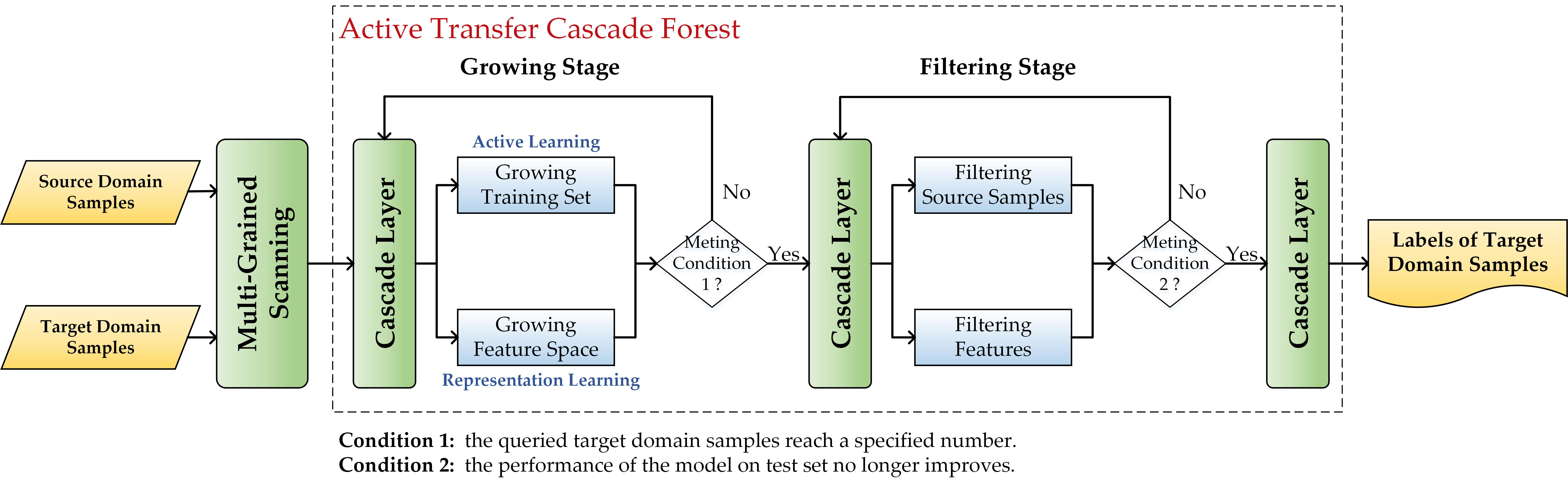
The key hypothesis of active learning is that if the learning algorithm is allowed to choose the data from which it learns to be “curious”, it will perform well with less training [28]. An active learning model includes a supervised predictive model (G), a training sample set (T), a query function (Q), an unlabeled sample set (U), a supervisor (S), and a queried sample set (L).
The main process of active learning is shown in Figure 1, where a set of highly informative labeled samples and a high-performance predictive model can be obtained at the end of the iteration. In brief, active learning is aimed at obtaining a small group of labeled samples that are the most informative, so as to construct a high-performance predictive model without using many labeled samples. Clearly, this can reduce the cost of querying adequate training samples, compared with random sampling and manual selection.
To obtain the most informative samples, it is necessary to accurately evaluate the informativeness of the unlabeled samples. Therefore, the key to active learning is to design an effective query strategy according to the specific data and task. Two commonly used query strategies are the uncertainty criterion and the diversity criterion.
The uncertainty criterion chooses the samples for labeling for which the model’s current predictions are least certain [29]. This criterion assumes that when the uncertainty of the sample is high, it carries information that is lacking in the current training set, and so adding the high uncertainty samples to the training set is helpful for improving the performance of the classifier. The most frequently used method to evaluate the uncertainty of samples is information entropy [29]. If we suppose that there are n possible classes of a sample, then its information entropy is calculated as follows:
where is the estimated probability of class .
We see from Equation (1) that when the prediction probabilities of all the classes are equal (), the information entropy of the sample reaches the maximum value (), and the classifier is completely unable to distinguish which class the sample belongs to. Thus, as the high-entropy samples tend to be close to the class boundary in the feature space, if the classifier can distinguish these samples correctly, it can effectively distinguish the other samples. That is to say, the uncertainty criterion is aimed at finding a set of samples with the highest entropy from the unlabeled sample set.
The diversity criterion involves choosing a group of samples that are different from each other, to avoid information redundancy of the samples. Here, we introduce two approaches to evaluate the diversity: cluster-based methods and methods based on the geometric spatial distance. (1) As clustering techniques are able to assign similar samples into the same cluster based on their distribution in the feature space, the clustering-based methods consider the selection of samples from different clusters to be effective in ensuring the differences between selected samples [30]. In addition, samples from different clusters are also somewhat representative of the distribution of the overall samples, so this approach can obtain a group of samples that are both diverse and representative. (2) The spatial distance-based methods evaluate the diversity via the distance of the samples in the feature space. The larger the distance, the greater the difference between samples.
A typical example of the spatial distance-based methods is the cosine angle distance [31], where the samples are first transformed into the kernel space, and then the cosine angle distance is calculated between the samples. For example, the cosine angle distance of sample and sample is as shown in Equation (2):
where is the nonlinear mapping function, and is the kernel function.
Researchers [22,30,32,33] have combined the uncertainty criterion and diversity criterion, aiming to select a set of samples with high uncertainty and diversity, to ensure that the information of these samples is rich enough. In this study, we also used both the uncertainty criterion and diversity criterion to select samples from the unlabeled target domain sample set, where the diversity criterion was redesigned based on the characteristics of the transfer learning task and the PolSAR data. This is described in detail below.
2.2. Deep Forest Model
Although deep neural networks are powerful, they do have some disadvantages, including being reliant on a large number of training samples, high complexity, and low interpretability. Furthermore, there are many hyperparameters in the deep neural networks, which typically require a great deal of effort to fine-tune. Zhou et al. [27] conjectured that if a suitable model was endowed with the representation learning capability of a deep neural network, the performance may be comparable to that of a deep neural network, while avoiding the above-mentioned shortcomings. Based on this conjecture, they proposed a deep forest model, which is a novel decision tree ensemble model that consists of multi-grained scanning and a cascade forest. The deep forest model is briefly described below.
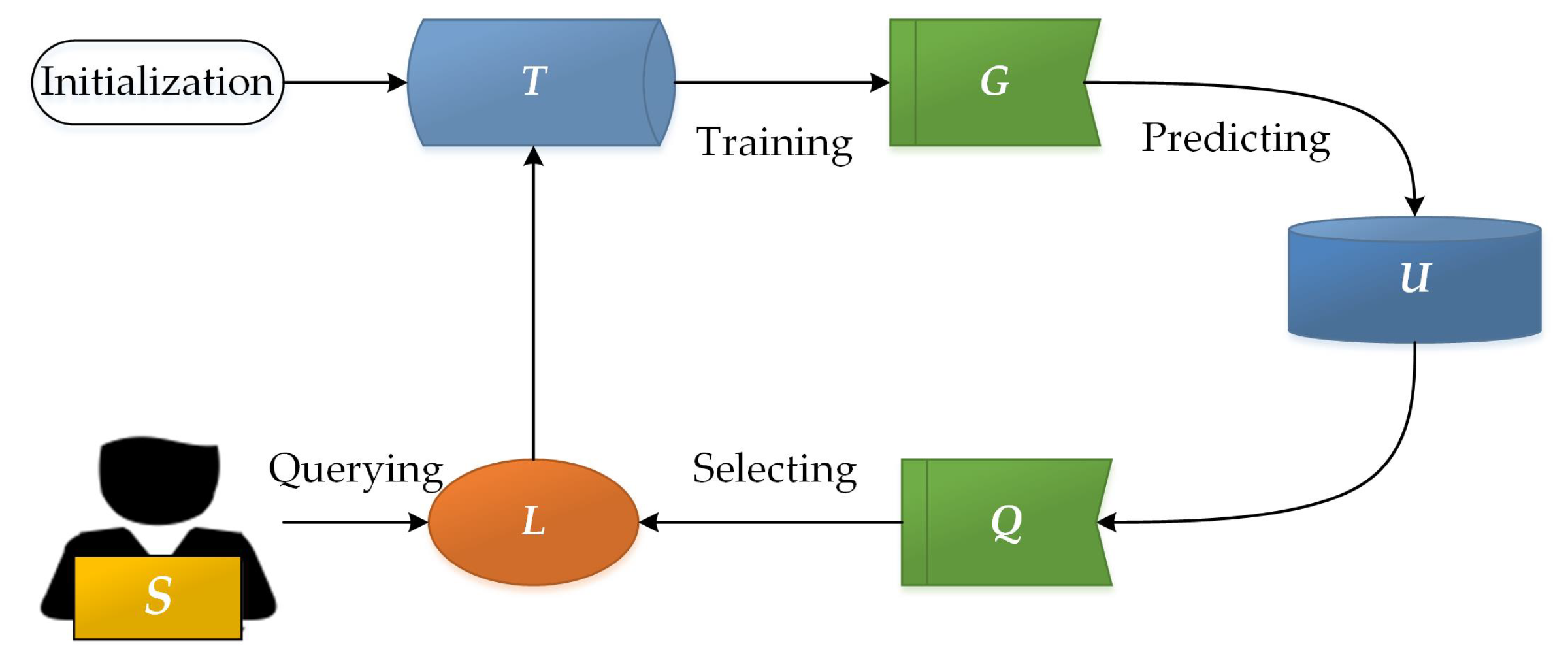
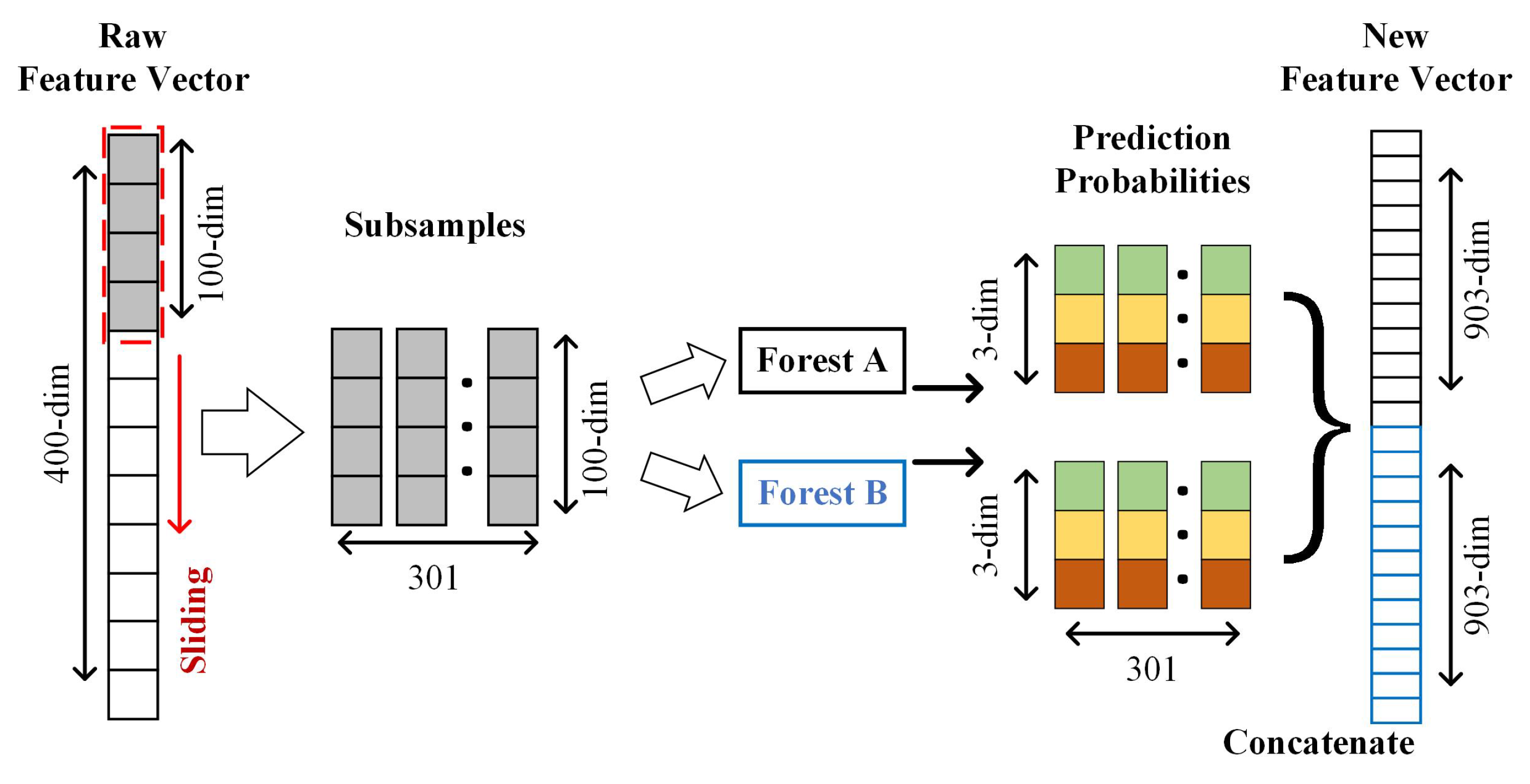
Multi-grained scanning is used to enhance the representation learning capability of the model. The flowchart of multi-grain scanning for sequence data is shown in Figure 2, in the case of there being 400 raw features and three classes. First, when the size of the sliding window is 100 and the sliding distance is 1, the model can obtain 301 subsamples (whose feature dimension is 100) by sliding one sample. Secondly, when a subsample is input into the random forest model, three estimated class probabilities can be obtained. Therefore, when 301 subsamples are input into two random forests, a total of () estimated class probabilities can be obtained. Finally, these estimated class probabilities are concatenated as transformed features (for the convenience of expression, they are called “multi-grained features” in this paper). In addition, using multiple sliding windows of different sizes for the multi-grained scanning can further increase the dimensionality of the multi-grained features. As each subsample represents a local feature of the raw sample, multi-grained scanning is equivalent to a structured up-sampling of the original feature, which enhances the representation learning capability of the model and helps to improve the performance.
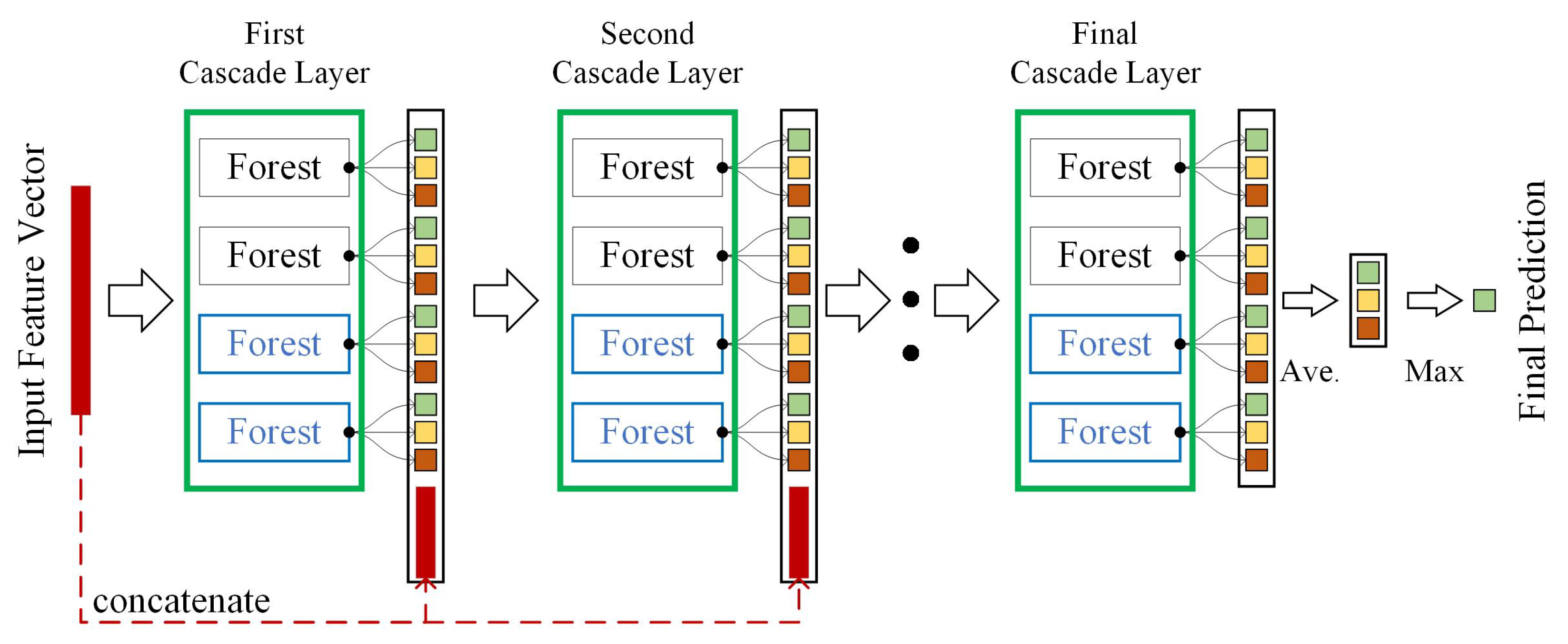
The representation learning capability of deep neural networks mostly relies on the layer-by-layer processing of the raw features. Inspired by this fact, the cascade forest model also employs a cascade structure, as shown in Figure 3. To encourage diversity, each level of the cascade forest includes two completely random tree forests and two random forests. For a sample, when the number of classes is three, these four random forests can output 12 estimated class probabilities as the augmented features of the sample. The augmented features are then concatenated with the multi-grained features to be used as the input features of the next level of the cascade forest.
In each level of the cascade forest, the training set is randomly split into two parts: the growing set is used to train the model, and the estimation set is used to estimate the performance of the model. If growing a new level does not improve the performance, the growth of the cascade terminates, which means that the model complexity can be automatically set. This also enables the model to avoid overfitting and perform well on different scales of data. The estimated class probabilities from the four random forests in the last cascade are averaged, and then the samples are assigned to the class labels with the highest estimated probabilities. For more information regarding the deep forest model, we refer the reader to [27]. Due to the deep forest model having the characteristics of a strong representation learning capability, fewer hyperparameters, strong interpretability of the model structure, and low computational cost, we constructed the proposed active transfer learning method based on the structure of the deep forest model.
2.3. The Proposed Active Transfer Learning Method
The task considered in this study can be defined as follows: for two PolSAR images (denoted by A and B) of the same region, there are a great deal of labeled samples in A, while B has no labeled samples. A is then taken as the source domain image, and its labeled samples are taken as the source domain samples (referred to as ). B is then taken as the target domain image, and a large number of unlabeled samples are randomly sampled from B as the target domain samples (referred to as ). The goal is to assign class labels to , without relying too heavily on manual labor.
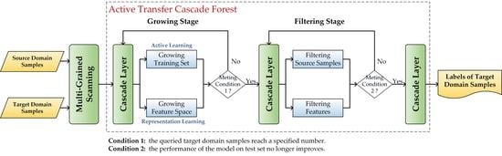
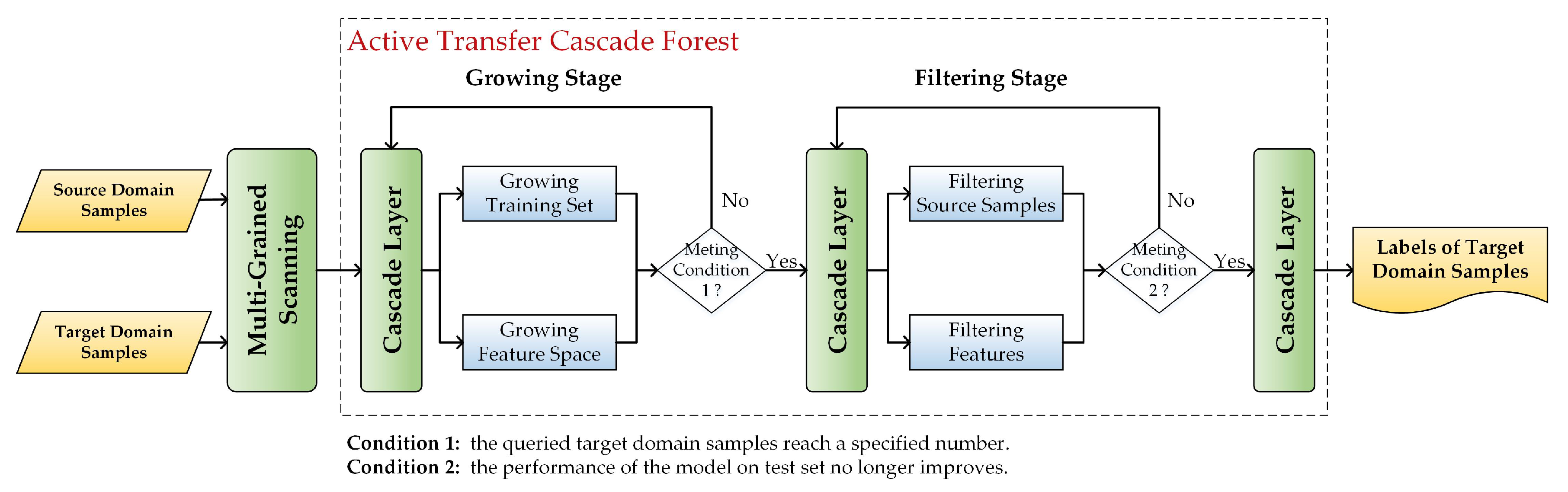
To achieve this goal, inductive transfer learning typically starts by querying a small group of samples from to use as the target domain labeled sample set (referred to as ), and then the label information of and is transferred to . As the quality of the samples is crucial to the transfer accuracy, the proposed method uses active learning to iteratively select the most informative unlabeled samples for labeling, to ensure that the information of the samples is sufficient. As the reduction of the distribution differences of the source and target domains helps to improve their transferability, the proposed method exploits the representation learning capability of the deep forest model to dynamically adjust the feature space to reduce the distribution differences of and . The main structure of the proposed method is shown in Figure 4.
The raw features of and are first transformed into multi-grained features by the multi-grained scanning forest (trained by ). The structure of the multi-grained scanning forest is consistent with that of the deep forest model, including a completely random tree forest and a random forest.
and are then input into the active transfer cascade forest, which consists of a growing stage and a filtering stage. In the growing stage, the performance of the model is gradually improved by updating the training set using active learning and adjusting the feature space using the augmented features. In the filtering stage, the performance is further improved by iterative processing until the model converges. At the same time, to accelerate the convergence of the model, two filtering strategies are used to remove the feature subspaces that are less helpful for the knowledge transfer and the source domain samples that do not fit with the distribution of the target domain samples. The class labels of are output from the final cascade layer. The growing stage and filtering stage are described in detail below.
2.3.1. Growing Stage
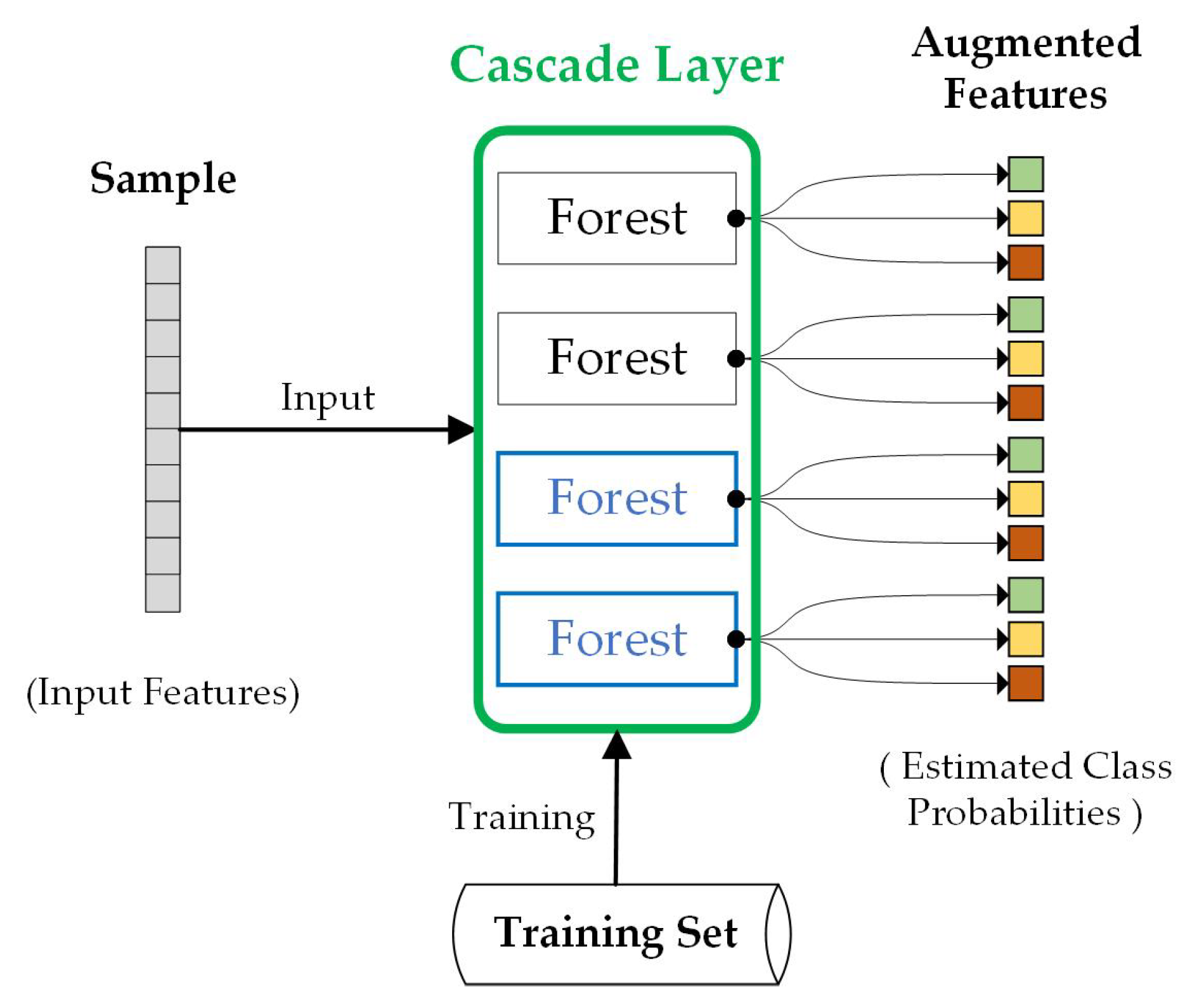
Figure 5 shows the relationship between the input sample, the training set, the cascade layer, and the augmented features, where the adjustments to the training set can change the performance of the cascade layer, thus affecting the quality of the augmented features of the input sample, which in turn affects the performance of the next cascade layer. Therefore, we designed the growing stage to iteratively grow the training set and feature space to improve the model’s performance on the target domain samples.
- The growth of the training set
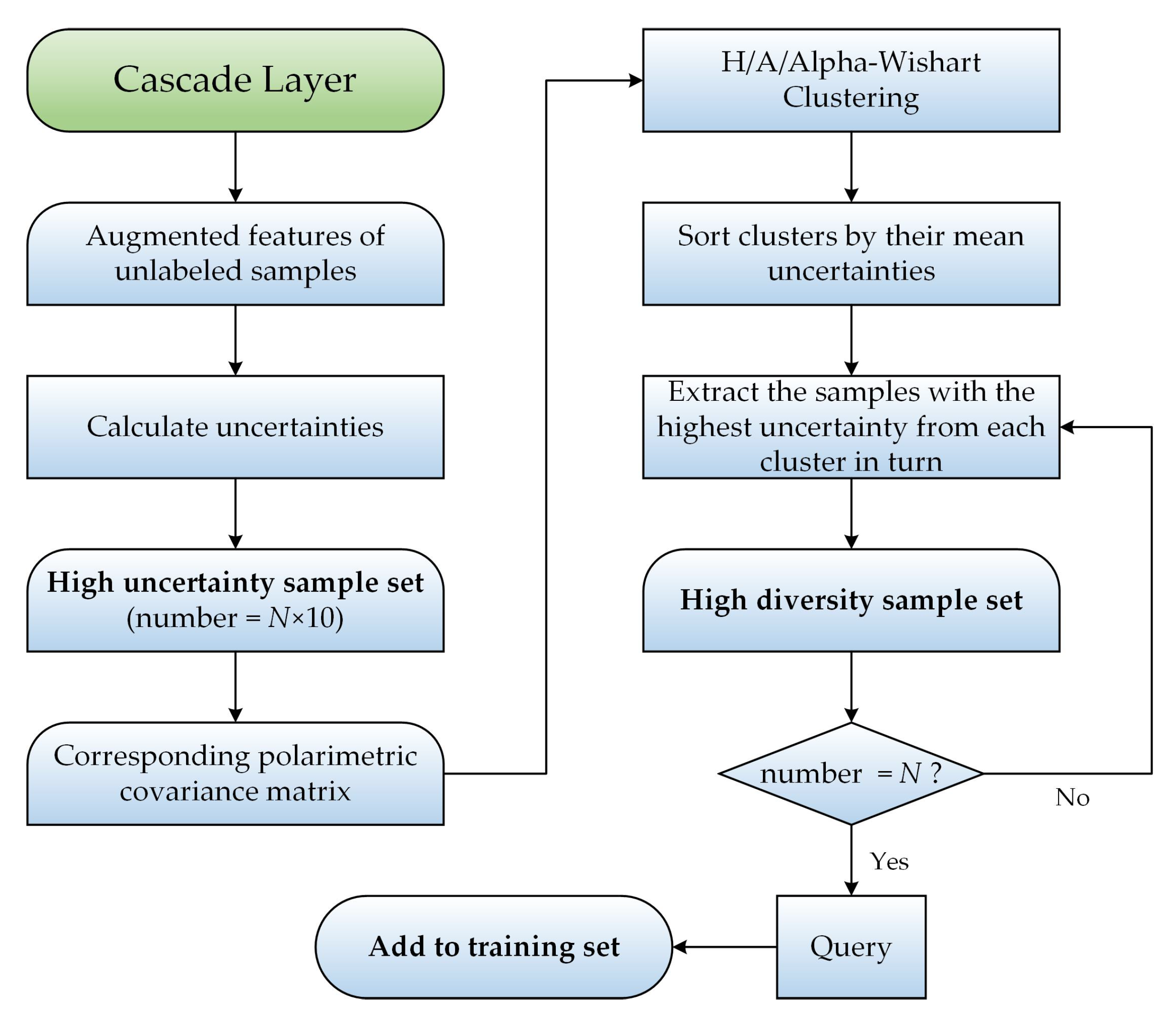
The aim of the growth of the training set is to add a limited number of target domain samples with rich information to the training set to improve the trained model’s performance in predicting the target domain samples. Informative samples are required to meet two conditions: (1) they should complement the knowledge that is lacking in the current training sets; and (2) there should be some divergence between these samples to avoid redundancy of knowledge and to maintain the balance of classes, i.e., the informative samples are a set of samples with high uncertainty and sufficient diversity. Clearly, neither random sampling from the sample set nor manual selection can guarantee that the selected samples satisfy these conditions; thus, active learning is needed. To extract the informative samples from the target domain sample set accurately, according to the characteristics of the transfer learning task and PolSAR data, we designed a new active learning strategy that considers the uncertainty and diversity. The flowchart of the new active learning strategy is shown in Figure 6.
The growing stage is iterative, assuming that in one iteration, we want to select the N most informative samples from the target domain unlabeled sample set () to add to the training set. The detailed procedure of the proposed active learning strategy is as follows:
The first step is to obtain the samples with the highest uncertainty from as the high uncertainty sample set. As mentioned in Section 2.1, one of the most effective ways of evaluating the uncertainty of samples is to calculate the information entropy through the estimated class probabilities. As the augmented features of each sample under the current cascade layer are their estimated class probabilities, we do not need to train an additional classifier to estimate the sample’s class probabilities, but rather we can quickly compute its information entropy directly from the augmented features.
The second step is to select the N samples with sufficient diversity from the high uncertainty sample set as the highly informative sample set. For the measurement of the diversity of the target domain samples, the conventional methods (as mentioned in Section 2.1) are designed for classification tasks in which the training set and test set usually come from the same domain so that they can accurately measure the diversity of the samples of the test set in the current feature space. However, in the transfer learning task (where the data distributions of the training set and test set are different), the feature space may be unstable due to its transition from source domain to target domain, and thus the measurement of the diversity of the target domain samples in the current feature space may be inaccurate.
To accurately select a set of target domain samples with great diversity, based on the characteristics of PolSAR data, we designed the following sample selection approach, which is independent of the current feature space: (1) use H/A/Alpha-Wishart clustering [34] to divide the high uncertainty sample set into up to 16 clusters based on their polarimetric covariance matrices (); (2) calculate the means of the uncertainties of all the samples in each cluster, and then sort all the clusters according to their mean uncertainty values from large to small; and (3) extract samples with the highest uncertainty from each cluster in ranked order, until the number of extracted samples is equal to N.
The final step is to manually assign class labels to the extracted samples, and then a set of target domain labeled samples with the highest uncertainty and sufficient diversity is obtained. These are then added to the training set with weights set to twice the size of the source domain samples.
The proposed active learning strategy has the following advantages. First, the samples are clustered according to their backscattering properties using H/A/Alpha-Wishart clustering, where the clusters represent different scattering characteristics, so extracting samples from the different clusters can guarantee their diversity. Secondly, the clustering only uses the polarimetric covariance matrices of the target domain samples, and is independent of the current multi-grained features and the source domain samples and, thereby, is more effective than the conventional methods. Thirdly, a higher mean uncertainty for the cluster indicates that the knowledge of the scattering type represented by the cluster is relatively lacking in the current training set, and so selecting samples from clusters with higher mean uncertainty can ensure that the selected samples are sufficiently informative. Finally, the distribution of the clusters reflects the distribution of ; thus, the selected samples from different clusters are also representative of , to an extent, which can help the adaptive convergence of the model in the filtering stage (as described in Section 2.3.2).
- The growth of feature space
Many of the feature-based transfer learning methods attempt to find domain-invariant features as the domain difference can be dramatically reduced when represented by these features, which allows the models trained on source domain data to perform well on target domain data [35]. Inspired by this, the aim of the growth of the feature space is to exploit the representation learning capability of the cascade forests to generate augmented features, which have great representational ability across domains, to gradually adjust the feature space and improve the transferability of the source and target domains.
As some of the highly informative target domain samples are added to the training set in the growth of the training set, the augmented features generated by the combined training set will have a better cross-domain representational ability than the original multi-grained features, i.e., when represented by the augmented features, the difference across domains should be reduced. Based on this assumption, if sufficient augmented features are added to the feature space, the transferability of the source and target domains in the grown feature space will be improved. Therefore, when iteratively expanding new cascade layers with the growth of the training set, the augmented features are concatenated with the multi-grained features simultaneously to gradually enhance the transferability across domains, thus, improving the performance of the model on the target domain samples.
More specifically, for a cascade layer of the proposed method, the input features are equal to the multi-grained features plus all of the augmented features generated by the previous cascade layers (whereas in deep forest, the input features are equal to the multi-grained features plus the augmented features of the last cascade layer). In addition, the reduction of the distribution difference can improve the transferability, and, thus, one reason the growth of the feature space is effective is that it reduces the distribution difference between the source domain samples and the target domain samples (which was proved in the subsequent experiments).
2.3.2. Filtering Stage
When the target domain labeled samples () reach a specified number, the model moves from the growing stage to the filtering stage, where the iterations are continued to expand to new levels of the cascade layers to further improve the performance of the model until the model converges. The reason for this is that the number of samples reaches the maximum in the last cascade layer of the growing stage; thereby, the continuous iterations are able to fully exploit the knowledge of these highly informative samples to enhance the model, as well as further adjust the feature space using the augmented features. When the model converges, continuing the iterations will not improve the performance of the model, and the newly generated augmented features will be redundant; thus, it is important to terminate the iteration at this point.
For the stopping criterion, deep forest uses a set of samples randomly divided from the training set to evaluate the performance of the model, and the model is considered to be converged when the performance no longer improves. As the labeled and unlabeled samples in the classification task typically come from the same domain, the above stopping criterion is effective in the classification task. However, the source and target domain samples in the transfer learning task come from different domains and have different data distributions; therefore, the above stopping criterion is unsuitable for evaluating the model’s performance on target domain samples.
To accurately judge whether the model is converged, considering that was obtained by the proposed active learning strategy, and is highly informative and representative for the target domain unlabeled samples (), we consider that if the model has a good prediction effect on , the model will also have reliable performance in predicting . Therefore, the stopping criterion of the proposed method is set as follows: the iteration of the filtering stage stops if the model’s prediction accuracy on no longer improves. The use of this stopping criterion allows automatic control of the iteration of the model and allows us to adaptively adjust the depth of the cascade forest. It can also reduce the risk of overfitting, and makes the model adaptable to different scales of data.
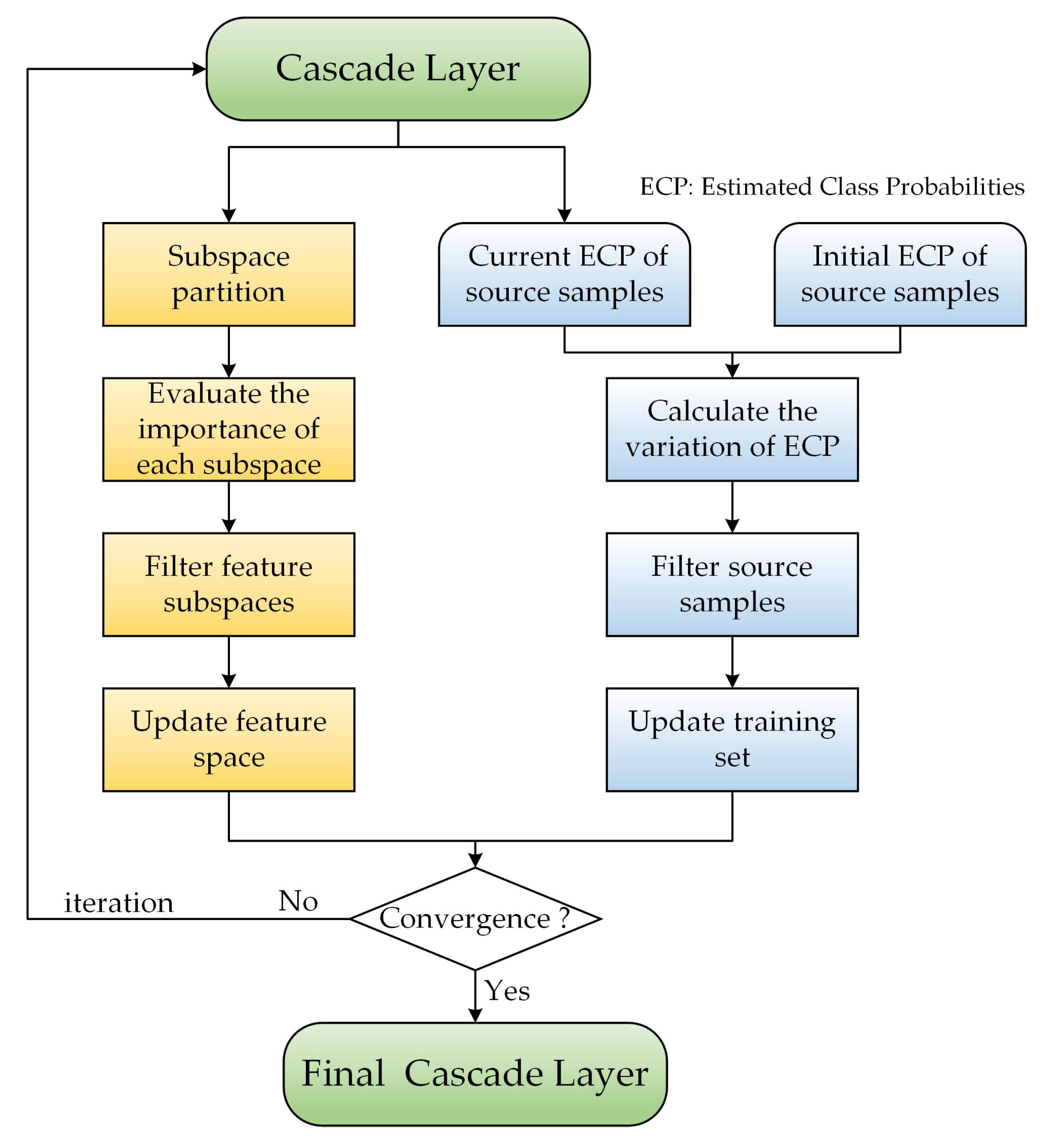
In addition, to accelerate the convergence of the model, we considered two common problems in transfer learning. (1) Not all the features are useful for the transfer, and some cause the differences across domains. If we can identify and remove these domain-sensitive features (the opposite to domain-invariant features), the interdomain discrepancy in distributions should be reduced. (2) Some of the source domain samples that are quite different from the distribution of the target domain samples may lead to the negative transfer effect. Therefore, in the filtering stage, benefiting from the cascade structure of the proposed method, we can iteratively filter the feature subspace and source domain samples with the expansion of the cascade layers to accelerate the convergence of the model. The flowchart of the filtering stage is shown in Figure 7.
- Feature subspace filtering
In the removal of the domain-sensitive features, considering the discriminative ability of the features is necessary to avoid reducing the class separability by the removal of discriminative features. That is to say, in feature subspace filtering, we filter out the feature subspaces that are domain-sensitive and have a low discriminative ability. The procedure of feature subspace filtering is shown in flowchart form in Figure 7.
First, the whole feature space is divided into many feature subspaces, as it is inaccurate to estimate the distribution of source and target domain samples in a single dimension of features, and this is also able to improve the computational efficiency. When partitioning the feature space, the dimensions of each feature subspace are consistent with the dimensions of the augmented features generated by a single cascade layer: if the number of classes of samples is , then the dimension of each feature subspace will be ; thus, a feature space with dimension D will be randomly divided into () feature subspaces.
Secondly, divergence between domains (denoted by DBD) is used to evaluate the domain sensitivity of each feature subspace, which is calculated as follows [36]: for the source domain samples () and target domain samples (), these samples are first combined together, regardless of their true labels, with as positive samples with pseudo label 1 and as negative samples with pseudo label 0. A linear classifier is then used to perform k-fold cross-validation on these samples in the feature subspace, and the overall accuracy of the cross-validation is taken as the DBD of the feature subspace. The higher the DBD, the more sensitive the feature subspace is to the shift between domains.
The discriminative ability of the feature subspaces is then evaluated. Feature importance is used to measure the discriminative ability, where the greater the feature importance of a feature subspace, the more important it is to maintain the class separability. Therefore, we first output the feature importance of each feature through the random forests in the cascade layer, and then, for each feature subspace, the sum of the feature importance of all the features within that subspace is used as its subspace feature importance (denoted by SFI) for measuring the importance of that subspace in maintaining class separability. The higher the SFI, the greater the feature importance of the feature subspace.
Finally, the feature subspaces with high DBD and low SFI are removed from the feature space, i.e., the feature subspaces with the highest value of () are removed. The removal of the feature subspaces that are domain-sensitive and non-discriminative can improve the transferability of the knowledge between the source and target domains. However, the values of DBD and SFI must be normalized before processing.
- Source domain sample filtering
Negative transfer is typically due to dissimilarity between source domain and target domain data, and thus the purpose of the source domain sample filtering is to remove the source domain samples that do not match the distribution of the target domain samples to reduce the negative transfer effect. This strategy has also been a commonly used source domain sample filtering method in the recent related studies. For example, Deng et al. [22] filtered the source domain samples by determining how much the class conditional probability density of the source domain samples changed during the transfer process. If the class conditional probability density of a sample varies significantly, this indicates that the sample does not fit with the distribution of the classes in the target domain, and therefore needs to be removed from the training set.
Inspired by the previous studies, in the proposed approach, the source domain samples are filtered according to the change degree of their estimated class probabilities. We use a source domain sample X with three possible classes () as an example. First, the estimated class probabilities of the samples output from the first level of the cascade layers in the growing stage are taken as the initial estimated class probabilities . The current estimated class probabilities are then output from the last level of the cascade layers in the filtering stage. Finally, assuming that and are the two classes with the highest probability in , the degree of change of the estimated class probability is calculated by Equation (3).
where
If is greater than the threshold (which is an “experience threshold”), the source domain sample will be removed from the training set. As the first cascade layer has not yet added the target domain samples to the training set, while the subsequent cascade layers adjust both the training set and the feature space and make the distribution of the training set transition from the source to target domain gradually, if the estimated class probability of a source domain sample is considered to be stable, it is considered to fit with the distribution of the classes in the target domain. Conversely, those source domain samples with significant changes in the estimated class probabilities should be removed.
When the model converges, the estimated class probabilities of output from the four random forests in the final cascade layer are averaged, and then the classes with the highest probabilities are taken as the prediction result of the target domain samples, so that the class labels of all the target domain samples can be obtained. The detailed processing flow of the proposed method is presented in Algorithm 1.
| Algorithm 1: Proposed active transfer learning method. |
| Input: source domain samples (), target domain samples (). |
| Output: class labels of . |
| Require: active learning strategy (), filtering criterion of (), |
| filtering criterion of feature subspaces (). |
| Begin: |
| 1: train multi-grained scanning forest based on . |
| 2: transform and from raw features into multi-grained features. |
| 3: initialize: target domain labeled samples . |
| Repeat until the number of meets the requirements |
| 4: train cascade layer based on . |
| 5: generate augmented features for all the samples and concatenate with multi-grained features. |
| 6: use to select N samples from for manual annotation, and then add them to . |
| End repeat |
| Repeat until performance of the model no longer improves |
| 7: train cascade layer based on . |
| 8: generate augmented features for all the samples and concatenate with multi-grained features. |
| 9: use to remove domain-sensitive feature subspaces. |
| 10: use to remove samples from . |
| 11: evaluate the performance of the model based on the classification accuracy of . |
| End repeat |
| 12: obtain the class labels of from the final cascade layer. |
3. Experiments
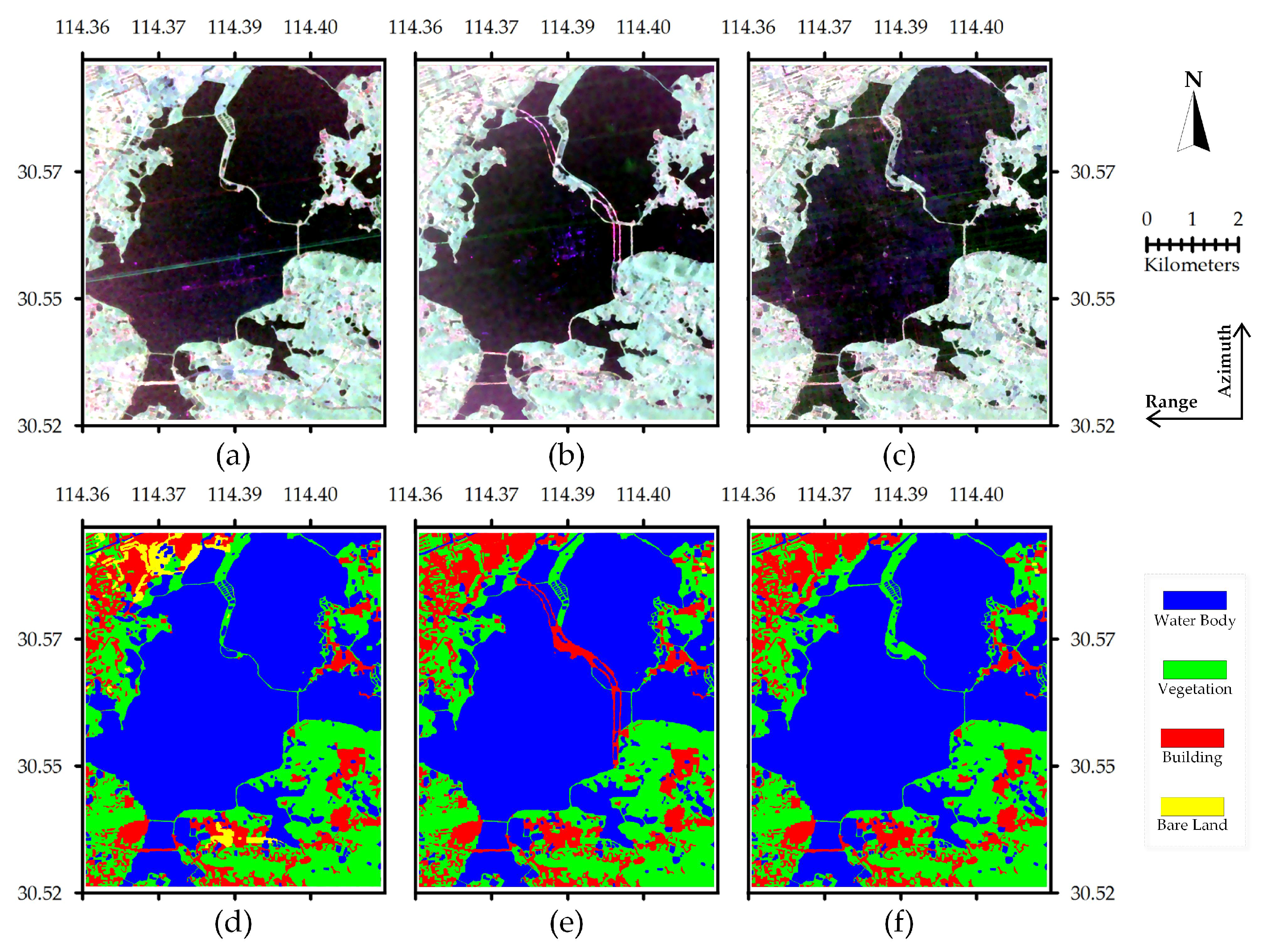
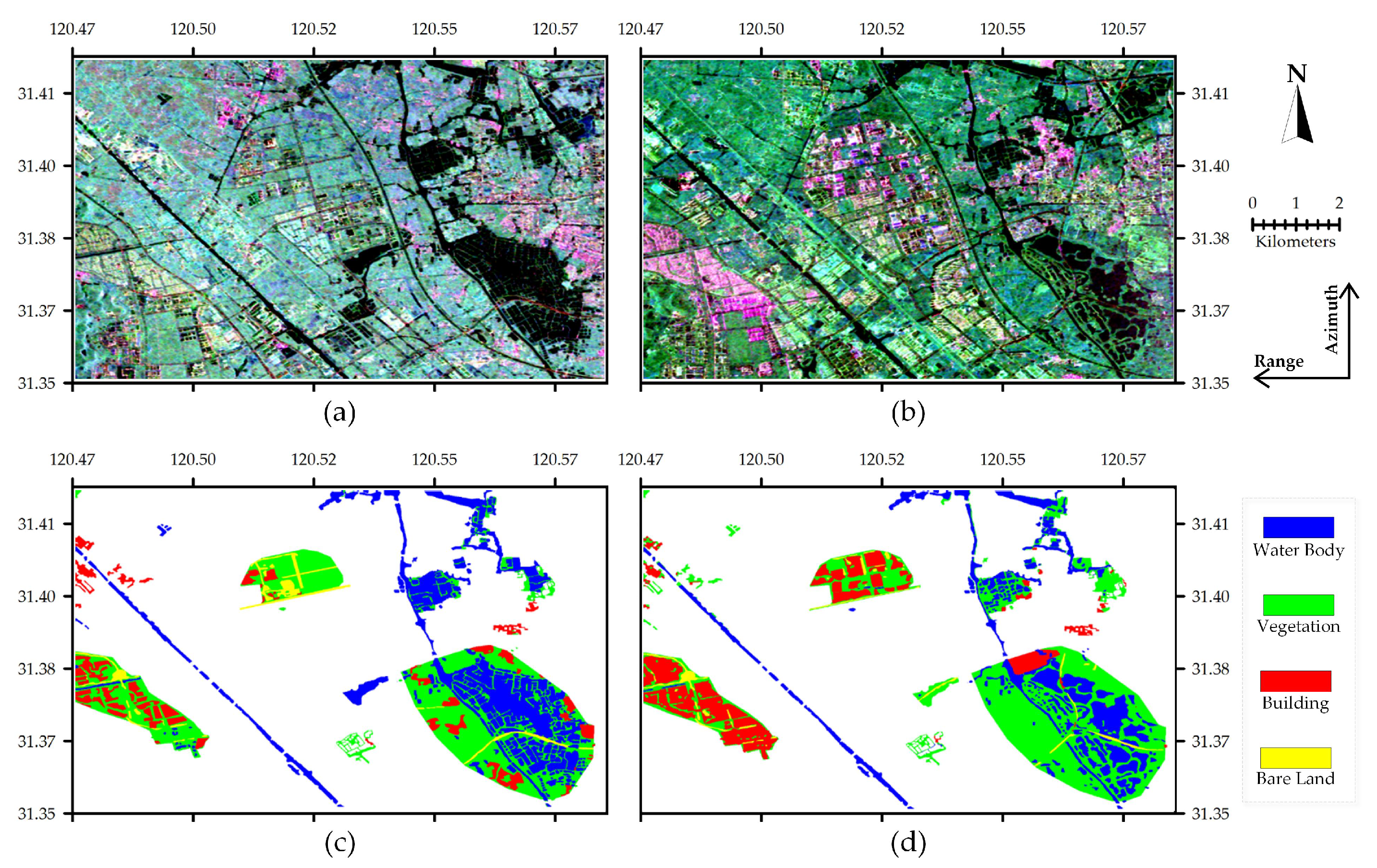
To evaluate the performance of the proposed method, a total of five PolSAR images obtained by the RADARSAT-2 (RD-2) and Gaofen-3 (GF-3) sensors were used for the experiments, and four state-of-the-art transfer learning methods were used for the comparison. The Pauli-RGB images ( for red (R), for green (G), and for blue (B)) and ground-truth maps of these PolSAR images are shown in Figure 8 and Figure 9. The ground-truth maps were obtained by the visual interpretation of the images, and to improve the reliability, we used the online optical image map as the reference data. All the experiments were performed on a 64-bit Windows 10 PC, and the programming language used to implement the algorithms was Python 3.
3.1. Experimental Data and Settings
The three images in Figure 8 are fully polarimetric SAR images of Wuhan, Hubei province, China, each with the same size of pixels, and the main classes of ground objects were water, vegetation, and buildings (bare soil only exists in the first image; thus, it is not considered). The two images in Figure 9 are fully polarimetric SAR images of Suzhou, Jiangsu province, China, with the same image size of pixels. Due to the difficulty of labeling the ground-truth maps, only a portion of this area was used for the experiments (the non-white areas in Figure 9a,b), and the main classes of ground objects were water, vegetation, buildings, and bare soil. Based on the above five PolSAR images, three set of experiments were conducted.
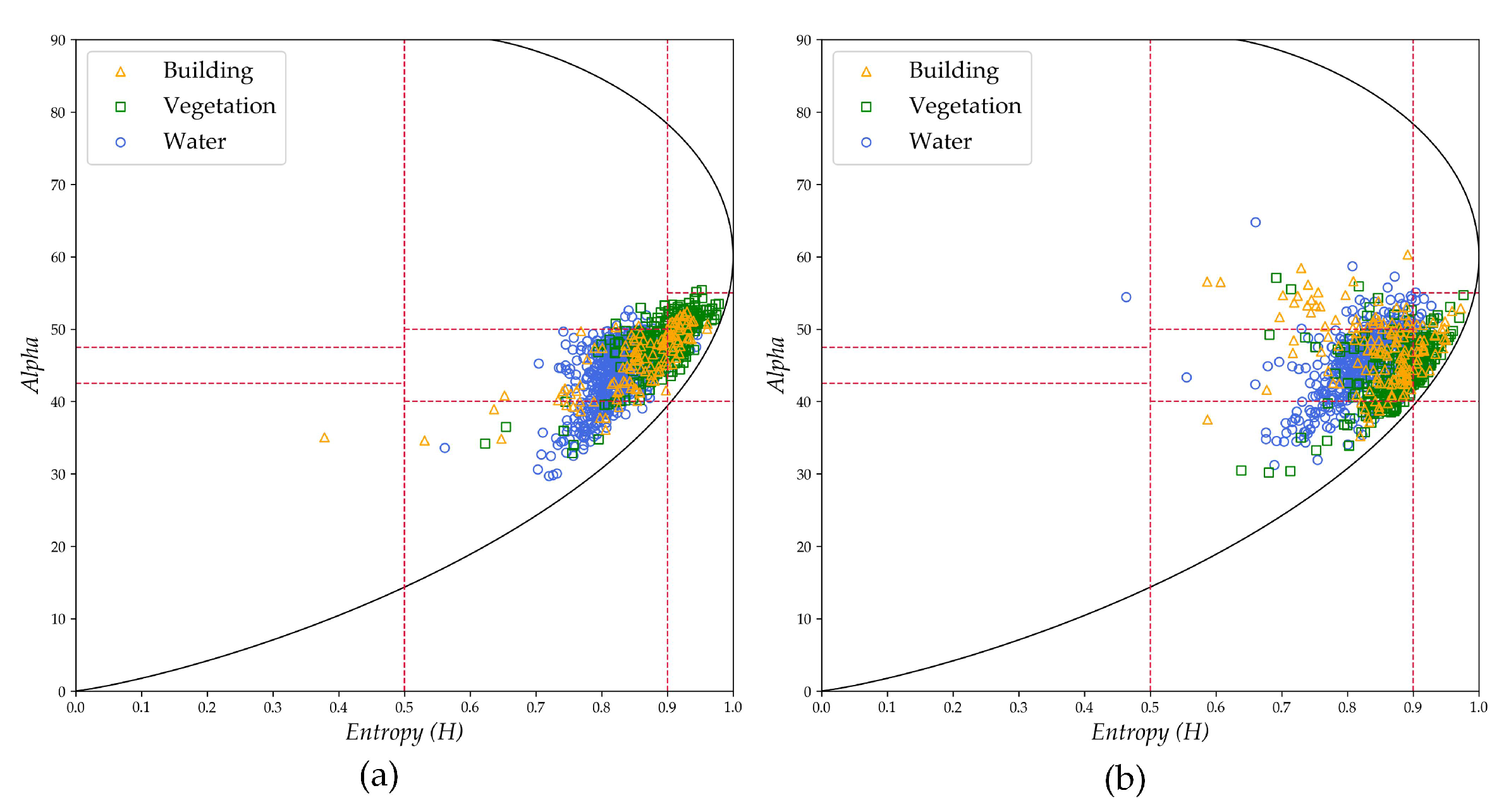
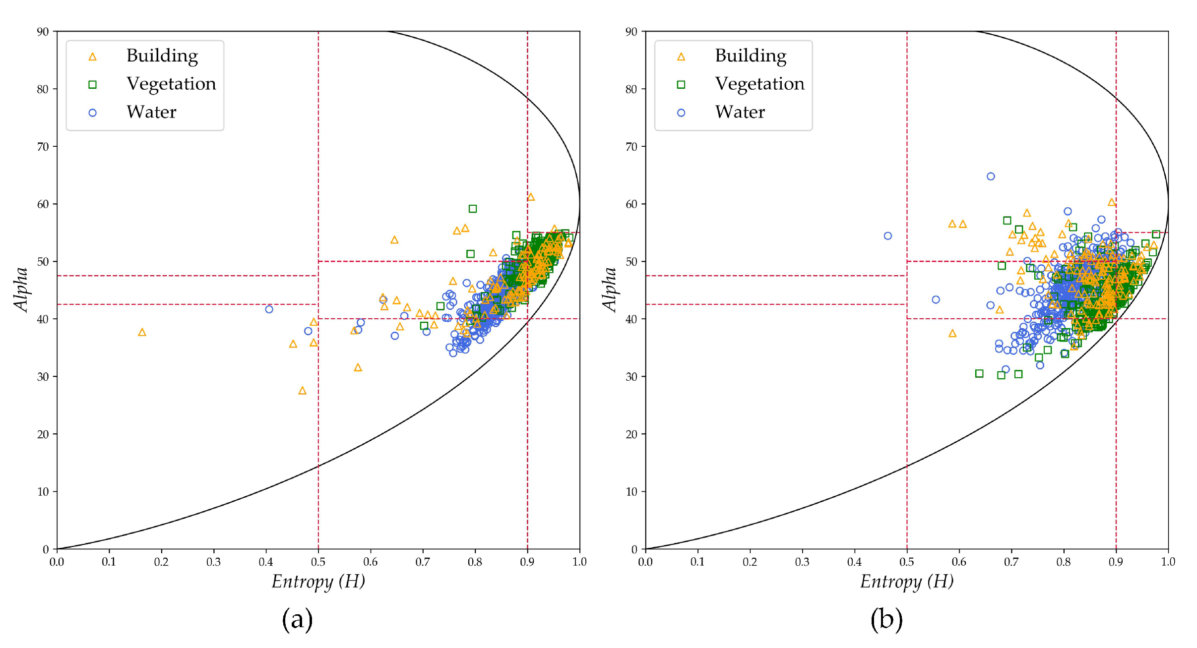
(1) The first set of experiments involved the images of Wuhan, with the 2011 image as the source domain and the 2017 image as the target domain. This set of experiments was aimed at verifying the knowledge transfer capability of the transfer learning method between images with a large imaging time span and from different sensors (RD-2 to GF-3). The distributions of the used source domain samples and target domain samples in the H-Alpha plane are shown in Figure 10. The H-Alpha plane is a commonly used feature space in PolSAR image processing for visualizing the sample distribution, with each region of the plane corresponding to a specific type of backscattering, as detailed in [34].
(2) The second set of experiments involved the images of Wuhan, with the 2016 image as the source domain and the 2017 image as the target domain. This set of experiments was aimed at verifying the knowledge transfer capability of the transfer learning method between images with a small imaging time span and from different sensors (RD-2 to GF-3). The distributions of the used source domain samples and target domain samples in the H-Alpha plane are shown in Figure 11. The target domain in this set of experiments was the same as that in the first set of experiments, and the distribution difference in Figure 11 is smaller than that in Figure 10. A smaller distribution difference typically indicates better transferability. Therefore, the transfer effects of these two sets of experiments were compared with each other in the following.
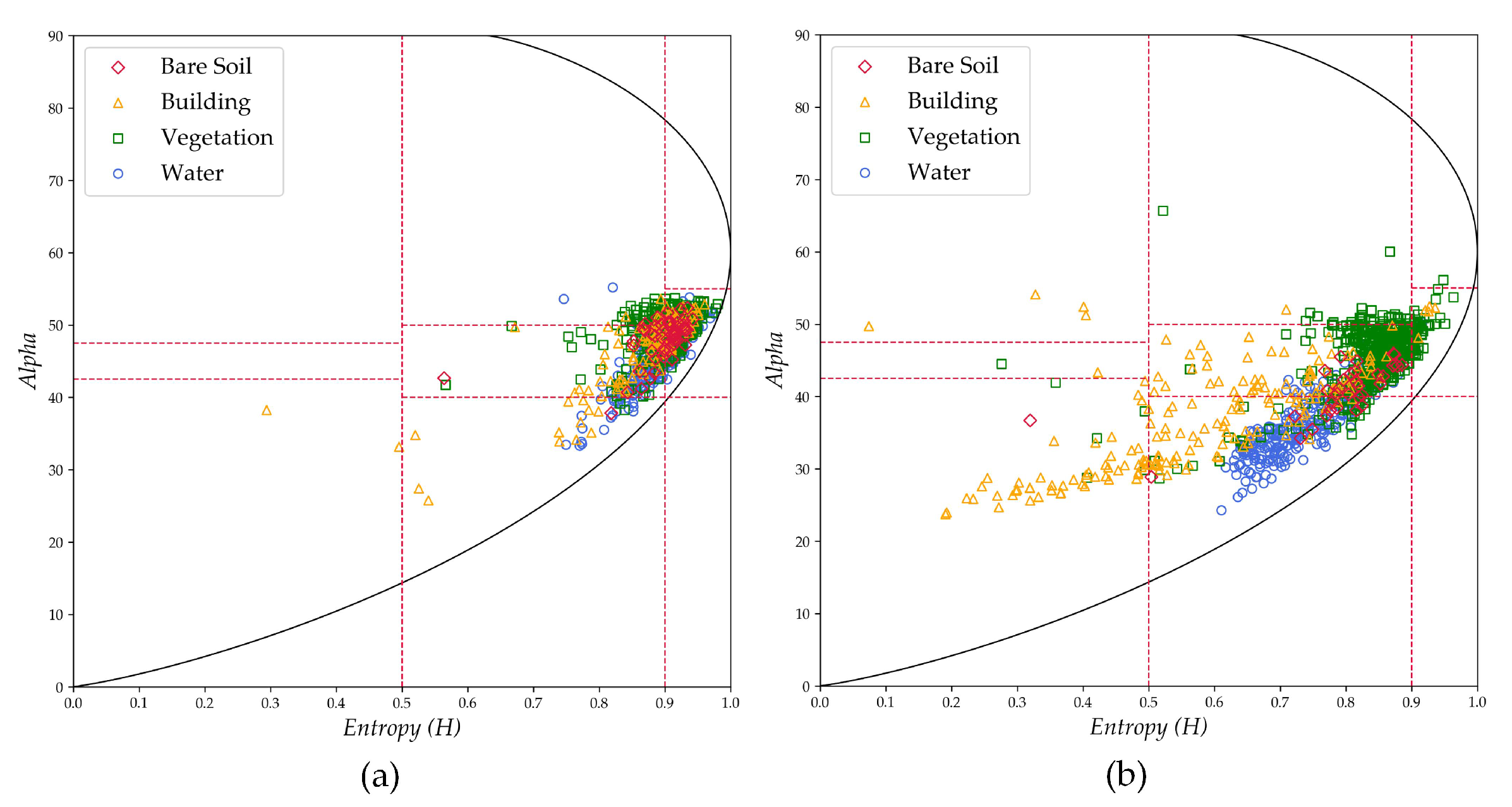
(3) The third set of experiments involved the images of Suzhou, with the 2008 image as the source domain and the 2016 image as the target domain. This set of experiments was aimed at verifying the knowledge transfer capability of the transfer learning method between images with a large imaging time span and from the same sensor (RD-2 to RD-2). The distributions of the used source domain samples and target domain samples in the H-Alpha plane are shown in Figure 12. Due to the long imaging time span and the rapid economic development of this area, there were not only changes of the classes of ground objects between the two images, but also great differences in the same classes of ground objects, such as low-rise buildings becoming high-rise buildings, open water being divided into small areas of water, etc. Although the classes of the objects were not changed, the polarization characteristics of the objects were changed, causing the same class of objects to display different backscattering properties (the corresponding Pauli RGB images shown in Figure 9 also attest to this problem). Hence, the distribution differences of this group of experimental data are relatively large.
To avoid randomness, each set of experiments was repeated 10 times, and the mean value was used as the final result. In each experiment, 1000 source domain samples and 1000 target domain samples were randomly sampled from the source and target domain images, respectively. As the performance of inductive transfer learning is related to the amount of information contained in the target domain labeled samples (), and the greater the number of , the more information it is able to carry, we set up an incremental number sequence of : to evaluate the reliability and stability of the transfer learning method under different numbers of . For the performance evaluation criterion, the overall accuracy of the model for all the target domain samples was taken as the transfer accuracy.
In the experiments, a total of 35 features were used as the raw features of the samples, including nine features extracted from the polarimetric coherence matrix and 26 features obtained from several polarimetric decomposition methods. These polarimetric decomposition methods were: H/A/Alpha decomposition, Van Zyl three-component decomposition, Yamaguchi four-component decomposition, Arii three-component nonnegative eigenvalue decomposition (NNED), An and Yang four-component decomposition, L. Zhang five-component decomposition, and Singh four-component decomposition.
3.2. Comparison with Existing Methods
The proposed method is an inductive transfer learning method, and thus four existing inductive transfer learning methods and a baseline method were used for comparison in the experiments. The comparison methods were as follows:
As all of the above five methods require a classification model as the weak classifier or the final classifier, Support Vector Machine (SVM) with radial basis function (RBF) kernel was chosen according to the relevant literature and our experimental analysis. To improve the performance of each weak classifier, a grid search strategy and k-fold cross-validation (K-CV) were used to determine the optimal model parameters (“C” and “”) of the RBF kernel SVM, where “C” is the regularization parameter with its grid values set to , and “” is the kernel coefficient for the RBF kernel with its grid values set to . The value of k for the K-CV was set to 3. In addition, the initial input data of the above four transfer learning methods were , , and , while the initial input data of the proposed method were only and , as the samples of the proposed method were iteratively selected from during the processing.
According to “what to transfer”, BETL and TrBagg are instance-based transfer learning methods, and one of the main strategies for this type of method is to reweight based on the knowledge of , making the source domain samples that contribute to the transfer have a greater impact on the model; therefore, the transfer effects of such methods are subject to the informativeness of . SMIDA and SSTCA are feature-based transfer learning methods that mainly attempt to find the domain-invariant features, and they can also perform transfer in the absence of samples, and thus their transfer effects are less sensitive to the number of . The sensitivity of the proposed method to the number of lies between the above-mentioned two types of methods.
The mean and standard deviation of the transfer accuracies of the transfer learning methods under different numbers of samples were used for the comparison and analysis in the experiments. As the Baseline method only uses as the training set, its accuracy is independent of the number of ; therefore, its accuracy was used as a benchmark in the experiments to evaluate the negative transfer effect of the transfer learning methods, i.e., when the transfer accuracy of a method is lower than the Baseline method, this indicates that there is a negative transfer effect in the method.
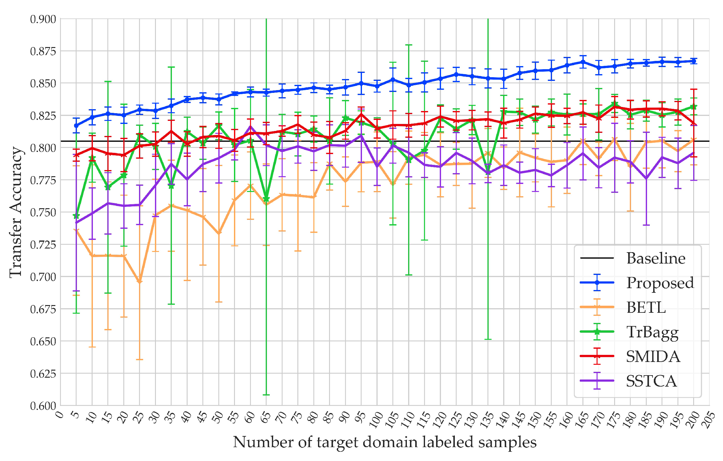
Figure 13 shows the results of the first set of experiments. Overall, except for SSTCA, the transfer accuracies of the other methods improved with the increase of the number of samples. BETL and TrBagg are more unstable than the other methods due to their high sensitivity to the quality of the samples. The accuracy of SMIDA was high when the number of samples was small, and the accuracy curve was stable with the increase of the number of . The proposed method also achieved a high accuracy, and was as stable as SMIDA. On the other hand, the accuracy of SSTCA decreased from 81.63% to 77.6% when the size of exceeded 60.
When the samples reached a certain number, only BETL and SSTCA showed significant negative transfer effects. The reason for the negative transfer effect of BETL is that it is an ensemble model of weak classifiers trained by subsets of , and when the distribution difference between the two domains is large, the performance of the weak classifiers is poor, causing the poor performance of the ensemble model. The points where SSTCA exhibited a negative transfer effect are consistent with the points of its accuracy decline, and one of the potential causes is that when the distribution difference between the two domains is large, adding a large number of samples to the training set causes two different data distributions to exist in the new training set, resulting in SSTCA being unable to maintain the local geometry of the data (which is crucial to maintaining the class separability of the samples), thus, reducing the model performance.
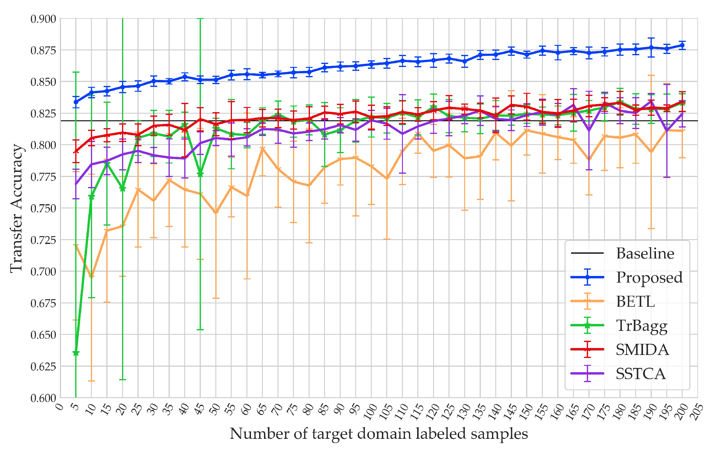
Figure 14 shows the results of the second set of experiments. The imaging time span between source image and target image was smaller than that in the first set of experiments; thus, the distribution difference was less, and it can be found that the transfer accuracies of all the methods in this set of experiments were better than in the first set of experiments. For instance, the accuracies of the Baseline method in the first and second experiments were 0.805 and 0.819, respectively.
With the increase of the number of samples, the accuracy curves of BETL, TrBagg, SMIDA, and SSTCA tended to approach the maximum faster than in the first set of experiments. The reason for this is that the lower the distribution difference, the fewer samples are needed to supplement the lack of knowledge of . That is to say, in this set of experiments, the newly added samples were more likely to be redundant samples (that are unhelpful for improving the transfer accuracy) when there are already many samples in the training set.
In the first two sets of experiments, the proposed method obtained a high accuracy (81.71–87.87%) and a low standard deviation, which is competitive to the results of the other methods (63.57–83.42%). (1) When the number of samples was small, the accuracies of the other methods were lower than that of the Baseline method, while the accuracy of the proposed method was higher than that of the Baseline method. As the active learning strategy of the proposed method can select the samples that are the most helpful for the transfer learning, the accuracy was relatively high. The samples of the other methods were obtained by random sampling; therefore, their informativeness was unstable, in particular when the number of samples was small. (2) With the increase of the number of samples, the accuracy of the proposed method was continually improved, as the active learning strategy of the proposed method was able to ensure that each newly added sample was informative to the current training set, thus, avoiding information overlap.
The first two sets of experiments proved that the proposed method was able to perform well in knowledge transfer between RD-2 and GF-3 images with both a large imaging time span (2011–2017) and a small imaging time span (2016–2017).
Figure 15 shows the results of the third set of experiments. In general, the variation trends of the accuracy curves of the transfer learning methods were similar to those in the first two sets of experiments. However, as the distribution difference was greater, the accuracy of the Baseline method was only 58.4%, which is significantly lower than that in the first two sets of experiments. Thus, when , the results of all the transfer learning methods were over 65.73%, indicating a positive transfer effect compared to the Baseline method. In addition, the accuracy curves of BETL and TrBagg tended to approach the maximum when , which further proves the assumption presented in the second set of experiments, i.e., the greater the domain difference, the more samples are required to supplement the lack of knowledge of .
Due to the large distribution difference, when the number of samples was small, the information provided was very limited in improving the transfer accuracy. Therefore, when , the accuracies of BETL, TrBagg and the proposed method were less than 58.34%, while SMIDA still achieved a high accuracy of 77.02%, due to its insensitivity to the quality of the samples. The accuracy curve of the proposed method ascended rapidly from 63.69% to 80.32% when , and when , the accuracy of the proposed method increased from 81.90% to 88.76%, whereas the maximum accuracy of the other methods was only 83.55%. The results demonstrated the effectiveness and reliability of the proposed method in knowledge transfer between images with a large imaging time span (2008–2016).
The results of the three sets of experiments are summarized in Table 1. Both SMIDA and the proposed method achieved high accuracies and low standard deviations, whereas the accuracy of BETL was relatively low, and the stability of TrBagg was poor. In addition, the average computational time of different methods in the three sets of experiments are presented at the end of Table 1. The proposed method required more computational time than the other methods. One of the main reasons is that the 35-dimensional input features were transformed into 684-dimensional multi-grained features in the multi-grained scanning of the proposed method, which increased the computational cost. Another reason is the number of iterations, and this will be described in detail in Section 3.3.2.
From the three sets of experiments, we can make the following conclusions: the instance-based transfer learning methods (BETL and TrBagg) can make full use of the knowledge of the samples; thus, their accuracies improve rapidly with the increase of the number of samples, whereas their accuracies also suffer from the unstable quality of the samples, and so the standard deviation of their accuracies is relatively high. The feature-based transfer learning methods (SMIDA and SSTCA) can reduce the distribution difference between the source and target domains by adjusting the feature space; therefore, their accuracies are more stable, and they can achieve high accuracies even when the number of samples is small. The proposed method combines the main advantages of the above two types of transfer learning methods and overcomes some of their shortcomings, i.e., it uses active learning to ensure the quality of the samples and synchronously uses augmented features to gradually reduce the distribution difference across domains. The proposed method also filters out the source domain samples and feature subspaces that are unhelpful for the transfer. Therefore, the proposed method achieved satisfactory transfer accuracy in all three sets of experiments and also showed a high degree of stability, making it competitive to other transfer learning methods. However, the proposed method required more computational time, which should be optimized in the future.
3.3. Effectiveness Evaluation
In this section, the effects of the feature space adjustment strategy and the proposed active learning strategy are analyzed in detail to further evaluate the effectiveness of the proposed method.
3.3.1. Effect of the Feature Space Adjustment Strategy
In the growing stage, we considered that the augmented features generated by the cascade layers are domain-invariant and that adding them to the feature space can reduce the marginal distribution discrepancy across domains. Here, we used two numerical indicators to evaluate the effect of this strategy: the maximum mean discrepancy (MMD) [37] and the divergence between domains (DBD). The MMD is the most commonly used measure of distribution difference in the studies of domain adaptation, in which the two datasets are first projected into the reproducing kernel Hilbert space (RKHS), and then the distance between the distributions of the two datasets is estimated by their mean values, as shown in Equation (6).
where and are the source and target domain data, and are the number of source and target domain samples, and is the kernel function. The larger the MMD, the greater the distribution difference between the two domains.
The DBD can evaluate the separability of the source and target domain samples in the feature space, where a higher separability indicates a greater distribution difference. The calculation of the DBD was introduced in Section 2.3.2. We calculated the MMD and DBD of and before and after the growing stage in the above three sets of experiments, as shown in Table 2.
As can be seen from Table 2, after the processing of the growing stage, both the MMD and DBD of the source and target domain samples in the three sets of experiments showed a significant decrease, proving that the feature space adjustment strategy in the proposed method was indeed effective in reducing the distribution difference, and is thus helpful for improving the performance of the model.
3.3.2. Influence of the Model Parameters
In this section, we evaluate the influence of two key parameters on the performance of the model. The first parameter is the sliding window size of the multi-grained scanning (denoted by W), and the second parameter is the number of queried target domain samples in each iteration of the growing stage (denoted by N). In previous experiments, W was set to (where D is the dimension of raw input features), and N was set to () (where is the number of classes of the ground objects).
Under the condition of , we tested the performance of the proposed method with different values of W and N, each experiment was run 10 times, and the mean values were used as the final results, shown in Table 3.
First, the more the sliding window sizes were used, the more the multi-grained features could be acquired. Table 3 shows that a larger W can bring a better accuracy. However, too many multi-grained features caused an increase in the computational cost, and some could be redundant. Secondly, the parameter N had little impact on the accuracy of the first two data sets, whereas in the third data set, the accuracy dropped from to when N increased from () to (). This is because a large N may lead to information overlap of the . The number of iterations of the growing stage was equal to (); thus, the proposed method was more time-consuming when ().
Overall, the proposed method achieved reliable results under different values of W and N, and W and N could be set automatically according to the values of D and , which demonstrated the robustness of the proposed method.
3.3.3. Effects of the Proposed Active Learning Strategy
In this paper, based on the characteristics of PolSAR data, we proposed a new active learning strategy that considers the uncertainty and diversity and was used to accurately select the most informative target domain samples. To evaluate the effect of the proposed active learning strategy, three existing sample selection strategies were introduced in the comparative experiments. The sample selection strategies used in the comparative experiments were as follows:
- The proposed active learning strategy (AL-Proposed),
- Active learning using only uncertainty (AL-U),
- Active learning using uncertainty and the cosine angle distance (AL-U-CAD), and
- Random sampling (RS).
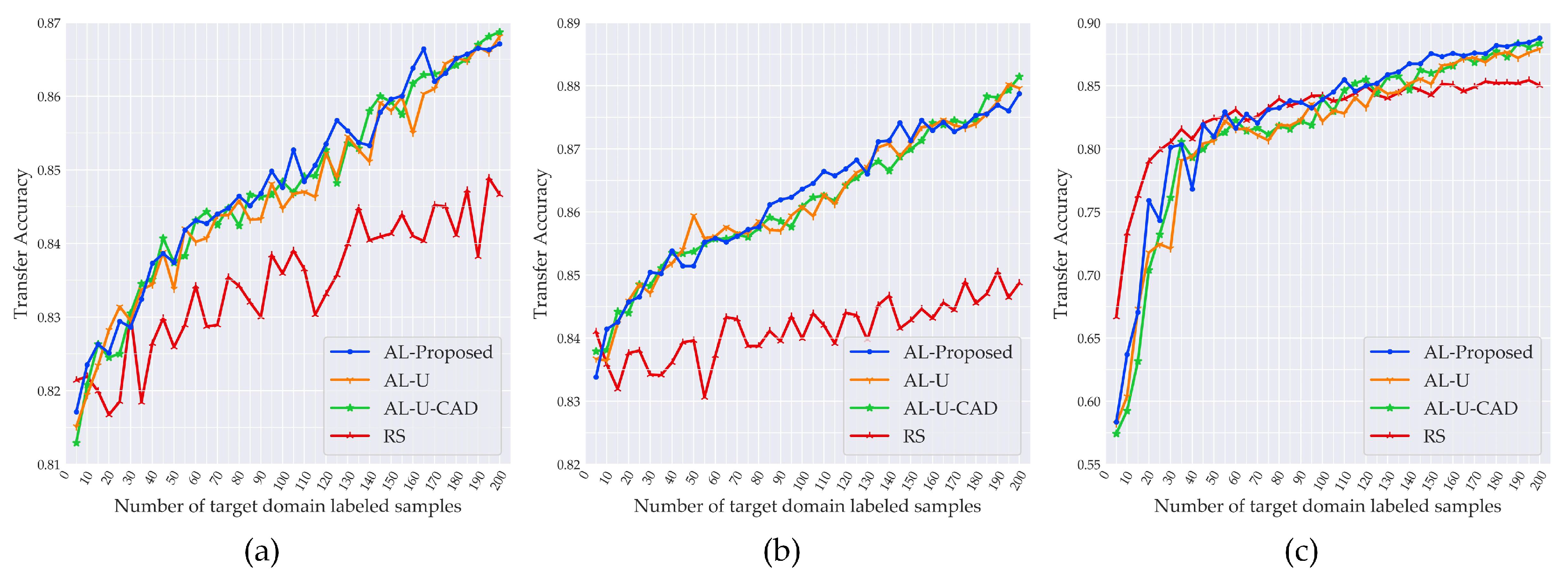
The experimental setup was as follows: based on the framework of the proposed method, the above sample selection strategies were used in the growing stage to update the training set, without changing the other processing steps of the framework, and their transfer accuracies were then compared. As described in Section 3.2, we used an incremental number sequence for , and each set of experiments was run 10 times, with the mean value used as the final result. The experimental results are shown in Figure 16.
In Figure 16a,b, the accuracies of the three active learning strategies were significantly better than that of RS, which demonstrated the effectiveness of active learning in improving the accuracy. However, as shown in Figure 16c, the accuracy of RS was significantly better than active learning when , and the accuracy of the active learning was only better than RS when . This unexpected phenomenon was also reported in some related studies, such as [24,32,33], and may be caused by the class imbalance problem when the number of samples is small. In the experiments, we constrained the procedure of RS to ensure that all the classes of ground objects were contained in the samples. Active learning paid greater attention to the samples with high uncertainty, and so when the number of samples was small and the uncertainty of certain classes was high, the acquired samples did not necessarily contain all the classes of samples, resulting in class imbalance. This problem is worthy of further study in follow-up research.
On the other hand, the accuracy achieved by RS proved the validity and reliability of the framework of the proposed method. In addition, from the above experimental results, the smaller the distribution difference between domains, the higher the accuracy improvement that active learning can bring compared to RS. The distribution difference was minimal in the second set of experiments; therefore, the accuracy improvement was the largest, while the accuracy improvement in the third set of experiments was the smallest as the distribution difference was the maximum.
For the results of the three active learning strategies, the AL-Proposed method outperformed the other two active learning strategies in most cases (particularly in the third set of experiments). The reason for this is that the AL-Proposed method could maintain the class balance of the target domain samples well through the diversity, and the measurement of diversity was irrelevant to the source domain samples. Therefore, when the distribution difference was greater, the advantage of the AL-Proposed method was more pronounced than that of the other two active learning strategies.
4. Conclusions
In this paper, we proposed a new active transfer learning method to address the problem of the low reusability of labeled samples in the applications of PolSAR images. Based on the deep forest network structure, the proposed method adjusts the training set and feature space simultaneously, and gradually improves the performance of the model in the target domain task. In this method, a new active learning strategy is used to ensure that every adjustment to the training set is the most helpful to improve the accuracy, and the augmented features are used to improve the transferability of knowledge between the source and target domain samples. At the same time, two filtering strategies are used to further improve the accuracy. The experimental results demonstrated that the proposed method was effective and reliable and able to perform well with different numbers of target domain labeled samples. The results also confirmed that the proposed method had good knowledge transfer capabilities in different groups of PolSAR images from different sensors and with various distribution differences.
In our future work, we will apply the proposed method in the specific applications of PolSAR images, such as the classification and change detection of multi-temporal images to evaluate its application potential in reducing labor costs and improving processing efficiency. In addition, as the proposed method is specific to PolSAR imagery, to apply it to other types of data, we could use a universal active learning strategy to acquire informative samples. However, the experimental results suggested that a targeted active learning strategy designed based on the specific tasks and data types tended to be more effective.
Author Contributions
Conceptualization: L.Z. and X.Q.; methodology: X.Q., K.S., and L.Z.; validation: X.Q. and K.S.; investigation: X.Q. and L.Z.; resources: J.Y. and P.L.; writing of original draft: X.Q. and L.Z.; writing review and editing: J.Y., X.Q., L.Z., and K.S.; supervision: J.Y. and P.L.; project administration: J.Y. and P.L.; funding acquisition: J.Y. All authors have read and agreed to the published version of the manuscript.
Funding
This research was funded by the National Natural Science Foundation of China (61971318, 41771377), the Hubei Provincial Natural Science Foundation of China (2019CFB484), and the Joint Fund of the Ministry of Education (6141A02022420).
Conflicts of Interest
The authors declare no conflict of interest.
References
- Pan, S.J.; Yang, Q. A Survey on Transfer Learning. IEEE Trans. Knowl. Data Eng. 2010, 22, 1345–1359. [Google Scholar] [CrossRef]
- Kamishima, T.; Hamasaki, M.; Akaho, S. TrBagg: A Simple Transfer Learning Method and its Application to Personalization in Collaborative Tagging. In Proceedings of the 2009 Ninth IEEE International Conference on Data Mining, Miami, FL, USA, 6–9 December 2009; pp. 219–228. [Google Scholar] [CrossRef] [Green Version]
- Lin, D.; An, X.; Zhang, J. Double-bootstrapping source data selection for instance-based transfer learning. Pattern Recognit. Lett. 2013, 34, 1279–1285. [Google Scholar] [CrossRef]
- Donahue, J.; Hoffman, J.; Rodner, E.; Saenko, K.; Darrell, T. Semi-supervised Domain Adaptation with Instance Constraints. In Proceedings of the 2013 IEEE Conference on Computer Vision and Pattern Recognition, Portland, OR, USA, 23–28 June 2013; pp. 668–675. [Google Scholar] [CrossRef] [Green Version]
- Liu, X.; Wang, G.; Cai, Z.; Zhang, H. Bagging based ensemble transfer learning. J. Ambient Intell. Humaniz. Comput. 2016, 7, 29–36. [Google Scholar] [CrossRef]
- Liu, B.; Xiao, Y.; Hao, Z. A Selective Multiple Instance Transfer Learning Method for Text Categorization Problems. Knowl. Based Syst. 2018, 141, 178–187. [Google Scholar] [CrossRef]
- Pereira, L.A.; da Silva Torres, R. Semi-supervised transfer subspace for domain adaptation. Pattern Recognit. 2018, 75, 235–249. [Google Scholar] [CrossRef]
- Zhang, L.; Guo, L.; Gao, H.; Dong, D.; Fu, G.; Hong, X. Instance-based ensemble deep transfer learning network: A new intelligent degradation recognition method and its application on ball screw. Mech. Syst. Signal Process. 2020, 140, 106681. [Google Scholar] [CrossRef]
- Pan, S.J.; Tsang, I.W.; Kwok, J.T.; Yang, Q. Domain Adaptation via Transfer Component Analysis. IEEE Trans. Neural Netw. 2011, 22, 199–210. [Google Scholar] [CrossRef] [Green Version]
- Duan, L.; Xu, D.; Tsang, I.W. Domain Adaptation From Multiple Sources: A Domain-Dependent Regularization Approach. IEEE Trans. Neural Netw. Learn. Syst. 2012, 23, 504–518. [Google Scholar] [CrossRef]
- Othman, E.; Bazi, Y.; Melgani, F.; Alhichri, H.; Alajlan, N.; Zuair, M. Domain Adaptation Network for Cross-Scene Classification. IEEE Trans. Geosci. Remote Sens. 2017, 55, 4441–4456. [Google Scholar] [CrossRef]
- Theckel Joy, T.; Rana, S.; Gupta, S.; Venkatesh, S. A Flexible Transfer Learning Framework for Bayesian optimization with Convergence Guarantee. Expert Syst. Appl. 2018, 115, 656–672. [Google Scholar] [CrossRef]
- Yan, K.; Kou, L.; Zhang, D. Learning Domain-Invariant Subspace Using Domain Features and Independence Maximization. IEEE Trans. Cybern. 2018, 48, 288–299. [Google Scholar] [CrossRef]
- Wang, Y.; Zhai, J.; Li, Y.; Chen, K.; Xue, H. Transfer learning with partial related “instance-feature” knowledge. Neurocomputing 2018, 310, 115–124. [Google Scholar] [CrossRef]
- Qin, X.; Yang, J.; Li, P.; Sun, W.; Liu, W. A Novel Relational-Based Transductive Transfer Learning Method for PolSAR Images via Time-Series Clustering. Remote Sens. 2019, 11, 1358. [Google Scholar] [CrossRef] [Green Version]
- Wang, Z.; Song, Y.; Zhang, C. Transferred Dimensionality Reduction. Machine Learning and Knowledge Discovery in Databases; Daelemans, W., Goethals, B., Morik, K., Eds.; Springer: Berlin/Heidelberg, Germany, 2008; pp. 550–565. [Google Scholar]
- Chang, H.; Han, J.; Zhong, C.; Snijders, A.M.; Mao, J. Unsupervised Transfer Learning via Multi-Scale Convolutional Sparse Coding for Biomedical Applications. IEEE Trans. Pattern Anal. Mach. Intell. 2018, 40, 1182–1194. [Google Scholar] [CrossRef] [PubMed] [Green Version]
- Siddhant, A.; Goyal, A.; Metallinou, A. Unsupervised Transfer Learning for Spoken Language Understanding in Intelligent Agents. arXiv 2018, arXiv:cs.CL/1811.05370. [Google Scholar] [CrossRef] [Green Version]
- Rochette, A.; Yaghoobzadeh, Y.; Hazen, T.J. Unsupervised Domain Adaptation of Contextual Embeddings for Low-Resource Duplicate Question Detection. arXiv 2019, arXiv:cs.CL/1911.02645. [Google Scholar]
- Passalis, N.; Tefas, A. Unsupervised Knowledge Transfer Using Similarity Embeddings. IEEE Trans. Neural Netw. Learn. Syst. 2019, 30, 946–950. [Google Scholar] [CrossRef]
- Liu, Y.; Ding, L.; Chen, C.; Liu, Y. Similarity-Based Unsupervised Deep Transfer Learning for Remote Sensing Image Retrieval. IEEE Trans. Geosc. Remote Sens. 2020, 1–18. [Google Scholar] [CrossRef]
- Deng, C.; Xue, Y.; Liu, X.; Li, C.; Tao, D. Active Transfer Learning Network: A Unified Deep Joint Spectral-Spatial Feature Learning Model for Hyperspectral Image Classification. IEEE Trans. Geosci. Remote Sens. 2019, 57, 1741–1754. [Google Scholar] [CrossRef] [Green Version]
- Wu, D. Active semi-supervised transfer learning (ASTL) for offline BCI calibration. In Proceedings of the 2017 IEEE International Conference on Systems, Man, and Cybernetics (SMC), Banff, AB, Canada, 5–8 October 2017; pp. 246–251. [Google Scholar] [CrossRef] [Green Version]
- Yan, Y.; Subramanian, R.; Lanz, O.; Sebe, N. Active transfer learning for multi-view head-pose classification. In Proceedings of the 21st International Conference on Pattern Recognition (ICPR2012), Tsukuba, Japan, 11–15 November 2012; pp. 1168–1171. [Google Scholar]
- Tang, X.; Du, B.; Huang, J.; Wang, Z.; Zhang, L. On combining active and transfer learning for medical data classification. IET Comput. Vis. 2019, 13, 194–205. [Google Scholar] [CrossRef]
- Wang, N.; Li, T.; Zhang, Z.; Cui, L. TLTL: An Active Transfer Learning Method for Internet of Things Applications. In Proceedings of the ICC 2019-2019 IEEE International Conference on Communications (ICC), Shanghai, China, 20–24 May 2019; pp. 1–6. [Google Scholar] [CrossRef]
- Zhou, Z.; Feng, J. Deep forest: Towards an alternative to deep neural networks. arXiv 2017, arXiv:1702.08835. [Google Scholar]
- Settles, B. Active Learning Literature Survey; University of Wisconsin-Madison: Madison, WI, USA, 2010; Volume 52. [Google Scholar]
- Schein, A.I.; Ungar, L.H. Active learning for logistic regression: An evaluation. Mach. Learn. 2007, 68, 235–265. [Google Scholar] [CrossRef]
- Demir, B.; Persello, C.; Bruzzone, L. Batch-Mode Active-Learning Methods for the Interactive Classification of Remote Sensing Images. IEEE Trans. Geosci. Remote Sens. 2011, 49, 1014–1031. [Google Scholar] [CrossRef] [Green Version]
- Brinker, K. Incorporating Diversity in Active Learning with Support Vector Machines. In Proceedings of the Twentieth International Conference (ICML 2003), Washington, DC, USA, 21–24 August 2003; pp. 59–66. [Google Scholar]
- Persello, C.; Bruzzone, L. Active Learning for Domain Adaptation in the Supervised Classification of Remote Sensing Images. IEEE Trans. Geosci. Remote Sens. 2012, 50, 4468–4483. [Google Scholar] [CrossRef]
- Yang, J.; Li, S.; Xu, W. Active Learning for Visual Image Classification Method Based on Transfer Learning. IEEE Access 2018, 6, 187–198. [Google Scholar] [CrossRef]
- Cloude, S.R.; Pottier, E. An entropy based classification scheme for land applications of polarimetric SAR. IEEE Trans. Geosci. Remote Sens. 1997, 35, 68–78. [Google Scholar] [CrossRef]
- Deng, W.; Lendasse, A.; Ong, Y.; Tsang, I.W.; Chen, L.; Zheng, Q. Domain Adaption via Feature Selection on Explicit Feature Map. IEEE Trans. Neural Netw. Learn. Syst. 2019, 30, 1180–1190. [Google Scholar] [CrossRef]
- Fernando, B.; Habrard, A.; Sebban, M.; Tuytelaars, T. Unsupervised Visual Domain Adaptation Using Subspace Alignment. In Proceedings of the 2013 IEEE International Conference on Computer Vision, Sydney, Australia, 1–8 December 2013; pp. 2960–2967. [Google Scholar] [CrossRef] [Green Version]
- Borgwardt, K.M.; Gretton, A.; Rasch, M.J.; Kriegel, H.P.; Schölkopf, B.; Smola, A.J. Integrating Structured Biological Data by Kernel Maximum Mean Discrepancy. Bioinformatics 2006, 22, 49–57. [Google Scholar] [CrossRef] [Green Version]
Figure 1.
The process of active learning.

Figure 2.
Flowchart of multi-grain scanning for sequence data.

Figure 3.
Structure of a cascade forest.

Figure 4.
Structure of the proposed method.

Figure 5.
Diagram of a single cascade layer. A cascade layer consists of two completely random tree forests and two random forests.
Figure 5.
Diagram of a single cascade layer. A cascade layer consists of two completely random tree forests and two random forests.

Figure 6.
Flowchart of the proposed active learning strategy.

Figure 7.
Flowchart of the filtering stage.

Figure 8.
Three polarimetric synthetic aperture radar (PolSAR) images of Wuhan. (a) Pauli RGB image of RD-2 on 7 December 2011. (b) Pauli RGB image of RADARSAT-2 (RD-2) on 6 July 2016. (c) Pauli RGB image of Gaofen-3 (GF-3) on 29 May 2017. (d) Ground truth map of RD-2 on 7 December 2011. (e) Ground truth map of RD-2 on 6 July 2016. (f) Ground truth map of GF-3 on 29 May 2017.

Figure 9.
Two polarimetric synthetic aperture radar (PolSAR) images of Suzhou. (a) Pauli RGB image of RD-2 on 12 August 2008. (b) Pauli RGB image of RD-2 on 9 March 2016. (c) Ground truth map of RD-2 on 12 August 2008. (d) Ground truth map of RD-2 on 9 March 2016.
Figure 9.
Two polarimetric synthetic aperture radar (PolSAR) images of Suzhou. (a) Pauli RGB image of RD-2 on 12 August 2008. (b) Pauli RGB image of RD-2 on 9 March 2016. (c) Ground truth map of RD-2 on 12 August 2008. (d) Ground truth map of RD-2 on 9 March 2016.

Figure 10.
Distributions of the first group of experimental data in the H-Alpha plane. (a) The distribution of the 1000 source domain samples. (b) The distribution of the 1000 target domain samples.
Figure 10.
Distributions of the first group of experimental data in the H-Alpha plane. (a) The distribution of the 1000 source domain samples. (b) The distribution of the 1000 target domain samples.

Figure 11.
Distributions of the second group of experimental data in the H-Alpha plane. (a) The distribution of the 1000 source domain samples. (b) The distribution of the 1000 target domain samples.
Figure 11.
Distributions of the second group of experimental data in the H-Alpha plane. (a) The distribution of the 1000 source domain samples. (b) The distribution of the 1000 target domain samples.

Figure 12.
Distributions of the third group of experimental data in the H-Alpha plane. (a) The distribution of the 1000 source domain samples. (b) The distribution of the 1000 target domain samples.
Figure 12.
Distributions of the third group of experimental data in the H-Alpha plane. (a) The distribution of the 1000 source domain samples. (b) The distribution of the 1000 target domain samples.

Figure 13.
The mean and standard deviation of the transfer accuracies of the first set of experiments.
Figure 13.
The mean and standard deviation of the transfer accuracies of the first set of experiments.

Figure 14.
The mean and standard deviation of the transfer accuracies of the second set of experiments.
Figure 14.
The mean and standard deviation of the transfer accuracies of the second set of experiments.

Figure 15.
The mean and standard deviation of the transfer accuracies of the third set of experiments.
Figure 15.
The mean and standard deviation of the transfer accuracies of the third set of experiments.

Figure 16.
Comparison of the effect of different sample selection strategies. (a–c) are the results of the three sets of experimental data. The proposed active learning strategy (AL-Proposed), active learning using only uncertainty (AL-U), active learning using uncertainty and the cosine angle distance (AL-U-CAD), and random sampling (RS).


Table 1.
Transfer accuracies (%) of different methods in the three sets of experiments.
| Data Set | Number of | Baseline | BETL | TrBagg | SMIDA | SSTCA | Proposed |
|---|---|---|---|---|---|---|---|
| 5 | 80.50 | 73.57 ± 5.02 | 74.72 ± 7.56 | 79.42 ± 0.47 | 74.18 ± 5.29 | 81.70 ± 0.58 | |
| Wuhan 2011 | 50 | 80.50 | 73.32 ± 5.29 | 81.69 ± 1.07 | 80.90 ± 0.96 | 79.18 ± 1.92 | 83.74 ± 0.42 |
| to | 100 | 80.50 | 78.90 ± 2.31 | 81.53 ± 0.78 | 81.47 ± 0.73 | 78.52 ± 1.47 | 84.76 ± 0.45 |
| Wuhan 2017 | 150 | 80.50 | 79.20 ± 1.86 | 82.17 ± 1.05 | 82.63 ± 0.52 | 78.26 ± 1.66 | 85.96 ± 0.67 |
| 200 | 80.50 | 80.61 ± 1.94 | 83.19 ± 0.66 | 81.90 ± 2.62 | 79.59 ± 2.13 | 86.71 ± 0.21 | |
| 5 | 81.90 | 72.02 ± 5.88 | 63.57 ± 22.17 | 79.49 ± 0.90 | 76.91 ± 1.18 | 83.38 ± 0.45 | |
| Wuhan 2016 | 50 | 81.90 | 74.59 ± 6.72 | 81.30 ± 0.81 | 81.63 ± 0.91 | 80.53 ± 0.59 | 85.14 ± 0.29 |
| to | 100 | 81.90 | 78.30 ± 3.00 | 82.20 ± 1.58 | 82.18 ± 0.95 | 81.94 ± 0.78 | 86.36 ± 0.28 |
| Wuhan 2017 | 150 | 81.90 | 81.14 ± 1.94 | 82.44 ± 0.75 | 83.01 ± 1.06 | 82.35 ± 0.90 | 87.13 ± 0.27 |
| 200 | 81.90 | 81.10 ± 2.12 | 83.34 ± 0.69 | 83.42 ± 0.79 | 82.45 ± 1.04 | 87.87 ± 0.32 | |
| 5 | 58.40 | 51.94 ± 4.02 | 46.18 ± 14.92 | 77.02 ± 1.22 | 59.83 ± 5.41 | 58.34 ± 6.78 | |
| Suzhou 2008 | 50 | 58.40 | 65.73 ± 9.07 | 70.98 ± 9.72 | 80.20 ± 1.12 | 77.60 ± 2.97 | 80.95 ± 2.24 |
| to | 100 | 58.40 | 69.45 ± 8.80 | 77.11 ± 5.50 | 81.84 ± 1.09 | 82.26 ± 1.01 | 83.91 ± 1.25 |
| Suzhou 2016 | 150 | 58.40 | 73.53 ± 7.88 | 76.40 ± 4.22 | 82.14 ± 0.73 | 82.12 ± 1.26 | 86.73 ± 0.70 |
| 200 | 58.40 | 79.51 ± 3.00 | 80.57 ± 3.11 | 83.55 ± 0.96 | 81.30 ± 2.83 | 88.76 ± 0.41 | |
| Average computational time (s) | 3.6 | 19.6 | 4.1 | 9.3 | 23.5 | 130 | |
Table 2.
The variation of the maximum mean discrepancy (MMD) and divergence between domains (DBD) during the growing stage.
Table 2.
The variation of the maximum mean discrepancy (MMD) and divergence between domains (DBD) during the growing stage.
| Data Number | MMD | DBD | ||
|---|---|---|---|---|
| Before | After | Before | After | |
| 1 | 1.9101 | 1.5093 | 97.91% | 97.57% |
| 2 | 0.9459 | 0.7086 | 95.83% | 94.55% |
| 3 | 1.2600 | 0.9229 | 98.22% | 97.24% |
Table 3.
Performance of the proposed method under different values of W and N.
| Parameters | Parameter Setting | Wuhan 2011 to Wuhan 2017 | Wuhan 2016 to Wuhan 2017 | Suzhou 2008 to Suzhou 2016 | Average Computational Time (s) |
|---|---|---|---|---|---|
| W | 86.27 ± 0.92 | 87.30 ± 0.62 | 87.04 ± 0.68 | 128.3 | |
| 86.34 ± 0.49 | 87.85 ± 0.61 | 87.63 ± 0.60 | 173.5 | ||
| 86.71 ± 0.21 | 87.87 ± 0.32 | 88.76 ± 0.41 | 190.1 | ||
| 87.39 ± 0.16 | 87.80 ± 0.43 | 88.43 ± 0.38 | 257.0 | ||
| N | 86.77 ± 0.38 | 87.62 ± 0.63 | 88.67 ± 0.40 | 529.2 | |
| 86.71 ± 0.21 | 87.87 ± 0.32 | 88.76 ± 0.41 | 190.1 | ||
| 86.76 ± 0.56 | 87.98 ± 0.53 | 87.96 ± 0.33 | 136.9 | ||
| 86.87 ± 0.41 | 87.82 ± 0.24 | 87.95 ± 0.52 | 113.7 |
© 2020 by the authors. Licensee MDPI, Basel, Switzerland. This article is an open access article distributed under the terms and conditions of the Creative Commons Attribution (CC BY) license (http://creativecommons.org/licenses/by/4.0/).
Share and Cite
MDPI and ACS Style
Qin, X.; Yang, J.; Zhao, L.; Li, P.; Sun, K. A Novel Deep Forest-Based Active Transfer Learning Method for PolSAR Images. Remote Sens. 2020, 12, 2755. https://0-doi-org.brum.beds.ac.uk/10.3390/rs12172755
AMA Style
Qin X, Yang J, Zhao L, Li P, Sun K. A Novel Deep Forest-Based Active Transfer Learning Method for PolSAR Images. Remote Sensing. 2020; 12(17):2755. https://0-doi-org.brum.beds.ac.uk/10.3390/rs12172755
Chicago/Turabian StyleQin, Xingli, Jie Yang, Lingli Zhao, Pingxiang Li, and Kaimin Sun. 2020. "A Novel Deep Forest-Based Active Transfer Learning Method for PolSAR Images" Remote Sensing 12, no. 17: 2755. https://0-doi-org.brum.beds.ac.uk/10.3390/rs12172755
Note that from the first issue of 2016, this journal uses article numbers instead of page numbers. See further details here.