Multi-Hazard Exposure Mapping Using Machine Learning for the State of Salzburg, Austria
by
 , , and
Thimmaiah Gudiyangada Nachappa
1 ,
,
Omid Ghorbanzadeh
1,* ,
,
Khalil Gholamnia
2 and
and
Thomas Blaschke
1
1
Department of Geoinformatics–Z_GIS, University of Salzburg, 5020 Salzburg, Austria
2
Department of Remote Sensing and GIS, University of Tabriz, Tabriz 5166616471, Iran
*
Author to whom correspondence should be addressed.
Remote Sens. 2020, 12(17), 2757; https://0-doi-org.brum.beds.ac.uk/10.3390/rs12172757
Submission received: 10 August 2020
/
Revised: 21 August 2020
/
Accepted: 24 August 2020
/
Published: 25 August 2020
(This article belongs to the Special Issue GeoAI: Integration of Artificial Intelligence, Machine Learning and Deep Learning with Remote Sensing)
Abstract
:We live in a sphere that has unpredictable and multifaceted landscapes that make the risk arising from several incidences that are omnipresent. Floods and landslides are widespread and recurring hazards occurring at an alarming rate in recent years. The importance of this study is to produce multi-hazard exposure maps for flooding and landslides for the federal State of Salzburg, Austria, using the selected machine learning (ML) approach of support vector machine (SVM) and random forest (RF). Multi-hazard exposure maps were established on thirteen influencing factors for flood and landslides such as elevation, slope, aspect, topographic wetness index (TWI), stream power index (SPI), normalized difference vegetation index (NDVI), geology, lithology, rainfall, land cover, distance to roads, distance to faults, and distance to drainage. We classified the inventory data for flood and landslide into training and validation with the widely used splitting ratio, where 70% of the locations are used for training, and 30% are used for validation. The accuracy assessment of the exposure maps was derived through ROC (receiver operating curve) and R-Index (relative density). RF yielded better results for both flood and landslide exposure with 0.87 for flood and 0.90 for landslides compared to 0.87 for flood and 0.89 for landslides using SVM. However, the multi-hazard exposure map for the State of Salzburg derived through RF and SVM provides the planners and managers to plan better for risk regions affected by both floods and landslides.
1. Introduction
Natural disasters have a stern influence the local community and can take numerous years to recuperate from the consequences [1]. Natural disasters that affect the human inhabitants have been arising at a frightening regularity across the world in recent years. The principal source of the catastrophe hangs on the exposure of the area to the hazard. Natural hazards are significant hostile events escalating from the natural as well as anthropological processes that influence the occurrences of flooding, landslides, earthquakes, wildfires, volcanoes, and tsunamis [2]. Natural hazards are often measured in separation, though there is a more significant cause to assess hazards holistically that helps in managing the intricate threats located in any region. "Multi-hazard" is a term coined by the United Nations within the context of UN sustainable goals along with the agenda 21 promoting risk reduction and disaster management as part of the sustainability program [3]. Multi-hazard assessments have increased in the past couple of years, where several natural hazards have impacted a region. Multi-hazards can cause more severe damages than a single hazard affecting transportation, damages to infrastructures, degradation of environmental conditions, and threaten human lives [4].
Flooding is considered one of the dangerous natural hazards that is happening quite regularly in recent times throughout the world. Floods are natural occurrences that arise following an extended period of rainfall or snowmelt in amalgamation with adverse circumstances [5]. Worldwide, the incidence of flooding has intensified by 40% over the previous two decades [6]. The increase in floods regularly is owing to the surge in ecological degradation such as rapid urbanization, the surge in population growth, and speedy deforestation [7]. Some physiographical factors greatly influence floodings like topography, geomorphology, and climate change [8,9]. Floods become a disaster once it impacts human lives, infrastructure, and settlements causing probable indemnities. If the flooding occurs at a regular interval, then the damages are also on the higher side impacting severely on the life of living beings, impacting the economy, disrupting the transportation networks, destabilizing the ecological equilibrium, and damages to the infrastructures [10]. The amount of individuals existing in the flood hazard region is projected to be about 1.3 billion by the end of 2050 [11]. Assessment of flood is quite significant for socioeconomic and ecological consequences [12].
Landslides are described as the gravitational movement of the mass of rocks or debris down a slope [13]. In a broad-spectrum landslide are mass movements, which contain rock falls, mudslides, and debris flows. The categorization of landslides is generally based on the type of material like rock, debris, earth, or mud; and the movement type, such as fall, topple, avalanche, slide, flow, or spread. Landslides are triggered by various natural processes like substantial and protracted rainfall, earthquakes, snowmelt or human-made processes like road constructions, infrastructures, deforestations, or even the combination of natural and human-made processes [14]. Landslides are occurrences of land degradation that alter the topographies of the site, instigating soil erosion, habitat destruction, environmental complications, and structural damages [15]. Landslides are happening at an alarming rate in recent times owing to the development and rapid urbanization without proper planning and studies on the region resulting in frequent landslides [16]. Owing to the frequent landslides, there has been substantial consideration from the scientific community and policymakers in understanding the landslides are the assessment of landslides [17]. Landslides, in general, are measured as natural occurrences. However, mostly they are frequently initiated by the influence of anthropological activities [18].
Most parts of the world have varying and compound landscapes where the risk from a numerous event are ubiquitous. Exposure analysis of any natural hazard is an important task to forecast the imminent incidences of natural hazards. Flood exposure is vital for management strategies on the prevention and mitigation of floods [19]. To understand and study the impact of landslides on human and economic losses, it is important to comprehend a region’s exposure to landslides. Landslide exposure is the potential impact of a particular type of landslide on a specific area in the future [1]. Landslide exposure is the spatially explicit quantification of the probability of the occurrence of landslides in the future based on the effects of influencing factors in the given area [20].
Natural hazard assessments have been analyzed utilizing diverse models like frequency ratio (FR) [21,22], analytical hierarchicalp [23,24], analytical network process [25], support vector machines [26,27], random forest [28], evidence belief function [29], fuzzy logic and ensembles [30,31], Dempster–Shafer [32,33], K-nearest neighbor [9], decision tree [34,35], logistic regression [36,37], artificial neural networks [38], and deep learning algorithms of the recurrent neural network (RNN) and convolutional neural network (CNN) [39]. Lately, machine learning (ML) approaches have been widely used for natural hazard evaluations corresponding to landslides, floods, and wildfires [2,40,41,42,43,44]. All the methodologies have their particular qualities and drawbacks, and each model’s performance varies based on the input data used, the structure of the model, and the accuracy of the model. However, there is no indication that a specific model must be used for a specific situation, hazard, or study area [45]. In the latest studies, ML methods like naïve Bayes along with naïve Bayes tree was equated with multi-criteria decision analysis technique like "Vise Kriterijumska Optimizacija I Kompromisno Resenje" (VIKOR), "Technique for Order Preference by Similarity to an Ideal Solution" (TOPSIS), and simple average weight (SAW) that resulted in ML model yielding superior prediction equated to Multi Criteria Decision Analysis (MCDA) [8].
Similarly, evidence belief function and ensemble methods were used for flood susceptibility and equated with TOPSIS, classification and regression trees (CART), and VIKOR and frequency ratio (FR) techniques where evidence belief function model yielded greater precision [46,47,48]. Furthermore, superior ML approaches as simulate annealing (feature selection) using the resampling algorithm were used for deriving the susceptibility maps for floods [49]. Already diverse ML methods and deep learning approaches have been used in landslide detection studies [50]. Recurrent neural network (RNN) and multilayer perceptron neural network (MLP-NN) techniques characteristically entail an input data set from orthophotos or LiDAR-derived datasets. This also relates to the use of textural features for landslide detection [51].
Austria is an alpine country enclosed by land and situated in Europe with an approximate area around 84,000 km2 having 8.7 million population [52]. Owing to the setting of the country in the alpine range and having climatic environment, natural hazards like landslides, avalanches, and floods pose a significant risk to the low-lying areas within the country. More than 1 million habitants residing and 13% of the structures are situated in flood-prone regions of Austria [53]. In 2002, 2005, 2006, and 2013, large scale flooding occurred along the Danube and its tributaries in Austria [54]. The State of Salzburg is one of the nine federal states in Austria, and Salzburg is the capital of the state of Salzburg. The region has been impacted by severe flooding and landslides in recent times, and the region is very dynamic concerning its economic and growths [55].
In this research, we chose SVM and RF as a machine learning algorithm for multi-hazard exposure mapping for the state of Salzburg in Austria. A multi-hazard exposure map is a basis for multi-hazard risk assessment and the main focus of this research. There has been no study yet been done on multi-hazard exposure mapping for the state of Salzburg which is impacted frequently by landslides and floods, and this could be helpful for planners and policymakers to consider regions impacted by multi-hazard and manage mitigating measures.
2. Study Area
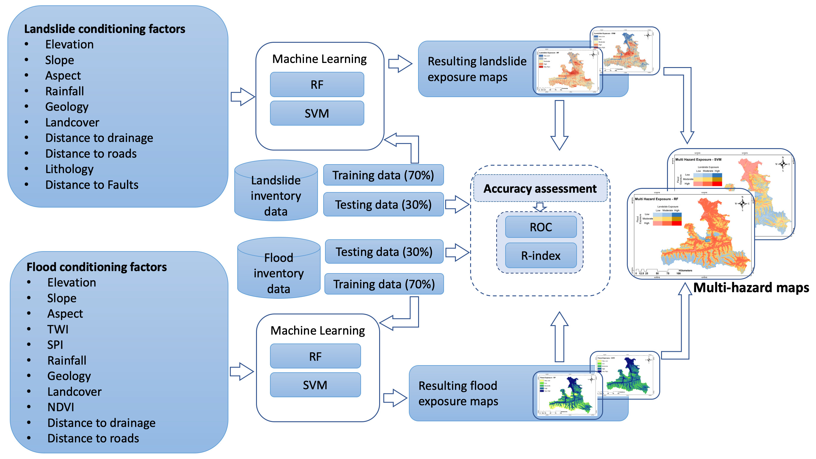
The State of Salzburg in Austria, as seen in the Figure 1, is one of the nine federal states of Austria. The State of Salzburg covers an area of 7156.03 km2 and has a population of 531,000 with a density of 74/km2. Salzach is a primary river which runs through the alps and has a drainage basin of 6829 km2. This also includes sizable parts of the northern limestone and central-eastern alps. Salzach is the main river which lies about 83% in Austria and the rest in southern Germany. The Großvenediger is the highest peak that has an altitude of 3657 meters above sea level. The State of Salzburg is enclosed by roughly 370,000 hectares of forest, conforming to 52% of its entire area. The forests have great economic significance and are vital for the protection against natural hazards.
Landslides and floods are a prevalent natural hazard in the study area. Landslide incident in the region is determined by numerous aspects, specifically lithology, tectonic structure, geomorphology (mainly slope, angle, and aspect), and land use. The geomorphological situation of Austria significantly contributes to the likelihood of landslide happening, as the Alps constitute 62% of the region. Torrents and avalanches jeopardize around 75% of the communities in Austria [56]. The degradation of permafrost in the alps owing to the surge in temperatures can lead to slope volatilities and threatens settlements and transportations systems. In Austria, several human-made infrastructures, such as roads and buildings, are highly vulnerable to landslides caused by heavy rainstorms and long-lasting rain events. During the years 2002, 2005, 2006, and 2013, the Salzach basin experienced huge flooding [54]. The upsurge of annual daily precipitation in several regions signifies the escalation in the prospect of severe flooding in the alpine regions [57,58]. The state of Salzburg is very dynamic regarding its economy and growths and attracts a lot of tourists [55].
3. Data & Methodology
3.1. Inventory Data
The inventory data plays a significant role in the assessment of exposure maps of any natural hazards. Consequently, it is imperious to have a good set of inventory for the analysis.
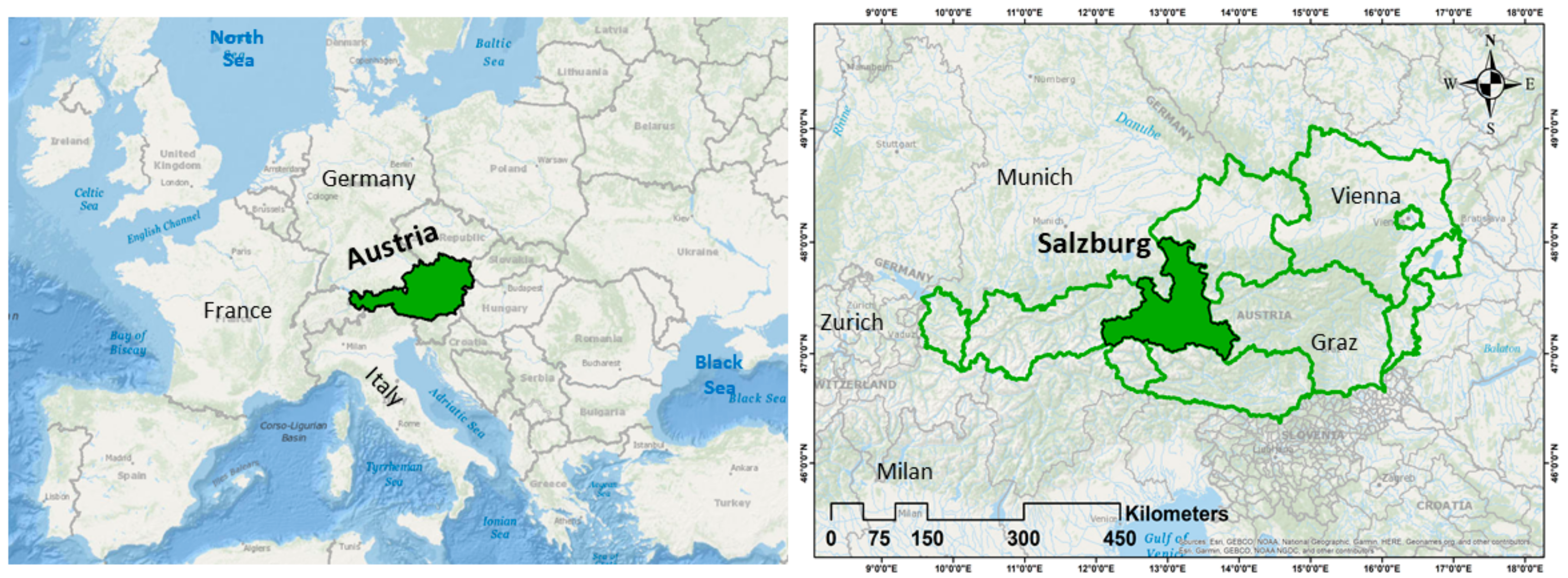
The landslide inventory for this study was attained from the Geological Survey of Austria (GBA), who provided the point inventory of landslides mainly of rockfalls/rockslides (25%), complex movements (6%), and landslides (69%). Further information can be found at GBA (www.geologie.ac.at). There have been quite a significant number of landslides happening in Austria, and only a limited number of landslide locations are provided in the inventory data. The provided inventory data has limitations regarding completeness and up-to-datedness. To derive the accuracy of the model through model validation, the landslide inventory is required that is not used for training the model. Hence it is essential to allocate the dataset into two portions. The first part is applied to train the models and is called the training dataset, and the second part is used for validating the model’s performance and is referred to as the validation dataset. To forecast the incidences of potential flooding, it is fundamental to evaluate the incidence of historic flooding as the historical incident data has a solid relationship with the future occurrences of flooding [59]. The flood inventory was built centred on the Hochwasserrisikozonierung—Flood risk zoning (HORA—https://www.hora.gv.at/) with HQ30 for Austria. The flood HQ30 having polygon coverage and randomized locations was used for deriving flood locations for each polygon within the HQ30 flood data. There are no typical approaches for the selection of training and validation samples [1]; the most shared ratio for training and validation samples is 70/30 [60]. This method has been used for various natural hazard studies [61]. The landslide and flood inventory dataset were divided randomly into two groups, with 70% used for training and 30% used for validating the results. Figure 2 shows the flood and landslide inventory data categorized into training and testing data.
3.2. Influencing Factors
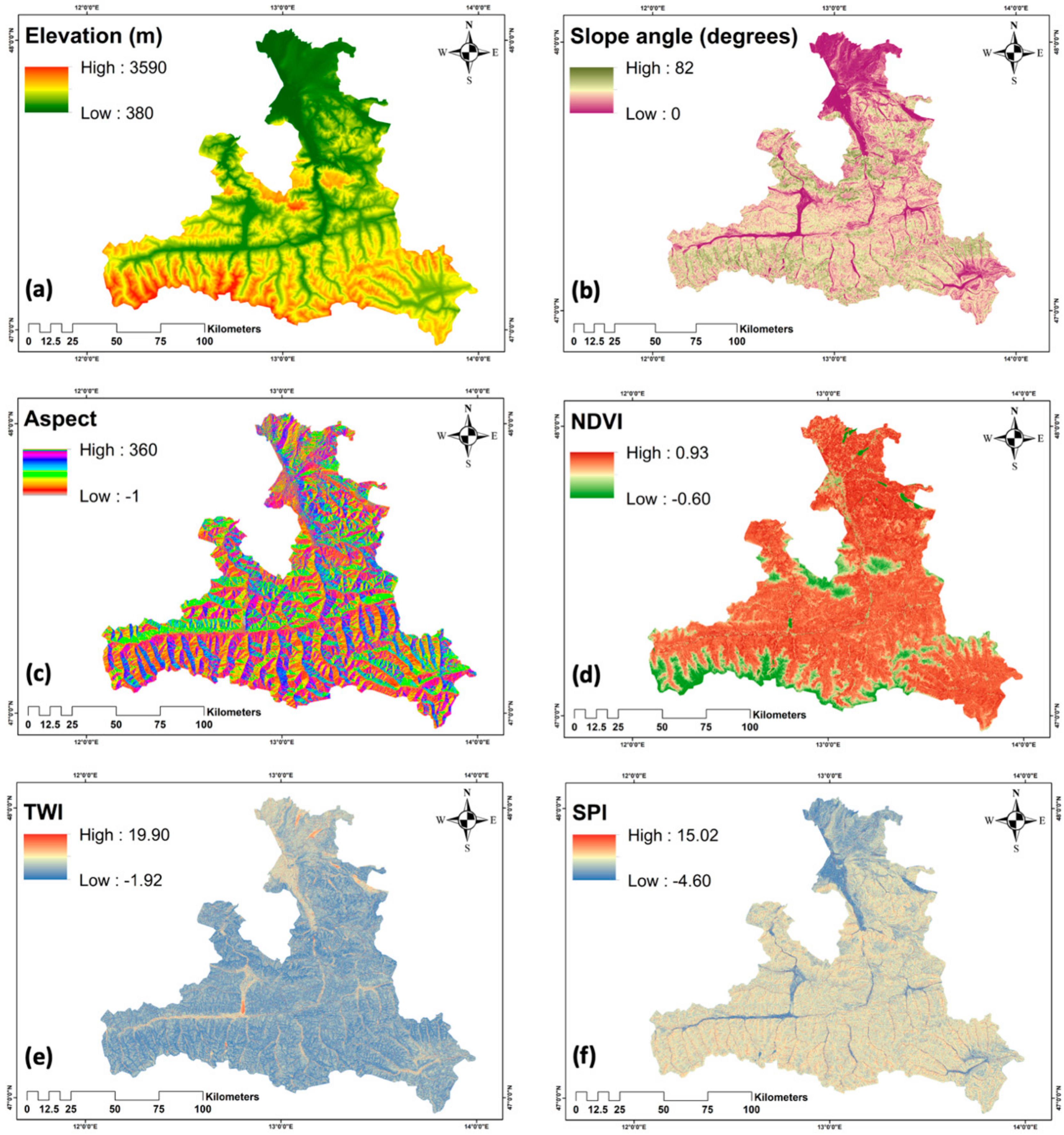
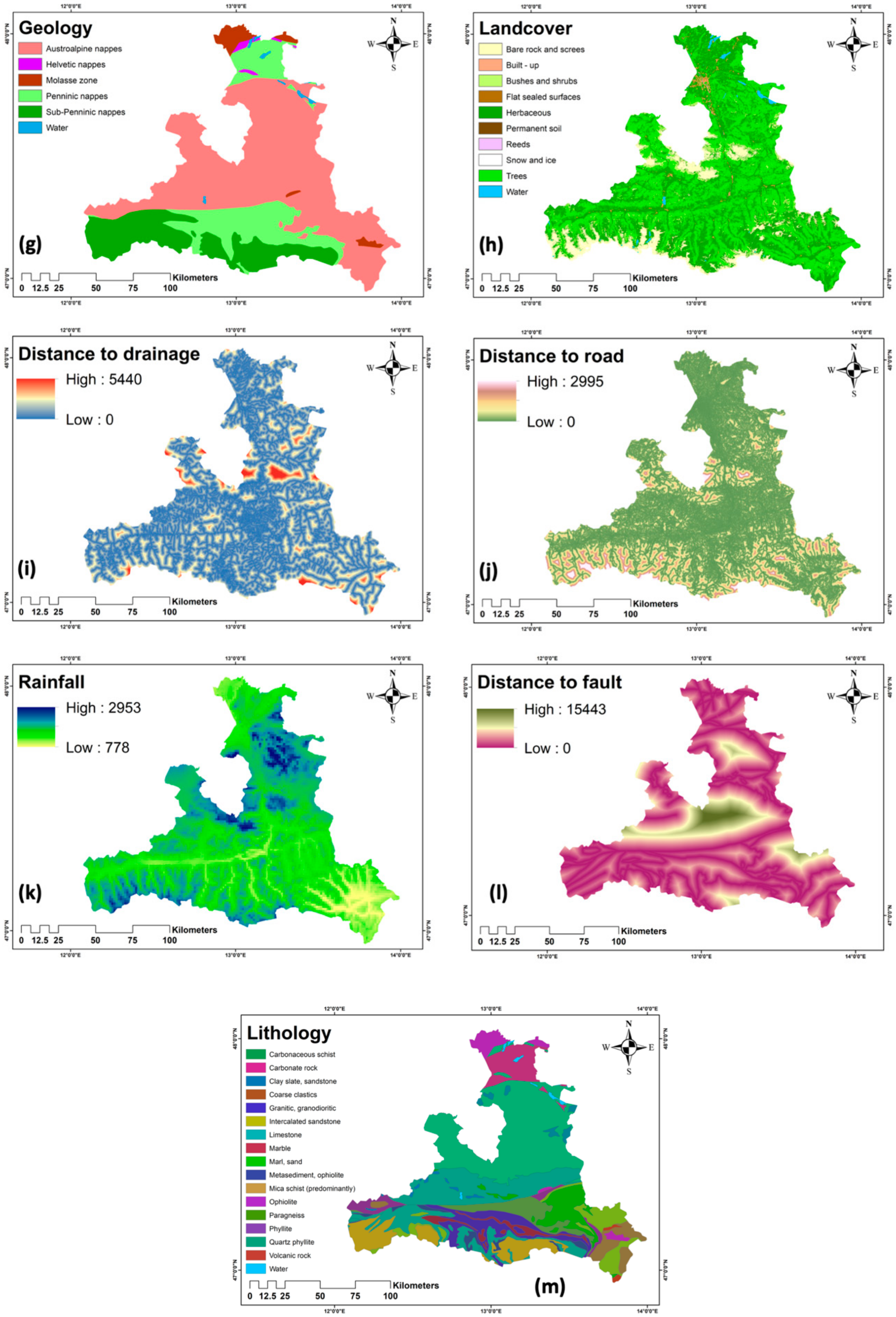
It is pivotal to control the influencing factors for various natural hazards for the purpose of exposure mapping [21]. There are no predefined benchmarks for selecting the influencing factors for exposure mapping. Ideally, the selected influencing factors should be operative, quantifiable, and non-uniform. Established on the geomorphological characteristics, literature, data availability, and expert feedback, a total of thirteen influencing factors were chosen for this study area for flooding and landslides. For landslide exposure mapping, ten influencing factors were selected, i.e., elevation, slope angle, slope aspect, distance to roads, distance to drainage, rainfall, land use, faults, geology, and lithology. For flood exposure mapping, eleven influencing factors such as elevation, slope, aspect, topographic wetness index (TWI), stream power index (SPI), distance to drainage, geology, distance to roads, rainfall, NDVI, and land cover. Figure 3 shows the influencing factors for both flood and landslide for multi-hazard exposure mapping.
A freely accessible digital elevation model (DEM) with 10 m spatial resolution for the State of Salzburg, downloadable through the Open Data Portal Austria (www.data.gv.at) was used for deriving the auxiliary data like slope, aspect, and hydrological aspects such as TWI and SPI. Geology, lithology, faults, and drainage data were obtained from the Geological Survey of Austria (GBA). Rainfall information data for Austria was obtained from the ÖKS15—Klimaszenarien für Österreich from the center of the Climate Change Centre Austria (CCCA) data center for the State of Salzburg. Normalized Difference Vegetation Index (NDVI) was transferred from land viewer EOS, and the Land Information System Austria (LISA) was used for attaining the land cover data. The road networks were downloaded from the humanitarian open street map network (HOTOSM). Table 1 shows the influencing factors for flood and landslides for this study, and Figure 2 shows the influencing factor used for the study area.
There is no traditional or acknowledged standard for the classification of conditioning factors [62]. The study area and the relevance of each factor for the study area were taken into considerations when conditioning factors were classified along with the information available within the dataset.
Elevation plays an important influence on flood and landslide exposure mapping [23]. The elevation describes the deepest and the maximum range point in the region. The elevation influences the geomorphological and geological processes [63]. It can affect the topographic attributes that lead to spatial variability of different landscape processes, and it can influence the vegetation distribution. As the elevation ascents in the Alpine region, vegetation fluctuates are witnessed.
The slope is decisive in flooding as this controls the velocity of the surface runoff and upright filtration that impacts the flood exposure. The slope is quantified as the exterior guide for flood exposure [64]. The slope is considered as the key influencing factor straightforwardly connected to landslide exposure analysis as this influences the failure of slope [65]. Landscapes that have sharper slopes are generally more susceptible to failure. Aspect is an important influence for both flood and landslide exposure analysis as this defines the direction of the slope.
Land cover describes the variation in exceedingly separated areas within the region and provides insights on the activity [66]. Land cover is a key influencing factor for flood and landslide evaluations [67]. Land cover is categorized as; Built-up, Flat sealed surfaces, Permanent soil, Bare Rock and Screes, Water, Snow and Ice, Trees, Bushes and Shrubs, Herbaceous, and Reeds.
Rainfall is an essential and crucial activating aspect for both flooding and landslides [68]. Rainfall characters differ by climate circumstances and topographical characters, and this can instigate substantial time-based and spatial variances in the rainfall occurrence. The rainfall is measured in mm.
Geology of the region exhibits a substantial role in flood and landslide exposure due to the understanding of lithological elements [69]. Regions that have greater porous soil and rigid endurance rocks manage to have stumpy channel densities [7]. There are six geological units in our study region, mainly Helvetic nappes, Austroalpine nappes, Penninic nappes, Molasse zone, Sub-Penninic nappes, and water.
Roads are considered as the critical anthropogenic factor that influences the flooding and occurrences of landslides [39,70].
Distance to drainage is a key influencing factor in flood exposure as this influences the extent of the flooding, magnitude and delivers water that triggers material saturation resulting in landslides [2,71].
Lithology is largely acknowledged as the important influencing factors in landslide exposure studies [69]. Lithological components differ in terms of geological strength indices, exposure to failure, and permeability [72]. Typically, the mass movements slide along a rock stratum with low strength and poor permeability. We have seventeen lithological units in our study area.
Distance to fault determines the incidence of landslides as faults build a break amid two distinguishing lithological units and create fractures and joints within the lithological unit that can propagate landslide activity. Geological faults are accountable for activating a huge amount of landslides because the tectonic breaks usually decrease the surrounding rock strength.
The topographic wetness index (TWI) is the gathering of water flow at any condition owing to the flow trends towards downstream owing to the gravitation in the catchment [73]. The TWI is calculated using the Equation (1) [74,75] given below where defined as the aggregate of the upslope part that is being consumed through a point and is the angle of slope at that particular point in degrees.
The stream power index (SPI) is the degree of the erosive supremacy of flowing water. The SPI is estimated based on the slope and the specific area using the Equation (2) [74] as given below where the is the particular zone of the catchment measured in m2/m of the particular catchment, and is the angle of the given slope angle at that particular point measured in degrees.
The normalized difference vegetation index (NDVI) processes the vegetation of a region based on how the vegetation reflects the light for particular frequencies (absorbing and reflection). This is quite decisive for flooding and landslides. This index defines values from −1 to +1 and calculated using the Equation (3) [76] given below where the NIR is the reflectance in the near-infrared spectrum and RED is the reflection in the red range of the spectrum.
3.3. Methodology
Machine learning (ML) approaches have recently been extensively used and contributed towards the evolution of prediction systems offering enhanced and enriched performance and efficient solutions [77]. ML methodologies have continually advanced and established their suitability for natural hazard assessments having better accuracy compared to the traditional approaches. Various ML approaches have been used for exposure mapping of natural hazards like floods, landslides, and wildfires [42,78,79]. However, there is no considerable evidence that a specific ML approach is best suited for a specific hazard assessment as this completely depends greatly on the inventory data and the influencing factors selected for the study area. ML is independent of any domain expert knowledge like the multi-criteria decision analysis approaches. For the multi-hazard exposure study, we have selected RF and SVM as two ML approaches for deriving the exposure maps for flood and landslide exposure.
3.3.1. Support Vector Machine (SVM)
SVM is a machine learning approach based on data mining and one of the influential supervised algorithms used for classification and regression. SVM was established on the basis of statistical learning theory where the input data is transformed into a new feature space, and a decision function is established in the new feature space through the optimal hyperplane. SVM is generally used along with a defined group of liner indicator equations for the functional valuations [80]. SVM provides superior performance and higher outputs, even with inadequate input data points is also acknowledged as the maximum-margin process [66]. SVM maps the data points into an elevated dimensional feature space using non-linear transformers while creating the best hyperplane, and this is based on statistical learning [81]. The finest hyperplane is achieved while unravelling precincts amongst the described classification of the problematic are highest. SVM’s have two layers and are unidirectional, which can implement various activation kernel functions such as linear, polynomial, radial, or sigmoid that influences the performance of the model [82,83]. As for the kernels, four kernel categories were used in this methodology to comprehend the effectiveness of categorization and the type as a string in deriving the exposure maps.
3.3.2. Random Forest
RF is an algorithm to classify the input data established on the collaborative of several decision trees. This was primarily crafted by means of the random subspace technique [84]. RF has been widely used in recent times for its processing speed and its capability to generate outstanding classification results with low errors compared to other classification algorithms [85]. RF is contemplated as the main functioning non-parametric collective ML approaches used frequently in exposure analysis. While forecasting the output, a defined group of features are chosen randomly at every phase, and each output is weighted using the value that is obtained from the vote, which is derived. The bulk of the vote which is depending on the output of the evaluated decision tree converges into a solo decision tree for the processing of the final classification [86]. To resolve the uncertainty issue, it is recommended to utilize a specific decision tree which will remove the uncertainty and increase the prediction accuracy [87]. The main phase in the classification using RF is deriving greater variance from various decision trees. The basic training prospects in the RF technique is the handling of the highest quantity of trees along with the adjustable quantity that is necessitated in the splitting exploration and the variation of the sampling method [88]. In the split examining of the RF, the initial and subsequent training preferences are typically considered.
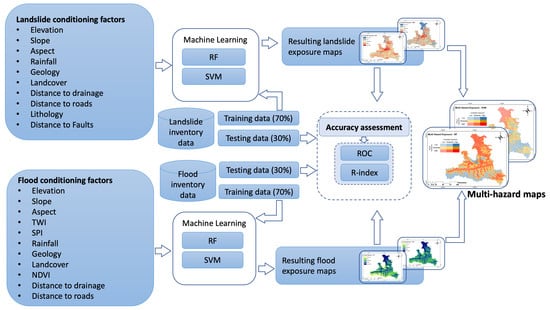
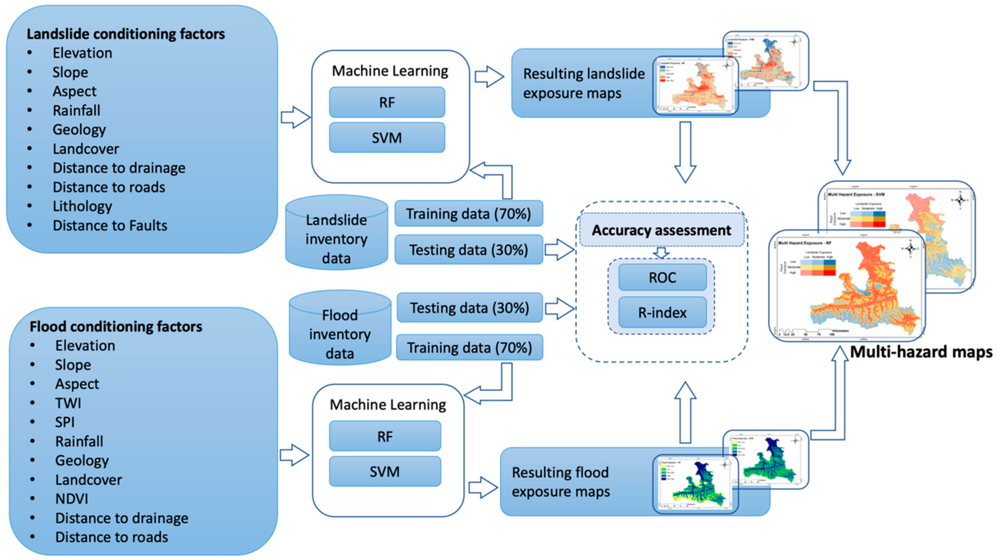
The overall workflow is shown in Figure 4, which shows the influencing factors used for flood and landslide and the ML approaches used for deriving flood and landslide exposure maps.
4. Results
The exposure maps were derived using the machine learning algorithms of RF and SVM for multi-hazard exposure assessments for the State of Salzburg, focusing on floods and landslides. The resultant exposure maps were normalized for both RF and SVM to have consistent classification schema and for comparison. The exposure maps were categorized into five classes of very high, high, moderate, low, and very low exposure levels using the classification schema of the quantile. This quantile classification approach allocates all the values into clusters that comprises an equal number of values for better classification compared to natural break classification schema.
4.1. Flood
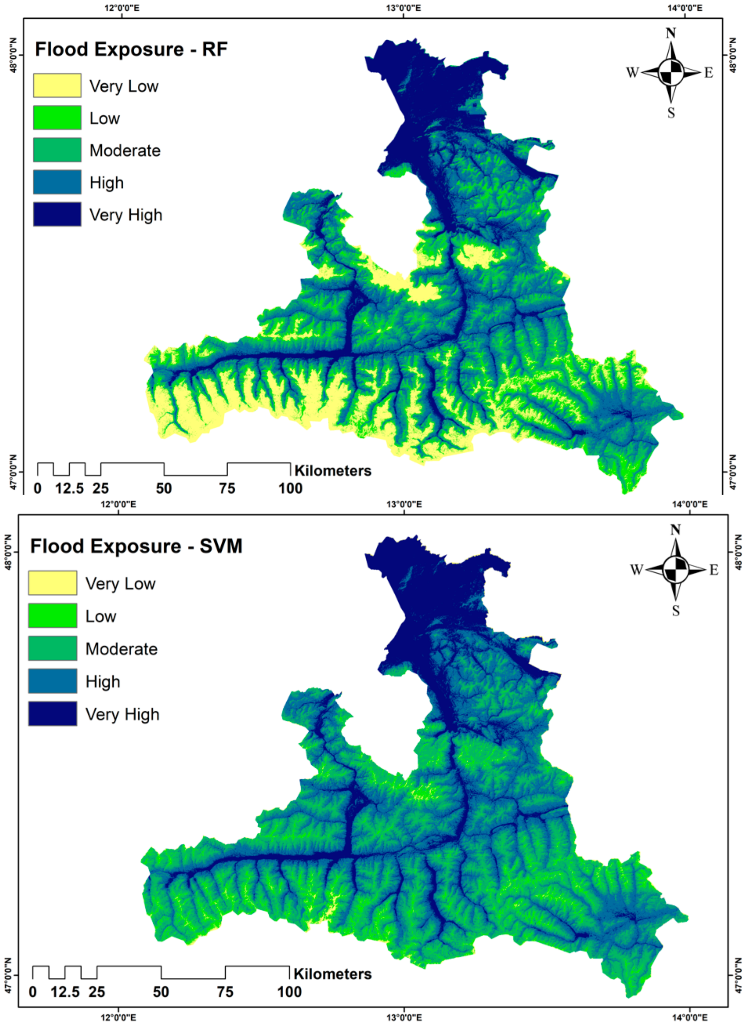
Flood exposure maps were derived for the state of Salzburg in Austria by means of RF and SVM. Overall, the spatial pattern displays north part of the region to be highly susceptible to the flooding and the central region along the Salzach basin to be exposed to flooding, and this is due to the Salzach basin which flows through the region as shown in Figure 5. Both RF and SVM have similar exposure maps except for RF displaying more very low exposure class throughout the region compared to the SVM exposure map. The area wise percentage for each class shows similar percentage for “Very High” exposure class for RF (18%) and SVM (19%) though in the “Very Low” class, RF has 15% compared to 1% in SVM. However other exposure classes also varies compared to RF and SVM as seen in Table 2.
4.2. Landslide
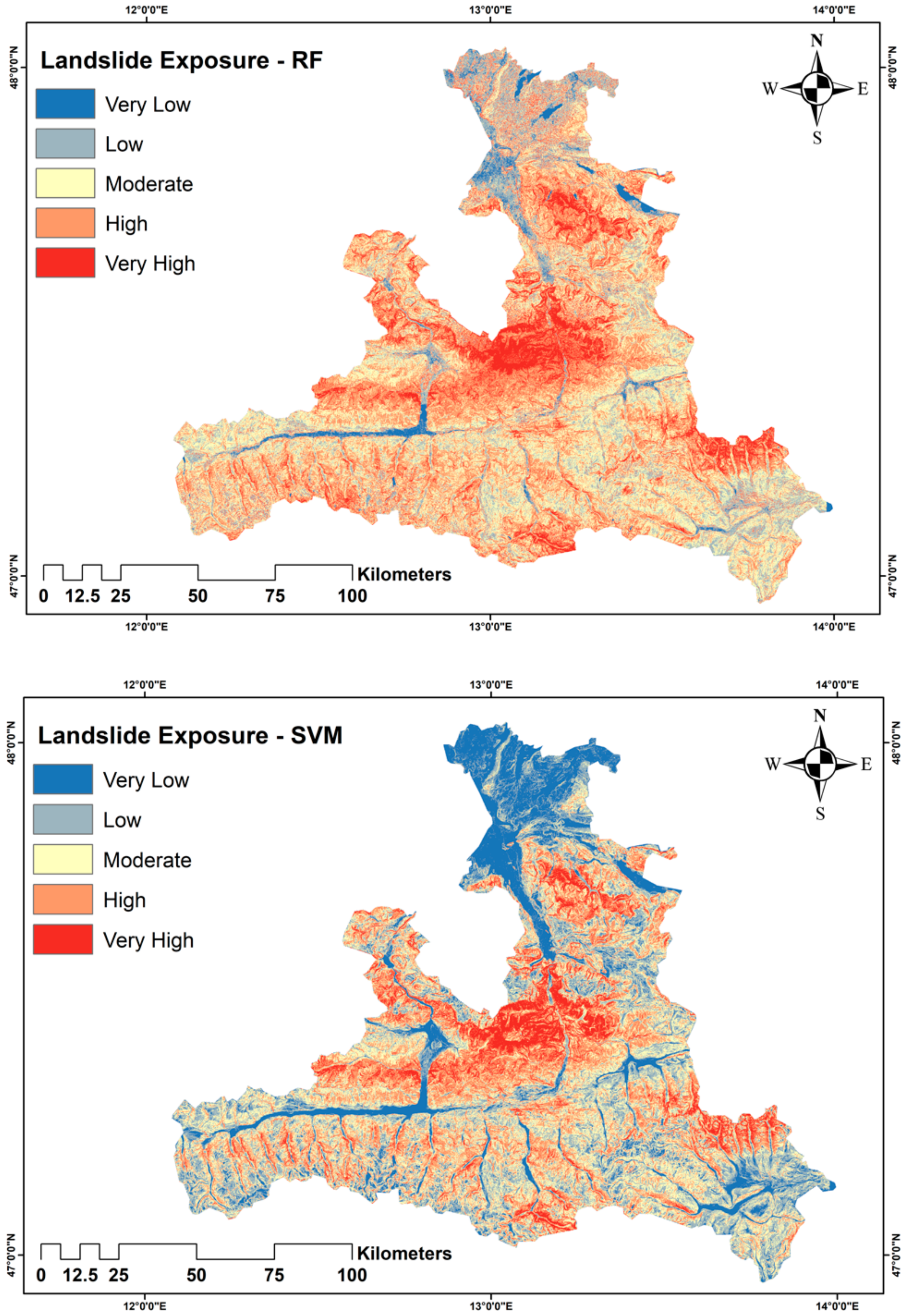
Landslide exposure maps were derived for the State of Salzburg, Austria, using RF and SVM. Overall, the spatial pattern shows central and few northern parts of the region as highly susceptible to the occurrences of landslides. Whereas, SVM shows low occurrences of landslides in the north most areas compared to RF, which shows mixed susceptible regions in the same region, as shown in Figure 6. The area wise percentage for each class displays contrasting percentage for all the exposure classes for RF and SVM.
RF has 14% area that are classified as “Very High” exposure for landslides compared to 9% in SVM, whereas the “Very Low” exposure class area percentage varies considerably between RF (2%) and SVM (16%) which are clearly visible in the derived exposure map shown in Figure 6. The exposure class area percentage is shown for each exposure class derived from RF and SVM for landslides are shown in Table 3.
4.3. Multi-Hazard Exposure Map
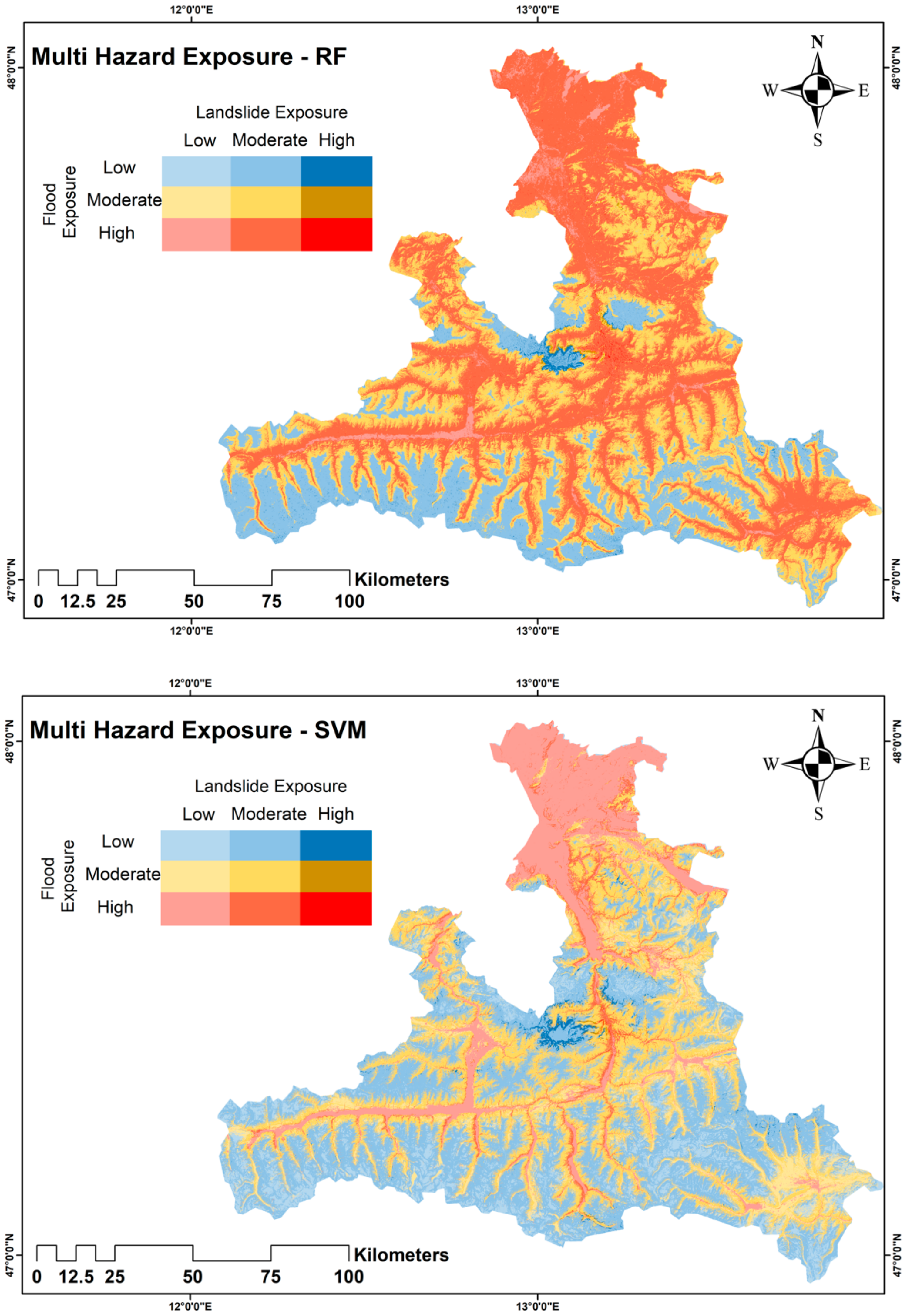
Multi-hazard susceptible maps were derived by the interaction between landslides and floods for the State of Salzburg. The resulting maps show the classification schema of low, moderate, and high susceptible regions as a matrix between floods and landslides. RF shows most of the region as moderate to highly susceptible to both floods and landslides, and the SVM shows the majority of the regions as low susceptible excluding the north part of the region as highly susceptible to floods as shown in Figure 7.
5. Validation
Validation is one of the substantial phases in appraising the precision of every model or technique. Validating the resulting maps stipulates the supremacy of the methodology and its relevance [46]. To establish the accomplishment of the ML models for multi-hazard exposure mapping, a comparison was made among the resulting exposure maps for flood, and landslide derived from SVM and RF using the inventory data for both flood and landslide. To determine the accuracy and efficiency of the model’s analysis of the conformity between the inventory data and the resulting maps specifies if the applied models can correctly envisage the zones that are susceptible to floods and landslides [15]. Thirty percent of the inventory data for each flood and landslide were used for validating the results. There is no commanding standard for allocating inventory data into training and validation data [60]. However, the widely used tactic in literature for natural hazard assessment for classifying the inventory data is known to be 70/30, and hence we have also used the same ratio for splitting the dataset [89].
5.1. Receiver Operating Characteristics (ROC)
The receiver operating characteristics (ROC) curve was derived using the validation inventory for flood and landslides to assess the performance of the RF and SVM models. The ROC method facilitates to establish the precision of each model by comparing the true positive on the vertical axis with the false positive on the horizontal axis from the exposure maps [90]. True positives are the pixels which are rightly categorized as highly exposed to flood/landside and false positives are the pixels that falsely labelled as low exposure to flood/landslide. The area under the curve (AUC) is a grade that stipulates the accurateness of each exposure map outputs. The AUC specifies the likelihood that more pixels were accurately labelled than incorrectly labelled. Higher AUC values indicate a higher accuracy and lower AUC values indicate lower accuracy of the exposure map. If the AUC values are near to unity, then this indicates a significant exposure map. A value of 0.5 shows an inconsequential map since it means the map was produced by accident [91]. Table 4 indicates the AUC intervals with the description.
Figure 8 shows the accuracy of RF and SVM for flood and landslide for the State of Salzburg. The RF yields better accuracy for both flood and landslides compared to SVM though for floods the accuracy of both the models is quite similar. Overall, the accuracy of RF and SVM for flood and landslide is described as good, which is in the range of 0.80–0.90.
5.2. Relative Density (R-Index)
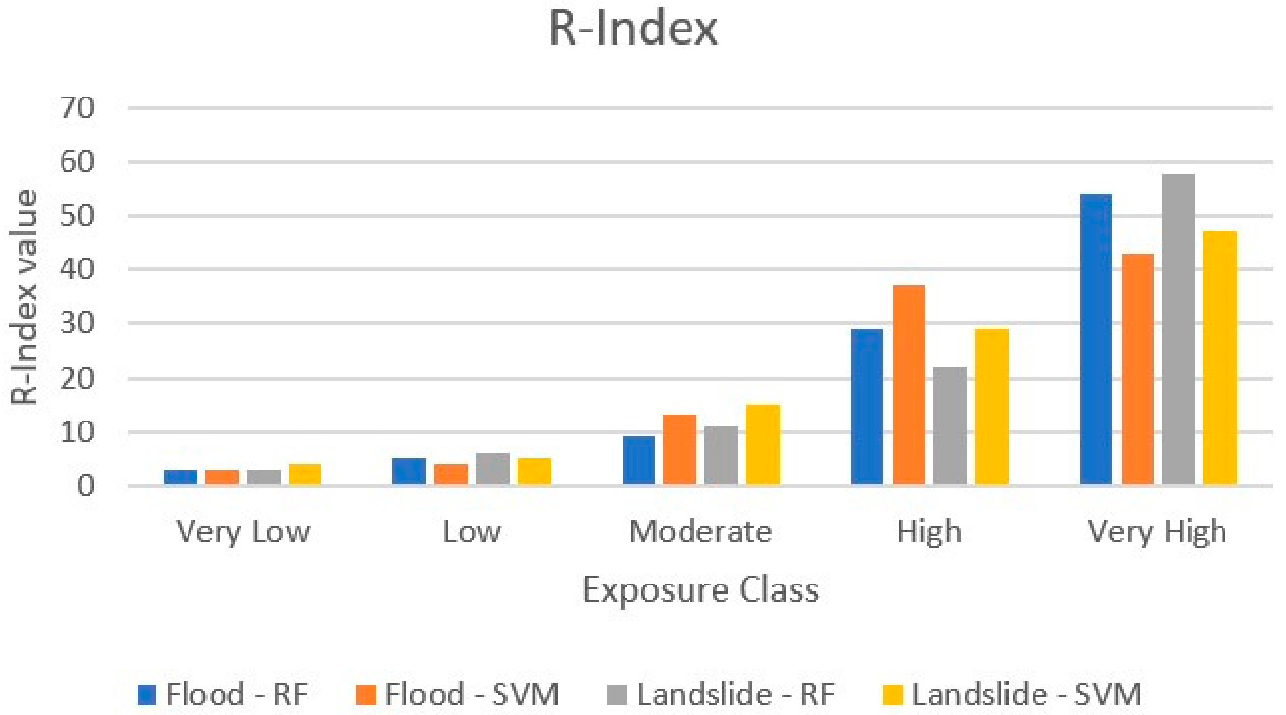
The precision of multi-hazard exposure maps for flood and landslides are assessed using the index of relative density or generally known as the R-Index. This is a common approach used for assessing the area exposed to natural hazards for each of the exposed class. The testing inventory data for flood and landslide was used for authenticating the exposure maps using the equation given below where the ni is defined as the fraction of the particular area that is exposed to floods and landslides for each of the exposed class and Ni is defined as the fraction of the flood and landslide positions in each of the exposed class.
Table 5 displays the r-index for flood and landslide with random forest and support vector machines with the five exposure classes. The r-index illustrates together RF and SVM has the highest values for flood and landslides in the very high exposure class and the lowest in the very low exposure class, as shown in Figure 9.
6. Discussion
Decision support tools such as modelling and simulation increase the awareness and understanding of various hazard managements. Though the configuration and the approaches of modelling differ significantly, this also influences the modelling results and performance of the model. However, the availability of diverse approaches and models presents planners and policymakers to acquire and realize efficient management measures [92]. Various models have been widely used in different hazard assessments like floods, landslide, and wildfire exposure [26,42,78]. Relative and proportional research is desirable to assess the performance of various models in similar conditions with similar influencing factors to make a fair conclusion on the suitable model for a specific hazard at a certain region [93].
This study presents a multi-hazard exposure for flood and landslide hazards for the State of Salzburg, Austria, using ML approaches of RF and SVM. RF is an unpretentious yet fast algorithm that does not utilize any statistical expectations and is illustrated by the high performance that is also evident in this study [94]. In addition, SVM models are known to handle complex, non-linear relationships and are quite insensitive to noise [33]. Both these models have been used for flood and landslide risk assessments. In our study, the RF model yielded similar accuracy for flood and landslides, whereas RF yielded better accuracy results for flood compared to SVM. This might also differ in different regions with different influencing factors used in the study as well. This also shows that both the models yielded better accuracy results for flood and landslide exposure maps and also is in line with previous studies [26,95]. The precision of any model is contingent on the choice of involvement of the chosen influencing factors for natural hazard exposure mapping. The greater amount of influencing features would envisage surging in the precision of the approach. However, this also hangs on the choice and availability of the influencing factor datasets for the region [96]. Furthermore, the superior resolution of datasets selected for the analysis for the study area may also sway the result of exposure maps together with the choice and accessibility of influencing datasets.
The results from the exposure maps derived through RF and SVM shows varying area percentage for the State of Salzburg for flood and landslides as shown in Table 2 and Table 3. Though the flood area percentage for each exposure class is similar to RF and SVM, it varies completely for landslide with totally different area wise percentage for RF and SVM. However the accuracy of the RF shows better results than the SVM and the multi hazard exposure map solves this issue with the exposure class matrix for flood and landslide which shows the region which are highly prone to both floods and landslides and also which region is more exposed to floods and landslides based on the exposure class. Advanced ML methods like feature selection (simulate annealing) with resampling algorithms were also used for flood susceptibility mapping [49]. Previous studies for flood susceptibility shows similar results [42] and the advantage of this study is the multi-hazard exposure map which shows both flood and landslide exposed region based on the matrix. Various other ML approaches like random subspace-based classification and regression tree (RSCART) and logistic regression was used for benchmarking [89], along with the evidence belief function (EBF) model with logistic regression (LR) for landslide susceptibility mapping [97]. There have been studies on landslide susceptibility mappin that uses deep learning convolution neural networks for landslide detection [77] and hybrid integration of EBF and ML approaches [89]. In addition, there are ensemble models which incorporates object based image analysis (OBIA) with ML approaches like multi-layer perceptron neural network (MLP-NN) and random forest (RF) for landslide detection [88]. The recent studies shows the ensemble of radial basis function neural network (RBFN) with random subspace (RSS), attribute selected classifier (ASC), cascade generalization (CG), and dagging for spatial prediction of landslide susceptibility [98].
For future work, ML approaches of RF and SVM can be applied to different geographical settings for the comparison between alpine and mountain region (Nepal and India) where the region is prone to frequent landslides and floods. It will be interesting to evaluate the availability of influencing factors and the suitability to the region as well and to adapt the multi-hazard ML approach for exposure analysis. This would benefit us in the investigation of the robustness of the approaches selected for different geographical venue. The landslide inventory used for this study was point-based landslide locations, and in future, we would like to have the polygon-based inventory where the different approaches can be compared with the influencing factors. We would also like to carry out the multi-hazard vulnerability assessment along with analyzing the interactions between the multi-hazards that will assist in understanding the relationship between the occurrences of these hazards and provides better judgment in the selection of influencing factors.
The exposure maps of multi-hazard for the State of Salzburg provide the planners and disaster management professionals along with the regional authority better management principles for mitigating the hazards in the region. This could also help in preparing detailed measures where there are high susceptible zones for both the hazards rather than planning measures for a single hazard as this could considerably diminish the damages along with the economic losses in the region.
7. Conclusions
Multi-hazard modelling and mapping were conducted based on two natural hazards (landslide and floods) in a hazard-prone region of the State of Salzburg in Austria. Landslides and floods are the most commonly occurring natural hazards in recent years and have caused major indemnities across the selected study area. The SVM and RF ML models were used to model and map hazard-prone areas for both landslide and floods. The resulting of exposure maps of each model and each hazard were then overlapped to produce the multi-hazard exposure maps. The resulting multi-hazard exposure maps provide a better tool for deriving management policies and to identify hazard-prone areas and implement mitigation measures. There have been limited studies carried out for single hazard exposure assessments in the State of Salzburg, and this study is the first of its kind for multi-hazard exposure analysis focusing on floods and landslides which are the two main natural hazards occurring in the region. In this study, we created exposure maps for floods and landslides along with combining these two hazards in yielding a multi-hazard exposure map using RF and SVM algorithms. The precision and the degree of fit of the resultant exposure maps were authenticated using the ROC and R-index. The conclusions and considerations gained from this study provide an enriched understanding of multi-hazard exposure for the State of Salzburg. The mappings assist in recognizing the different exposure classes for the region. This approach can be applied to different regions where multiple natural hazard occurrences are arising in the specific region. The particular results can be advantageous for managers and disaster management to distinguish the areas prone to multi-hazards and to mitigate the economic and financial loss from the natural hazards in the future.
Author Contributions
Conceptualization, T.G.N. and O.G.; Methodology, O.G., T.G.N. and K.G.; Software, K.G., T.G.N. and O.G.; Validation, T.G.N.; Formal Analysis, T.G.N. and O.G.; Investigation, O.G. and T.G.N.; Data Curation, T.G.N.; Writing—Original Draft Preparation, T.G.N.; Writing—Review & Editing, O.G. and T.B.; Visualization, T.G.N. and O.G.; Supervision, T.B.; Funding Acquisition, T.B. All authors have read and agreed to the published version of the manuscript.
Funding
This research was partially funded by the Austrian Science Fund FWF through the GIScience Doctoral College (DK W 1237-N23) at the University of Salzburg.
Acknowledgments
The authors would like to acknowledge the Hochwasserrisikozonierung—Flood risk zoning (HORA), Geological Survey of Austria (GBA) for offering the flood and Landslide data for the research and the Open Access Funding by the Austrian Science Fund (FWF).
Conflicts of Interest
The authors declare no conflict of interest.
References
- Guzzetti, F.; Mondini, A.C.; Cardinali, M.; Fiorucci, F.; Santangelo, M.; Chang, K.-T. Landslide inventory maps: New tools for an old problem. Earth Sci. Rev. 2012, 112, 42–66. [Google Scholar] [CrossRef] [Green Version]
- Bui, D.T.; Khosravi, K.; Shahabi, H.; Daggupati, P.; Adamowski, J.F.; Melesse, A.M.; Pham, B.T.; Pourghasemi, H.R.; Mahmoudi, M.; Bahrami, S.; et al. Flood Spatial Modeling in Northern Iran Using Remote Sensing and GIS: A Comparison between Evidential Belief Functions and Its Ensemble with a Multivariate Logistic Regression Model. Remote Sens. 2019, 11, 1589. [Google Scholar] [CrossRef] [Green Version]
- UNEP. Technical Report United on Agenda 21. Available online: https://www.un.org/esa/dsd/agenda21/res_agenda21_07.shtml (accessed on 20 July 2020).
- Pourghasemi, H.R.; Gayen, A.; Edalat, M.; Zarafshar, M.; Tiefenbacher, J.P. Is multi-hazard mapping effective in assessing natural hazards and integrated watershed management? Geosci. Front. 2020, 11, 1203–1217. [Google Scholar] [CrossRef]
- Kalantari, Z.; Ferreira, C.S.S.; Koutsouris, A.J.; Ahlmer, A.-K.; Cerdà, A.; Destouni, G.; Ahmer, A.-K. Assessing flood probability for transportation infrastructure based on catchment characteristics, sediment connectivity and remotely sensed soil moisture. Sci. Total Environ. 2019, 661, 393–406. [Google Scholar] [CrossRef] [PubMed]
- Hirabayashi, Y.; Mahendran, R.; Koirala, S.; Konoshima, L.; Yamazaki, D.; Watanabe, S.; Kim, H.; Kanae, S. Global flood risk under climate change. Nat. Clim. Chang. 2013, 3, 816–821. [Google Scholar] [CrossRef]
- Wang, Y.; Hong, H.; Chen, W.; Li, S.; Panahi, M.; Khosravi, K.; Shirzadi, A.; Shahabi, H.; Panahi, S.; Costache, R. Flood susceptibility mapping in Dingnan County (China) using adaptive neuro-fuzzy inference system with biogeography based optimization and imperialistic competitive algorithm. J. Environ. Manag. 2019, 247, 712–729. [Google Scholar] [CrossRef]
- Khosravi, K.; Shahabi, H.; Pham, B.T.; Adamowski, J.; Shirzadi, A.; Pradhan, B.; Dou, J.; Ly, H.B.; Grof, G.H.; Ho, L.; et al. A comparative assessment of flood susceptibility modeling using multi-criteria decision-making analysis and machine learning methods. J. Hydrol. 2019, 573, 311–323. [Google Scholar] [CrossRef]
- Shahabi, H.; Shirzadi, A.; Ghaderi, K.; Omidavr, E.; Al-Ansari, N.; Clague, J.J.; Geertsema, M.; Khosravi, K.; Amini, A.; Bahrami, S.; et al. Flood Detection and Susceptibility Mapping Using Sentinel-1 Remote Sensing Data and a Machine Learning Approach: Hybrid Intelligence of Bagging Ensemble Based on K-Nearest Neighbor Classifier. Remote Sens. 2020, 12, 266. [Google Scholar] [CrossRef] [Green Version]
- Yu, J.J.; Qin, X.; Larsen, O. Joint Monte Carlo and possibilistic simulation for flood damage assessment. Stoch. Environ. Res. Risk Assess. 2012, 27, 725–735. [Google Scholar] [CrossRef]
- Ligtvoet, W.; Witte, F.; Goldschmidt, T.; Van Oijen, M.; Wanink, J.; Goudswaard, P. Species Extinction and Concomitant Ecological Changes in Lake Victoria. Neth. J. Zoöl. 1991, 42, 214–232. [Google Scholar] [CrossRef] [Green Version]
- Markantonis, V.; Meyer, V.; Lienhoop, N. Evaluation of the environmental impacts of extreme floods in the evros river basin using contingent valuation method. Nat. Hazards 2013, 69, 1535–1549. [Google Scholar] [CrossRef]
- Clerici, A.; Perego, S.; Tellini, C.; Vescovi, P. A procedure for landslide susceptibility zonation by the conditional analysis method. Geomorphology 2002, 48, 349–364. [Google Scholar] [CrossRef]
- Wilde, M.; Günther, A.; Reichenbach, P.; Malet, J.-P.; Hervas, J. Pan-European landslide susceptibility mapping: ELSUS Version 2. J. Maps 2018, 14, 97–104. [Google Scholar] [CrossRef] [Green Version]
- Pourghasemi, H.R.; Rahmati, O. Prediction of the landslide susceptibility: Which algorithm, which precision? Catena 2018, 162, 177–192. [Google Scholar] [CrossRef]
- Li, R.; Wang, N. Landslide Susceptibility Mapping for the Muchuan County (China): A Comparison Between Bivariate Statistical Models (WoE, EBF, and IoE) and Their Ensembles with Logistic Regression. Symmetry 2019, 11, 762. [Google Scholar] [CrossRef] [Green Version]
- Gordo, C.; Zêzere, J.L.; Marques, R. Landslide Susceptibility Assessment at the Basin Scale for Rainfall- and Earthquake-Triggered Shallow Slides. Geosciences 2019, 9, 268. [Google Scholar] [CrossRef] [Green Version]
- Lima, P.H.; Steger, S.; Glade, T.; Tilch, N.; Schwarz, L.; Kociu, A.; Mikoš, M.; Tiwari, B.; Yin, Y.; Sassa, K. Landslide Susceptibility Mapping at National Scale: A First Attempt for Austria. Adv. Cult. Living Landslides 2017, 943–951. [Google Scholar] [CrossRef]
- Sachdeva, S.; Bhatia, T.; Verma, A.K. Flood susceptibility mapping using GIS-based support vector machine and particle swarm optimization: A case study in Uttarakhand (India). In Proceedings of the 2017 8th International Conference on Computing, Communication and Networking Technologies (ICCCNT), Delhi, India, 3–5 July 2017; pp. 1–7. [Google Scholar]
- Hong, H.; Pradhan, B.; Xu, C.; Bui, D.T. Spatial prediction of landslide hazard at the Yihuang area (China) using two-class kernel logistic regression, alternating decision tree and support vector machines. Catena 2015, 133, 266–281. [Google Scholar] [CrossRef]
- Rahmati, O.; Pourghasemi, H.R.; Zeinivand, H. Flood susceptibility mapping using frequency ratio and weights-of-evidence models in the Golastan Province, Iran. Geocarto Int. 2015, 31, 42–70. [Google Scholar] [CrossRef]
- Yariyan, P.; Avand, M.; Abbaspour, R.A.; Karami, M.; Tiefenbacher, J.P. GIS-based spatial modeling of snow avalanches using four novel ensemble models. Sci. Total Environ. 2020, 745, 141008. [Google Scholar] [CrossRef]
- Rahmati, O.; Zeinivand, H.; Besharat, M. Flood hazard zoning in Yasooj region, Iran, using GIS and multi-criteria decision analysis. Geomatics Nat. Hazards Risk 2015, 7, 1000–1017. [Google Scholar] [CrossRef] [Green Version]
- Shahabi, H.; Khezri, S.; Ahmed, B.; Hashim, M. Landslide susceptibility mapping at central Zab basin, Iran: A comparison between analytical hierarchy process, frequency ratio and logistic regression models. Catena 2014, 115, 55–70. [Google Scholar] [CrossRef]
- Pirnazar, M.; Karimi, A.Z.; Feizizadeh, B.; Ostad-Ali-Askari, K.; Eslamian, S.; Hasheminasab, H.; Ghorbanzadeh, O.; Hamedani, M.H. Assessing flood hazard using gis based multi-criteria decision making approach. Study area: East-Azerbaijan province (Kaleybar Chay basin). J. Flood Eng. 2017, 8, 203–223. [Google Scholar]
- Tehrany, M.S.; Pradhan, B.; Jebur, M.N. Flood susceptibility analysis and its verification using a novel ensemble support vector machine and frequency ratio method. Stoch. Environ. Res. Risk Assess. 2015, 29, 1149–1165. [Google Scholar] [CrossRef]
- Panahi, M.; Sadhasivam, N.; Pourghasemi, H.R.; Rezaie, F.; Lee, S. Spatial prediction of groundwater potential mapping based on convolutional neural network (CNN) and support vector regression (SVR). J. Hydrol. 2020, 588, 125033. [Google Scholar] [CrossRef]
- Chapi, K.; Singh, V.P.; Shirzadi, A.; Shahabi, H.; Bui, D.T.; Pham, B.T.; Khosravi, K. A novel hybrid artificial intelligence approach for flood susceptibility assessment. Environ. Model. Softw. 2017, 95, 229–245. [Google Scholar] [CrossRef]
- Nampak, H.; Pradhan, B.; Manap, M.A. Application of GIS based data driven evidential belief function model to predict groundwater potential zonation. J. Hydrol. 2014, 513, 283–300. [Google Scholar] [CrossRef]
- Rahmati, O.; Panahi, M.; Ghiasi, S.S.; Deo, R.C.; Tiefenbacher, J.P.; Pradhan, B.; Jahani, A.; Goshtasb, H.; Kornejady, A.; Shahabi, H.; et al. Hybridized neural fuzzy ensembles for dust source modeling and prediction. Atmos. Environ. 2020, 224, 117320. [Google Scholar] [CrossRef]
- Ghorbanzadeh, O.; Rostamzadeh, H.; Blaschke, T.; Gholaminia, K.; Aryal, J. A new gis-based data mining technique using an adaptive neuro-fuzzy inference system (anfis) and k-fold cross-validation approach for land subsidence susceptibility mapping. Nat. Hazards 2018, 94, 497–517. [Google Scholar] [CrossRef] [Green Version]
- Mohammady, M.; Pourghasemi, H.R.; Pradhan, B. Landslide susceptibility mapping at golestan province, iran: A comparison between frequency ratio, dempster-shafer, and weights-of-evidence models. J. Asian Earth Sci. 2012, 61, 221–236. [Google Scholar] [CrossRef]
- Pourghasemi, H.; Pradhan, B.; Gokceoglu, C.; Moezzi, K.D. A comparative assessment of prediction capabilities of dempster-shafer and weights-of-evidence models in landslide susceptibility mapping using gis. Geomat. Nat. Hazards Risk 2013, 4, 93–118. [Google Scholar] [CrossRef]
- Tehrany, M.S.; Pradhan, B.; Jebur, M.N. Spatial prediction of flood susceptible areas using rule based decision tree (dt) and a novel ensemble bivariate and multivariate statistical models in gis. J. Hydrol. 2013, 504, 69–79. [Google Scholar] [CrossRef]
- Khosravi, K.; Pham, B.T.; Chapi, K.; Shirzadi, A.; Shahabi, H.; Revhaug, I.; Prakash, I.; Bui, D.T. A comparative assessment of decision trees algorithms for flash flood susceptibility modeling at Haraz watershed, northern Iran. Sci. Total Environ. 2018, 627, 744–755. [Google Scholar] [CrossRef] [PubMed]
- Lee, S.; Pradhan, B.; Mansor, S.; Buchroithner, M.; Jamaluddin, N.; Khujaimah, Z. Utilization of optical remote sensing data and geographic information system tools for regional landslide hazard analysis by using binomial logistic regression model. J. Appl. Remote Sens. 2008, 2, 023542. [Google Scholar] [CrossRef]
- Felicísimo, Á.M.; Cuartero, A.; Remondo, J.; Quirós, E.; Felicísimo, A.M. Mapping landslide susceptibility with logistic regression, multiple adaptive regression splines, classification and regression trees, and maximum entropy methods: A comparative study. Landslides 2012, 10, 175–189. [Google Scholar] [CrossRef]
- Ghorbanzadeh, O.; Blaschke, T.; Gholamnia, K.; Aryal, J. Forest Fire Susceptibility and Risk Mapping Using Social/Infrastructural Vulnerability and Environmental Variables. Fire 2019, 2, 50. [Google Scholar] [CrossRef] [Green Version]
- Ngo, P.-T.T.; Panahi, M.; Khosravi, K.; Ghorbanzadeh, O.; Karimnejad, N.; Cerda, A.; Lee, S. Evaluation of deep learning algorithms for national scale landslide susceptibility mapping of Iran. Geosci. Front. 2020. [Google Scholar] [CrossRef]
- Jaafari, A.; Zenner, E.K.; Panahi, M.; Shahabi, H. Hybrid artificial intelligence models based on a neuro-fuzzy system and metaheuristic optimization algorithms for spatial prediction of wildfire probability. Agric. For. Meteorol. 2019, 266–267, 198–207. [Google Scholar] [CrossRef]
- Ghorbanzadeh, O.; Kamran, K.; Blaschke, T.; Aryal, J.; Naboureh, A.; Einali, J.; Bian, J. Spatial Prediction of Wildfire Susceptibility Using Field Survey GPS Data and Machine Learning Approaches. Fire 2019, 2, 43. [Google Scholar] [CrossRef] [Green Version]
- Nachappa, T.G.; Piralilou, S.T.; Gholamnia, K.; Ghorbanzadeh, O.; Rahmati, O.; Blaschke, T. Flood susceptibility mapping with machine learning, multi-criteria decision analysis and ensemble using Dempster Shafer Theory. J. Hydrol. 2020, 590, 125275. [Google Scholar] [CrossRef]
- Rahmati, O.; Yousefi, S.; Kalantari, Z.; Uuemaa, E.; Teimurian, T.; Keesstra, S.D.; Pham, T.; Bui, D.T. Multi-Hazard Exposure Mapping Using Machine Learning Techniques: A Case Study from Iran. Remote Sens. 2019, 11, 1943. [Google Scholar] [CrossRef] [Green Version]
- Kappes, M.S.; Keiler, M.; Von Elverfeldt, K.; Glade, T. Challenges of analyzing multi-hazard risk: A review. Nat. Hazards 2012, 64, 1925–1958. [Google Scholar] [CrossRef] [Green Version]
- Khosravi, K.; Panahi, M.; Bui, D.T. Spatial prediction of groundwater spring potential mapping based on an adaptive neuro-fuzzy inference system and metaheuristic optimization. Hydrol. Earth Syst. Sci. 2018, 22, 4771–4792. [Google Scholar] [CrossRef] [Green Version]
- Arabameri, A.; Rezaei, K.; Cerdà, A.; Conoscenti, C.; Kalantari, Z. A comparison of statistical methods and multi-criteria decision making to map flood hazard susceptibility in Northern Iran. Sci. Total Environ. 2019, 660, 443–458. [Google Scholar] [CrossRef]
- Chowdhuri, I.; Pal, S.C.; Chakrabortty, R. Flood susceptibility mapping by ensemble evidential belief function and binomial logistic regression model on river basin of eastern India. Adv. Space Res. 2020, 65, 1466–1489. [Google Scholar] [CrossRef]
- Mosavi, A.; Ozturk, P.; Chau, K.-W. Flood Prediction Using Machine Learning Models: Literature Review. Water 2018, 10, 1536. [Google Scholar] [CrossRef] [Green Version]
- Hosseini, F.S.; Choubin, B.; Mosavi, A.; Nabipour, N.; Shamshirband, S.; Darabi, H.; Haghighi, A.T. Flash-flood hazard assessment using ensembles and Bayesian-based machine learning models: Application of the simulated annealing feature selection method. Sci. Total Environ. 2020, 711, 135161. [Google Scholar] [CrossRef]
- Ghorbanzadeh, O.; Blaschke, T. Optimizing Sample Patches Selection of CNN to Improve the mIOU on Landslide Detection. In Proceedings of the 5th International Conference on Geographical Information Systems Theory, Applications and Management, Heraklion, Crete, Greece, 3–5 May 2019; pp. 33–40. [Google Scholar]
- Mezaal, M.R.; Pradhan, B.; Rizeei, H.M. Improving Landslide Detection from Airborne Laser Scanning Data Using Optimized Dempster–Shafer. Remote Sens. 2018, 10, 1029. [Google Scholar] [CrossRef] [Green Version]
- Nachappa, T.G.; Piralilou, S.T.; Ghorbanzadeh, O.; Shahabi, H.; Blaschke, T. Landslide Susceptibility Mapping for Austria Using Geons and Optimization with the Dempster-Shafer Theory. Appl. Sci. 2019, 9, 5393. [Google Scholar] [CrossRef] [Green Version]
- Fuchs, S.; Keiler, M.; Zischg, A.P. A spatiotemporal multi-hazard exposure assessment based on property data. Nat. Hazards Earth Syst. Sci. 2015, 15, 2127–2142. [Google Scholar] [CrossRef] [Green Version]
- Fuchs, S.; Keiler, M.; Sokratov, S.A.; Shnyparkov, A. Spatiotemporal dynamics: The need for an innovative approach in mountain hazard risk management. Nat. Hazards 2012, 68, 1217–1241. [Google Scholar] [CrossRef]
- Nachappa, T.G.; Kienberger, S.; Meena, S.R.; Hölbling, D.; Blaschke, T. Comparison and validation of per-pixel and object-based approaches for landslide susceptibility mapping. Geomat. Nat. Hazards Risk 2020, 11, 572–600. [Google Scholar]
- Höller, P. Avalanche cycles in Austria: An analysis of the major events in the last 50 years. Nat. Hazards 2008, 48, 399–424. [Google Scholar] [CrossRef]
- Kundzewicz, Z.W.; Lugeri, N.; Dankers, R.; Hirabayashi, Y.; Doll, P.; Pińskwar, I.; Dysarz, T.; Hochrainer, S.; Matczak, P. Assessing river flood risk and adaptation in Europe—Review of projections for the future. Mitig. Adapt. Strat. Glob. Chang. 2010, 15, 641–656. [Google Scholar] [CrossRef]
- Gobiet, A.; Kotlarski, S.; Beniston, M.; Heinrich, G.; Rajczak, J.; Stoffel, M. 21st century climate change in the European Alps—A review. Sci. Total Environ. 2014, 493, 1138–1151. [Google Scholar] [CrossRef]
- Khosravi, K.; Nohani, E.; Maroufinia, E.; Pourghasemi, H.R. A GIS-based flood susceptibility assessment and its mapping in Iran: A comparison between frequency ratio and weights-of-evidence bivariate statistical models with multi-criteria decision-making technique. Nat. Hazards 2016, 83, 947–987. [Google Scholar] [CrossRef]
- Tsangaratos, P.; Ilia, I. Comparison of a logistic regression and Naïve Bayes classifier in landslide susceptibility assessments: The influence of models complexity and training dataset size. Catena 2016, 145, 164–179. [Google Scholar] [CrossRef]
- Umar, Z.; Pradhan, B.; Ahmad, A.; Jebur, M.N.; Tehrany, M.S. Earthquake induced landslide susceptibility mapping using an integrated ensemble frequency ratio and logistic regression models in West Sumatera Province, Indonesia. Catena 2014, 118, 124–135. [Google Scholar] [CrossRef]
- Kumar, R.; Anbalagan, R. Landslide susceptibility mapping using analytical hierarchy process (AHP) in Tehri reservoir rim region, Uttarakhand. J. Geol. Soc. India 2016, 87, 271–286. [Google Scholar] [CrossRef]
- Raja, N.B.; Çiçek, I.; Türkoğlu, N.; Aydin, O.; Kawasaki, A.; Ciçek, I.; Aydın, O. Correction to: Landslide susceptibility mapping of the Sera River Basin using logistic regression model. Nat. Hazards 2017, 91, 1423. [Google Scholar] [CrossRef] [Green Version]
- Youssef, A.M.; Pradhan, B.; Hassan, A.M. Flash flood risk estimation along the St. Katherine road, southern Sinai, Egypt using GIS based morphometry and satellite imagery. Environ. Earth Sci. 2010, 62, 611–623. [Google Scholar] [CrossRef]
- Pham, B.T.; Prakash, I.; Khosravi, K.; Chapi, K.; Trinh, P.T.; Ngo, T.Q.; Hosseini, S.V.; Bui, D.T. A comparison of Support Vector Machines and Bayesian algorithms for landslide susceptibility modelling. Geocarto Int. 2018, 34, 1385–1407. [Google Scholar] [CrossRef]
- Mohammadi, A.; Shahabi, H.; Ahmad, B.B. Land-cover change detection in a part of cameron highlands, Malaysia using ETM+ satellite imagery and support vector machine (SVM) algorithm. Environ. Asia 2019, 12, 145–154. [Google Scholar] [CrossRef]
- Persichillo, M.G.; Bordoni, M.; Meisina, C. The role of land use changes in the distribution of shallow landslides. Sci. Total Environ. 2017, 574, 924–937. [Google Scholar] [CrossRef] [PubMed]
- Wu, Y.; Li, W.; Wang, Q.; Liu, Q.; Yang, D.; Xing, M.; Pei, Y.; Yan, S. Landslide susceptibility assessment using frequency ratio, statistical index and certainty factor models for the Gangu County, China. Arab. J. Geosci. 2016, 9, 84. [Google Scholar] [CrossRef]
- Chen, W.; Pourghasemi, H.R.; Naghibi, S.A. A comparative study of landslide susceptibility maps produced using support vector machine with different kernel functions and entropy data mining models in China. Bull. Int. Assoc. Eng. Geol. 2017, 77, 647–664. [Google Scholar] [CrossRef]
- Kalantari, Z.; Nickman, A.; Lyon, S.W.; Olofsson, B.; Folkeson, L. A method for mapping flood hazard along roads. J. Environ. Manag. 2014, 133, 69–77. [Google Scholar] [CrossRef] [PubMed]
- Lee, S.; Pradhan, B. Landslide hazard mapping at Selangor, Malaysia using frequency ratio and logistic regression models. Landslides 2006, 4, 33–41. [Google Scholar] [CrossRef]
- Yalcin, A.; Bulut, F. Landslide susceptibility mapping using GIS and digital photogrammetric techniques: A case study from Ardesen (NE-Turkey). Nat. Hazards 2006, 41, 201–226. [Google Scholar] [CrossRef]
- Gokceoglu, C.; Sonmez, H.; Nefeslioglu, H.A.; Duman, T.Y.; Can, T. The 17 March 2005 Kuzulu landslide (Sivas, Turkey) and landslide-susceptibility map of its near vicinity. Eng. Geol. 2005, 81, 65–83. [Google Scholar] [CrossRef]
- Moore, I.D.; Grayson, R.B.; Ladson, A. Digital terrain modelling: A review of hydrological, geomorphological, and biological applications. Hydrol. Process. 1991, 5, 3–30. [Google Scholar] [CrossRef]
- Beven, K.J.; Kirkby, M.J. A physically based, variable contributing area model of basin hydrology / Un modèle à base physique de zone d’appel variable de l’hydrologie du bassin versant. Hydrol. Sci. Bull. 1979, 24, 43–69. [Google Scholar] [CrossRef] [Green Version]
- Shahabi, H. Detection of urban irregular development and green space destruction using normalized difference vegetation index (NDVI), principal component analysis (PCA) and post classification methods: A case study of Saqqez city. Int. J. Phys. Sci. 2012, 7, 2587–2595. [Google Scholar] [CrossRef]
- Ghorbanzadeh, O.; Blaschke, T.; Gholamnia, K.; Meena, S.R.; Tiede, D.; Aryal, J. Evaluation of Different Machine Learning Methods and Deep-Learning Convolutional Neural Networks for Landslide Detection. Remote Sens. 2019, 11, 196. [Google Scholar] [CrossRef] [Green Version]
- Gholamnia, K.; Nachappa, T.G.; Ghorbanzadeh, O.; Blaschke, T. Comparisons of Diverse Machine Learning Approaches for Wildfire Susceptibility Mapping. Symmetry 2020, 12, 604. [Google Scholar] [CrossRef] [Green Version]
- Merghadi, A.; Yunus, A.P.; Dou, J.; Whiteley, J.; ThaiPham, B.; Bui, D.T.; Avtar, R.; Abderrahmane, B. Machine learning methods for landslide susceptibility studies: A comparative overview of algorithm performance. Earth Sci. Rev. 2020, 207, 103225. [Google Scholar] [CrossRef]
- Vapnik, V. The Nature of Statistical Learning Theory; Springer Science & Business Media: Berlin, Germany, 2013. [Google Scholar]
- Kavzoglu, T.; Sahin, E.K.; Colkesen, I. Landslide susceptibility mapping using GIS-based multi-criteria decision analysis, support vector machines, and logistic regression. Landslides 2013, 11, 425–439. [Google Scholar] [CrossRef]
- Bui, D.T.; Tuan, T.A.; Klempe, H.; Pradhan, B.; Revhaug, I. Spatial prediction models for shallow landslide hazards: A comparative assessment of the efficacy of support vector machines, artificial neural networks, kernel logistic regression, and logistic model tree. Landslides 2015, 13, 361–378. [Google Scholar] [CrossRef]
- Schölkopf, B.; Smola, A.J.; Bach, F. Learning with Kernels: Support Vector Machines, Regularization, Optimization, and Beyond; MIT Press: Cambridge, MA, USA, 2002. [Google Scholar]
- Ho, T.K. Random decision forests. In Proceedings of the 3rd International Conference on Document Analysis and Recognition, Montreal, QC, Canada, 14–16 August 1995; Volume 1, pp. 278–282. [Google Scholar]
- Du, P.; Samat, A.; Waske, B.; Liu, S.; Li, Z. Random Forest and Rotation Forest for fully polarized SAR image classification using polarimetric and spatial features. ISPRS J. Photogramm. Remote Sens. 2015, 105, 38–53. [Google Scholar] [CrossRef]
- Xu, R.; Lin, H.; Lü, Y.; Luo, Y.; Ren, Y.; Comber, A. A Modified Change Vector Approach for Quantifying Land Cover Change. Remote Sens. 2018, 10, 1578. [Google Scholar] [CrossRef] [Green Version]
- Valdez, M.C.; Chang, K.-T.; Chen, C.-F.; Chiang, S.-H.; Santos, J.L. Modelling the spatial variability of wildfire susceptibility in Honduras using remote sensing and geographical information systems. Geomatics Nat. Hazards Risk 2017, 8, 876–892. [Google Scholar] [CrossRef] [Green Version]
- Piralilou, S.T.; Shahabi, H.; Jarihani, B.; Ghorbanzadeh, O.; Blaschke, T.; Gholamnia, K.; Meena, S.R.; Aryal, J. Landslide Detection Using Multi-Scale Image Segmentation and Different Machine Learning Models in the Higher Himalayas. Remote Sens. 2019, 11, 2575. [Google Scholar] [CrossRef] [Green Version]
- Li, Y.; Chen, W. Landslide Susceptibility Evaluation Using Hybrid Integration of Evidential Belief Function and Machine Learning Techniques. Water 2019, 12, 113. [Google Scholar] [CrossRef] [Green Version]
- Linden, A. Measuring diagnostic and predictive accuracy in disease management: An introduction to receiver operating characteristic (ROC) analysis. J. Eval. Clin. Pract. 2006, 12, 132–139. [Google Scholar] [CrossRef] [PubMed]
- Baird, C.; Healy, T.; Johnson, K.; Bogie, A.; Dankert, E.W.; Scharenbroch, C. A Comparison of Risk Assessment Instruments in Juvenile Justice; National Council on Crime and Delinquency: Madison, WI, USA, 2013. [Google Scholar]
- Hill, D.J.; Minsker, B.S. Anomaly detection in streaming environmental sensor data: A data-driven modeling approach. Environ. Model. Softw. 2010, 25, 1014–1022. [Google Scholar] [CrossRef]
- Goetz, J.; Brenning, A.; Petschko, H.; Leopold, P. Evaluating machine learning and statistical prediction techniques for landslide susceptibility modeling. Comput. Geosci. 2015, 81, 1–11. [Google Scholar] [CrossRef]
- Pourghasemi, H.R.; Kariminejad, N.; Amiri, M.; Edalat, M.; Zarafshar, M.; Blaschke, T.; Cerdà, A. Assessing and mapping multi-hazard risk susceptibility using a machine learning technique. Sci. Rep. 2020, 10, 1–11. [Google Scholar] [CrossRef] [Green Version]
- Rahmati, O.; Pourghasemi, H.R. Identification of Critical Flood Prone Areas in Data-Scarce and Ungauged Regions: A Comparison of Three Data Mining Models. Water Resour. Manag. 2017, 31, 1473–1487. [Google Scholar] [CrossRef]
- Donati, L.; Turrini, M. An objective method to rank the importance of the factors predisposing to landslides with the GIS methodology: Application to an area of the Apennines (Valnerina; Perugia, Italy). Eng. Geol. 2002, 63, 277–289. [Google Scholar] [CrossRef]
- Zhao, X.; Chen, W. Optimization of Computational Intelligence Models for Landslide Susceptibility Evaluation. Remote Sens. 2020, 12, 2180. [Google Scholar] [CrossRef]
- Pham, B.T.; Nguyen-Thoi, T.; Qi, C.; Van Phong, T.; Dou, J.; Ho, L.S.; Van Le, H.; Prakash, I. Coupling RBF neural network with ensemble learning techniques for landslide susceptibility mapping. Catena 2020, 195, 104805. [Google Scholar] [CrossRef]
Figure 1.
Location of the State of Salzburg, Austria.

Figure 2.
The State of Salzburg showing the flood and landslide inventory divided into training and testing data.
Figure 2.
The State of Salzburg showing the flood and landslide inventory divided into training and testing data.

Figure 3.
Influencing factors for landslides and floods used in this study: (a) elevation (m), (b) slope, (c) aspect, (d) normalized difference vegetation index (NDVI), (e) topographic wetness index (TWI), (f) stream power index (SPI), (g) geology, (h) land cover, (i) distance to drainage (m), (j) distance to road (m), (k) rainfall, (l) distance to fault, and (m) lithology.


Figure 4.
The methodological workflow used for the multi-hazard exposure mapping for the State of Salzburg.
Figure 4.
The methodological workflow used for the multi-hazard exposure mapping for the State of Salzburg.

Figure 5.
Flood exposure maps derived using random forest (RF) and support vector machine (SVM) for the State of Salzburg.
Figure 5.
Flood exposure maps derived using random forest (RF) and support vector machine (SVM) for the State of Salzburg.

Figure 6.
Landslide exposure maps derived using random forest (RF) and support vector machine (SVM) for the State of Salzburg.
Figure 6.
Landslide exposure maps derived using random forest (RF) and support vector machine (SVM) for the State of Salzburg.

Figure 7.
Integrated multi-hazard exposure classification combining flood and landslide using random forest and support vector machine for the State of Salzburg.
Figure 7.
Integrated multi-hazard exposure classification combining flood and landslide using random forest and support vector machine for the State of Salzburg.

Figure 8.
Accuracy of each model with AUC values for flood and landslide using RF and SVM.

Figure 9.
R-index values for flood and landslide using RF and SVM.


Table 1.
Influencing factors for flood and landslides selected for the State of Salzburg.
| Factors | Flood Influencing Factors | Landslides Influencing Factors |
|---|---|---|
| Elevation |  | |
| Slope | | |
| Aspect | | |
| Land cover | | |
| Rainfall | | |
| Geology | | |
| Distance to roads | | |
| Distance to drainage | | |
| NDVI 1 | |  |
| TWI 2 | | |
| SPI 3 | | |
| Lithology | | |
| Distance to faults | | |
1 Normalized difference vegetation index (NDVI); 2 topographic wetness index (TWI); 3 stream power index (SPI).
Table 2.
Area percentage for each exposure class for flood using RF and SVM for the State of Salzburg.
Table 2.
Area percentage for each exposure class for flood using RF and SVM for the State of Salzburg.
| Exposure Class | RF (Area in %) | SVM (Area in %) |
|---|---|---|
| Very Low | 15 | 1 |
| Low | 15 | 8 |
| Moderate | 21 | 36 |
| High | 31 | 36 |
| Very High | 18 | 19 |
Table 3.
Area percentage for each exposure class for landslides using RF and SVM for the State of Salzburg.
Table 3.
Area percentage for each exposure class for landslides using RF and SVM for the State of Salzburg.
| Exposure Class | RF (Area in %) | SVM (Area in %) |
|---|---|---|
| Very Low | 2 | 16 |
| Low | 14 | 23 |
| Moderate | 36 | 28 |
| High | 34 | 24 |
| Very High | 14 | 9 |
Table 4.
Area under the curve (AUC) interval values with description.
| AUC Values | Description |
|---|---|
| 1–0.90 | Excellent |
| 0.90–0.80 | Good |
| 0.80–0.70 | Fair |
| 0.70–0.60 | Poor |
| 0.60–0.50 | Fail |
Table 5.
Relative density results for flood and landslide exposure maps for every exposure class with RF and SVM for the State of Salzburg.
Table 5.
Relative density results for flood and landslide exposure maps for every exposure class with RF and SVM for the State of Salzburg.
| Exposure Class | R-Index Flood | R-Index Landslide | ||
|---|---|---|---|---|
| RF | SVM | RF | SVM | |
| Very Low | 3 | 3 | 3 | 4 |
| Low | 5 | 4 | 6 | 5 |
| Moderate | 9 | 13 | 11 | 15 |
| High | 29 | 37 | 22 | 29 |
| Very High | 54 | 43 | 58 | 47 |
© 2020 by the authors. Licensee MDPI, Basel, Switzerland. This article is an open access article distributed under the terms and conditions of the Creative Commons Attribution (CC BY) license (http://creativecommons.org/licenses/by/4.0/).
Share and Cite
MDPI and ACS Style
Nachappa, T.G.; Ghorbanzadeh, O.; Gholamnia, K.; Blaschke, T. Multi-Hazard Exposure Mapping Using Machine Learning for the State of Salzburg, Austria. Remote Sens. 2020, 12, 2757. https://0-doi-org.brum.beds.ac.uk/10.3390/rs12172757
AMA Style
Nachappa TG, Ghorbanzadeh O, Gholamnia K, Blaschke T. Multi-Hazard Exposure Mapping Using Machine Learning for the State of Salzburg, Austria. Remote Sensing. 2020; 12(17):2757. https://0-doi-org.brum.beds.ac.uk/10.3390/rs12172757
Chicago/Turabian StyleNachappa, Thimmaiah Gudiyangada, Omid Ghorbanzadeh, Khalil Gholamnia, and Thomas Blaschke. 2020. "Multi-Hazard Exposure Mapping Using Machine Learning for the State of Salzburg, Austria" Remote Sensing 12, no. 17: 2757. https://0-doi-org.brum.beds.ac.uk/10.3390/rs12172757
Note that from the first issue of 2016, this journal uses article numbers instead of page numbers. See further details here.