Assessing Climate Change Impact on Soil Salinity Dynamics between 1987–2017 in Arid Landscape Using Landsat TM, ETM+ and OLI Data

Abstract

This paper examines the climate change impact on the spatiotemporal soil salinity dynamics during the last 30 years (1987–2017) in the arid landscape. The state of Kuwait, located at the northwest Arabian Peninsula, was selected as a pilot study area. To achieve this, a Landsat- Operational Land Imager (OLI) image acquired thereabouts simultaneously to a field survey was preprocessed and processed to derive a soil salinity map using a previously developed semi-empirical predictive model (SEPM). During the field survey, 100 geo-referenced soil samples were collected representing different soil salinity classes (non-saline, low, moderate, high, very high and extreme salinity). The laboratory analysis of soil samples was accomplished to measure the electrical conductivity (EC_-Lab) to validate the selected and used SEPM. The results are statistically analyzed (p ˂ 0.05) to determine whether the differences are significant between the predicted salinity (EC_-Predicted) and the measured ground truth (EC_-Lab). Subsequently, the Landsat serial time’s datasets acquired over the study area with the Thematic Mapper (TM), Enhanced Thematic Mapper Plus (ETM+) and OLI sensors during the last three decades over the intervals (1987, 1992, 1998, 2000, 2002, 2006, 2009, 2013, 2016 and 2017) were radiometrically calibrated. Likewise, the datasets were atmospherically and spectrally normalized by applying a semi-empirical line approach (SELA) based on the pseudo-invariant targets. Afterwards, a series of soil salinity maps were derived through the application of the SEPM on the images sequence. The trend of salinity changes was statistically tested according to climatic variables (temperatures and precipitations). The results revealed that the EC_-Predicted validation display a best fits in comparison to the EC_-Lab by indicating a good index of agreement (D = 0.84), an excellent correlation coefficient (R² = 0.97) and low overall root mean square error (RMSE) (13%). This also demonstrates the validity of SEPM to be applicable to the other images acquired multi-temporally. For cross-calibration among the Landsat serial time’s datasets, the SELA performed significantly with an RMSE ≤ ± 5% between all homologous spectral reflectances bands of the considered sensors. This accuracy is considered suitable and fits well the calibration standards of TM, ETM+ and OLI sensors for multi-temporal studies. Moreover, remarkable changes of soil salinity were observed in response to changes in climate that have warmed by more than 1.1 °C with a drastic decrease in precipitations during the last 30 years over the study area. Thus, salinized soils have expanded continuously in space and time and significantly correlated to precipitation rates (R² = 0.73 and D = 0.85).

1. Introduction

Soil resources are fundamental to life on Earth and are crucial to the sustainable development. They have critical relevance to global issues such as food and water security, biodiversity protection, terrestrial ecosystem services, climate regulation and human health [1]. Unfortunately, soil salinity has threatened seriously these aspects [2]. Soil salinization is the consequence of a combination of four major drivers including physical factors, population growth, economic pressure for more food production and climate change impact [3]. The first three drivers can be related to several factors such as the agricultural management practices especially irrigation water quality, crop type, soil quality and permeability conditions, fertilization rate, water table depth, groundwater quality, poor drainage conditions and micro-topography [4,5,6,7,8,9]. The fourth driver related to climate change is another important and severe phenomenon affecting and catalyzing the soil salinization during this last half century [10,11,12]. Soils are intimately related to the atmospheric and climatic systems through the carbon, nitrogen and hydrological cycles. Consequently, the changing climate will affect soil processes and properties [13]. According to Cai et al. [14] and Arrouays et al. [15], climate change has been proved to be an undeniable reality with a broad consensus of the international scientific community on the significance of its impacts directly or indirectly on soil properties, soil biodiversity and related ecosystem services. Indeed, it is very well recognized that the global warming has increased soil temperature, reduced soil moisture regime and the duration of crops, increased the evapotranspiration of crops, increased the decomposition rate of soil organic matter, affected the survival and distribution of soil microorganisms, decreased fertilizer use efficiency and, subsequently, increased soil salinity and land degradation [3,13,16,17,18,19,20,21]. Obviously, these factors have serious impacts on the ecosystem functionality, human wellbeing and sustainable development.

Historically, soil salinity phenomenon on the Earth surfaces, has been observed earlier since the Sumerian time in the Mesopotamian plains (actual Iraq) 5000 years ago [22,23]. The history of salinization of agricultural land of ancient Mesopotamia, about 3500 BC J.-C., is well highlighted by Jacobson and Adams [24]. This phenomenon globally exists in different geographical zones characterized by different climates. However, flat and low semi-arid and arid landscapes are more affected and are seriously facing challenges of spatial and temporal distribution of soil salinity, particularly during the drought periods, due to low groundwater quality and rainfall scarcity [25]. In these regions, the contribution of irrigation to the global food supply is even more important because water resources tend to be affected by low precipitations, high temperatures and increased evapotranspiration rates. Thus, the combined use of treated wastewater, surface and underground water for irrigation purposes is essential for effective agricultural production and to provide the opportunity for farming in marginal regions where otherwise agriculture might be impossible. Irrigation-based agriculture is therefore essential even though it causes risks of soil salinization and land degradation [26,27]. Indeed, consequently to intensive irrigation, soil salinity affects approximately 40% to 45% of the Earth land and causes massive economic loss at the global level [11,28]. It was reported that the annual global income losses due to salinization of agricultural land is around 11.4 billion US$ in irrigated lands and 1.2 billion US $ in non-irrigated areas [29]. To remedy this situation in vulnerable landscapes to salinization, there are methods available to mitigate and to slow down the processes and, sometimes, even reverse them. However, remedial actions require reliable location-specific information to formulate the most suitable salinity management and reclamation options. In salinity affected areas, farmers, soil managers, scientists and agricultural engineers need accurate and reliable information on the nature, extent, magnitude, severity and spatial distribution of the salinity against which they could take appropriate measures [30].

Globally, the measurement of electrical conductivity (EC_-Lab) in the extract from a saturated soil paste is considered the standard procedure to assess, map and monitor soil salinity [31,32]. This method requires conventional soil sampling, processing and analyses in the laboratory, which is resource expensive and time consuming, especially when salinity results are required for long term monitoring and for comparisons over large areas. During the last decades, remote sensing sciences, technology and image processing methods have outperformed conventional methods [33,34,35,36,37,38,39,40,41,42,43,44,45,46,47,48]. They can bridge economic, scientific and practical considerations to extract accurate and relevant information. Moreover, their main advantages are signified by providing a unique opportunity for mapping large areas at low cost and by collecting and processing information at regular intervals to support monitoring process. The information obtained from these modern methods allow rapid and appropriate remedial actions to be taken, as well as for the monitoring of the effectiveness of any ongoing remediation or preventive measures, which facilitate management and decision-making policy [43,49].

Using coarse, moderate or high spatial resolution sensors, such as MODIS, Landsat or Worldview, soil salinity is modeled and mapped, respectively, for global, regional or local scales [37]. In the context of large scale, the new commercial satellite generation as Worldview-2 [50] and Worldview-3 [41] with very high spatial resolution and narrow spectral bands provide the appropriate technology for reliable soil salinity modelling and mapping. However, in addition to the high economic factor, this new technology does not possess a global systematic coverage of Earth and specifically the non-existence of global database archive similar to Landsat or MODIS satellites, that is essential for long-term monitoring [51]. Nevertheless, although the MODIS allows a daily basis data acquisition over the globe and its data archive were used for soil salinity modeling [52], mapping [37] and monitoring [53], its coarse resolution shows unfortunately some constraints for long term soil studies especially for bare soils discrimination from vegetated zones particularly in agricultural areas. Furthermore, for global change researches and terrestrial remote sensing, the Landsat satellite series provide nearly five decades of a global medium spatial resolution data collection, distribution and archive of the Earth’s continental surfaces to support research, applications and climate change impacts analysis at local, regional and global scales [54,55,56,57,58,59]. Therefore, it is expected that the Landsat sensors archived data can be inter-calibrated and used to derive spatiotemporally consistent soil spectral and radiometric data, allowing decadal soil salinity mapping [37,38,60]. Certainly, the application of this innovative approach for long-term monitoring will allow the comprehension of historical climate change impacts and/or human actions on soil salinity in arid landscape [61]. Moreover, this information is of particular importance for soils in relation to mitigation and adaptation to climate change influences [62].

The aims of this study are to assess the climate change impact on soil salinity dynamics during the last 30 years (1987–2017) in the arid landscape using Landsat sensors data including Thematic Mapper (TM), Enhanced Thematic Mapper Plus (ETM+) and Operational Land Imager (OLI). An area has been selected from Kuwait land as a case study of arid zone. Subsequently to the multi-sensors data preprocessing and inter-calibration steps, the decadal soil salinity maps are derived through a second order semi-empirical predictive model (SEPM) previously developed [40,41,43,44,49,63]. In addition, climatic data (temperatures and precipitations) recorded over the study area from 1970 to 2017 are used with the quantified soil salinity areas during the study period to assess the climate impact on the dynamics of soil salinity. The present study will certainly deepen our understanding of long-term spatiotemporal variability of soil salinity in the arid environment, as well as assist to understand the climate change impacts on this environmental phenomenon over other arid zones.

2. Materials and Methods

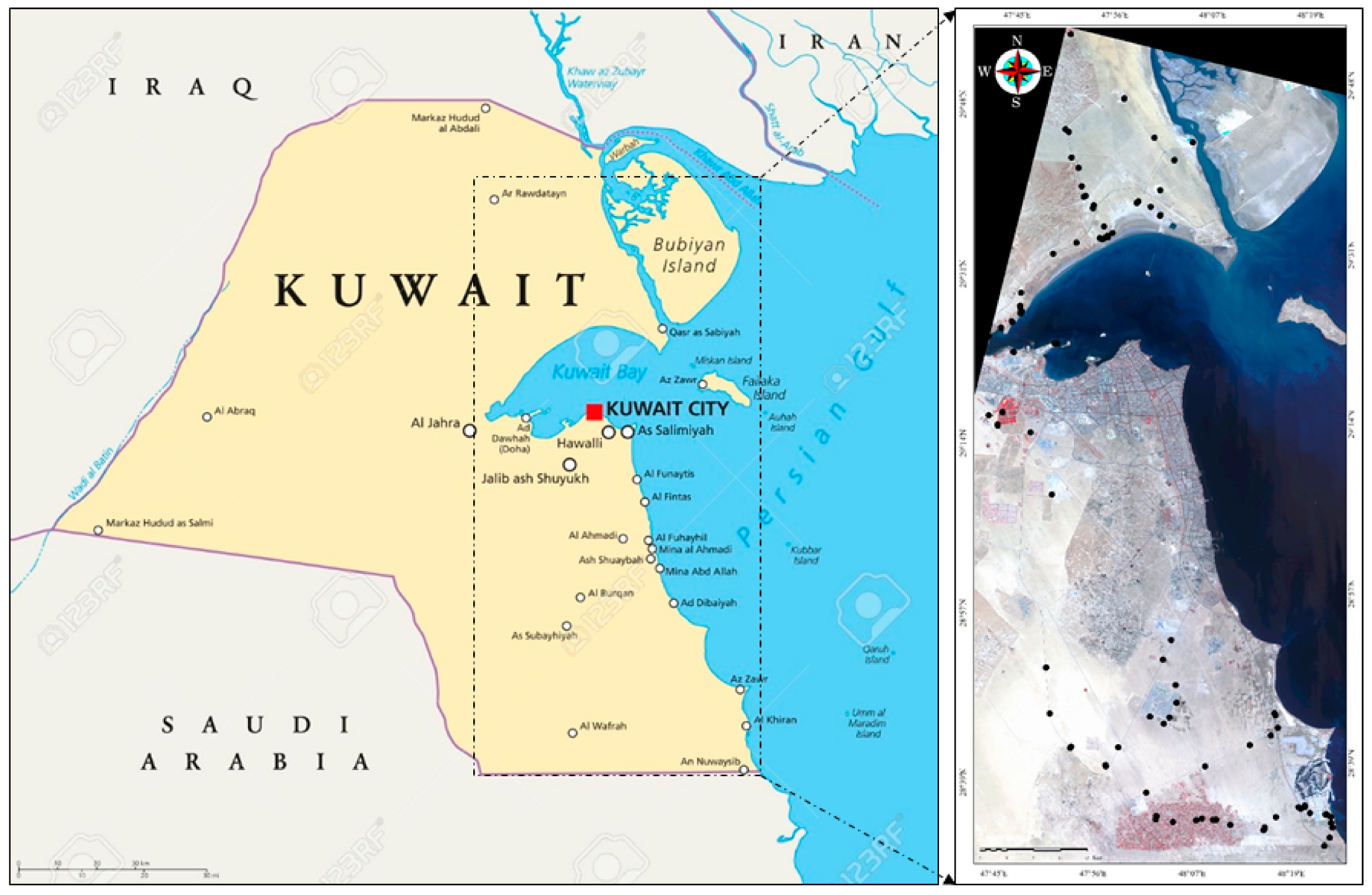
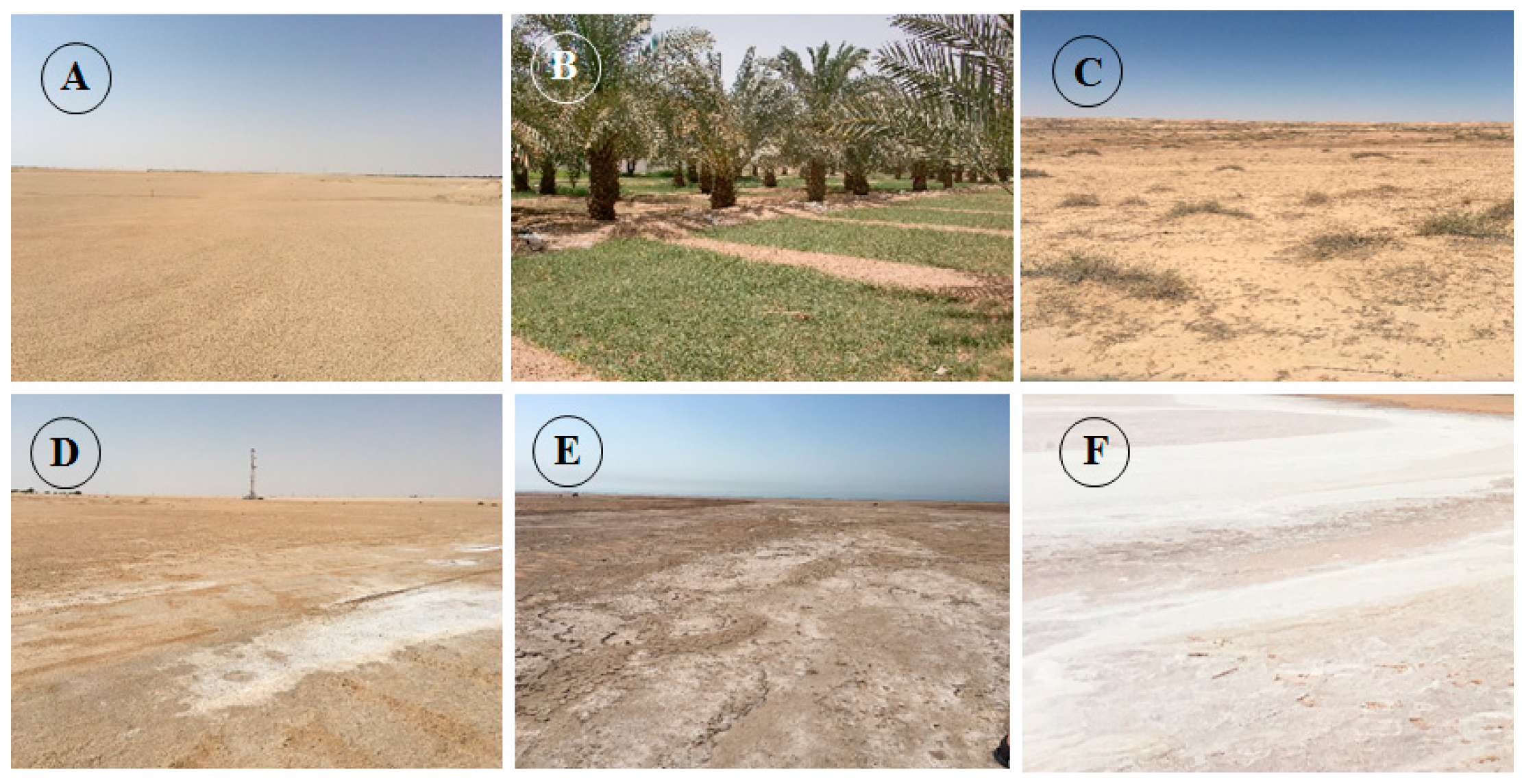
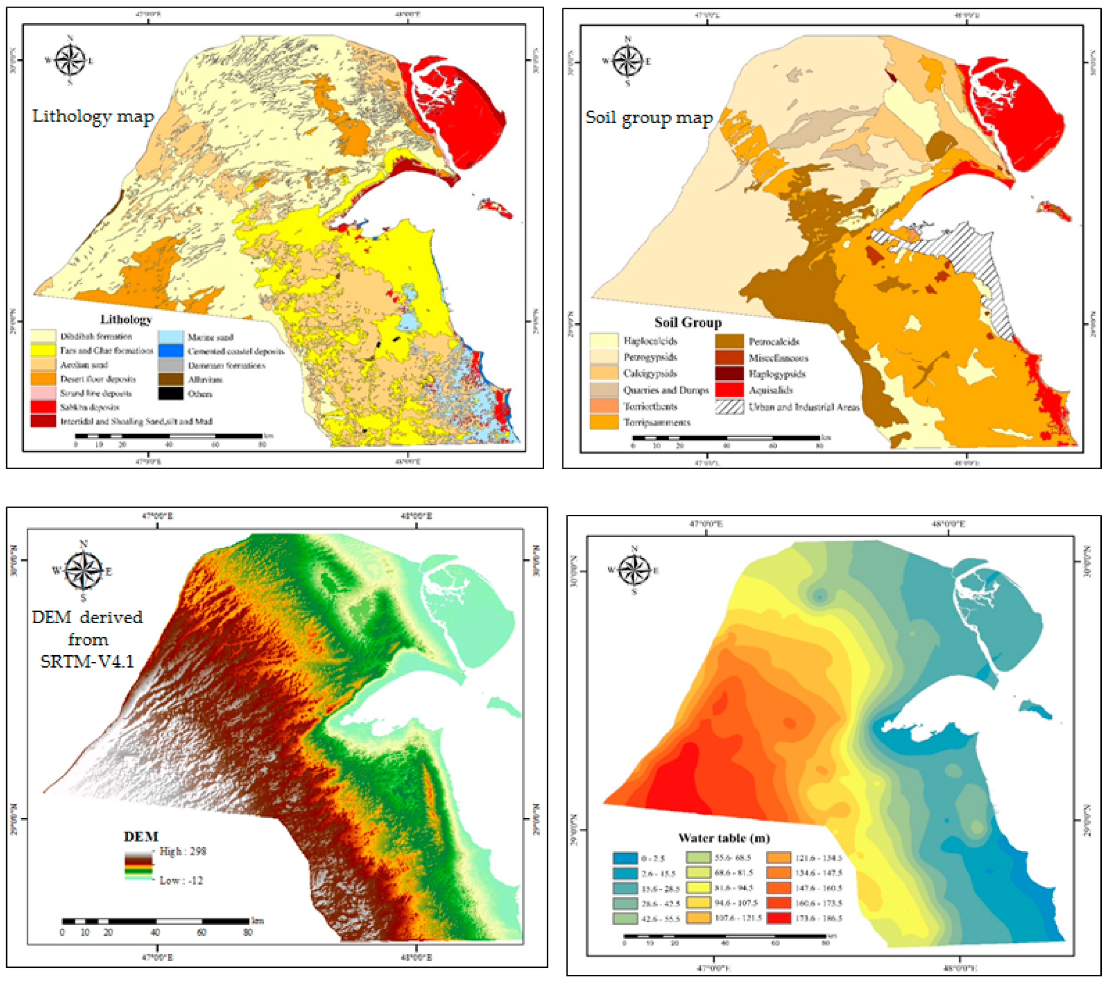
The methodology flowchart involving five fundamental steps is summarized in Figure 1. Firstly, a field survey was conducted over 4 days (15th to 18th May 2017) and a total of 100 soil samples were collected representing different salinity classes, such as non-saline, low, moderate, high, very high and extreme salinity. Then, soil laboratory analysis was accomplished to derive EC_-Lab, pH, the major soluble cations and anions for the used model validation purposes. Secondly, the OLI image acquired on the 13th May 2017, two days prior to the field survey is named “reference scene,” was radiometrically calibrated and atmospherically corrected using the Canadian Modified Simulation of the Satellite Signal in the Solar Spectrum (CAM5S) radiative transfer code [64] integrating the atmospheric variables that interfere during the image acquisition. Subsequently, in the third step, the predetermined SEPM was implemented on this preprocessed “reference scene” to derive the predicted soil salinity map. Statistical analysis (p ˂ 0.05) was applied to find out whether the differences are significant between the predicted salinity (EC_-Predicted) and the measured ground truth (EC_-Lab) for the SEPM validation. In the fourth step, the Landsat serial time’s data (TM, ETM+ and OLI) were radiometrically calibrated, as well as atmospherically and spectrally normalized using the semi-empirical line approach (SELA), which is based on the pseudo-invariant targets [65]. Thereby, soil salinity maps for the three considered decades were derived through the application of the SEPM on the image series. Finally, for the fifth step, the measured and archived climatic variables over the study area between 1970 and 2017 were preprocessed, analyzed and fitted with the quantified soil salinity areas during the study period to track the change trend of the salt-affected soils on spatial and temporal basis.

2.1. Study Area

The state of Kuwait (Figure 2) situated in north western part of the Arabian Peninsula (28°45′ to 30°06′ N, 46°33′ to 48°35′ E) is characterized by arid climate, very hot summers (46.8 °C), irregular and scanty rainfall with an annual mean of 118 mm. The main geomorphological features are Wadis, escarpments, sand dunes, Sabkhas, depressions, playas and alluvial fans [66,67]. These Features are controlled by three types of surface deposits [68]. First, Aeolian deposits such as dunes and sand sheet. Second, evaporates such as halite (NaCl), gypsum (CaSO₄·2H₂O) and anhydrite (CaSO₄) and other salts deposits in coastal and inland Sabkhas. Third, fluvial deposits such as pebbles and gravels along the Wadi Al-Batin channel. Each of these deposits has specific geomorphic characteristics based on their origin, climatic impacts and topography that is generally flat and smooth (gradient of approximately 2 m/km) with a low relief decreasing from southwestern part towards the Arabian/Persian Gulf [67,69]. Geologically, Kuwait stratigraphy consists of two Stratigraphic Groups; Kuwait Group and Hasa Group [70] consisting of six Formations, four of them are exposed in the outcrops represented by Dammam, Ghar, Mutla and Jal-AzZor Formation. Dammam Formation from Hasa Group (Eocene) consists of white fine grained cherty limestone and form some karst. The three other Formations are composed mostly of sandy limestone, calcareous sandstones, sand and clay. Soils of Kuwait are mostly sandy with variable quantities of calcareous materials. Moreover, Gatch layer “hardsetting” occurs in many Kuwaiti soil, which is considered a calcic and/or gypsic pan [71]. Based on the Landsat satellites orbits, more than half of the Kuwait territory (center and east) was used as an experimental area for this study (Figure 2) including irrigated agricultural fields, desert land, urban areas, coastal zones, and low-land such as Bubiyan Island.

2.2. Field Work and Laboratory Analysis

According to the United States Department of Agriculture [72], soils of Kuwait are low in organic matter, mostly sandy and infertile. The soils of Kuwait have been classified into two soil orders; the Aridisols constituting 70.8% and the Entisols forming 22.56%, while the other restricted and marginal groups represent the remaining percentage (6.64%). These two soil orders consist of seven soil great groups based on the morphology, mineralogical, chemical and physical characteristics and miscellaneous area unit [71,72].The extreme salinity class (Sabkhas) is classified in the soil great group “Aquisalid” occurring on the coastal flats and inland Playas containing very high content of salts and gypsum. High salinity class is recognized in the soil great group “Haplocalcid” attributing to a layer of carbonate masses and salt contents. Moderate to low salinity class occurs in “Petrocalcid“ soil, which is well to moderately drained and with calcareous hardpan overlying sandy to loamy soils.

Based on the field work and soil map, the soil salinity is categorized into six classes as illustrated in Figure 3(A) non-saline, (B) low, (C) moderate, (D) high, (E) very high and (F) extreme salinity. As stated above, 100 soil samples representing six salinity classes were collected from the upper 10 cm depth from an area of 50 cm × 50 cm. The samples were placed in sealable plastic bags and properly numbered. Each soil sample was physically described (color, brightness, texture, etc.), photographed and geographically localized using accurate GPS (σ ≤ ±30 cm). The recorded GPS coordinates were connected in real-time to a GIS database integrating the OLI “reference scene” (acquired on 13th May 2017, that is, thereabouts simultaneously with the field survey) to obtain accurate spatial location and identification of each salinity class for validation step (Figure 1).

In the laboratory, the soil samples were air-dried and processed to pass through a 2 mm sieve. The saturated soil paste extract method was used to measure the EC_-Lab and pH. Moreover, the major soluble cations (Ca²⁺, Mg²⁺, Na⁺ and K⁺) and anions (Cl⁻ and SO₄²⁻) were measured using standard procedures and the sodium adsorption ratio (SAR) and exchangeable sodium percentage (ESP) were calculated using standard calculation procedures [31,32]. Because the electrical conductivity of extract from a saturated soil paste is considered an accurate measure of soil salinity, the derived EC_-Lab values for all sampling locations were overlaid on the remote sensing predictive salinity map (EC_-Predicted) in a GIS environment based on GPS locations for spatial correspondences and statistically analyzed between field sampling point values and their homologous pixels for validation.

2.3. Images Data

The Landsat satellite series has acquired medium spatial resolution global imagery continuously since the launch of first Landsat in 1972 [54,55,56,73,74,75] to support research in Earth observation for change detection, environment monitoring and decision making [59,76,77,78,79]. The Landsat satellite series has been used across disciplines to achieve an improved understanding of the Earth’s land surfaces changes and the impact of climate and human activity on the environment. With their seven spectral bands covering the visible and near infrared (VNIR), short weave infrared (SWIR) and thermal infrared (TIR) bands of the electromagnetic spectrum, the three instruments TM, ETM+ and OLI onboard Landsat satellites represent a unique historical record of Earth surface for more than three and half decades. They orbits the Earth similarly onboard Landsat-5, -7 and -8 platforms; collecting data following a sun-synchronous and near-polar orbit at a nominal altitude of 705 km at the equator with a field of view (FOV) of 15° covering a swath of 185 km, an instantaneous field of view (IFOV) of 30-m at the ground and a 16 days’ time repetition at the equator.

The TM is a second-generation sensor in the Landsat program, carried onboard Landsat-4 (1982–1993) and Landsat-5 (1984–2013). It is a whiskbroom instrument imaging radiometer employing oscillating mirror to scan detector fields of view cross-track to achieve the total instrument fields of view [80]. Launched onboard Landsat-7 in 15th April 1999, ETM+ is also a whiskbroom scanning radiometer designed to collect data in the same electromagnetic spectrum and the same radiometric resolution as TM but the specific spectral response profiles differ slightly in all of the solar-reflective bands, nevertheless they are often considered equivalent as illustrated in Figure 4 [81]. On 11th February 2013, the Landsat-8 was launched, transporting two instruments—OLI and thermal infrared sensor (TIRS)—which use long linear arrays of detectors aligned across the instrument focal planes to collect imagery. The OLI is a push-broom sensor with approximately 70,000 detectors, which is a fundamental improvement compared to the earlier Landsat TM and ETM+ which contained significantly fewer (≤136) detectors [82,83]. Likewise to TM and ETM+, the OLI sensor collects land-surface reflectivity in the VNIR and SWIR wavelengths. However, the spectral response profiles of OLI (especially in NIR and SWIR-1 bands) are notably narrower than the corresponding TM and ETM+ bands to avoid atmospheric absorption features (Figure 4) [84]. Moreover, the OLI design results in a more sensitive instrument with a significant amelioration of the signal-to-noise ratio (SNR) radiometric performance quantized over a 12-bit dynamic range (Level 1 data) and raw data are delivered in 16 bit, which is 16 times greater than the eight-bit data performances from TM and ETM+ [85]. The SNR specification is 6 to 10 times better than that of TM and ETM+ for all bands, as well as a set of sophisticated onboard calibration systems to monitor the radiometric stability of the instrument [83,86]. Thus, allowing a superior dynamic range, a reduction of saturation problems and, consequently, enabling better characterization of land-cover signal conditions [87].

Since 2008, the provision of reliable and free Landsat data has attracted great interest from the international scientific community for more widespread use to characterize multi-temporally several natural resources and environmental applications [55]. In this study, a total of ten scenes were used as summarized in

Table 1. Landsat images used in the present study.

Satellite	Sensor	Acquisition Date	Acquisition Time
Landsat-5	TM	14/07/1987	09:41:25
Landsat-5	TM	28/08/1992	09:38:38
Landsat-5	TM	29/08/1998	09:54:54
Landsat-7	ETM+	11/09/2000	10:06:57
Landsat-7	ETM+	17/09/2002	10:04:03
Landsat-7	ETM+	20/03/2006	10:06:22
Landsat-7	ETM+	03/12/2009	10:06:24
Landsat-8	OLI	05/07/2013	10:18:15
Landsat-8	OLI	14/08/2016	10:16:19
Landsat-8	OLI	13/05/2017	10:15:41

—three TM, four ETM+ and three OLI scenes. These selected images are not cloudy, not contaminated by cirrus and without shadow effects because significant topographic variations are absent in the study area. The geometric registration precision among these images is better than 0.15 pixels and no visual obvious miss-registration was observed when they were overlaid for analysis.

2.4. Images Data Preprocessing

Prior to launch, the sensors are subject to rigorous radiometric and spectral characterization and calibration in the laboratory using integrating sphere. However, post-launch absolute calibration is an important step to establish the relationship between at-sensor radiance and the digital number output for each pixel in the different spectral bands. Sensor drift radiometric calibration, sun illumination geometry and atmospheric corrections (scattering and absorption) are fundamental preprocessing operations to restore the images radiometric quality at the ground level for monitoring inter-annual or even seasonal vegetation cover and soil conditions [88,89]. The capability to detect and to quantify changes accurately in the Earth’s environment depends on the quality of these preprocessing steps. In fact, the correctness of interpretation and information extraction from a long-term series of remote sensing products requires accurate discrimination between scene artifacts and changes in the Earth surface processes being monitored [76,90]. The changes caused by these artifacts can be mistakenly attributed to changes in the land use and ground bio-physiological components and errors can propagate in all subsequent image processing steps, such as spectral indices calculations, multi-temporal analysis, climate change impact investigation and modeling and so forth [81,88,91,92,93,94,95]. The preprocessing tasks in this study were achieved in two inter-related steps. The first deals with rigorous physical corrections of OLI-2017 image acquired almost simultaneously with the field survey. Based on the results (ground reflectance’s) of the first step that was used as a “reference scene,” the second step involves a cross-calibration procedure based on SELA and pseudo-invariant targets [65] for atmospheric and spectral normalization [96,97,98].

2.4.1. OLI Reference Scene Preprocessing

Acquired at the top of the atmosphere (TOA), the raw OLI-2017 scene was transformed into apparent equivalent radiance using appropriate radiometric absolute calibration parameters delivered by EROS-USGS center for each spectral band. Then, the extra-atmospheric irradiance, the solar zenith angle and the Earth-sun distance (in astronomical units) were used to transform the apparent radiance to the apparent reflectance at the TOA. Moreover, the CAM5S model [64] based on Herman radiative transfer code was used for atmospheric conditions simulations to calculate all the requested atmospheric correction parameters in each spectral band of OLI-2017 image (reference scene). The CAM5S model simulates the signal measured at the TOA from the Earth’s surface reflecting solar and sky irradiance at sea level, while considering the sensor characteristics, such as the band passes of the solar-reflective bands (Figure 4), satellite altitude, measured atmospheric conditions during the satellite overpass, atmospheric model, sun and sensor geometries and terrain elevation. Consequently, all the requested atmospheric correction parameters were used to transform the apparent reflectance to the ground reflectance. Sensor calibration and atmospheric interferences were then combined and corrected in one-step using PCI-Geomatica [99] to preserve the radiometric integrity of the image data [100].

2.4.2. Multi-Sensors Data Inter-Calibration

The used historical Landsat data recorded by TM, ETM+ and OLI sensors must be inter-calibrated to derive temporally consistent soil spectral signatures, allowing soil salinity to be estimated using a single and consistent model [38]. Similarly to the first step, all the considered scenes were transformed to the apparent reflectance’s using the “gain” and the “offset,” the extra-atmospheric irradiance, the solar zenith angle and the Earth-sun distance. At this step, all the considered scenes were rescaled to eight-bit radiometric resolution.

Furthermore, the atmospheric effects contribute significantly to the signal received by optical remote sensing satellite systems and a serious problem arises when the measurements of the atmospheric parameters are absent. To remedy this situation, many methods were developed and reported in the literature to remove or at least to normalize these impacts from images acquired in different times with a series of satellite sensors [101]. The SELA based on pseudo-invariant targets was proposed by Morin et al. [65] to link the apparent reflectance to the ground reflectance (illumination, atmosphere, spectral and response profiles normalization). These targets must be significantly stable in time, large enough, near Lambertian, uniform soil color across the target, absence of vegetation and low variance in reflectance through time [89,102]. This approach has been used in various radiometric cross-calibration studies involving data acquired with different sensors in different times [98,103]. According to Morin et al. [65], to take account of atmospheric path radiance, it is necessary to have at least two spectrally different targets within the scene to develop SELA equations, bright and dark targets with, respectively, high and low reflectances. However, the use of more than two targets allows greater confidence between at sensor apparent reflectances and ground surface reflectances correction equations [96,97]. Based on three pseudo-invariant targets such as asphalt, bright and dark sandy soils; this method was applied in this study to remove atmospheric effects and to normalize the spectral and response profiles difference among the considered scenes acquired with TM, ETM+ and OLI sensors.

2.5. Image Data Processing

In addition to the remote sensing sensors technology improvement and innovation, several image processing methods and models were developed and applied for soil salinity retrieval including spectral salinity indices [50,104,105,106,107], mixture-tuned matched filter approach [108], regression of multi-spectral bands [109,110,111], partial least square regression [39,105], multivariate adaptive regression splines [112], artificial neural network model [113], linear spectral mixture analysis [114], machine learning regression [115] and several empirical and semi-empirical predictive models [40,41,42,43,44,106,107,116,117]. These last models were developed for different geographic regions around the world, that is, Latino-America (Mexico), Middle-East (Iraq), north and east Africa (Morocco and Ethiopia) and Asia (China) [44]. Moreover, they integrated different spectral bands and unlike mathematical functions in their conceptualization (stepwise, linear, second order, logarithmic and exponential functions) based on simulated spectral data and/or satellite images acquired with different sensors such as TM, ETM+, OLI, Sentinel-MSI, EO-1-ALI, Worldview-2 and WorldView-3 [41,42,104].

Furthermore, for soil salinity mapping, several studies revealed that spectral confusion occurs in the VNIR spectral domain between the salt crust and the artefacts of soil optical properties [41,42,43,118,119,120,121,122,123]. In these wavelengths, the main factors affecting the salt-affected soil spectral signatures are represented by the salt types, the soil mineralogy, level of moisture, organic matter content, soil color and brightness, roughness and vegetation cover [124]. Obviously, these factors influence the signal gathered by the sensor in a specific pixel area causing severe confusions between the salts in the soils and the soil optical properties [120,121]. The continuum removed reflectance spectrum and the first derivative investigation, as well as statistical fit between individual spectral bands and EC_-Lab revealed that only the SWIR bands were correlated significantly (R² > 50%); while the R² between the VNIR bands and EC_-Lab remains less than 9% [43]. In addition, as documented in the literature during the last two decade, the SWIR spectral domains allows better discrimination among soil salinity classes and were integrated in soil salinity modeling and monitoring at local, regional and global scales [125]. Indeed, Shrestha [126] showed that the SWIR bands are the most correlated with soil salinity. Bannari et al. [41,42,104] found that the SWIR bands of ALI EO-1, OLI, Sentinel-SMI and WorldView-3 offer the best potential for soil salinity detection and discrimination. Considering different soil types at several geographic locations, Leone et al. [127], Odeh and Onus [128] and Zhang et al. [106] demonstrated that the SWIR bands could be used for soil salinity estimation in agricultural fields better than VNIR spectral domains. Chapman et al. [129] indicated that the SWIR bands of TM provide excellent discrimination of evaporite mineral zones in salt flats. Drake [130] described the various absorption peaks of the salts found in evaporite minerals in the SWIR wavelengths. The study undertaken by Hawari [131] showed that the absorption features in SWIR bands are consistent with the detection of the gypsum, halite, calcium carbonate and sodium bicarbonate. According to Nawar et al. [112], the SWIR bands of Advanced Space-borne Thermal Emission Reflection (ASTER) exhibited the highest contribution for soil salinity discrimination. Moreover, Rahmati and Hamzehpour [132] indicated that the SWIR bands of the ETM+ sensor increases the accuracy of the soil salinity prediction.

Comparative studies among several empirical and semi-empirical predictive models were completed for accurate soil salinity characterization and detection. Bannari et al. [40] compared them on irrigated agricultural land in North Africa where only slight and moderate salinity classes are present, while El-Battay et al. [63], Bannari et al. [41] and Alali et al. [44] tested them on arid landscape (Middle-East) considering a wide range of salinity classes from slight to extreme. These studies showed that the SEPM model based on the Soil Salinity and Sodicity Index (SSSI) integrating the SWIR bands provided the best accuracy for soil salinity classes’ discrimination and mapping, therefore it was considered in the present study. It was implemented, calculated and validated using ground truth and the OLI “reference image” acquired during the 13th May 2017 and then applied to all other considered images. The equation of this SEPM is the following [40]:

EC_-Predicted = C^st·[4521·(SSSI)² + 125·(SSSI) + 0.41]

(1)

SSSI = (ρ_SWIR-1·ρ_SWIR-2 − ρ_SWIR-2·ρ_SWIR-2)/(ρ_SWIR-1)

(2)

where:

• EC_-Predicted: Predicted electrical conductivity semi-empirical model,
• C^st: Scaling factor,
• ρ_SWIR-1: Reflectance in MSI and OLI SWIR-1 channel, and
• ρ_SWIR-2: Reflectance in MSI and OLI SWIR-2 channel.

C^st theoretically enables an up-scaling between the spatial information measured in the field and its homologous information derived from the image. Several methods were applied to calculate this factor depending on the remote sensing applications [133]. In the present study, a simple up-scaling empirical ratio was calculated between the observed and the predicted values considering six sampled points representing the six salinity classes (extreme, very high, high, moderate, low and non-saline). Homogeneous and uniform pixel surface representing each class was located using the GPS coordinates. The homologous ground reference values resulting from the laboratory analysis (EC_-Lab) were used to calculate an average and global scaling factor for the entire image.

2.6. Climatic Data

During the last half century, automatic climate and weather forecast station networks were established in Kuwait. Currently, the meteorological network is composed of 28 stations geographically distributed to cover the regions located within the territorial borders of the country forming the most spatially and temporally complete record of climatic variables in Middle-East. Definitely, the availability of the collected data by these stations over a very long-time period makes them relevant and useful within the context of climate change impacts analysis over this region. The digital archives of temperatures and precipitations on daily basis (hourly weather observations) recorded between 1970 and 2017 were averaged on monthly and yearly basis and then used as input for analysis.

2.7. Statistical Analysis and Model Validation

Remote sensing of soil salinity mapping is intrinsically associated with uncertainties, therefore, a well-designed validation method is required. In the present study, statistical analyses were computed using “Statistica” software. Various statistical parameters were calculated for both EC_-Lab obtained from the laboratory analysis and the EC_-Predicted values derived from OLI “reference scene” using the SEPM. Standard deviation was indicated in all cases as an error percentage of the average values of EC_-Lab and EC_-Predicted. For validation purposes, EC_-Lab and EC_-Predicted were compared using the 1:1 line. Ideally, observed and predicted values should have a correspondence of 1:1. The index of agreement (D) reflects the degree to which the observed value is accurately estimated by the predicted value. This measure was calculated as follows [134]:

$$D=1-\left[\frac{{\displaystyle \sum _{i=1}^n{\left(P_i-O_i\right)}^2}}{{\displaystyle \sum _{i=1}^n{\left(\left|P_i^{\prime }\right|+\left|O_i^{\prime }\right|\right)}^2}}\right]$$

(3)

where P_i is the predicted value at sample I; O_i is the observed value at sample I; P_i′ is the difference between P_i and the average of the predicted values; O_i′ is the difference between O_i and the average of the observed values and n is the number of values. This index provides a measure of the degree to which a model’s predictions are error-free. It ranges between 0 and 1, with 1 indicating a perfect match between observed and predicted values. The root mean square error (RMSE) was used as an overall error to supplement the index of agreement described above. This error also quantifies the 1:1 relationship between observed and predicted values. It was calculated as follows [134]:

$$RMSE=\sqrt{\frac{{{\displaystyle \sum }}_{i=1}^n{(P_i-O_i)}^2}{n}}$$

(4)

The relationships between EC_-Lab and EC_-Predicted were also analyzed using a linear regression model (p ˂ 0.05) and the R² was used to evaluate the strength of the regression curve of the linear relationship. Systematic linear over-predictions or under-predictions generate characteristic variations in the slope and intercept values, which can help to interpret the major sources of error and the potential of the SEPM for salinity mapping and prediction using OLI “reference scene”.

3. Results Analysis and Discussion

3.1. Salinity Model Validation: Visual and Statistical Analysis

To understand whether the applied SEPM is relevant and reliable to predict accurately soil salinity classes in this arid landscape, a validation procedure was conducted to examine its ability to predicted results against the ground truth. To achieve this step, the derived soil salinity map analysis and validation were undertaken visually by reference to the field observations and ancillary data (soil, lithology, topography and water table maps) (Figure 5) and statistically based on the EC_-Lab. In the PCI-Geomatica image processing system, water surfaces of the Arabian/Persian Gulf were masked and the histogram of the derived salinity map from OLI “reference scene” was thresholded based on the defined six major salinity classes (Figure 6) including non-saline (class 1 in blue), low (class 2 in cyan or sky-blue-green), moderate (class 3 in clear green), high (class 4 in yellow), very high (class 5 in orange-red) and extreme salinity (class 6 red-purple). Indeed, the values of the centroids of clusters representing these six major classes were considered; as well as, the value of the standard deviation was chosen to limit the overlap between the classes considered and to reduce the chance of a pixel being classified into more than one class.

Table 2. Thresholding values and EC_-Lab limits for the considered soil salinity classes.

Class Number	Class Name	Thresholding Values	EC-Lab Limits (dS/m−1)
1	Non-Saline	0–10	0–4
2	Low salinity	11–25	4.5–10
3	Moderate	26–51	10.5–20
4	High salinity	52–102	20.5–40
5	Very high salinity	103–152	40.5–60
6	Extreme salinity	>152	≥61

summarize the thresholding values and the EC_-Lab limits for each soil salinity class. Over the study area, these classes occupied 51.4%, 30%, 12.9%, 2.9%, 1.4% and 1.4% for non-saline, extreme, low, moderate, high and very high salinity, respectively. Visual analysis reveals an excellent conformity of this map with the ground truth. For instance, the extreme salinity class is pure salt, marine sand and cemented coastal deposits forming a Sabkha, which occur in the Aquisalids soils. As shown in Figure 6, this class is located in all areas along the coastal zones of Kuwait Bay, in lowlands and Bubiyan Island, in playas and in coastal flat zones above the high tide level with very low topography (<1.2 m) and the water table is very near to the surface remaining within 1.00 m. These sabkha zones create a chemically aggressive environment and lead to a structurally unstable soil condition with high contents of soluble salts and the surface salt crust. They are natural uncultivated land (loamy and sandy, highly gypsiferous) and devoid of any vegetation. According to the laboratory analyses, sulfates, chlorides and carbonates of sodium, calcium and magnesium dominate the salt content in this sabkha soil. Seawater intrusion and subsequent evaporation results in surface crusts, especially in these zones of capillary rise where the slope is near to zero, thus facilitating water catchment and retention. This situation generally occurs in a dry climate, such as the case of Middle Eastern countries, where the total annual precipitation is very low (~100 mm/year), the temperature is very high most of the year accelerating the evapotranspiration and the salt accumulation at the soil surface.

The very high and high salinity classes are also located in the coastal zones but with a relatively low slopes, in Bubiyan Island, as well as in some inland areas. These classes are linked to Aquisalids soils which are sandy to clayey with a layer of gypsum crystals, poorly drained with a layer of salt accumulation near the surface and water table remains within the upper 1.0 m. The very high salinity class presents other crustal features including a bare level soil surface, often encrusted with an efflorescence of salt crystals and a well-developed platy structure, which looks like the creation of a new sabkha. The high salinity class is composed of fine, white, sand-sized shell gravel and gravelly sand in which the surface layers are sometimes cemented by salt. The texture of this area is a mixture of medium and fine sand-grade quartz with moderate amounts of carbonates. The soil surface (~5 cm) becomes cemented, forming a strong white-brown salt-crust. In other places, the immediate top surface becomes indurated into a brittle crust, which is ridged into many undulations with an amplitude of 3 to 5 cm. Moreover, the areas of high and very high salinity classes are also completely devoid of vegetation.

The moderate salinity class located in the northwest and southwest (border with Saudi-Arabia) associated with sites of oil industry infrastructure and field operations. In these locations the water table is at a depth greater than 80 m and the terrain elevations are higher than 150 m. This class is also located in the highest areas of Bubiyan Island and is composed of two soil great groups, the Petrocalcids (sandy to loamy soil overlying a calcareous hardpan) and Haplocalcids (sandy to loamy soils with a layer of calcium carbonate crystals in soil matrix). The petrocalcids soils are not suitable for agricultural production. However, very sparse and scattered clumps of halophytic plants are observed in this class area. According to the field visit, laboratory analyses and ancillary data, we found that these four saline classes (extreme, very high, high and moderate) are often rich in sodium chloride, calcium sulfate and associated with shales and marls, limestone and dolomitic-limestone. Their gypso-saline characteristics cause the formation of salt strata that are thrust upward to the surface from the underlying salt bed. These saline formations are often associated with anhydrite, gypsum, sulfur and paleo-lagoonary sedimentary rocks.

Low salinity class is located in the agricultural lands in the north (Abdali region) and south (Al-Wafra region) of the study area. This class includes the only cultivated areas in Kuwait (1% of the total area of the country), which are totally equipped with modern irrigation systems and mainly used for growing date palms, alfalfa, vegetables and fodder crops. This class is dominated by two soil great groups (Torripsamments and Haplocalcids), located in flat areas with a low altitude (~20 m) and a water table below 15 m. The Torripsamments is a native soil in Kuwait generally non-saline with low fertility potential, classified as a sandy or loamy sandy while the Haplocalcids is a sandy to loamy soil with masses of calcium carbonate in the soil profile. These soils are moderately suitable for irrigated agriculture. However, due to the salinity of irrigation water some patterns in this region are showing a very high salinity level. Finally, the non-saline class is composed of two main soil groups (Torripsamments and Petrogypsids), that is, sandy to loamy soils overlying a gypsic hardpan or a gypsic horizon underlain by a calcic hardpan with relatively high topography (≥50 m) and a moderately deeper water table (>30 m). This accurate visual interpretation and discrimination analyses among different salinity classes demonstrates the robustness of the applied SEPM and its high sensitivity to the complexity of salinity classes in this arid landscape.

Furthermore, the major cations (Ca²⁺, Mg²⁺, Na⁺ and K⁺) and anions (Cl⁻ and SO₄²⁻), pH, EC_-Lab and SAR values were determined in the laboratory from saturated soil paste extract.

Table 3. Chemical properties of different soil salinity classes.

Salinity Classes	Average EC-Lab	pH	Ca2+	K+	Mg2+	Na+	Cl−	HCO3	SAR
	dS/m−1		meq/L						(mmoles/L)0.5
Non-Saline	2.6	7.6	39	1.8	7.8	32	9.6	6.6	3.4
Low	6.7	7.7	67	2.3	12	23	38	9.1	3.5
Moderate	11.8	7.7	45	7	14	49	70	10	9.1
High	38.4	7.3	146	310	100	258	350	6	23.3
Very high	48.8	7.4	78	15	19	325	590	4	46.8
Extreme	300	7.0	230.5	97	1118	3615	3932	6.6	166.5

summarizes the six classes of salinity according to the EC_-Lab values and present the mean values of cations and anions in each class. According to these analyses, the soil samples are in general highly affected by chloride (Cl⁻) and sodium (Na⁺), magnesium (Mg²⁺) and calcium (Ca²⁺) than other elements. Besides, the EC_-Lab and SAR are increased gradually and very largely from non-saline (EC_-Lab = 2.6 dS/m⁻¹, SAR = 3.4) to extreme salinity in Sabkha (300 dS/m⁻¹ ≤ EC_-Lab, SAR ≤ 166.5). Obviously, these results are in agreement with the predicted salinity classes ascertained by remote sensing image processing as discussed above. Sequentially, the soil pH values in the range from 7 to 7.7 indicated slightly alkaline reaction due to the preponderance of bicarbonate (HCO⁻₃) in the soils with a range from 4 to 10 meq⁻¹.

Figure 7 illustrates the relationship between EC_-Lab and EC_-Predicted derived from the applied SEPM. This statistical validation procedure highlights the potential of this model integrating the SWIR bands, which is sensitive to soil-salt mineralogy, providing a regression fitness with a good D of 0.84, an excellent R² of 0.97 and low RMSE of 0.13 at significance level of p ˂ 0.05. The scatter-plot reveals a good linear relationship between the EC_-Lab and EC_-Predicted in term of good fit 1:1 showing an excellent spatial variability of salinity (1.3 ≤ EC_-Lab ≤ 400 dS/m⁻¹). In spite of this model was developed for slight and moderate salinity in semi-arid irrigated agricultural land [40], the present study showed an appropriate prediction for the different salinity classes investigated in arid landscape. However, slight overestimation is observed for high salinity class with the EC_-Lab range from 50 to 170 dS/m⁻¹, as well as less underestimation caused by saturation was pointed out for the very high and extreme salinity classes (EC_-Lab ≥ 400 dS/m⁻¹) resulting in the points not fitting the 1:1 line very well. The slope (0.91) and the intercept (7.76) corroborate these observations by expressing a slight deviation from the 1:1 line (Figure 7). Indeed, this underestimation is probably attributed to the impact of soil moisture in Sabkha and shorelines (very high and extreme salinity classes) on the signal recorded by the SWIR bands that are sensitive to soil humidity. Moreover, this is probably due to the saturation of the signal gathered at the satellite level for pixels of very high and extreme salinity classes. The slight overestimation could be due to the scale factor that was estimated between field samples identified from an area about 50 cm × 50 cm and its homologous points in the OLI “reference scene” represented by 900 m² pixel size. In addition, the preprocessing steps of OLI data are essential for the removal of sensor artifacts and atmospheric interference effects. It is also probable that the residual errors persist due to uniform correction of each spectral band and not pixel-by-pixel, which has caused a small difference between the EC_-Lab and the homologous EC_-Predicted calculated from remote sensing image. Eventually, despite these small variations, the validation of this applied model provides satisfactory results when compared to the ground truth data, indicating that this model is appropriate and extendable to other images acquired multi-temporally. These results corroborate findings of relevant studies over irrigated agricultural lands in semi-arid as well as in arid environments [40,41,63].

3.2. Landsat Series Datasets Inter-Calibration

The OLI “reference scene” almost thereabouts simultaneously with the field survey was transformed rigorously to the ground reflectances using the CAM5S as a physical atmospheric radiative transfer code, the measured atmospheric parameters during the satellite overpass and the sensor radiometric-drift calibration parameters. This step was achieved with an accuracy better than ±3% as reported by Markham et al. [135], Li et al. [136] and Gascon et al. [137]. This “reference scene” ground reflectances was used for Landsat series data inter-calibration. The 10 used scenes have been geometrically projected using Universal Transformed Mercator (UTM) coordinate system and World Geodetic System 1984 (WGS84). Since the Landsat data used were collected under favorable meteorological conditions that has reduced the uncertainties. Likewise, the multi-temporal atmospheric corrections and spectral normalization method based on SELA was implemented and applied using three pseudo-invariant targets such as asphalt, bright and dark sandy soils. To establish a linear regression by relating the spectral bands of the “reference scene” to their homologous bands in the other considered images, 60 pixels were extracted from each image by selecting twenty sample pixels from each target (asphalt, bright and dark sandy soils). The results exhibited the SELA produced very accurate inter-calibration of Landsat TM, ETM+ and OLI image datasets in arid landscape for the 30 years investigated [97]. Indeed, with respect to the “reference scene,” the established inter-calibration equations regarding SWIR bands that are integrated in SEPM were achieved with an excellent curve fitness (R² ≥ 0.92) for the considered scenes acquired with the three sensors. Accordingly, the RMSE of the ground reflectances were retrieved with accuracies less than ±5% for TM and ETM+. This order of magnitude of the RMSE concurred with the expected absolute radiometric calibration accuracy for archival data acquired with these both sensors, as reported by Chander and Markham [138]. Thereby, according to Thome [139] and Thome et al. [140] the absolute uncertainties of the reflectance-based method for these sensors is in the ±3% to ±5% range, which fits well our inter-calibration results, while the achieved RMSE for OLI data acquired in 2013 and 2016 varies between ±1% and ±5%, which corroborates the finding of Markham et al. [135]. Definitely, these accuracies (±1% to ±5%) remained suitable and fitted well to the calibration standards of the three considered sensors (OLI, TM and ETM+). Moreover, independently to the selected targets for SELA (bright and dark sandy soils or asphalt) and the sensors characteristics, an excellent consistency was observed between the ground reflectances in all homologous spectral bands of the considered 10 images sequence. These results demonstrate the potential and utility of SELA in arid environment for multi-temporal studies using Landsat remote sensing satellite systems, providing corrected images with good quality-assurance to retrieve biophysical and/or geophysical parameters comparable in time [97].

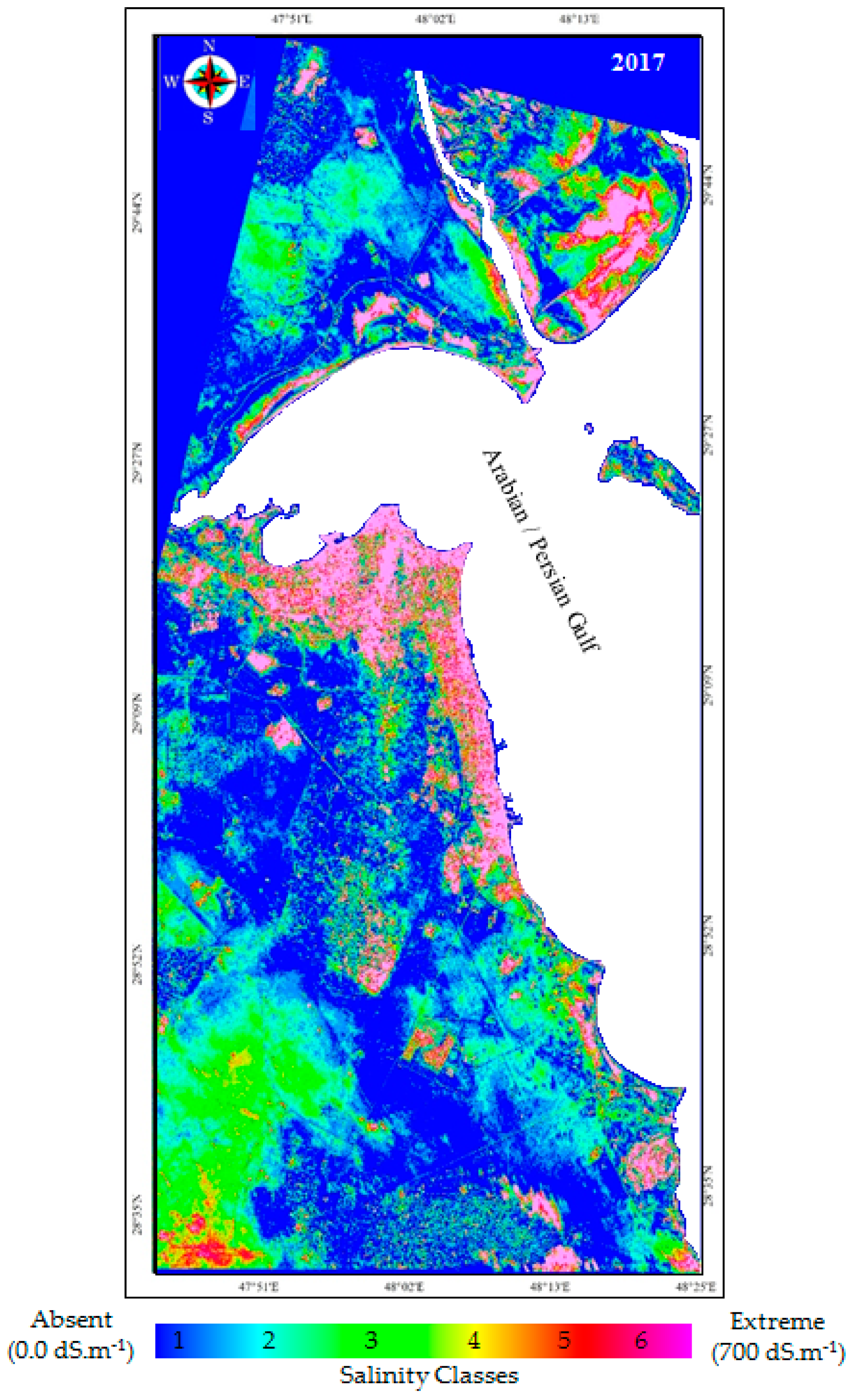
3.3. Spatiotemporal Salinity Maps and Change Trend Analysis

Figure 8 illustrates the derived multi-temporal salinity maps over the study area between 1987 and 2017 using the SEPM (maps unit in dS/m⁻¹ and Table 2 summarize the EC_-Lab limits for each salinity class). Comparison of salinity maps exhibits strong changes and increase of soil salinity, especially in areas along the coastal zones of Kuwait Bay and also extended to non-coastal areas. These maps provide the historical spatiotemporal soil salinity dynamics during the last three decades in the study area of Kuwait. Although, due to the lack of a historical database of salinity measurements for validation, it was not possible to determine the validation targets but the maps produced in the present study are considered reliable for monitoring and quantifying changes in each considered soil salinity class, this is due to the fact that the used model was recently validated for 2017 as discussed above.

The derived reference map for 1987, covering a total salted area of 433 km², shows that the non-saline and low salinity classes are dominant. Whereas, the moderate and very high salinity classes are relatively less present and located only in the coastal zones and the lowlands of Bubiyan Island where the groundwater table is very near to the surface (<1.00 m) exacerbating the salt accumulation in the soil through capillary movement and subsequent evaporation. In these regions, the soil salinization process over time is the result of sea water intrusion coupled with high temperatures to speed-up the evapotranspiration process. For the reference year 1987, the average of recorded precipitations was 75 mm, while the documented temperatures were 40 °C and 50.6 °C for the average and the maximum, respectively. Unfortunately, these received precipitations are inadequate to accomplish leaching of salts accumulated or originally present in the soil. Normally when the precipitations are around or more than 1000 mm/year the leaching process must take place and the salinity should not be developed [141]. Regrettably, this is not the case in these arid zones, thus favoring salts accumulation in soils.

The 1992 map does not show a spatial distribution of soil salinity patterns similarly to that of 1987. During these five years, non-saline class was declined approximately by 10% while moderate and extreme salinity classes increased by 146% and 130%, respectively. In general, the salt-affected areas increased to 1850 km², equivalent to 350% compared to the area estimated in map of 1987. This drastic dynamic change is the consequence of a very drought period between 1987 and 1991, as well as of the Gulf war in 1991. Indeed, the region first had experienced a very severe drought period recording very low precipitations of 75, 70, 68, 40 and 13 mm during the years 1987, 1988, 1989, 1990 and 1991, respectively. Moreover, during the five years period, temperatures found to be varied between 38 °C and 51 °C for the average and maximum, respectively. Second, as Iraqi forces withdrew from Kuwait during the Gulf war, they set fire to over 790 oil wells and damaged almost 75 more as illustrated by Landsat-TM image and field photos shown in Figure 9 [142]. The Landsat-TM captured the devastating environmental consequences of this war [143], which affected approximately 25% of Kuwait’s soils [144]. In this environmental disaster, fires burned for 10 months and firefighting crews from 10 countries used familiar and also never-before-tested technologies to put out the fires (Figure 9A and (Figure 9B). The flows of crude oil and seawater used to extinguish the burning oil wells were accumulated in these areas. Obviously, excessive temperature of the desert causing high evaporation and leaving behind a mixture of crusts of salt and crude oil burned (Figure 9C and (Figure 9D), caused damages to the natural environment of the desert especially the soil [144,145]. These conditions are considered to be the reasons why the salinity increased extremely in the Bubiyan Island and in the center of Kuwait where the oil wells were destroyed and explain the causes of higher salinity in the north and south, moderate to high in the center-east of the study area and generally moderate along the coastal zones of Kuwait Bay. The comparison of derived salinity maps from the prewar image (1987) and the postwar image acquired in 1992 (nine months after the last fires were put out) demonstrates the nature and the extent of surface change with gradual shift from no soil salinity to moderate and high soil salinity. Certainly, in addition to soil salinity accumulation, these changes are producing alterations to the surface sediment and morphological features that lead to soil salinization, biodiversity loss and environmental degradation.

Six years after the Gulf war, salinity was decreased within an area of 1380 km² during 1992–1998. A substantial reduction is observed in the center and north-west of the study area where the oil wells were burned. These areas are characterized by a lack of vegetation or agricultural fields, far from coastal zones, with a relatively high topographic elevation (~200 m) and the water table is moderately deeper (~40 to 55 m), thus only slight and moderate soil salinity classes are observed. On the other hand, in the south of the study area where agricultural fields begin to develop and the crops are irrigated with brackish water and treated sewage effluent, the salinization process is observed. The extreme salinity class is located only in Bubiyan Island, which is flat lowland where water table exists within the upper 1 meter from the soil surface. During the period 1992–1998, climatic variables showed unsystematic variation pattern (Figure 10). For instance, precipitations were varied between 106 and 215 mm, which relatively favors the leaching process in soils and the reduction of salt accumulation, while the maximum temperatures increased from 48.2 to 51.3 °C. Two years later, in 2000, the temperatures trend remained constant (51 °C), whereas precipitations were declined from 112 to 80.8 mm per annum. Thus, promoting the accumulation of salts, which increased by 720 km² during 1998–2000. In fact, the derived soil salinity map for 2000 (Figure 8) covers a total area of 2100 km². The results revealed that the high, very high and extreme soil salinity classes cover approximately 1050 km² while, the slight and moderate salinization had extended forming a corridor in the NW-SE direction and covering another 1050 km² in the center-west and south-east of the study area. In these inland areas, far from the sabkhats and the coastal zones, the topography is relatively high (~200 m), the water table is deep (~80 to 100 m) and agricultural lands are absent, which leaves no doubt that the only source of this salinity is associated with wind and dust-storm processes. Indeed, Aeolian salts occur in arid lands consequently through the erosion of sabkhats surfaces and very saline coastal zones, transported by wind (very high concentrations of very fine-grain of salt) and deposited in inland forming a sandy-salt-encrusted surfaces. The areas covered by these two salinity classes (slight and moderate) are definitely located geographically in areas where the wind and sand-storms speed reached 70 km/hour forming a corridor extending from “Huwaimiliyah” area at NW to “Wafra farms” at SE for a distance of 167 km and the width ranges between 25 and 50 km as reported by Misak et al. [146]. According to Abuduwaili et al. [147], the main source of saline dust is the abundance of unconsolidated salt located in enclosed basins that are affected by strong wind and human disturbance. This type of salinity source has also been widely observed in the arid Australian landscapes [148], in the desert of Gobi in China-Mongolia border region [149] and in eastern Asia and western Pacific [150].

Otherwise, the map derived for 2002 shows that the majority of slight and moderate classes in the NW-SE corridor have almost disappeared (effect of wind and sand storms transportation as discussed above). Likewise, the covered areas by very high and extreme salinity classes in low land and Bubiyan Island are decreased considerably, while the salinity level along the coastal zones of Kuwait Bay has remained constant (Figure 8). Consequently, the total salinity affected areas are decreased by ~50% from 2100 km² to 1050 km² during the period 2000 to 2002. However, during the year 2002, the precipitations were increased from 80.8 mm to 128 mm per annum and the temperature remained almost constant 50.3 °C. Obviously, these climatic conditions do not promote the leaching process. Furthermore, the derived maps for 2006 and 2009 illustrate relatively similar salinization process covering each nearly 1350 km² (Figure 8). Compared to 2002 map, a gradual shift in spatial distribution of salinity was observed during 2006 and 2009 from slight to moderate class in inland, as well as from moderate to very high and extreme classes in the coastal zones in lowlands and Bubiyan Island (Figure 8). Over these years, the region experienced practically identical climatic conditions with temperatures that oscillate between 39.5 and 50 °C and the precipitations of 115 mm for 2006 and 120 mm for 2009.

Finally, the obtained maps for 2013 and 2016 showed different patterns indicated by the decrease of salinized areas which is estimated as 800 km² and 915 km², respectively. Moreover, similar spatial distribution patterns of salinity were obtained except for Bubiyan Island that showed more severe salinity in 2016 than 2013. Between these two years, the maximum temperatures have increased by 1 °C (from 50.5 °C to 51.5 °C) and the precipitations have decreased from 112 to 88 mm. Eventually, during the last three decades (1987–2017) the highest temperature (51.7 °C) was recorded over Kuwait in 2017, synchronized with a very low precipitation rates (52.2 mm). As a result, situation promoted excessive evaporation and accelerated the salinity accumulation process. Accordingly, as illustrated in Figure 8, slight and moderate salinity classes had extended in inland areas and agricultural fields. Moreover, the spatial distribution of soil salinity indicates a drastic shift from moderate to very high and extreme salinity classes in low land, coastal zones and Bubiyan Island. We also observed that along the coastal zones of Kuwait Bay, the progress of salinity drastically increased during time with the development of vegetative areas and urban parks that are irrigated with wastewater or brackish water, as well as the severe impact of seawater intrusion coupled with very high temperature as we discuss in the following section.

3.4. Climate Change Impact Assessment

Figure 10 illustrates the trend of the temperatures and precipitations recorded by meteorological stations during the last half century (1970–2017) over Kuwait-State. Generally, an increasing trend of temperatures and a random variation of precipitations with a gradual decreasing trend is observed. For temperatures, noticeable increase was recorded by 1.2 °C, 4.5 °C and 2.2 °C for the minimum, maximum and average values, respectively. Whereas, for the last three decades (1987 to 2017), the increasing differences were found to be 2.4 °C, 1.1 °C and 1.3 °C for the minimum, maximum and average values, respectively. However, regardless of the study period investigated and the considered statistical limits, a global warming greater than 1.1 °C was observed over the study area. On the other hand, unlike temperatures, the precipitations analysis showed irregular variations with a clear downward trend. For example, obvious decrease in precipitations was observed among 1970, 1987 and 2017 with rates of 82.5, 75.0 and 52.2 mm, respectively. These results conform the findings of Trenberth and Dai [151] who have indicated a decreasing trend of global precipitation rates slightly after 1950 and the drought generally increased throughout the 20th century. Dai et al. [152] showed that the global extent of arid lands has more than doubled since the 1970s. This finding is confirmed by Stottlemyer and Toczydlowski [153], indicating that the winter temperatures since 1988 were an average of 0.7 °C warmer than the previous 30 years in Northern Michigan in the USA. Similarly, the Intergovernmental Panel on Climate Change (IPCC, 2014) has pointed out that the mean global temperature had increased by 0.74 °C during the last 100 years. Hoegh-Guldberg et al. [154] reported that the climate has changed relatively in comparison to the pre-industrial period (1850–1900), the global average surface temperature elevated to 0.87 °C during 2006–2015, and could continue to rise up to 1.5 °C or more, which may cause further damage to natural ecosystems, as well as to human health and well-being. Additionally, according to an ongoing global temperature study conducted by NASA, the average temperature on Earth has increased by approximately 0.8 °C since 1880 and that two-thirds of the global warming has occurred since 1975, at a rate of roughly 0.15 to 0.20 °C per decade [155]. It is important to recall that when the IPCC was established in 1988, it was difficult to separate true climate change from natural variability. However, according to the results of the present study and findings concluded in literatures cited, it is clear to point out that the climate change magnitude impacts has demonstrated that the world is warming up regionally and globally [154,156].

Furthermore, from the point of view of climate change impact assessment on soil salinity dynamic spatiotemporally in the arid landscape, Figure 11 illustrates the relationship between areas (in km²) affected by soil salinity (moderate, high, very high and extreme) and annual average of precipitation rates during the last three decades (1987–2017) over the state of Kuwait. Although the precipitations average is around 118 mm/year and do not reach the threshold of approximately 1000 mm/year for a substantial leaching, as reported by Shahid and Rahman [141], the salinized areas found to be expanded continuously in space and time depending on precipitation rates. Moreover, the scatterplot presented in Figure 12 illustrates a significant correlation (p ˂ 0.05) between these two variables with R² of 0.75 and D of 0.85. Therefore, it could be concluded that accumulation of salts in soil can be expected whenever climate being warmer and drier with less precipitations. Moreover, due to sea level rise (SLR) impact, the lowlands, coastal zones and Bubiyan Island are vulnerable to seawater intrusion. Such increase in soil salinity gradient will potentially affect coastal aquifers and may change the level of underground table, which consequently increase the salinity of fresh groundwater intended for agricultural irrigation. These results confirmed the finding of Alsahli and Al Hasem [157], who demonstrated that all areas along the coastal zones of Kuwait Bay, Islands and lowlands are vulnerable to rising sea levels, areas which coincide exactly with our results, showing high, very high and extreme salinity classes in these zones (Figure 6). Moreover, in the north-western part of the Arabian Gulf, Alothman et al. [158] calculated the relative and absolute SLR over 28 years (1979–2007) using altimetric GPS stations and they estimated 2.2 and 1.5 mm/year for relative and absolute SLR, respectively. These values are in agreement with the global estimate of 1.9 mm/year by Church and White [159] for the same studied period and the same areas (Kuwait Bay). Moreover, the results of the present study are broadly consistent with the findings of Szabolcs [160], highlighting the climatic change impacts on SLR and on soil attributes with emphasis on salinization. The study undertaken by Pankova and Konyushkova [161] on the effect of global warming on the soil salinity of the arid regions in the sub-boreal deserts of central Asia demonstrated that changing climate conditions determined by global warming and the increase in aridity will lead to a higher rate of soil salinization. Moreover, according to several relevant literatures, a future warmer climate will cause more variations in the hydrological cycle [162,163], rising sea levels [164] and it will also have important consequences of increasing soil salinity. The present study revealed that climate change impact during the last three decades (1987 to 2017) showed dynamic drastic temporal changes in soil salinity characterized by significant spatial variation across the study area. Indeed, the soil salinity distribution as presented in map of 2017 (Figure 6) is distinguished by a total of salinized areas of 3150 km² covering all classes, from slight to extreme. The salinity-affected area was increased by approximately 620% compared to the cover estimated in 1987, which clearly shows the impact of global warming on soil salinity process in arid landscapes. Consequently to this unfortunate situation, as pointed out in several relevant studies, further serious impacts may also affect the health of natural ecosystems, reduction of biomass and biodiversity loss [165], agricultural productivity and food security [166], livelihoods [167] and disaster risk [168], with implications for human health and economic and infrastructure losses [154].

4. Conclusions

The current study focuses on the assessment of climate change impact on soil salinity dynamics and changing trend in space and time during the last three decades (1987–2017) in arid landscape. The state of Kuwait was selected as a pilot study site. This new perspective of analysis is achieved through using Landsat data archive acquired by three generation of sensors (TM, ETM+ and OLI), as well as to climate data (precipitations and temperatures) archived for half a century. The OLI-2017 “reference image” acquired thereabouts simultaneously with the field survey was radiometrically calibrated and atmospherically corrected using a physical method based on radiative transfer code. Then, the used Landsat serial time’s datasets (1987, 1992, 1998, 2000, 2002, 2006, 2009, 2013 and 2016) were calibrated from the radiometric sensor drift, as well as atmospherically and spectrally normalized by reference to OLI-2017 image applying a cross-calibration method based on SELA and pseudo-invariant targets. This operation allowed the extraction of ground surface reflectance with temporally consistent spectral and radiometric data permitting soil salinity estimation accurately with a single model. Furthermore, for the used SEPM validation, a total of 100 soil samples collected during a field survey (representing different soil salinity classes) were geographically localized using accurate GPS and analyzed in the laboratory to derive EC_-Lab representing the ground truth. Then, statistical analysis (p ˂ 0.05) was applied between the predicted soil salinity (EC_-Predicted) and the ground truth (EC_-Lab). Afterward, a series of soil salinity maps were derived through the application of the SEPM on the TM, ETM+ and OLI images sequence. To characterize the soil salinity dynamics in time according to climatic variables, statistical analysis was undertaken.

The results obtained reveal that the applied SEPM validation show a best fits in comparison to the ground truth, yielding a good index of agreement (D = 0.84), an excellent correlation coefficient (R² = 0.97) and low overall RMSE (13%), indicating that the chosen SEPM is appropriate and extendable to the other images acquired multi-temporally. For cross-calibration among the Landsat serial time’s datasets, the SELA performed significantly with an RMSE less than 5% between all homologous spectral reflectances bands. This accuracy remains suitable and fits well the international calibration standards of the considered sensors for multi-temporal studies. Moreover, noteworthy changes of soil salinity dynamic were observed in response to changes in climate that have warmed by more than 1.1 °C with a drastic decrease in precipitation rate during the last 30 years over the study area, providing less opportunity for sufficient leaching of salts in the soil. Thus, salinized soils have strongly expanded continuously from 1987 to 2017, especially in low land, coastal zones and Bubiyan Islands that are vulnerable to salt water intrusion due to SLR. These changes in salinized areas are significantly correlated to precipitations with R² of 0.73 and D of 0.85. Certainly, this study will deepen the explanation of long-term spatiotemporal variability of soil salinity in the arid landscape, as well as to understand the climate change impact on this environmental phenomenon over other arid zones. However, despite these conclusive results, quantifying the effect of climate change on the extent of soil salinity in arid landscapes is a difficult task requiring complex approaches and further studies over long periods in order to obtain reliable predictable responses of soil processes that are related to potential environmental risk generated by climate change.

References

1. McBratney, A.; Field, D.J.; Koch, A. The dimensions of soil security. Geoderma 2014, 213, 203–213. [Google Scholar] [CrossRef] [Green Version]
2. Daliakopoulos, I.N.; Tsanis, I.K.; Koutroulis, A.; Kourgialas, N.N.; Varouchakis, A.E.; Karatzas, G.P.; Ritsema, C.J. The threat of soil salinity: A European scale review. Sci. Total Environ. 2016, 573, 727–739. [Google Scholar] [CrossRef] [PubMed]
3. Dagar, J.C.; Sharma, P.C.; Chaudhari, S.K.; Jat, H.S.; Ahamad, S. Climate Change vis-a-vis Saline Agriculture: Impact and Adaptation Strategies. In Innovative Saline Agriculture; Dagar, J.C., Sharma, P.C., Sharma, D.K., Singh, A.K., Eds.; Springer: Berlin, Germany, 2016; Volume 518, pp. 5–55. [Google Scholar]
4. Meimei, Z.; Yanping, S.; Ping, W. Using HJ-I satellite remote sensing data to surveying the saline soil distribution in Yinchuan Plain of China. Afr. J. Agric. Res. 2011, 6, 6592–6597. [Google Scholar]
5. Mashimbye, Z.E. Remote Sensing of Salt-Affected Soil. Ph.D. Thesis, Faculty of Agri-Sciences, Stellenbosch University, Stellenbosch, South Africa, 2013; p. 151. [Google Scholar]
6. Nosetto, M.; Acosta, M.; Jayawickreme, D.; Ballesteros, S.; Jackson, R. Land use and topography shape soil and groundwater salinity in central Argentina. Agric. Water Manag. 2013, 129, 120–129. [Google Scholar] [CrossRef]
7. Allbed, A.; Kumar, L.; Sinha, P. Mapping and Modelling Spatial Variation in Soil Salinity in the Al Hassa Oasis Based on Remote Sensing Indicators and Regression Techniques. Remote Sens. 2014, 6, 1137–1157. [Google Scholar] [CrossRef] [Green Version]
8. Yahiaoui, I.; Douaoui, A.; Zhang, Q.; Ziane, A. Soil salinity prediction in the Lower Cheliff plain (Algeria) based on remote sensing and topographic feature analysis. J. Arid Land 2015, 7, 794–805. [Google Scholar] [CrossRef]
9. Korolyuk, T.V. Soil forming factors: Their role in the formation of saline soils on the plains of Western and Central Ciscaucasia. Eurasian Soil Sci. 2015, 48, 689. [Google Scholar] [CrossRef]
10. Mandal, A.; Neenu, S. Impact of Climate Change on Soil Biodiversity: A review. Agric. Rev. 2012, 33, 283–292. [Google Scholar]
11. Teh, S.; Koh, H. Climate Change and Soil Salinization: Impact on Agriculture, Water and Food Security. Int. J. Agric. For. Plant. 2016, 2, 1–9. [Google Scholar]
12. Gorji, T.; Yıldırım, A.; Sertel, E.; Tanık, A. Remote sensing approaches and mapping methods for monitoring soil salinity under different climate regimes. Int. J. Environ. Geoinf. 2019, 6, 33–49. [Google Scholar] [CrossRef] [Green Version]
13. Karmakar, R.; Das, I.; Dutta, D.; Rakshit, A. Potential Effects of Climate Change on Soil Properties: A Review. Sci. Int. 2016, 4, 51–73. [Google Scholar] [CrossRef] [Green Version]
14. Cai, X.; Zhang, X.; Noel, P.H.; Shafiee-Jood, M. Impacts of Climate Change on Agricultural Water Management: A Review. WIREs Water 2015, 2, 439–455. [Google Scholar] [CrossRef]
15. Arrouays, D.; Lagacherie, P.; Hartemink, A.E. Digital soil mapping across the globe. Geoderma Reg. 2017, 9, 1–4. [Google Scholar] [CrossRef]
16. Szabolcs, I. Salinization of soils and water and its relation to desertification. Desertif. Control Bull. 1992, 21, 32–37. [Google Scholar]
17. Jucevica, E.; Melecis, V. Global warming affect collembola community: A long-term study. Pedobiology 2006, 50, 177–184. [Google Scholar] [CrossRef]
18. Castro, H.F.; Classen, A.T.; Austin, E.E.; Norby, R.J.; Schad, C.W. Soil Microbial Community Responses to Multiple Experimental Climate Change Drivers. Applied and Environmental Microbiology. Am. Soc. Microbiol. 2010, 76, 999–1007. [Google Scholar]
19. Shahid, S.A.; Behnassi, M. Climate Change Impacts in the Arab Region: Review of Adaptation and Mitigation Potential and Practices. In Vulnerability of Agriculture, Water and Fisheries to Climate Change: Toward Sustainable Adaptation Strategies; Behnassi, M., Muteng’e, M.S., Ramachandran, G., Shelat, K.N., Eds.; Springer: Berlin, Germany, 2014; Chapter 2; pp. 15–58. [Google Scholar]
20. Hartemink, A. On the relation between soils and climate. In Proceedings of the 20th World Congress of Soil Science, Jeju, South Korea, 8–13 June 2014. [Google Scholar]
21. Kapur, S.; Aydın, M.; Akça, E.; Reich, P. Climate Change and Soils. In The Soils of Turkey; World Soils Book Series; Kapur, S., Akça, E., Günal, H., Eds.; Springer: Berlin, Germany, 2018; Chapter 4; pp. 45–55. [Google Scholar]
22. Santis, I.P. Soil salinization and land desertification. In Soil Degradation and Desertification in Mediterranean Environments; Rubio, L., Calvo, A., Eds.; Geoforma Log.: Trieste, Italy, 1996; Chapter 290; pp. 105–129. [Google Scholar]
23. Shahid, S.A.; Zaman, M.; Heng, L.L. Soil Salinity: Historical Perspectives and a World Overview of the Problem. In Guideline for Salinity Assessment, Mitigation and Adaptation Using Nuclear and Related Techniques; Zaman, M., Ed.; Springer Nature AG: Basel, Switzerland, 2018; Chapter 2; pp. 43–53. [Google Scholar]
24. Jacobson, T.; Adams, R.M. Salt and silt in ancient Mesopotamian agriculture. Science 1958, 128, 1251–1258. [Google Scholar] [CrossRef]
25. Kurylyk, B.; MacQuarrie, K. The Uncertainty Associated with Estimating Future Groundwater Recharge: A Summary of Recent Research and an Example from a Small Unconfined Aquifer in a Northern Humid-Continental Climate. J. Hydrol. 2013, 492, 244–253. [Google Scholar] [CrossRef]
26. Hillel, D. Salinity Management for Sustainable Irrigation; The World Bank: Washington, DC, USA, 2000; p. 92. [Google Scholar]
27. Baumhardt, R.L.; Stewart, B.A.; Sainju, U.M. North American Soil Degradation: Processes, Practices and Mitigating Strategies. Sustainability 2015, 7, 2936–2960. [Google Scholar] [CrossRef] [Green Version]
28. Naing-OO, A.; Boonthaiiwai, C.; Saenjan, P. Food Security and Socio-economic Impacts of Soil Salinization in Northeast Thailand. Int. J. Environ. Rural Dev. 2013, 4, 76–81. [Google Scholar]
29. Ghassemi, F.; Jakeman, A.J.; Nix, H.A. Salinization of Land and Water Resources: Human Causes, Extent Management and Case Studies; UNSW Press: Sydney, Australia; CAB International: Wallingford, UK, 1995; p. 544. [Google Scholar]
30. Machado, R.M.; Serralheiro, R.P. Soil Salinity: Effect on Vegetable Crop Growth, Management Practices to Prevent and Mitigate Soil Salinization. Horticulturae 2017, 3, 30. [Google Scholar] [CrossRef]
31. Burt, R. Soil Survey Staff, Method 3B6a. Soil Survey Laboratory Methods Manual; USDA-NRCS. GPO: Washington, DC, USA, 2004; Volume 42.
32. Zhang, H.K.; Schroder, J.L.; Pittman, J.J.; Wang, J.J.; Payton, M.E. Soil Salinity Using Saturated Paste and 1:1 Soil to Water Extracts. Soil Sci. Soc. Am. J. 2005, 69, 1146–1151. [Google Scholar] [CrossRef]
33. Ben-Dor, E.; Irons, J.R.; Epema, G.F. Soil Reflectance. In Manual of Remote Sensing: Remote Sensing for Earth Sciences, 3rd ed.; Rencz, A.N., Ryerson, R.A., Eds.; John Wiley & Son Inc.: New York, NY, USA, 1999; Chapter 2; pp. 111–187. [Google Scholar]
34. Ben-Dor, E.; Metternicht, G.; Goldshleger, N.; Mor, E.; Mirlas, V.; Basson, U. Review of Remote Sensing-Based Methods to Assess Soil Salinity. In Remote Sensing of Soil Salinization: Impact on Land Management; Metternicht, G., Zinck, J.A., Eds.; CRC Press Taylor and Francis Group: Boca Raton, FL, USA, 2009; Chapter 13; pp. 39–60. [Google Scholar]
35. Metternicht, G.; Zinck, J.A. Remote Sensing of Soil Salinization: Impact on Land Management; CRC Press Taylor and Francis Group: Boca Raton, FL, USA, 2009; p. 374. [Google Scholar]
36. Nawar, S.; Buddenbaum, H.; Hill, J.; Kozak, J. Modeling and Mapping of Soil Salinity with Reflectance Spectroscopy and Landsat Data Using Two Quantitative Methods (PLSR and MARS). Remote Sens. 2014, 6, 10813–10834. [Google Scholar] [CrossRef] [Green Version]
37. Wu, W.; Al-Shafie, W.M.; Mhaimeed, A.S.; Ziadat, F.; Nangia, V.; Payne, W.B. Soil Salinity Mapping by Multiscale Remote Sensing in Mesopotamia, Iraq. IEEE J. Sel. Topics Appl. Earth Obs. Remote Sens. 2014, 7, 4442–4452. [Google Scholar] [CrossRef]
38. Fan, X.; Weng, Y.; Tao, J. Towards decadal soil salinity mapping using Landsat time series data. Int. J. Appl. Earth Obs. Geoinf. 2016, 52, 32–41. [Google Scholar] [CrossRef]
39. Wang, J.; Ding, J.; Abulimiti, A.; Cai, L. Quantitative estimation of soil salinity by means of different modeling methods and visible-near infrared (VIS-NIR) spectroscopy, Ebinur Lake Wetland, Northwest China. PeerJ 2018, 6, e4703. [Google Scholar] [CrossRef] [Green Version]
40. Bannari, A.; Guédon, A.M.; El-Ghmari, A. Mapping Slight and Moderate Saline Soils in Irrigated Agricultural Land Using Advanced Land Imager Sensor (EO-1) Data and Semi-Empirical Models. Commun. Soil Sci. Plant Anal. 2016, 47, 1883–1906. [Google Scholar] [CrossRef]
41. Bannari, A.; El-Battay, A.; Hameid, N.; Tashtoush, F. Salt-Affected Soil Mapping in an Arid Environment Using Semi-Empirical Model and Landsat-OLI Data. Adv. Remote Sens. 2017, 6, 260–291. [Google Scholar] [CrossRef] [Green Version]
42. Bannari, A.; El-Battay, A.; Bannari, R.; Rhinane, H. Sentinel-MSI VNIR and SWIR Bands Sensitivity Analysis for Soil Salinity Discrimination in an Arid Landscape. Remote Sens. 2018, 10, 855. [Google Scholar] [CrossRef] [Green Version]
43. Bannari, A. Synergy Between Sentinel-MSI and Landsat-OLI to Support High Temporal Frequency for Soil Salinity Monitoring in an Arid Landscape. In Research Developments in Saline Agriculture, edited by Jagdish Chander Dagar, Rajender Kumar Yadav, and Parbodh Chander Sharma; Springer Nature Singapore Pte Ltd.: Gateway East, Singapore, 2019; Chapter 3; pp. 67–93. [Google Scholar]
44. Al-Ali, Z.; Bannari, A.; Hameid, N.; El-Battay, A. Physical Models for Soil Salinity Mapping Over Arid Landscape Using Landsat-Oli and Field Data: Validation and Comparison. In Proceedings of the IGARSS 2019, Yokohama, Japan, 28 July–2 August 2019; pp. 7081–7084. [Google Scholar]
45. Davis, E.; Wang, C.; Dow, K. Comparing Sentinel-2 MSI and Landsat 8 OLI in soil salinity detection: A case study of agricultural lands in coastal North Carolina. Int. J. Remote Sens. 2019, 40, 6134–6153. [Google Scholar] [CrossRef]
46. Abuelgasim, A.; Ammad, R. Mapping soil salinity in arid and semi-arid regions using Landsat 8 OLI satellite data. Remote Sens. Appl. Soc. Environ. 2019, 13, 415–425. [Google Scholar] [CrossRef]
47. Wang, J.; Ding, J.; Yu, D.; Ma, X.; Zhang, Z.; Ge, X.; Teng, D.; Li, X.; Liang, J.; Lizaga, I.; et al. Capability of Sentinel-2 MSI data for monitoring and mapping of soil salinity in dry and wet seasons in the Ebinur Lake region, Xinjiang, China. Geoderma 2019, 353, 172–187. [Google Scholar] [CrossRef]
48. Corwin, D.L.; Scudiero, E. Review of soil salinity assessment for agriculture across multiple scales using proximal and/or remote sensors. In Advances in Agronomy; Elsevier: Amsterdam, The Netherlands, 2019; Volume 158, pp. 1–130. [Google Scholar]
49. Bannari, A.; Musa, N.H.M.; Abuelgasim, A.; El-Battay, A.; Hameid, N. Sentinel-MSI and Landsat-OLI Data Quality Characterization for High Temporal Frequency Monitoring of Soil Salinity Dynamic in an Arid Landscape. IEEE J. Sel. Top. Appl. Earth Obs. Remote Sens. 2020, 13, 2434–2450. [Google Scholar] [CrossRef]
50. Alexakis, D.D.; Daliakopoulos, I.N.; Panagea, I.S.; Tsanis, I.K. Assessing soil salinity using WorldView-2 multispectral images in Timpaki, Crete, Greece. Geocarto Int. 2016, 33, 321–338. [Google Scholar] [CrossRef]
51. Kovács, F.; Gulácsi, A. Spectral Index-Based Monitoring (2000–2017) in Lowland Forests to Evaluate the Effects of Climate Change. Geosciences 2019, 9, 411. [Google Scholar] [CrossRef] [Green Version]
52. Whitney, K.; Scudiero, E.; El-Askary, H.M.; Skaggs, T.H.; Allali, M.; Corwin, D.L. Validating the use of MODIS time series for salinity assessment over agricultural soils in California, USA. Ecol. Indic. 2018, 93, 889–898. [Google Scholar] [CrossRef]
53. Shamsi, S.R.F.; Zare, S.; Abtahi, S.A. Soil salinity characteristics using moderate resolution imaging spectroradiometer (MODIS) images and statistical analysis. Arch. Agron. Soil Sci. 2013, 59, 471–489. [Google Scholar] [CrossRef]
54. Loveland, T.R.; Dwyer, J. Landsat: Building a strong future. Remote Sens. Environ. 2012, 122, 22–29. [Google Scholar] [CrossRef]
55. Banskota, A.; Kayastha, N.; Falkowski, M.J.; Wulder, M.A.; Froese, R.E.; White, J.C. Forest Monitoring Using Landsat Time Series Data: A Review. Can. J. Remote Sens. 2014, 40, 362–384. [Google Scholar] [CrossRef]
56. NASA. Landsat Benefiting Society for Fifty Years. 2018. Available online: https://landsat.gsfc.nasa.gov/wp-content/uploads/2019/02/Case_Studies_Book2018_Landsat_Final_12x9web.pdf (accessed on 18 March 2019).
57. Buitre, M.J.; Zhang, H.; Lin, H. The Mangrove Forests Change and Impacts from Tropical Cyclones in the Philippines Using Time Series Satellite Imagery. Remote Sens. 2019, 11, 688. [Google Scholar] [CrossRef] [Green Version]
58. Xu, X.; Liu, H.; Lin, Z.; Jiao, F.; Gong, H. Relationship of Abrupt Vegetation Change to Climate Change and Ecological Engineering with Multi-Timescale Analysis in the Karst Region, Southwest China. Remote Sens. 2019, 11, 1564. [Google Scholar] [CrossRef] [Green Version]
59. Wulder, M.A.; Loveland, T.R.; Roy, D.P.; Crawford, C.J.; Masek, J.G.; Woodcock, C.E.; Allen, R.G.; Anderson, M.C.; Belward, A.S.; Cohen, W.B.; et al. Current status of Landsat program, science, and applications. Remote Sens. Environ. 2019, 225, 127–147. [Google Scholar] [CrossRef]
60. Tran, T.V.; Tran, D.X.; Myint, S.W.; Huang, C.-Y.; Hoa, P.V.; Luu, T.H.; Vo, T.M. Examining spatiotemporal salinity dynamics in the Mekong River Delta using Landsat time series imagery and a spatial regression approach. Sci. Total Environ. 2019, 687, 1087–1097. [Google Scholar] [CrossRef] [PubMed]
61. Varallyay, G. Climate Change, Soil Salinity and Alkalinity. In Soil Responses to Climate Change; Springer Science and Business Media LLC: Berlin, Germany, 1994; Volume 23, pp. 39–54. [Google Scholar]
62. De Forges, A.C.R.; Arrouays, D.; Bardy, M.; Bispo, A.; Lagacherie, P.; Laroche, B.; Lemercier, B.; Sauter, J.; Voltz, M. Mapping of Soils and Land-Related Environmental Attributes in France: Analysis of End-Users’ Needs. Sustainability 2019, 11, 2940. [Google Scholar] [CrossRef] [Green Version]
63. El-Battay, A.; Bannari, A.; Hameid, N.A.; Abahussain, A.A. Comparative Study among Different Semi-Empirical Models for Soil Salinity Prediction in an Arid Environment Using OLI Landsat-8 Data. Adv. Remote Sens. 2017, 6, 23–39. [Google Scholar] [CrossRef] [Green Version]
64. Teillet, P.; Santer, R. Terrain Elevation and Sensor Altitude Dependence in a Semi-Analytical Atmospheric Code. Can. J. Remote Sens. 1991, 17, 36–44. [Google Scholar]
65. Moran, M.; Bryant, R.; Thome, K.; Ni, W.; Nouvellon, Y.; González-Dugo, M.; Qi, J.; Clarke, T. A refined empirical line approach for reflectance factor retrieval from Landsat-5 TM and Landsat-7 ETM+. Remote Sens. Environ. 2001, 78, 71–82. [Google Scholar] [CrossRef]
66. Al-Sarawi, M.; El-Baz, F.; Koch, M. Geomorphologic Controls on Surface Deposits of Kuwait as Depicted in Satellite Images. Kuwait J. Sci. Eng. 2006, 33, 123–154. [Google Scholar]
67. Al-Sarawi, M.A. Surface geomorphology of Kuwait. GeoJournal 1995, 35, 493–503. [Google Scholar] [CrossRef]
68. Al-Sarawi, M. Introduction of Geomorphologic Provinces in Kuwait’s Desert Using Multi-Source and Multi-Data Satellite Data. In Proceedings of the Eleventh Thematic Conference and Workshops on Applied Geological Remote Sensing, Las Vegas, NV, USA, 27–29 February 1996; pp. 536–545. [Google Scholar]
69. Al-Hurban, A.E.; El-Gamily, H.I. Geo-Historical and Geomorphological Evolution of the Sabkhas and Ridges at the Al-Khiran Area, State of Kuwait. J. Geogr. Inf. Syst. 2013, 5, 208–221. [Google Scholar] [CrossRef] [Green Version]
70. Milton, D. Geology of the Arabian Peninsula, Kuwait, Geological Survey Professional Paper; United State Government Printing Office: Washington, DC, USA, 1967.
71. Omar, S.; Shahid, S. Reconnaissance Soil Survey for the State of Kuwait. In Developments in Soil Classification, Land Use Planning and Policy Implications: Innovative Thinking of Soil Inventory for Land Use Planning and Management of Land Resources; Shahid, S., Taha, F.K., Abdelfattah, M.A., Eds.; Springer Science and Business Media: Dordrecht, The Netherlands, 2013; Chapter 3; pp. 85–107. [Google Scholar]
72. USDA. Soil Taxonomy: A basic System of Soil Classification for Making and Interpreting Soil Surveys; United States Department of Agriculture: Washington, DC, USA, 1999.
73. Bannari, A.; Teillet, P.M.; Landry, R. Comparaison des réflectances des surfaces naturelles dans les bandes spectrales homologues des capteurs TM de Landsat-5 et TME+ de Landsat-7. Revue Télédétec. 2004, 4, 263–275. [Google Scholar]
74. Devries, B.; Decuyper, M.; Verbesselt, J.; Zeileis, A.; Herold, M.; Joseph, S. Tracking disturbance-regrowth dynamics in tropical forests using structural change detection and Landsat time series. Remote Sens. Environ. 2015, 169, 320–334. [Google Scholar] [CrossRef]
75. Irons, J.R.; Dwyer, J.; Barsi, J.A. The next Landsat satellite: The Landsat Data Continuity Mission. Remote Sens. Environ. 2012, 122, 11–21. [Google Scholar] [CrossRef] [Green Version]
76. Chander, G.; Markham, B.; Helder, D.L. Summary of current radiometric calibration coefficients for Landsat MSS, TM, ETM+, and EO-1 ALI sensors. Remote Sens. Environ. 2009, 113, 893–903. [Google Scholar] [CrossRef]
77. Roy, D.; Wulder, M.A.; Loveland, T.; Woodcock, C.E.; Allen, R.; Anderson, M.C.; Helder, D.; Irons, J.; Johnson, D.; Kennedy, R.; et al. Landsat-8: Science and product vision for terrestrial global change research. Remote Sens. Environ. 2014, 145, 154–172. [Google Scholar] [CrossRef] [Green Version]
78. Roy, D.P.; Zhang, H.; Ju, J.; Gomez-Dans, J.L.; Lewis, P.; Schaaf, C.; Sun, Q.; Li, J.; Huang, H.; Kovalskyy, V. A general method to normalize Landsat reflectance data to nadir BRDF adjusted reflectance. Remote Sens. Environ. 2016, 176, 255–271. [Google Scholar] [CrossRef] [Green Version]
79. Wulder, M.A.; Hilker, T.; White, J.C.; Coops, N.C.; Masek, J.G.; Pflugmacher, D.; Crevier, Y. Virtual constellations for global terrestrial monitoring. Remote Sens. Environ. 2015, 170, 62–76. [Google Scholar] [CrossRef] [Green Version]
80. NASA. Landsat 5 Sets Guinness World Record for Longest Operating Earth Observation Satellite. 2013. Available online: https://www.nasa.gov/mission_pages/landsat/news/landsat5-guinness.html (accessed on 18 March 2019).
81. Flood, N. Continuity of Reflectance Data between Landsat-7 ETM+ and Landsat-8 OLI, for Both Top-of-Atmosphere and Surface Reflectance: A Study in the Australian Landscape. Remote Sens. 2014, 6, 7952–7970. [Google Scholar] [CrossRef] [Green Version]
82. NASA. Landsat-7 Science Data Users Handbook; NASA/GSFC: Greenbelt, MD, USA, 2011. Available online: http://landsathandbook.gsfc.nasa.gov (accessed on 10 September 2019).
83. Mishra, N.; Helder, D.; Barsi, J.A.; Markham, B. Continuous calibration improvement in solar reflective bands: Landsat 5 through Landsat 8. Remote Sens. Environ. 2016, 185, 7–15. [Google Scholar] [CrossRef] [Green Version]
84. NASA. Landsat-8 Instruments. 2014. Available online: http://www.nasa.gov/mission_pages/landsat/spacecraft/index.html (accessed on 10 September 2019).
85. Czapla-Myers, J.S.; McCorkel, J.; Anderson, N.; Thome, K.; Biggar, S.; Helder, D.; Aaron, D.; Leigh, L.; Mishra, N. The Ground-Based Absolute Radiometric Calibration of Landsat 8 OLI. Remote Sens. 2015, 7, 600–626. [Google Scholar] [CrossRef] [Green Version]
86. Mishra, N.; Helder, D.; Angal, A.; Choi, J.; Xiong, X. (Jack) Absolute Calibration of Optical Satellite Sensors Using Libya 4 Pseudo Invariant Calibration Site. Remote Sens. 2014, 6, 1327–1346. [Google Scholar] [CrossRef] [Green Version]
87. Knight, E.J.; Kvaran, G. Landsat-8 Operational Land Imager Design, Characterization and Performance. Remote Sens. 2014, 6, 10286–10305. [Google Scholar] [CrossRef] [Green Version]
88. Bannari, A.; Teillet, P.M.; Richardson, G. Nécessité de l’étalonnage radiométrique et standardisation des données de télédétection. Can. J. Remote Sens. 1999, 25, 45–59. [Google Scholar] [CrossRef]
89. Bannari, A.; Omari, K.; Fedosejev, G.; Teillet, P.M. Using Getis Statistic for the Uniformity Characterization of Land Test Sites Used for Radiometric Calibration of Earth Observation Sensors. IEEE TGRS 2005, 43, 2918–2926. [Google Scholar]
90. Roy, D.P.; Borak, J.S.; Devadiga, S.; Wolfe, R.E.; Zheng, M.; Descloitres, J. The MODIS Land product quality assessment approach. Remote Sens. Environ. 2002, 83, 62–76. [Google Scholar] [CrossRef]
91. Price, J.C. Calibration of satellite radiometers and the comparison of vegetation indices. Remote Sens. Environ. 1987, 21, 15–27. [Google Scholar] [CrossRef]
92. Teillet, P.; Staenz, K.; William, D. Effects of spectral, spatial, and radiometric characteristics on remote sensing vegetation indices of forested regions. Remote Sens. Environ. 1997, 61, 139–149. [Google Scholar] [CrossRef]
93. Myneni, R.B.; Asrar, G. Atmospheric effects and spectral vegetation indices. Remote Sens. Environ. 1994, 47, 390–402. [Google Scholar] [CrossRef]
94. Schmidt, G.L.; Jenkerson, C.B.; Masek, J.; Vermote, E.; Gao, F. Landsat Ecosystem Disturbance Adaptive Processing System (LEDAPS) Algorithm Description; Open-File Report 2013-1057; U.S. Department of the Interior: Washington, DC, USA; U.S. Geological Survey: Reston, VA, USA, 2013.
95. Pahlevan, N.; Lee, Z.; Wei, J.; Schaaf, C.; Schott, J.R.; Berk, A. On-orbit radiometric characterization of OLI (Landsat-8) for applications in aquatic remote sensing. Remote Sens. Environ. 2014, 154, 272–284. [Google Scholar] [CrossRef]
96. Karpouzli, E.; Malthus, T.J. The empirical line method for the atmospheric correction of IKONOS imagery. Int. J. Remote Sens. 2003, 24, 1143–1150. [Google Scholar] [CrossRef]
97. Bannari, A.; Al-Ali, Z.M. Ground Reflectance Factor Retrieval from Landsat (MSS, TM, ETM+, and OLI) Time Series Data based on Semi-empirical Line Approach and Pseudo-invariant Targets in Arid Landscape. In Proceedings of the International Geoscience and Remote Sensing Symposium (IGARSS-2020), Waikoloa, HI, USA, 19–24 July 2020. [Google Scholar]
98. Themistocleous, K.; Hadjimitsis, D.G.; Retalis, A.; Chrysoulakis, N. The identification of pseudo-invariant targets using ground field spectroscopy measurements intended for the removal of atmospheric effects from satellite imagery: A case study of the Limassol area in Cyprus. Int. J. Remote Sens. 2012, 33, 7240–7256. [Google Scholar] [CrossRef]
99. PCI-Geomatics. Using PCI Software; PCI-Geomatics: Richmond Hill, ON, Canada, 2018; 540p. [Google Scholar]
100. Teillet, P. An algorithm for the radiometric and atmospheric correction of AVHRR data in the solar reflective channels. Remote Sens. Environ. 1992, 41, 185–195. [Google Scholar] [CrossRef]
101. Smith, G.M.; Milton, E.J. The use of the empirical line method to calibrate remotely sensed data to reflectance. Int. J. Remote Sens. 1999, 20, 2653–2662. [Google Scholar] [CrossRef]
102. Schroeder, T.A.; Cohen, W.B.; Song, C.; Canty, M.J.; Yang, Z. Radiometric correction of multi-temporal Landsat data for characterization of early successional forest patterns in western Oregon. Remote Sens. Environ. 2006, 103, 16–26. [Google Scholar] [CrossRef]
103. Hadjimitsis, D.G.; Clayton, C.R.I.; Retalis, A. The use of selected pseudo-invariant targets for the application of atmospheric correction in multi-temporal studies using satellite remotely sensed imagery. Int. J. Appl. Earth Obs. Geoinf. 2009, 11, 192–200. [Google Scholar] [CrossRef]
104. Bannari, A.; Guedon, A.M.; El-Harti, A.; Cherkaoui, F.Z.; El-Ghmari, A. Characterization of Slightly and Moderately Saline and Sodic Soils in Irrigated Agricultural Land using Simulated Data of Advanced Land Imaging (EO-1) Sensor. Commun. Soil Sci. Plant Anal. 2008, 39, 2795–2811. [Google Scholar] [CrossRef]
105. Fan, X.; Liu, Y.; Tao, J.; Weng, Y. Soil Salinity Retrieval from Advanced Multi-Spectral Sensor with Partial Least Square Regression. Remote Sens. 2015, 7, 488–511. [Google Scholar] [CrossRef] [Green Version]
106. Zhang, T.T.; Zeng, S.L.; Gao, Y.; Ouyang, Z.T.; Li, B.; Fang, C.M.; Zhao, B. Using hyperspectral vegetation indices as a roxy to monitor soil salinity. Ecol. Indic. 2011, 11, 1552–1562. [Google Scholar] [CrossRef]
107. Scudiero, E.; Skaggs, T.H.; Corwin, D.L. Comparative regional-scale soil salinity assessment with near-ground apparent electrical conductivity and remote sensing canopy reflectance. Ecol. Indic. 2016, 70, 276–284. [Google Scholar] [CrossRef] [Green Version]
108. DeHaan, R.; Taylor, G. Image-derived spectral endmembers as indicators of salinisation. Int. J. Remote Sens. 2003, 24, 775–794. [Google Scholar] [CrossRef]
109. Lobell, D.B.; Lesch, S.M.; Corwin, D.; Ulmer, M.G.; Anderson, K.A.; Potts, D.J.; Doolittle, J.A.; Matos, M.R.; Baltes, M.J. Regional-scale Assessment of Soil Salinity in the Red River Valley Using Multi-year MODIS EVI and NDVI. J. Environ. Qual. 2010, 39, 35–41. [Google Scholar] [CrossRef] [PubMed] [Green Version]
110. Fan, X.; Pedroli, B.; Liu, G.; Liu, Q.; Liu, H.; Shu, L. Soil salinity development in the Yellow River Deltain relation to ground water dynamics. Land Degrad. Dev. 2012, 23, 175–189. [Google Scholar] [CrossRef]
111. Sidike, A.; Zhao, S.; Wen, Y. Estimating soil salinity in Pingluo County of China using QuickBird data and soil reflectance spectra. Int. J. Appl. Earth Obs. Geoinf. 2014, 26, 156–175. [Google Scholar] [CrossRef]
112. Nawar, S.; Buddenbaum, H.; Hill, J. Digital Mapping of Soil Properties Using Multivariate Statistical Analysis and ASTER Data in an Arid Region. Remote Sens. 2015, 7, 1181–1205. [Google Scholar] [CrossRef] [Green Version]
113. Farifteh, J.; Van Der Meer, F.; Van Der Meijde, M.; Atzberger, C. Spectral characteristics of salt-affected soils: A laboratory experiment. Geoderma 2008, 145, 196–206. [Google Scholar] [CrossRef]
114. Ghosh, G.; Kumar, S.; Saha, S.K. Hyperspectral Satellite Data in Mapping Salt-Affected Soils Using Linear Spectral Unmixing Analysis. J. Indian Soc. Remote Sens. 2011, 40, 129–136. [Google Scholar] [CrossRef]
115. Wu, W.; Zucca, C.; Muhaimeed, A.S.; Al-Shafie, W.M.; Al-Quraishi, A.; Nangia, V.; Zhu, M.; Liu, G. Soil salinity prediction and mapping by machine learning regression in Central Mesopotamia, Iraq. Land Degrad. Dev. 2018, 29, 4005–4014. [Google Scholar] [CrossRef]
116. Fernandez-Buces, N.; Siebe, C.; Cram, S.; Palacio, J. Mapping Soil Salinity Using a Combined Spectral Res- ponse Index for Bare Soil and Vegetation: A Case Study in the Former Lake Texcoco, Mexico. J. Arid Environ. 2006, 65, 644–667. [Google Scholar] [CrossRef]
117. El Harti, A.; Lhissou, R.; Chokmani, K.; Ouzemou, J.-E.; Hassouna, M.; Bachaoui, E.M.; El Ghmari, A. Spatiotemporal monitoring of soil salinization in irrigated Tadla Plain (Morocco) using satellite spectral indices. Int. J. Appl. Earth Obs. Geoinf. 2016, 50, 64–73. [Google Scholar] [CrossRef]
118. Ben-Dor, E. Quantitative remote sensing of soil properties. Adv. Agron. 2002, 75, 173–243. [Google Scholar] [CrossRef]
119. Ben-Dor, E.; Banin, A. Visible and near-infrared (0.4–1.1 μm) analysis of arid and semi-arid soils. Remote Sens. Environ. 1994, 48, 261–274. [Google Scholar] [CrossRef]
120. Metternicht, G.; Zinck, J.A. Spatial discrimination of salt- and sodium-affected soil surfaces. Int. J. Remote Sens. 1997, 18, 2571–2586. [Google Scholar] [CrossRef]
121. Metternicht, G.; Zinck, J. Remote sensing of soil salinity: Potentials and constraints. Remote Sens. Environ. 2003, 85, 1–20. [Google Scholar] [CrossRef]
122. Verma, K.S.; Saxena, R.K.; Barthwal, A.K.; Deshmukh, S.N. Remote sensing technique for mapping salt affected soils. Int. J. Remote Sens. 1994, 15, 1901–1914. [Google Scholar] [CrossRef]
123. Hashem, M.; El-Khattib, N.; El-Mowelhi, M.; Abd El-Salam, A. Desertification and land degradation using high resolution satellite data in the Nile Delta, Egypt. In Proceedings of the IGARSS-1997, Singapore, 3–8 August 1997; pp. 197–199. [Google Scholar]
124. Bannari, A.; Huete, A.R.; Morin, D.; Zagolski, F. Effets de la couleur et de la brillance du sol sur les indices de végétation. Int. J. Remote Sens. 1996, 17, 1885–1906. [Google Scholar] [CrossRef]
125. Goldshleger, N.; Benyamini, Y.; Agassi, M.; Ben-Dor, E.; Blumberg, D.G. Characterization of soil’s structural crust by spectral reflectance in the SWIR region (1.2-2.5 mum). Terra Nova 2001, 13, 12–17. [Google Scholar] [CrossRef]
126. Shrestha, R.P. Relating soil electrical conductivity to remote sensing and other soil properties for assessing soil salinity in northeast Thailand. Land Degrad. Dev. 2006, 17, 677–689. [Google Scholar] [CrossRef]
127. Leone, A.; Menenti, M.; Buondonno, A.; Letizia, A.; Maffei, C.; Sorrentino, G. A field experiment on spectrometry of crop response to soil salinity. Agric. Water Manag. 2007, 89, 39–48. [Google Scholar] [CrossRef]
128. Odeh, I.O.A.; Onus, A. Spatial Analysis of Soil Salinity and Soil Structural Stability in a Semiarid Region of New South Wales, Australia. Environ. Manag. 2008, 42, 265–278. [Google Scholar] [CrossRef]
129. Chapman, J.E.; Rothery, D.A.; Francis, P.W.; Pontual, A. Remote sensing of evaporite mineral zonation in salt flats (salars). Int. J. Remote Sens. 1989, 10, 245–255. [Google Scholar] [CrossRef]
130. Drake, N.A. Reflectance spectra of evaporite minerals (400–2500 nm): Applications for remote sensing. Int. J. Remote Sens. 1995, 16, 55–71. [Google Scholar] [CrossRef]
131. Hawari, F. Spectroscopy of evaporates. Per. Mineral 2002, 71, 191–200. [Google Scholar]
132. Rahmati, M.; Hamzehpour, N. Quantitative remote sensing of soil electrical conductivity using ETM+ and ground measured data. Int. J. Remote Sens. 2016, 38, 123–140. [Google Scholar] [CrossRef]
133. Wu, H.; Li, Z.-L. Scale Issues in Remote Sensing: A Review on Analysis, Processing and Modeling. Sensors 2009, 9, 1768–1793. [Google Scholar] [CrossRef]
134. Willmott, C.J. Some comments on the evaluation of model performance. Bull. Am. Meteorol. Soc. 1982, 63, 1309–1313. [Google Scholar] [CrossRef] [Green Version]
135. Markham, B.; Barsi, J.; Kvaran, G.; Ong, L.; Kaita, E.; Biggar, S.; Czapla-Myers, J.S.; Mishra, N.; Helder, D. Landsat-8 Operational Land Imager Radiometric Calibration and Stability. Remote Sens. 2014, 6, 12275–12308. [Google Scholar] [CrossRef] [Green Version]
136. Li, S.; Ganguly, S.; Dungan, J.L.; Wang, W.; Nemani, R.R. Sentinel-2 MSI Radiometric Characterization and Cross-Calibration with Landsat-8 OLI. Adv. Remote Sens. 2017, 6, 147–159. [Google Scholar] [CrossRef] [Green Version]
137. Gascon, F.; Bouzinac, C.; Thépaut, O.; Jung, M.; Francesconi, B.; Louis, J.; Lonjou, V.; Lafrance, B.; Massera, S.; Gaudel-Vacaresse, A.; et al. Copernicus Sentinel-2A Calibration and Products Validation Status. Remote Sens. 2017, 9, 584. [Google Scholar] [CrossRef] [Green Version]
138. Chander, G.; Markham, B.L. Revised Landsat-5 TM Radiometric Calibration Procedures and Post-calibration Dynamic Ranges. IEEE TGRS 2003, 41, 2674–2677. [Google Scholar]
139. Thome, K. Absolute radiometric calibration of Landsat 7 ETM+ using the reflectance-based method. Remote Sens. Environ. 2001, 78, 27–38. [Google Scholar] [CrossRef]
140. Thome, K.; Helder, D.; Aaron, D.; Dewald, J. Landsat-5 TM and Landsat-7 ETM+ absolute radiometric calibration using the reflectance-based method. IEEE Trans. Geosci. Remote Sens. 2004, 42, 2777–2785. [Google Scholar] [CrossRef]
141. Shahid, S.A.; Rahman, K. Soil salinity development, classification, assessment and management in irrigated agriculture. In Handbook of Plant and Crop Stress, 3rd ed.; Pessarakli, M., Ed.; Taylor and Francis Group: Abingdon, UK, 2011; Chapter 2; pp. 23–39. [Google Scholar]
142. Al-Gharabally, D.; Al-Barood, A. Kuwait Environmental Remediation Program (KERP): Remediation Demonstration Strategy. Biol. Chem. Res. 2015, 2015, 289–296. [Google Scholar]
143. Leifer, I.; Lehr, W.J.; Simecek-Beatty, D.; Bradley, E.; Clark, R.; Dennison, P.E.; Hu, Y.; Matheson, S.; Jones, C.E.; Holt, B.; et al. State of the art satellite and airborne marine oil spill remote sensing: Application to the BP Deepwater Horizon oil spill. Remote Sens. Environ. 2012, 124, 185–209. [Google Scholar] [CrossRef] [Green Version]
144. Koch, M.; El-Baz, F. Identifying the Effects of the Gulf War on the Geomorphic Features of Kuwait by Remote Sensing and GIS. Photogr. Eng. Remote Sens. 1998, 64, 739–747. [Google Scholar]
145. Mostagab, H.D.; Senosy, M.; Al Rashed, A.; Salem, M.E. The Impact of Hydrocarbon Pollution on Soil Degradation Using GIS Techniques and Soil Characterization in Burgan Oil field, South Kuwait. J. Environ. Prot. 2018, 9, 699–719. [Google Scholar] [CrossRef] [Green Version]
146. Misak, R. Sources of Sand and Dust Storms in Kuwait. Am. J. Biomed. Sci. Res. 2019, 4, 1–3. [Google Scholar] [CrossRef]
147. Abuduwaili, J.; Liu, D.; Wu, G. Saline dust storms and their ecological impacts in arid regions. J. Arid. Land 2010, 2, 144–150. [Google Scholar] [CrossRef] [Green Version]
148. Zinck, J.A.; Metternicht, G. Soil Salinity and Salinization Hazard. In Remote Sensing of Soil Salinization: Impact on Land Management; Metternicht, G., Zinck, J.A., Eds.; CRC Press Taylor and Francis Group: Boca Raton, FL, USA, 2009; Chapter 1; pp. 3–20. [Google Scholar]
149. Wang, X.; Hua, T.; Zhang, C.; Lang, L.; Wang, H. Aeolian salts in Gobi deserts of the western region of Inner Mongolia: Gone with the dust aerosols. Atmos. Res. 2012, 118, 1–9. [Google Scholar] [CrossRef]
150. Zhu, B.; Yang, X. The Origion and Distribution of Soluble Salts in the Sand Seas of Nortern China. Geomorphology 2010, 123, 232–242. [Google Scholar] [CrossRef]
151. Trenberth, K.E.; Dai, A. Effects of Mount Pinatubo volcanic eruption on the hydrological cycle as an analog of geoengineering. Geophys. Res. Lett. 2007, 34, L15702. [Google Scholar] [CrossRef] [Green Version]
152. Dai, A.; Trenberth, K.E.; Qian, T. A Global Dataset of Palmer Drought Severity Index for 1870–2002: Relationship with Soil Moisture and Effects of Surface Warming. J. Hydrometeorol. 2004, 5, 1117–1130. [Google Scholar] [CrossRef]
153. Stottlemyer, R.; Toczydlowski, D. Effect of Reduced Winter Precipitation and Increased Temperature on Watershed Solute Flux, 1988–2002, Northern Michigan. Biogeochem. 2006, 77, 409–440. [Google Scholar] [CrossRef]
154. Hoegh-Guldberg, O.; Hoegh-Guldberg, O.; Jacob, D.; Taylor, M.; Bindi, M.; Brown, S.; Camilloni, I.; Diedhiou, A.; Djalante, R.; Ebi, K.; et al. Impacts of 1.5 °C of Global Warming on Natural and Human Systems. Global Warming of 1.5 °C. An IPCC Special Report on the Impacts of Global Warming of 1.5 °C above Pre-Industrial Levels and related Global Greenhouse Gas Emission Pathways, in the Context of Strengthening the Global Response to the Threat of Climate Change, Sustainable Development, and Efforts to Eradicate Poverty. Masson-Delmotte, V., Zhai, P., Eds.; 2018. Available online: https://www.ipcc.ch/site/assets/uploads/sites/2/2019/02/SR15_Chapter3_Low_Res.pdf (accessed on 18 August 2019).
155. NASA. World of Change: Global Temperatures. 2019. Available online: https://earthobservatory.nasa.gov/world-of-change/DecadalTemp (accessed on 10 March 2018).
156. Greve, P.; Seneviratne, S.I. Assessment of future changes in water availability and aridity. Geophys. Res. Lett. 2015, 42, 5493–5499. [Google Scholar] [CrossRef] [PubMed] [Green Version]
157. Alsahli, M.M.M.; AlHasem, A.M. Vulnerability of Kuwait coast to sea level rise. Geogr. Tidsskr. J. Geogr. 2016, 116, 56–70. [Google Scholar] [CrossRef]
158. Alothman, A.; Bos, M.S.; Fernandes, R.M.S.; Ayhan, M. Sea level rise in the north-western part of the Arabian Gulf. J. Geodyn. 2014, 81, 105–110. [Google Scholar] [CrossRef]
159. Church, J.A.; White, N.J. Sea-Level Rise from the Late 19th to the Early 21st Century. Surv. Geophys. 2011, 32, 585–602. [Google Scholar] [CrossRef] [Green Version]
160. Szabolcs, I. Impact of Climate Change on Soil Attributes: Influence on Salinization and Alkalization. In Soils on a Warmer Earth: Effects of Expected Climate Change on Soil Processes, with Emphasis on the Tropics and Sub-Tropics; Scharpenseel, H.W., Schomaker, M., Ayoub, A., Eds.; Elsevier: Amsterdam, The Netherlands, 1990; pp. 61–69. [Google Scholar]
161. Pankova, E.I.; Konyushkova, M.V. Effect of global warming on soil salinity of the arid regions. Russ. Agric. Sci. 2013, 39, 464–467. [Google Scholar] [CrossRef]
162. Sterling, S.M.; Ducharne, A.; Polcher, J. The impact of global land-cover change on the terrestrial water cycle. Nat. Clim. Chang. 2012, 3, 385–390. [Google Scholar] [CrossRef]
163. Vautard, R.; Gobiet, A.; Sobolowski, S.; Kjellström, E.; Stegehuis, A.; Watkiss, P.; Mendlik, T.; Landgren, O.; Nikulin, G.; Teichmann, C.; et al. The European climate under a 2 °C global warming. Environ. Res. Lett. 2014, 9, 034006. [Google Scholar] [CrossRef]
164. Hinkel, J.; Lincke, D.; Vafeidis, A.T.; Perrette, M.; Nicholls, R.J.; Tol, R.S.J.; Marzeion, B.; Fettweis, X.; Ionescu, C.; Levermann, A. Coastal flood damage and adaptation costs under 21st century sea-level rise. Proc. Natl. Acad. Sci. USA 2014, 111, 3292–3297. [Google Scholar] [CrossRef] [Green Version]
165. Le Dang, H.; Li, E.; Bruwer, J.; Nuberg, I. Farmers’ perceptions of climate variability and barriers to adaptation: Lessons learned from an exploratory study in Vietnam. Mitig. Adapt. Strat. Glob. Chang. 2013, 19, 531–548. [Google Scholar] [CrossRef]
166. Smajgl, A.; Toan, T.Q.; Nhan, D.K.; Ward, J.; Trung, N.H.; Tri, L.Q.; Tri, V.P.D.; Vu, P.T. Responding to rising sea levels in the Mekong Delta. Nat. Clim. Chang. 2015, 5, 167–174. [Google Scholar] [CrossRef]
167. Bhadwal, S.; Sharma, G.; Gorti, G.; Sen, S.M. Livelihoods, gender and climate change in the Eastern himalayas. Environ. Dev. 2019, 31, 68–77. [Google Scholar] [CrossRef]
168. Hoegh-Guldberg, O.; Jacob, D.; Taylor, M.; Bolaños, T.G.; Bindi, M.; Brown, S.; Camilloni, I.A.; Diedhiou, A.; Djalante, R.; Ebi, K.L.; et al. The human imperative of stabilizing global climate change at 1.5 °C. Science 2019, 365, eaaw6974. [Google Scholar] [CrossRef] [PubMed] [Green Version]
Figure 1. Flowchart of the methodology.
Remotesensing 12 02794 g001
Figure 2. Map showing the study area and sampling locations.
Remotesensing 12 02794 g002
Figure 3. Photos illustrating the six considered soil salinity classes: (A) non-saline, (B) low, (C) moderate, (D) high, (E) very high and (F) extreme salinity which is Sabkha.
Remotesensing 12 02794 g003
Figure 4. Spectral response profiles of Operational Land Imager (OLI) Enhanced Thematic Mapper Plus (ETM+) and Thematic Mapper (TM) Landsat sensors.
Remotesensing 12 02794 g004
Figure 5. Ancillary data: soil, lithology, topography and water table maps.
Remotesensing 12 02794 g005
Figure 6. Derived soil salinity map for the year 2017 using the SEPM (unit in dS/m−1).
Remotesensing 12 02794 g006
Figure 7. Relationship between EC-Lab and EC-Predicted values in dS/m−1 (p ˂ 0.05). The blue line is the statistical trend, while the red is the first bisector (1:1 line).
Remotesensing 12 02794 g007
Figure 8. Three decadal change of soil salinity over the study area in Kuwait State between 1987 and 2017 (maps unit in dS/m−1).
Remotesensing 12 02794 g008
Figure 9. Landsat-TM image (courtesy of NASA) and ground photos (from web) of oil wells on fire in Kuwait during the Gulf war in 1991. Firefighting crews trying to put out the fires (A and B) and crusts of salt and crude oil burned postwar in 1992 (C and D).
Remotesensing 12 02794 g009
Figure 10. Annual precipitation rates and maximum temperatures over Kuwait State during the last half century (1970 to 2017).
Remotesensing 12 02794 g010
Figure 11. Relationship between areas affected by soil salinity (moderate, high, very high and extreme) and annual average of precipitation rate during 1987–2017 over the Kuwait State.
Remotesensing 12 02794 g011
Figure 12. Scatterplot between areas affected by soil salinity and precipitation rate over the study area between 1987 and 2017 (p ˂ 0.05).
Remotesensing 12 02794 g012