Fast Total Variation Method Based on Iterative Reweighted Norm for Airborne Scanning Radar Super-Resolution Imaging

Abstract

The total variation (TV) method has been applied to realizing airborne scanning radar super-resolution imaging while maintaining the outline of the target. The iterative reweighted norm (IRN) approach is an algorithm for addressing the minimum $L_p$ norm problem by solving a sequence of minimum weighted $L_2$ norm problems, and has been applied to solving the TV norm. However, during the solving process, the IRN method is required to update the weight term and result term in each iteration, involving multiplications and the inversion of large matrices. Consequently, it suffers from a huge calculation load, which seriously restricts the application of the TV imaging method. In this work, by analyzing the structural characteristics of the matrix involved in iteration, an efficient method based on suitable matrix blocking is proposed. It transforms multiplications and the inversion of large matrices into the computation of multiple small matrices, thereby accelerating the algorithm. The proposed method, called IRN-FTV method, is more time economical than the IRN-TV method, especially for high dimensional observation scenarios. Numerical results illustrate that the proposed IRN-FTV method enjoys preferable computational efficiency without performance degradation.

1. Introduction

Airborne scanning radar works as a noncoherent sensor and realizes forward-looking area imaging by sweeping the observation scenarios. This imaging system is widely used in the fields of ground mapping, microwave radiometers remote sensing, autonomous landing and self-driveless [1,2,3,4,5]. High range resolution can be obtained by emitting the large time-bandwidth product signal such as linear frequency modulation (LFM) signal and an impulse compression technique. Nevertheless, limited by the physical antenna aperture, its azimuth resolution is coarse compared with the range resolution.

Because previous studies have shown that radar azimuth echoes can be regarded as the convolution of scattering coefficient and antenna modulation. In order to improve the azimuth resolution, several approaches have been proposed. Because these approaches break through the Rayleigh limit of antenna aperture, we usually call it azimuth super-resolution technology. Mathematically, azimuth super-resolution is an ill-posed inversion problem, because of the low-pass character of the antenna pattern and noise disturbance.

Lucy-Richardson, which is a well-known deconvolution approach for optical image, was applied to the field of radar super-resolution imaging in Reference [6]. It transforms the super-resolution problem into the maximum likelihood estimation, however, its resolution is limited due to lack of prior information about the target. In Reference [7], the resolution was further improved by introducing prior information of target and noise under Bayesian frame. Regularization methods are good approaches to address ill-posed inversion problem, which were used by the authors of References [8,9,10,11,12] to solve radar super-resolution problem. The essence of regularization methods is to add constraints to limit the range of solution space, thereby transforming the original ill-conditioned problem into a nearby well-conditioned problem. The commonly used regularization terms are $L_2$ norm and $L_1$ norm. Truncated singular value decomposition method has also been put forward for radar super-resolution imaging [13,14,15,16]. In general, it is also a kind of regularization method. The solution is projected to a subspace composed of dominant large singular values to avoid imaging errors caused by small singular values. In addition, because the azimuth echoes are a time series related to angle, array signal processing methods [17,18,19,20,21] can be used to address azimuth super-resolution problem due to the similarities of mathematical model and physical principle between array processing and scanning imaging.

Even though the above methods advanced the imaging resolution to a certain degree, they all lost the edge information of targets. In these applications, such as ground mapping, self-driveless, airdrop location and so on, we expect to obtain precise topographic information of the forward-looking area of the platform, such as buildings and rivers. To facilitate target recognition, high resolution of the radar forward-looking imagery and more contour information of the target area are both required. The aforementioned super-resolution methods only care about the improvement of the azimuth resolution, but ignore the contour of the target. The total variation (TV) imaging method is mainly under the regularization framework, using the $L_1$ norm of the gradient operator as the constraint term [22,23,24,25,26,27,28]. It can improve the azimuth resolution while maintaining the edge information of the target, providing help for subsequent target detection and recognition. At present, research on the TV algorithm mainly focuses on solving the TV function. In References [29,30], the authors proposed an iterative reweighted norm (IRN) to solve the TV problem, which is what we call the IRN-TV method. This method utilises the minimum value of the $L_2$ norm to approximate the minimum of the $L_p$ norm to obtain the solution. In Reference [31], the primal-dual (PD) method is presented to settle the TV problem. The main advantage of this approach is to eliminate some of the singularity caused by the non-differentiable characteristic of the TV norm by smooth approximation before applying a linearization technique such as the Newton method. In References [32,33], the author proposed a Split Bregman (SB) approach, which attracts much attention in the signal and image processing field. The basic idea is to transform a constrained optimization problem to a series of unconstrained sub-problems.

By analyzing the structure of the antenna pattern matrix and gradient matrix, this paper discovers that the high-dimensional matrix with inverse is a sum of a diagonal block with banded Toeplitz blocks plus a special block tridiagonal correction in the IRN-TV method. For the convenience of description, we name this high-dimensional matrix with an inverse matrix $\mathit{R}$. Because the matrix $\mathit{R}$ has a special structure of a block tridiagonal; decomposing the matrix $\mathit{R}$ into multiple small block matrices can effectively reduce the computational complexity. For this reason, a fast total variation method based on an iterative reweighted norm (IRN-FTV) is proposed. In this work, the IRN-TV method is first researched, and its computational complexity is discussed. Then this paper decomposes the matrix $\mathit{R}$ into multiple small blocks and applies the approach of twisted decomposition [34] to accelerate its inversion. It is worth noting that we do not obtain the matrix $\mathit{R}$ by multiplications of a large matrix in the actual implementation process. We mathematically deduce the explicit expression of each small block matrix constituting the matrix $\mathit{R}$ to avoid large matrix–matrix multiplications.

The structure of this paper is organized as follows—in Section 2, we formulate the azimuth echo convolution model of airborne scanning radar. In Section 3, the proposed IRN-FTV is illustrated in detail. We introduce the traditional total variation (TV) method solved by iterative reweighted norm (IRN) firstly. Then we analyze the special structure of high-dimensional matrix with inverse and propose our IRN-FTV method. In Section 4, we conduct simulations and airborne experimental data to prove the effectiveness of this method. A conclusion of this paper is presented in the last section.

2. Echo Convolution Model

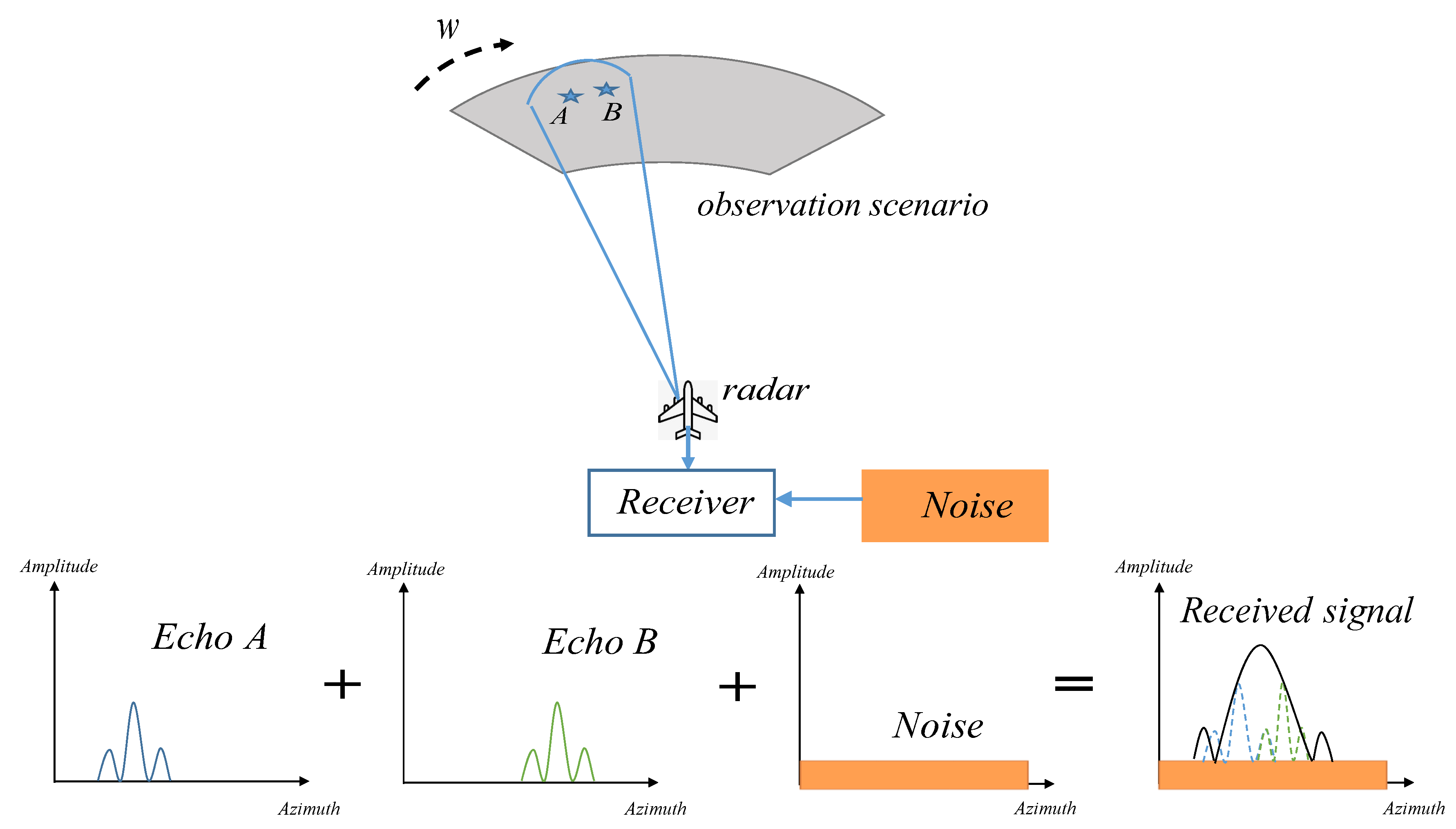
A radar system is required to emit electromagnetic waves to capture target information. The contradiction between the range resolution and the detection distance is resolved by transmitting a chirp signal, which is a kind of large time-bandwidth product signal. Employing mature pulse compression technology, we can achieve high range resolution. Therefore, improving azimuth resolution becomes the current task. Figure 1 illustrates the procedure of azimuth echoes acquisition. If the interval between the two targets is less than the beamwidth, the echoes of the two targets are added to get a composite echo. It can be clearly seen that due to antenna beam smoothing, the azimuth resolution becomes coarse.

The transmitted chirp signal is expressed:

$$s(\tau )=\mathrm{re}ct(\frac{\tau }{T_p})exp(j2\pi f_c\tau ).exp(j\pi k{\tau }^2),$$

(1)

where $\tau$ is range fast time, $T_p$ is the impulse width. $rect(\tau /T_p)=1,with\left|\tau \right|\le T_p/2$ and the other is 0. $f_c$ represents the signal carrier frequency, and k denotes the chirp rate.

In radar imaging, we usually treat the observation scene as a two-dimensional matrix, and each entry of the matrix is the reflectivity coefficients of the scatters.

$$\mathit{\sigma }=\left[\begin{array}{cccc}{\sigma }_{(x_1,y_1)}& {\sigma }_{(x_1,y_2)}& \cdots & {\sigma }_{(x_1,y_n)}\\ {\sigma }_{(x_2,y_1)}& {\sigma }_{(x_2,y_2)}& \cdots & {\sigma }_{(x_2,y_n)}\\ ⋮& ⋮& ⋮& ⋮\\ {\sigma }_{(x_m,y_1)}& {\sigma }_{(x_m,y_2)}& \cdots & {\sigma }_{(x_m,y_n)},\end{array}\right]$$

(2)

where m is the range dimension of the observed scene and n is the azimuth dimension of the observed scene. $\sigma {}_{(x_i{y}_j)}$ represents the backscattering coefficients of point $(x_i,y_j)$.

After the received echo is down-converted, it is expressed as:

$$\begin{array}{c}\begin{array}{c}s(\tau ,t)={\displaystyle \sum _{i=1}^m}{\displaystyle \sum _{j=1}^n}{\sigma }_{(x_i,y_j)}w(t-t_{(x_i,y_j)})rect(\frac{\tau -{\tau }_{(x_i,y_j)}}{T_p})exp(-j2\pi f_c{\tau }_{(x_i,y_j)})exp\left\{jk\pi {(\tau -{\tau }_{(x_i,y_j)})}^2\right\},\hfill \end{array}\hfill \end{array}$$

(3)

where t is azimuth slow time. $w(·)$ denotes the antenna pattern modulation and ${\tau }_{(x_i,y_j)}$ denotes the echo delay of point $(x_i,y_j)$.

Then range resolution is enhanced by pulse compression technology. For moving platform, due to the constant motion of the platform, echo signal is distributed in different range cells, hence range walk correction is necessary. After completing pulse compression and range walk correction in the frequency domain, the received echo is:

$$\begin{array}{c}\begin{array}{c}s(\tau ,t)={\displaystyle \sum _{i=1}^m}{\displaystyle \sum _{j=1}^n}{\sigma }_{(x_i,y_j)}w(t-t_{(x_i,y_j)})sinc\left\{B(\tau -{\tau }_{(x_i,y_j)})\right\}exp(-j2\pi f_c{\tau }_{(x_i,y_j)}),\hfill \end{array}\hfill \end{array}$$

(4)

where $exp(-j2\pi f_c{\tau }_{(x_i,y_j)})$ is the Doppler shift.

In a radar forward-looking area, the Doppler shift is usually negligible. After discarding the Doppler shift, we can discover that the echo is a two-dimensional convolution model. High range resolution has been realized, we only focus on the azimuth echo and rewrite it in matrix form.

$$\mathit{S}=\mathit{H}\mathit{\sigma }+\mathit{n}$$

(5)

where echo matrix $\mathit{S}$ and observed scene scattering coefficient matrix $\mathit{\sigma }$ are converted into a column vector. $\mathit{S}={[S_{11},S_{12},\cdots ,S_{1n},\cdots ,S_{mn}]}^H$ is the received echo vector, $\mathit{\sigma }={[{\sigma }_{11},{\sigma }_{12},\cdots ,{\sigma }_{1n},\cdots ,{\sigma }_{mn}]}^H$ is target scatter vector, $\mathit{n}={[n_{11},n_{12},\cdots ,n_{1n},\cdots ,n_{mn}]}^H$ is the additive white Gaussian noise. $\mathit{H}$ is the antenna pattern matrix composed of antenna pattern given by:

$$\begin{array}{c}\mathit{H}={\left[\begin{array}{cccc}{\mathit{H}}_{\mathbf{1}}& & & \\ & {\mathit{H}}_{\mathbf{1}}& & \\ & & \ddots & \\ & & & {\mathit{H}}_{\mathbf{1}}\end{array}\right]}_{mn\times mn}and\hfill \\ \\ {\mathit{H}}_{\mathbf{1}}={\left[\begin{array}{ccccc}{h}_0& \cdots & h_{-l}& & \\ ⋮& \ddots & & \ddots & \\ h_l& & \ddots & & h_{-l}\\ & \ddots & & \ddots & ⋮\\ & & h_l& \cdots & h_0\end{array}\right]}_{n\times n},\hfill \end{array}$$

(6)

where ${\mathit{H}}_{\mathbf{1}}$ is the antenna pattern modulation in one range cell. $\left[h_{-l}\cdots h_0\cdots h_l\right]$ is the sampling of the antenna pattern.

Through the above azimuth convolution model, we transform the azimuth super-resolution problem into a deconvolution problem. What we need to do is to recover the target scattering coefficient $\mathit{\sigma }$ accurately from the noisy echo $\mathit{S}$ with a known convolution kernel $\mathit{H}$ via deconvolution technique. Obviously, the deconvolution process is ill-posed, azimuth super-resolution is mathematically an ill-posed inversion problem.

3. The Proposed Method

In this section, the total variation method solved by iterative reweighted norm (IRN-TV) is first described, and then its high computational complexity is analyzed. Then, we derive the block tridiagonal structure of the matrix $\mathit{R}$. Finally, the fast total variation method based on iterative reweighted norm (IRN-FTV) is introduced in detail.

3.1. The Irn-Tv Method

Azimuth echo convolution model is as follows.

$$\mathit{S}=\mathit{H}\mathit{\sigma }+\mathit{n}.$$

(7)

Regularization strategy is one of the good ways to deal with ill-posed inverse problem. The regularization method replaces the original ill-posed problem with a problem that is close to well-conditioned by restricting the range of candidate solutions. The general form of standard regularization function [35,36] is:

$$T(\mathit{\sigma })=arg\underset{\mathit{\sigma }}{min}\frac{1}{p}{∥\mathit{H}\mathit{\sigma }-\mathit{S}∥}_p^p+\lambda \frac{1}{q}{∥\Gamma (\mathit{\sigma })∥}_q^q,$$

(8)

where the value of p, q depends on the norm type you choose. $\frac{1}{p}{∥\mathit{H}\mathit{\sigma }-\mathit{S}∥}_p^p$ is the data fitting term, $\frac{1}{q}{∥\Gamma (\mathit{\sigma })∥}_q^q$ is the adding regularization term or penalty term, $\lambda$ is a parameter that controls the trade off between the fidelity term and penalty term.

For maintaining the edge of the target, there are some other edge-preserving regularizers in References [37,38] besides the TV operator. But these new regularizers are mainly suitable for multi-spectral image or hyperspectral image rather than radar echo imagery, so this paper still adopts the TV operator. The TV operator has different forms, such as isotropic TV norm, anisotropic TV norm and smooth approximation TV norm [39]. According to the vectorized target scattering coefficient matrix and the Toplitz structure of the antenna measurement matrix, this paper constructs horizontal and vertical discrete gradient operators ${\mathit{D}}_{\mathit{x}}$ and ${\mathit{D}}_{\mathit{y}}$ in Equations (13) and (14) shown at the next page as regularization term. For $p=2$, $q=1$, the objection function is constructed as the following:

$$T(\mathit{\sigma })=arg\underset{\mathit{\sigma }}{min}{∥\mathit{H}\mathit{\sigma }-\mathit{S}∥}_2^2+\lambda {∥\sqrt{{\mathit{D}}_{\mathit{x}}\mathit{\sigma }+{\mathit{D}}_{\mathit{y}}\mathit{\sigma }}∥}_1,$$

(9)

where ${\mathit{D}}_{\mathit{x}}$ and ${\mathit{D}}_{\mathit{y}}$ are respectively horizontal and vertical discrete gradient operators.

Beforehand, we need to define ${\mathit{D}}_{\mathit{n}}$ in Equation (10). Then ${\mathit{D}}_{\mathit{n}}$ and Kronecker product are employed to define ${\mathit{D}}_{\mathit{x}}$ and ${\mathit{D}}_{\mathit{y}}$. ${\mathit{I}}_m$ is a $m\times m$ identity matrix, ⊗ is the Kronecker product.

$${\mathit{D}}_{\mathit{n}}={\left[\begin{array}{cccc}-1& 1& & \\ & \ddots & \ddots & \\ & & -1& 1\\ & & & -1\end{array}\right]}_{n\times n}.$$

(10)

Since the $L_1$ norm is not differentiable at the origin, the objective function minimum cannot be solved by the derivative method. Hence we use the iterative reweighted norm (IRN) approach, solving the minimum $L_1$ norm problem by solving a sequence of minimum weighted $L_2$ norm problem. We define the following matrices:

$$\mathit{D}=\left(\begin{array}{c}{\mathit{D}}_{\mathit{x}}\\ {\mathit{D}}_{\mathit{y}}\end{array}\right),\mathit{W}=\left(\begin{array}{cc}\Omega & 0\\ 0& \Omega \end{array}\right)$$

(11)

where $\Omega =diag({({({\mathit{D}}_{\mathit{x}}\mathit{\sigma })}^2+{({\mathit{D}}_{\mathit{y}}\mathit{\sigma })}^2)}^{-1/2})$, and ${({\mathit{D}}_{\mathit{x}}\mathit{\sigma })}^2=({\mathit{D}}_{\mathit{x}}\mathit{\sigma })\odot ({\mathit{D}}_{\mathit{x}}\mathit{\sigma })$, ${({\mathit{D}}_{\mathit{y}}\mathit{\sigma })}^2=({\mathit{D}}_{\mathit{y}}\mathit{\sigma })\odot ({\mathit{D}}_{\mathit{y}}\mathit{\sigma })$, ⊙ is dot product.

We use the iterative strategy to constantly update $\mathit{\sigma }$ and finally approach the true value. The iterative process, which is called the total variation super-resolution imaging method, is as follows:

$$\begin{array}{c}initialize:{\mathit{\sigma }}_0={({\mathit{H}}^T\mathit{H}+\lambda {\mathit{D}}^T\mathit{D})}^{-1}{\mathit{H}}^T\mathit{S}\hfill \\ \\ fork=0,1,2,\cdots \hfill \\ \\ {\Omega }_k=diag({({({\mathit{D}}_{\mathit{x}}{\mathit{\sigma }}_k)}^2+{({\mathit{D}}_{\mathit{y}}{\mathit{\sigma }}_k)}^2)}^{-1/2})\hfill \\ \\ {\mathit{W}}_k=\left(\begin{array}{cc}{\Omega }_k& 0\\ 0& {\Omega }_k\end{array}\right)\hfill \\ \\ {\mathit{\sigma }}_{k+1}={({\mathit{H}}^T\mathit{H}+\lambda {\mathit{D}}^T{\mathit{W}}_k\mathit{D})}^{-1}{\mathit{H}}^T\mathit{S}\hfill \\ ,end\hfill \end{array}$$

(12)

where k is iterations for convergence.

$${\mathit{D}}_{\mathit{x}}={\mathit{D}}_n\otimes {\mathit{I}}_m={\left[\begin{array}{ccccccc}-1& 0& \cdots & 1& & 0& \\ & -1& 0& \cdots & 1& & \\ & & \ddots & & & \ddots & \\ & & & \ddots & \ddots & & 1\\ & 0& & & \ddots & & ⋮\\ & & & & & \ddots & 0\\ & & & & & & -1\end{array}\right]}_{mn\times mn}$$

(13)

$${\mathit{D}}_{\mathit{y}}={\mathit{I}}_m\otimes {\mathit{D}}_{\mathit{n}}={\left[\begin{array}{ccc}{\left[\begin{array}{cccc}-1& 1& & \\ & \ddots & \ddots & \\ & & -1& 1\\ & & & 0\end{array}\right]}_{n\times n}& & 0\\ & \ddots & \\ 0& & {\left[\begin{array}{cccc}-1& 1& & \\ & \ddots & \ddots & \\ & & -1& 1\\ & & & 0\end{array}\right]}_{n\times n}\end{array}\right]}_{mn\times mn}.$$

(14)

Because the observed scene scattering coefficient matrix $\mathit{\sigma }$ and echo matrix $\mathit{S}$ are vectorized, the main computational burden of the IRN-TV method comes from matrix multiplication and inversion of ${({\mathit{H}}^T\mathit{H}+\lambda {\mathit{D}}^T\mathit{D})}^{-1}$ and ${({\mathit{H}}^T\mathit{H}+\lambda {\mathit{D}}^T{\mathit{W}}_k\mathit{D})}^{-1}$, which both are $O(m^3{n}^3)$. Because each iteration needs to update and calculate ${({\mathit{H}}^T\mathit{H}+\lambda {\mathit{D}}^T{\mathit{W}}_k\mathit{D})}^{-1}$, this is the root cause of slow running speed of the traditional IRN-TV method.

3.2. Block Tridiagonal Structure of the Matrix R

From the above analysis, we can see that the traditional IRN-TV method is slow due to the inversion and multiplication of large matrices in each iteration. Hence this paper mainly cares about how to improve the computational efficiency of ${({\mathit{H}}^T\mathit{H}+\lambda {\mathit{D}}^T\mathit{D})}^{-1}$ and ${({\mathit{H}}^T\mathit{H}+\lambda {\mathit{D}}^T{\mathit{W}}_k\mathit{D})}^{-1}$.

When ${\mathit{W}}_k=\mathit{I}$, $\mathit{I}$ is the identity matrix. We have

$${({\mathit{H}}^T\mathit{H}+\lambda {\mathit{D}}^T{\mathit{W}}_k\mathit{D})}^{-1}={({\mathit{H}}^T\mathit{H}+\lambda {\mathit{D}}^T\mathit{D})}^{-1}.$$

(15)

Therefore, this article pays concentration on ${({\mathit{H}}^T\mathit{H}+\lambda {\mathit{D}}^T{\mathit{W}}_k\mathit{D})}^{-1}$, the more general term.

Firstly, we define the matrix:

$$\mathit{U}{}_k={({({\mathit{D}}_{\mathit{x}}{\mathit{\sigma }}_k)}^2+{({\mathit{D}}_{\mathit{y}}{\mathit{\sigma }}_k)}^2)}^{-1/2},$$

(16)

and we can infer the following equations.

$$\begin{array}{c}{\Omega }_k=\mathrm{diag}(\mathit{U}{}_k)\hfill \end{array}$$

(17)

$$\begin{array}{c}\lambda {\mathit{D}}^T{\mathit{W}}_k\mathit{D}=\lambda {\mathit{D}}_{\mathit{x}}{\Omega }_k{\mathit{D}}_{\mathit{x}}+\lambda {\mathit{D}}_{\mathit{y}}{\Omega }_k{\mathit{D}}_{\mathit{y}}.\hfill \end{array}$$

(18)

The matrix ${\mathit{H}}^T\mathit{H}$ is block diagonal matrix with Toeplitz block:

$${\mathit{H}}^T\mathit{H}=\left[\begin{array}{cccc}{{\mathit{H}}_1}^T{\mathit{H}}_1& & & \\ & {{\mathit{H}}_1}^T{\mathit{H}}_1& & \\ & & \ddots & \\ & & & {{\mathit{H}}_1}^T{\mathit{H}}_1.\end{array}\right]$$

(19)

In addition, we find that the results of $\lambda {\mathit{D}}^T{\mathit{W}}_k\mathit{D}$ satisfy the structure of block tridiagonal matrix:

$$\begin{array}{c}\lambda {\mathit{D}}^T{\mathit{W}}_k\mathit{D}=\lambda {\mathit{D}}_{\mathit{x}}{\Omega }_k{\mathit{D}}_{\mathit{x}}+\lambda {\mathit{D}}_{\mathit{y}}{\Omega }_k{\mathit{D}}_{\mathit{y}}\hfill \\ =\left[\begin{array}{ccccc}{\mathit{A}}_1& {\mathit{B}}_2& & & \\ {\mathit{C}}_2& {\mathit{A}}_2& {\mathit{B}}_3& & \\ & {\mathit{C}}_3& {\mathit{A}}_3& \ddots & \\ & & \ddots & \ddots & {\mathit{B}}_m\\ & & & {\mathit{C}}_m& {\mathit{A}}_m,\end{array}\right]\hfill \end{array}$$

(20)

where each entry is a $n\times n$ square matrix.

For the convenience of description, let $\mathit{R}={\mathit{H}}^T\mathit{H}+\lambda {\mathit{D}}^T{\mathit{W}}_k\mathit{D}$. Thus the matrix $\mathit{R}$ is a sum of a diagonal block with banded Toeplitz block plus a special block tridiagonal correction.

$$\begin{array}{c}\mathit{R}=\left[\begin{array}{ccccc}{\mathit{A}}_1^{\prime }& {\mathit{B}}_2& & & \\ {\mathit{C}}_2& {\mathit{A}}_2^{\prime }& {\mathit{B}}_3& & \\ & {\mathit{C}}_3& {\mathit{A}}_3^{\prime }& \ddots & \\ & & \ddots & \ddots & {\mathit{B}}_m\\ & & & {\mathit{C}}_m& {\mathit{A}}_m^{\prime }.\end{array}\right]\hfill \end{array}$$

(21)

Assuming that $\mathit{U}=[u_{11},u_{12},\dots ,u_{1n},\dots u_{mn}{]}_{mn\times 1}^H$, the expression for each block matrix of $\mathit{R}$ is deduced in Equations (22), (24) and (25).

$${\mathit{B}}_i={\mathit{C}}_i=\lambda \left[\begin{array}{cccc}-u_{i1}& & & \\ & -u_{i2}& & \\ & & \ddots & \\ & & & -u_{in}\end{array}\right],i=2,3\dots ,m.$$

(22)

3.3. Irn-Ftv Method

The following task is to accelerate the inverse of $\mathit{R}$. Many methods for fast inversion using the block tridiagonal properties have been proposed [40,41,42]. In this paper, the method of twisted block decomposition is employed.

We assume that matrix $\mathit{X}$ is the inverse matrix of $\mathit{R}$.

$${\mathit{R}}^{-1}=\mathit{X}=\left[\begin{array}{cccc}{\mathit{X}}_{11}& {\mathit{X}}_{12}& \cdots & {\mathit{X}}_{1m}\\ {\mathit{X}}_{21}& {\mathit{X}}_{22}& \cdots & {\mathit{X}}_{2m}\\ ⋮& ⋮& ⋮& ⋮\\ {\mathit{X}}_{m1}& {\mathit{X}}_{m2}& \cdots & {\mathit{X}}_{mm},\end{array}\right]$$

(23)

where ${\mathit{X}}_{ij}(i=1,2,\cdots ,m;j=1,2,\cdots ,m)$ is a $n\times n$ square matrix.

The method of twisted block decomposition consists of four parts, which are detailed below.

$$\begin{array}{c}\begin{array}{c}{\mathit{A}}_1^{\prime }=\lambda \left[\begin{array}{ccccc}2u_{11}& -u_{11}& & & \\ -u_{1(j-1)}& 2u_{1j}+u_{1(j-1)}& -u_{1j}& & \\ & \ddots & \ddots & \ddots & \\ & & -u_{1(n-2)}& 2u_{1(n-1)}+u_{1(n-2)}& -u_{1(n-1)}\\ & & & -u_{1(n-1)}& u_{1n}+u_{1(n-1)}\end{array}\right]+{{\mathit{H}}_1}^T{\mathit{H}}_1;\hfill \\ j=2,3,\cdots ,n-1.\hfill \end{array}\hfill \end{array}$$

(24)

$$\begin{array}{c}\begin{array}{c}{\mathit{A}}_i^{\prime }=\lambda \left[\begin{array}{ccccc}{u}_{(i-1)1}+2u_{i1}& -u_{i1}& & & \\ -u_{i(j-1)}& 2u_{ij}+u_{i(j-1)}+u_{(i-1)j}& -u_{ij}& & \\ & \ddots & \ddots & \ddots & \\ & & -u_{i(n-2)}& 2u_{i(n-1)}+u_{i(n-2)}+u_{(i-1)(n-1)}& -u_{i(n-1)}\\ & & & -u_{i(n-1)}& u_{(i-1)n}+u_{in}+u_{i(n-1)}\end{array}\right]\hfill \\ +{{\mathit{H}}_1}^T{\mathit{H}}_1;\hfill \\ i=2,3,\dots m;j=2,3,\dots ,n-1\hfill \\ .\hfill \end{array}\hfill \end{array}$$

(25)

3.3.1. Initialization

We assume ${\mathit{B}}_{m+1}={\mathit{I}}_n,{\mathit{C}}_1={\mathit{I}}_n,{\mathit{K}}_{m+\mathbf{1}}={\mathit{O}}_n,\mathit{K}{}_0^{\prime }={\mathit{O}}_n$, where ${\mathit{I}}_n$ represents a $n\times n$ identity matrix, ${\mathit{O}}_n$ denotes a $n\times n$ zero matrix.

$\left\{{\mathit{K}}_i\right\}$ and $\left\{\mathit{K}{}_i^{\prime }\right\}$, $(i=0,1,2\cdots ,m+1)$ are auxiliary matrix sequences, and each entry of the sequences is a $n\times n$ square matrix.

3.3.2. Compute the Inverse of the $1_{St}$ Column

The inverse of the $1_{St}$ column ${\mathit{X}}_{i1}(i=1,2,\cdots m)$ can be expressed as:

$$\begin{array}{c}{\mathit{P}}_i={\mathit{A}}_i^{\prime }-{\mathit{B}}_{i+1}{\mathit{K}}_{i+1},{\mathit{K}}_i={{\mathit{P}}_i}^{-1}{\mathit{C}}_i(i=m,m-1,\dots ,1)\hfill \\ {\mathit{X}}_{11}={{\mathit{K}}_1}^{-1}\hfill \\ {\mathit{X}}_{i1}=-{\mathit{K}}_i{\mathit{X}}_{i-1,1}(i=2,3,\cdots m),\hfill \end{array}$$

(26)

where $\left\{{\mathit{P}}_i\right\}$ are the auxiliary matrix sequences as well as $\left\{{\mathit{K}}_i\right\}$.

3.3.3. Compute the Inverse of the $M_{Th}$ Column

Similarly, we have the inverse of the $M_{Th}$ column ${\mathit{X}}_{im}(i=m,m-1,\cdots 1)$:

$$\begin{array}{c}\mathit{P}{}_i^{\prime }={\mathit{A}}_i^{\prime }-{\mathit{C}}_i\mathit{K}{}_{i-1}^{\prime },\mathit{K}{}_i^{\prime }=\mathit{P}{{}_i^{\prime }}^{-1}{\mathit{B}}_{i+1}(i=1,2,\dots ,m)\hfill \\ {\mathit{X}}_{mm}=\mathit{P}{{}_m^{\prime }}^{-1}\hfill \\ {\mathit{X}}_{im}=-\mathit{K}{}_i^{\prime }{\mathit{X}}_{i+1,m}(i=m-1,m-2,\dots ,1),\hfill \end{array}$$

(27)

where $\left\{{\mathit{P}}_i^{\prime }\right\}$ are also the auxiliary matrix sequences.

3.3.4. Compute the Inverse of the $2_{Nd}$ to $M-1_{Th}$ Column

By the same way, we can easily deduce the following equations.

$$\begin{array}{c}{\mathit{X}}_{jj}={({\mathit{P}}_j-{\mathit{C}}_j\mathit{K}{}_{j-1}^{\prime })}^{-1}(j=2,3,\dots ,m-1)\hfill \\ {\mathit{X}}_{ij}=-{{\mathit{K}}_i}^{\prime }{\mathit{X}}_{i-1,j}(i=j-1,j-2,\dots ,1)\hfill \\ {\mathit{X}}_{ij}=-{\mathit{K}}_i{\mathit{X}}_{i-1,j}(i=j+1,j+2,\dots ,m).\hfill \end{array}$$

(28)

The twisted block decomposition approach converts the inverse of $\mathit{R}$ into computation of multiple small matrices, which reduces computational complexity and saves computation time. By introducing auxiliary matrix sequences, each column of $\mathit{R}$ satisfies an iterative formula. For each column, only the inverse of the initial element is required, and the inverse of other elements in this column can be deduced by a recursion formula. The algorithm contains $3m-2$ direct inverse of $n\times n$ matrix, $m^2+O(m)$ multiplications of $n\times n$ matrix, $3m-4$ additions of $n\times n$ matrix. So, the total complexity of twisted block decomposition approach is $(m^2+6m-6)n^3$. Obviously, the complexity of twisted block decomposition approach is less than that of the existing fast inversion algorithms for block tridiagonal matrix, as shown in

Table 1. Comparison of the computing complexity.

Inversion Approaches	Computing Complexity
Block Gaussian-Jordan Elimination	$\frac{1}{3}(m^3+\frac{3}{2}{m}^2+\frac{7}{6}m-2)n^3$
Block matrix catch up method	$(4m^2+m-3)n^3$
Meurant algorithm [41]	$(2m^2+16m-17)n^3$
The method in Reference [40]	$(2m^2+4m)n^3$
twisted block decomposition [34]	$(m^2+6m-6)n^3$

.

It is worth noting that in the actual implementation, we do not need to calculate the matrix $\mathit{R}$ via $\mathit{R}={\mathit{H}}^T\mathit{H}+\lambda {\mathit{D}}^T{\mathit{W}}_k\mathit{D}$. After calculating the vector $\mathit{U}$, the expression of entry of the matrix $\mathit{R}$ can be obtained according to the Equations (22)–(24). Exploiting these small block matrices ${{\mathit{A}}_i}^{\prime },{\mathit{B}}_i,{\mathit{C}}_i$, we apply the method of twisted block decomposition to realize the fast inverse of $\mathit{R}$.

In order to explain the inversion process explicitly, we package the entire process of fast inversion for ${({\mathit{H}}^T\mathit{H}+\lambda {\mathit{D}}^T{\mathit{W}}_k\mathit{D})}^{-1}$ into a function $\Psi (·)$, as shown in

Table 2. Fast Computation of ${\mathbf{R}}^{-1}$.

function $\mathbf{\Psi }(\mathbf{U})$

Input U

get each entry of R via Equations (22)–(24)

initialization: ${\mathbf{B}}_{m+1}={\mathbf{I}}_n,{\mathbf{C}}_1={\mathbf{I}}_n,{\mathbf{K}}_{m+1}={\mathbf{O}}_n,\mathbf{K}{}_0^{\prime }={\mathbf{O}}_n$

inversion of $1$st column:

Compute ${\mathbf{P}}_i={{\mathbf{A}}^{\prime }}_i-{\mathbf{B}}_{i+1}{\mathbf{K}}_{i+1},{\mathbf{K}}_i={{\mathbf{P}}_i}^{-1}{\mathbf{C}}_i(i=m,m-1,\cdots ,1)$

Compute ${\mathbf{X}}_{11}={{\mathbf{K}}_1}^{-1}$

Compute ${\mathbf{X}}_{i1}=-{\mathbf{K}}_i{\mathbf{X}}_{i-1,1}(i=2,3,\cdots ,m)$

inversion of $m$th column:

Compute $\mathbf{P}{}_i^{\prime }={{\mathbf{A}}^{\prime }}_i-{\mathbf{C}}_i\mathbf{K}{}_{i-1}^{\prime },\mathbf{K}{}_i^{\prime }=\mathbf{P}{{}_i^{\prime }}^{-1}{\mathbf{B}}_{i+1}(i=1,2,\cdots ,m)$

Compute ${\mathbf{X}}_{mm}=\mathbf{P}{{}_m^{\prime }}^{-1}$

Compute ${\mathbf{X}}_{im}=-\mathbf{K}{}_i^{\prime }{\mathbf{X}}_{i+1,m}(i=m-1,m-2,\cdots ,1)$

inversion of $2$nd to $m-1$th column:

Compute ${\mathbf{X}}_{jj}={({\mathbf{P}}_j-{\mathbf{C}}_j\mathbf{K}{}_{j-1}^{\prime })}^{-1}(j=2,3,\cdots ,m-1)$

Compute ${\mathbf{X}}_{ij}=-{{\mathbf{K}}_i}^{\prime }{\mathbf{X}}_{i-1,j}(i=j-1,j-2,\cdots ,1)$

Compute ${\mathbf{X}}_{ij}=-{\mathbf{K}}_i{\mathbf{X}}_{i-1,j}(i=j+1,j+2,\cdots ,m)$

${\mathbf{R}}^{-1}=\mathbf{X}$

end

. In this function, the vector $\mathit{U}$ is the input variable and ${\mathit{R}}^{-1}$ is the output.

Hence detailed process of the IRN-FTV method in this paper is as follows:

$$\begin{array}{c}{\mathit{U}}_0={{[1,1,\cdots ,1]}^T}_{mn\times 1}\hfill \\ \\ initialize:{\mathit{\sigma }}_0=\Psi ({\mathit{U}}_0){\mathit{H}}^T\mathit{S}\hfill \\ \\ fork=0,1,2,\cdots \hfill \\ \\ {\mathit{U}}_{k+1}={({({\mathit{D}}_{\mathit{x}}{\mathit{\sigma }}_k)}^2+{({\mathit{D}}_{\mathit{y}}{\mathit{\sigma }}_k)}^2)}^{-1/2}\hfill \\ \\ {\mathit{\sigma }}_{k+1}=\Psi ({\mathit{U}}_{k+1}){\mathit{H}}^T\mathit{S}\hfill \\ \\ .end\hfill \end{array}$$

(29)

Compared with the traditional IRN-TV method, our IRN-FTV method takes advantage of the block tridiagonal structure properties and accelerates the inversion process by way of twisted block decomposition. In addition, in the actual implementation process, our method only needs to calculate the vector $\mathit{U}$, which avoids large matrix-matrix multiplications. Our method effectively addresses the issue of multiplications and inversion of large matrices in each iteration and improves the computational efficiency of the IRN-TV method.

4. Simulations and Real Data Results

To verify the super-resolution imaging performance of the proposed method, the two-dimensional scene simulations are presented. We compare the imaging performance among fast total variation (FTV), total variation (TV), and some other super-resolution methods in References [6,8,14]. For the regularization methods involved, the regularization parameters are selected by the L-curve method [43], and the truncation parameters of the TSVD method are selected by the generalized cross validation (GCV) [44]. The number of iterations of the classical Lucy-Richardson method is chosen to be 20. To testify the contour preservation capability, experimental data will be employed. In addition, the computational complexity comparison between FTV and TV of different scanning scope will be investigated.

4.1. Two-Dimensional Scene Simulations

Indexes such as the relative error (RE) and beam sharpening ratio (BSR) are used in this section to quantify and compare the super-resolution performance and imaging quality of these super-resolution methods.

The relative error (RE) is defined as follows.

$$\mathrm{RE}=\frac{{∥{\mathit{\sigma }}_k-\mathit{\sigma }∥}_2^2}{{∥\mathit{\sigma }∥}_2^2},$$

(30)

where ${\mathit{\sigma }}_k$ denotes the obtained super-resolution result, and $\mathit{\sigma }$ is the original scene. RE is a quantitative measure between the super-resolution result and the original target scattering coefficient distribution. The smaller the value of RE, the closer match the recovery target scene exhibits with the original scene.

The beam sharpening ratio (BSR) is defined as the ratio that the original real beam 3dB bandwidth divides super-resolution processing result 3dB bandwidth, shown in Figure 2.

$$\mathrm{BSR}=\frac{{\theta }_r}{{\theta }_s},$$

(31)

where BSR measures the ability of super-resolution, the larger BSR indicates higher resolution ability.

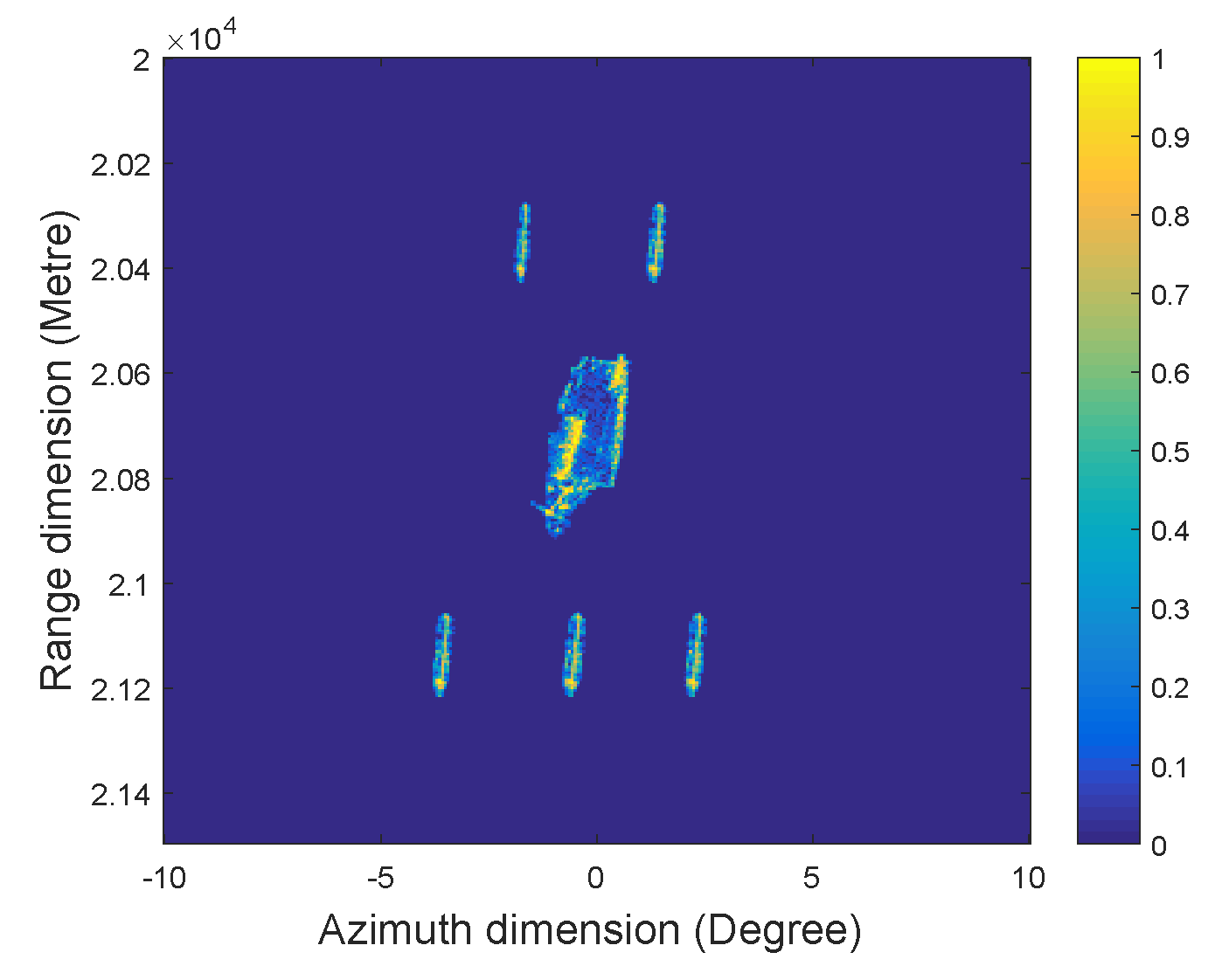
The two-dimensional scene is shown in Figure 3. The fleet of 5 warships and 1 carrier and the materials come from synthetic aperture radar imaging. The system parameters are listed in

Table 3. The 2-D Simulation Parameters.

Parameter	Value
Carrier frequency	30.75 GHz
Bandwidth	40 MHz
Antenna scanning speed	30${}^{\circ }/$s
Main beamwidth	5${}^{\circ }$
Pulse repetition frequency	1000 Hz
Scanning area	−10${}^{\circ }$∼10${}^{\circ }$

.

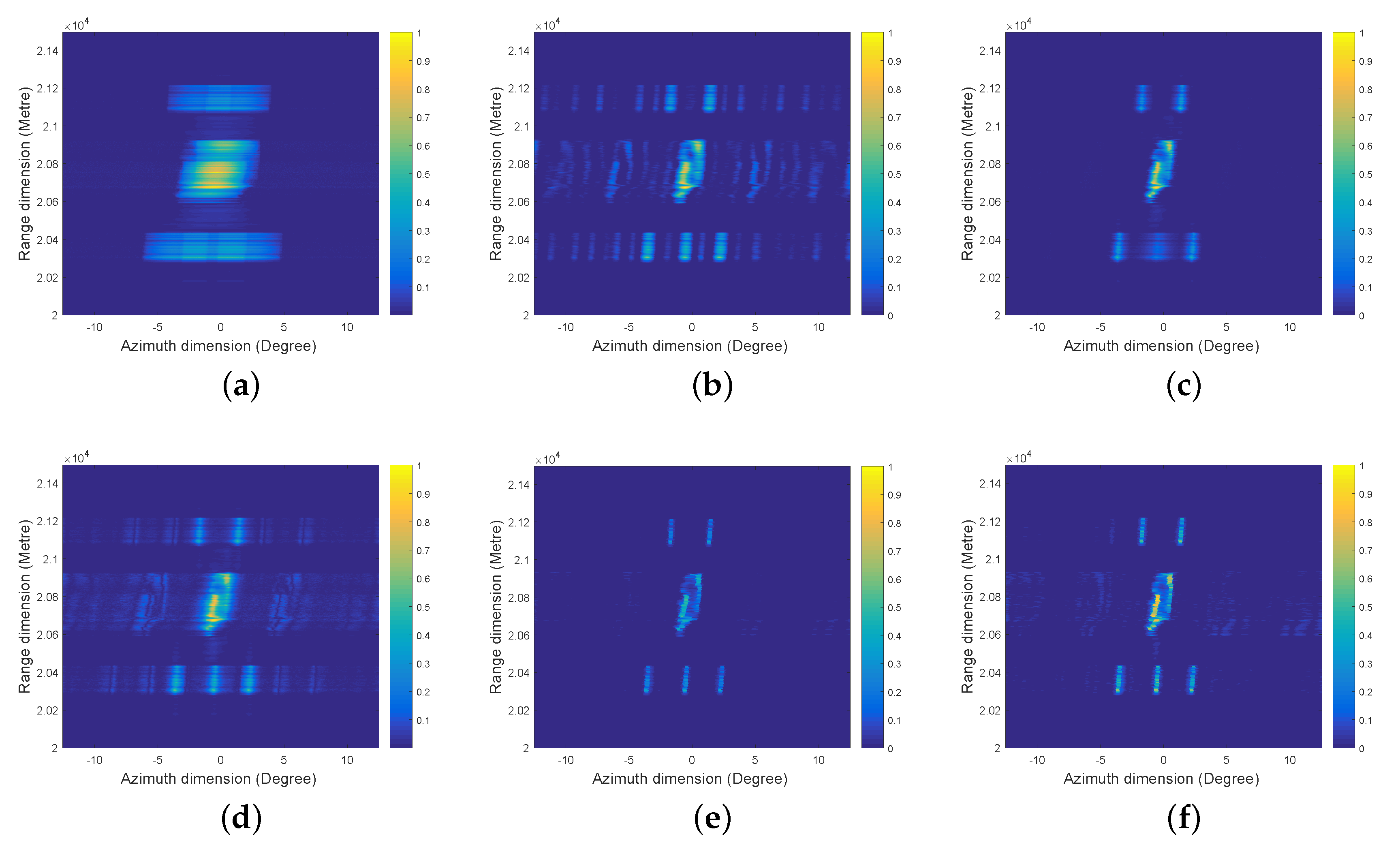
When the signal to noise ratio (SNR) is 25 dB, the real beam result is shown in Figure 4a. We can see that it suffers from coarse azimuth resolution with little valuable information. Figure 4b displays the result processed by the TSVD method. Although it improves the azimuth resolution to a certain degree, it brings a lot of noise, which influences the image quality. In addition, the outline of the aircraft carrier becomes blurred. Figure 4c suppresses noise by Lucy-Richardson method, but the resolution is restricted, the warship below the aircraft carrier is not clear. Figure 4d gives the result processed by $L_2$ norm regularization method, it has a high noise level and the resolution improvement is finite. Carrier’s outline information has been partially lost. Obviously, observing Figure 4e,f, TV and FTV technology not only improves the resolution but also provides clear details of the original scene. In Figure 4e,f, 5 warships are clearly distinguished, and the restored image visual quality is higher than other methods. TV and FTV methods keep clearer contour details of the aircraft carrier than others, which is beneficial to detection and recognition. As can be seen from

Table 4. The Comparison of RE and BSR.

Method	RE	BSR
TSVD [13]	1.1311	5.25
Lucy-Richardson [6]	1.0367	7.00
$L_2$ norm regularization [8]	1.1523	5.73
TV [35]	0.9947	12.60
FTV	0.9949	12.60

, the TV and FTV have the smaller relative error (RE) than other approaches.

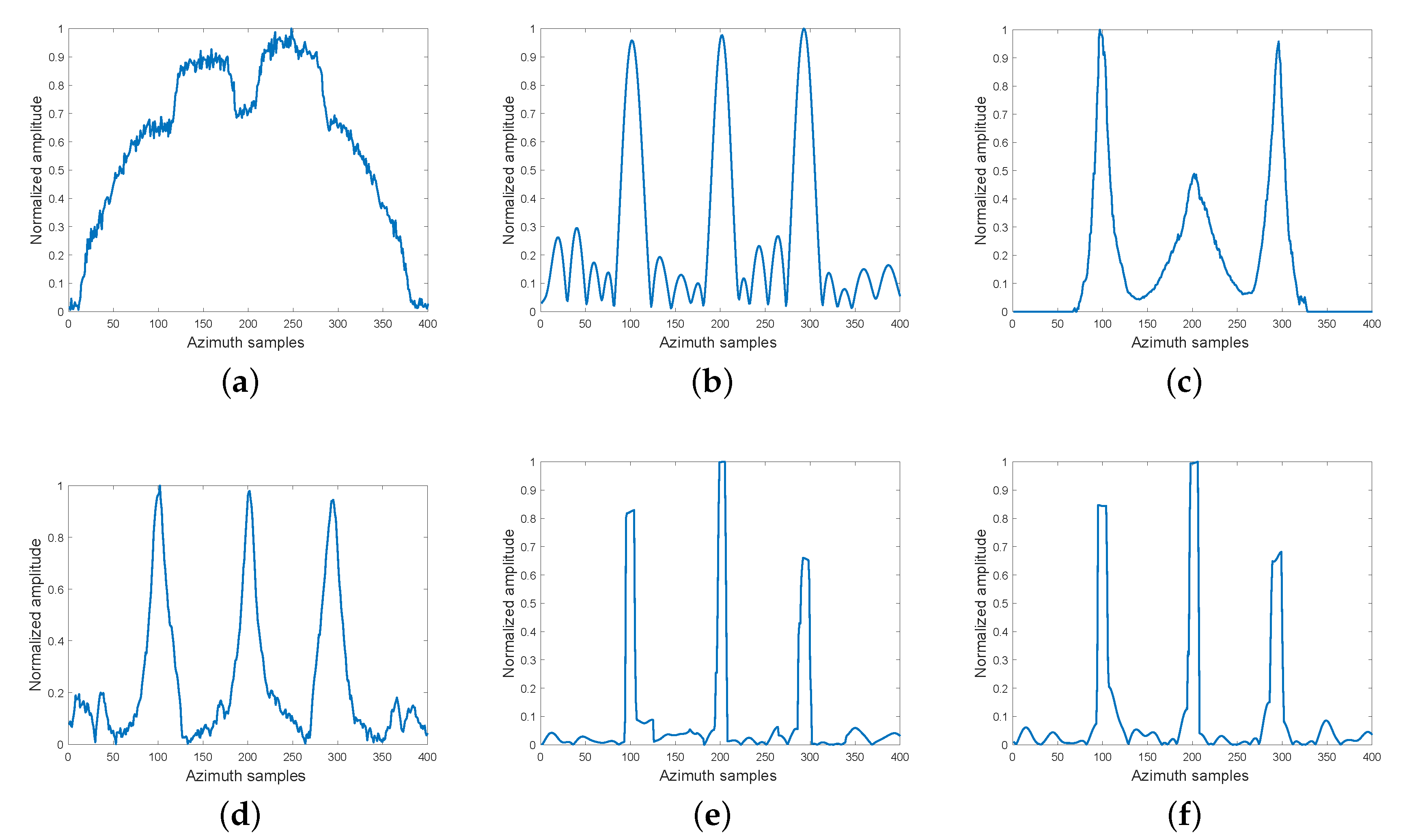
To quantitatively verify the super-resolution performance of the above methods, the profiles result of three warships below the aircraft carrier are illustrated in Figure 5. Due to the smoothing of the antenna pattern, the real beam echoes of three warships are overlapped and added to get a composite response. TSVD method and $L_2$ norm regularization method both improve azimuth resolution, but contain high sidelobe noise which affects the quality of imaging result. Lucy-Richardson method suppresses the sidelobe noise, but the beam sharpening effect is limited. TV and FTV methods have higher beam sharpening ability than other methods, and the noise is weak. From Table 4, the TV and FTV perform better in terms of BSR, which indicates that they have superior super-resolution capability than other approaches.

4.2. Experimental Data

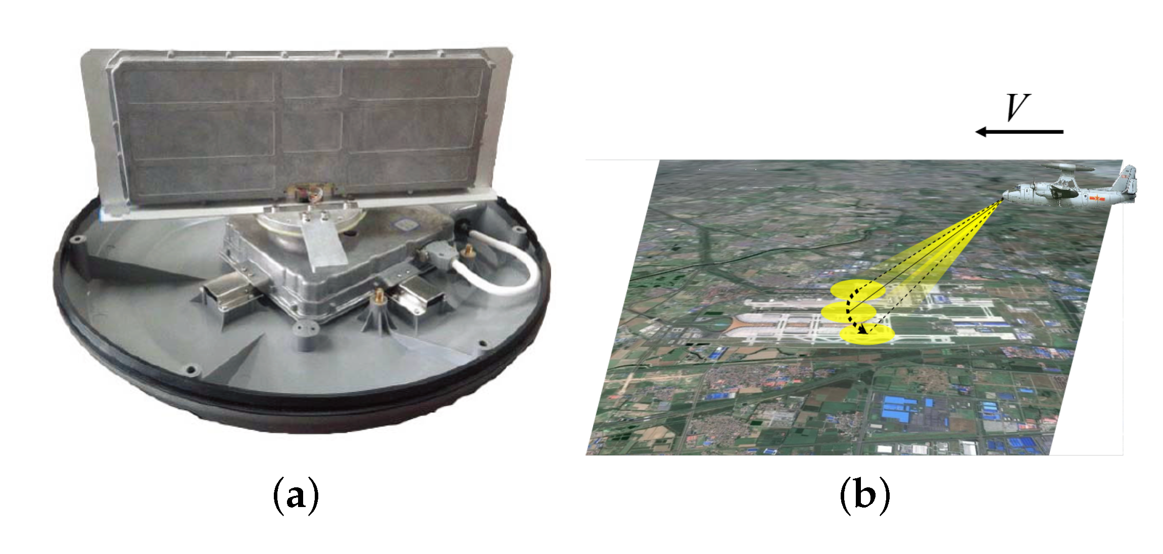
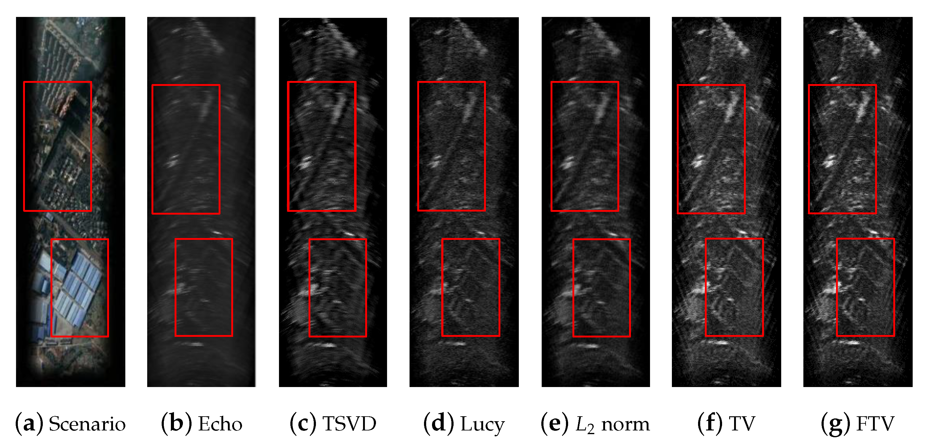
To further verify the contour preservation capability of various methods, airborne experimental data are utilized. The millimeter-wave radar and forward-looking scanning imaging mode are illustrated in Figure 6a,b. The radar of Figure 6a was fixed on the helicopter. The helicopter sweeps observation scene in forward-looking area that obtains experimental data depicted in Figure 6b. The experiment was conducted in Luodai Town, Chengdu, Sichuan, China. Figure 7a shows the optical scenario of experimental area, which is intercepted from Google Earth. In this scenario, we are concerned about two valuable typical areas characterized by adjacent houses and road, respectively. The system parameters of airborne experiment are listed in

Table 5. Experimental Parameters.

Parameter	Value
Signal carrier frequency	30.75 GHz
Band width	200 MHz
Antenna scanning speed	60${}^{\circ }/$s
Main beamwidth	4${}^{\circ }$
Pulse width	1 μs
Pulse repetition frequency	500 Hz
Height	189 m
Flight speed	37 m/s
depression angle	20${}^{\circ }$

.

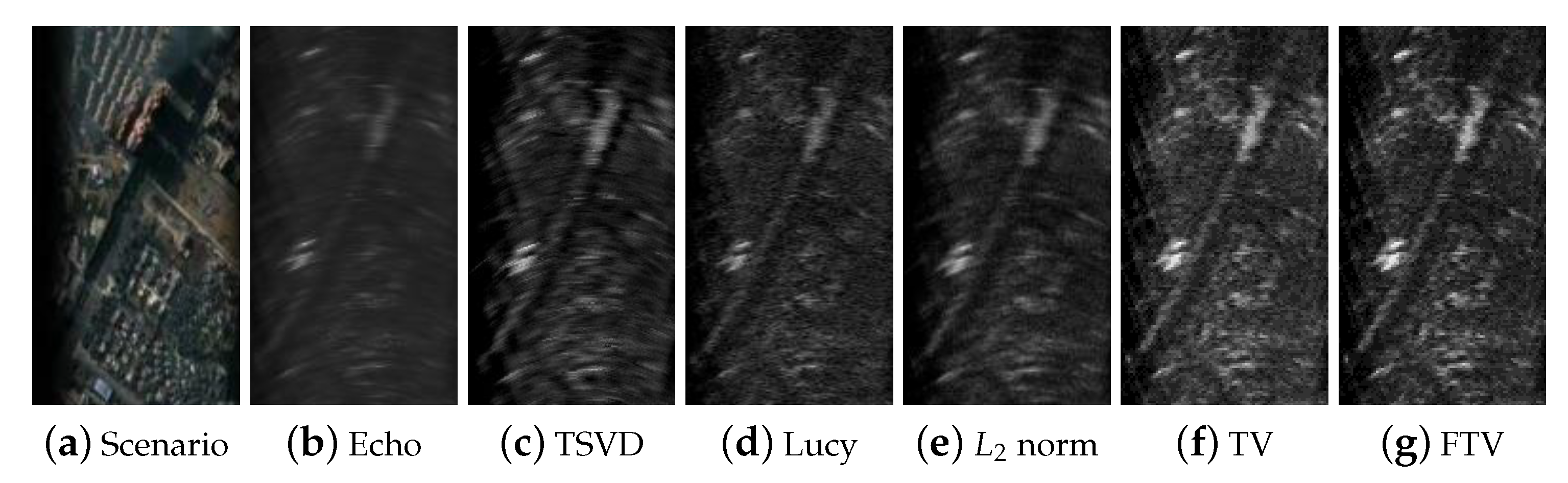
Figure 7 shows the experiment results. Figure 7b displays that the echo image, which encounters coarse azimuth resolution, and the adjacent houses and road are visually obscure. As observed in Figure 7c–e, the TSVD method, Lucy-Richardson method, and $L_2$ norm regularization method all improve the imaging resolution compared with the echo image, but imaging results are not distinct. In contrast, TV method and FTV method provide clearer outline features to adjacent houses and road than other methods, as shown in Figure 7f,g. Figure 8 and Figure 9 provide enlarged results for houses and roads, respectively. Obviously, they show that the images processed by the TV method and the FTV method are quite competitive over these other algorithms in terms of imaging visual quality and outline preservation.

4.3. Computational Complexity Comparison

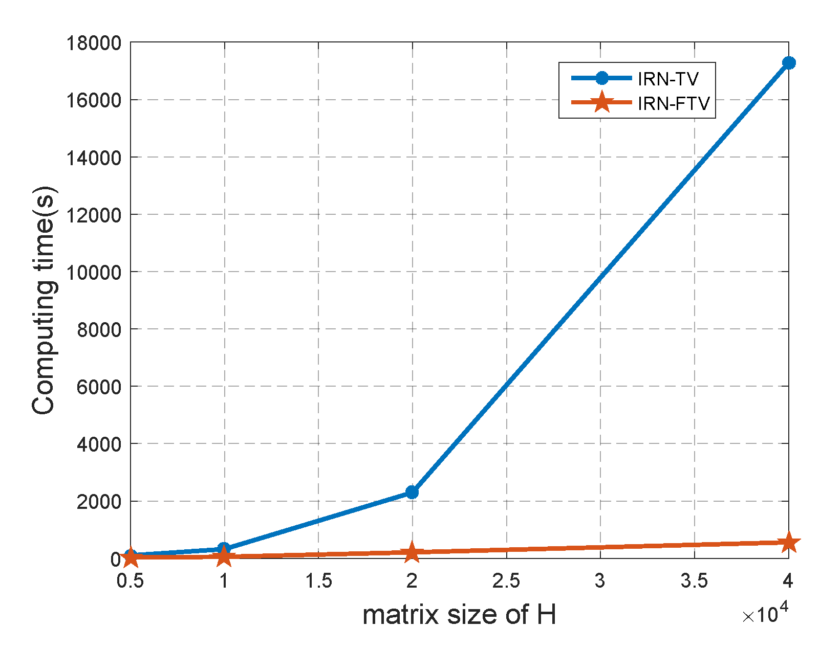
The computational complexity of IRN-TV and IRN-FTV with varying scanning scope will be investigated. Correspondingly, the azimuth sample n also varies. Pulse repetition frequency (PRF) is 500 Hz, and antenna scanning speed is 30${}^{\circ }/$s. For the sake of convenience, our range sample m is 100. The computational time of IRN-TV and IRN-FTV, referred to as $t_{IRN-TV}$ and $t_{IRN-FTV}$, respectively. The time rate (TR) is defined as $TR=t_{IRN-TV}/t_{IRN-FTV}$, which reflects improvement of algorithm computing efficiency. Simulation hardware and software environment are shown in

Table 6. The Simulation Conditions.

Hardware or Software	Parameters
CPU	Inter(R) Xeon(R) CPU E5-2680
RAM	256 GB
Platform	MATLAB 2015b

.

From Figure 10, we can see that the computational time curve of IRN-TV rises rapidly with the increase of matrix size, and the computational time curve of IRN-FTV grows slowly and is far lower than the curve of IRN-TV. We can observe from

Table 7. The comparison of computation time.

Scanning Scope	n	m	Matrix Size of H	${\mathit{t}}_{\mathit{IRN}-\mathit{TV}}$(s)	${\mathit{t}}_{\mathit{IRN}-\mathit{FTV}}$(s)	$\mathit{TR}$
$-{1.5}^{\circ }\mathrm{to}{1.5}^{\circ }$	50	100	5000	102.78	30.52	3.34
$-3^{\circ }\mathrm{to}{3}^{\circ }$	100	100	10,000	322.71	54.41	5.93
$-6^{\circ }\mathrm{to}{6}^{\circ }$	200	100	20,000	2297.2	210.52	10.91
$-{12}^{\circ }\mathrm{to}{12}^{\circ }$	400	100	40,000	17,280.41	558.76	30.92

that, as scanning scope increases, the matrix size of $\mathit{H}$ continues to enhance, and computational savings provided by IRN-FTV become more significant compared with the IRN-TV method.

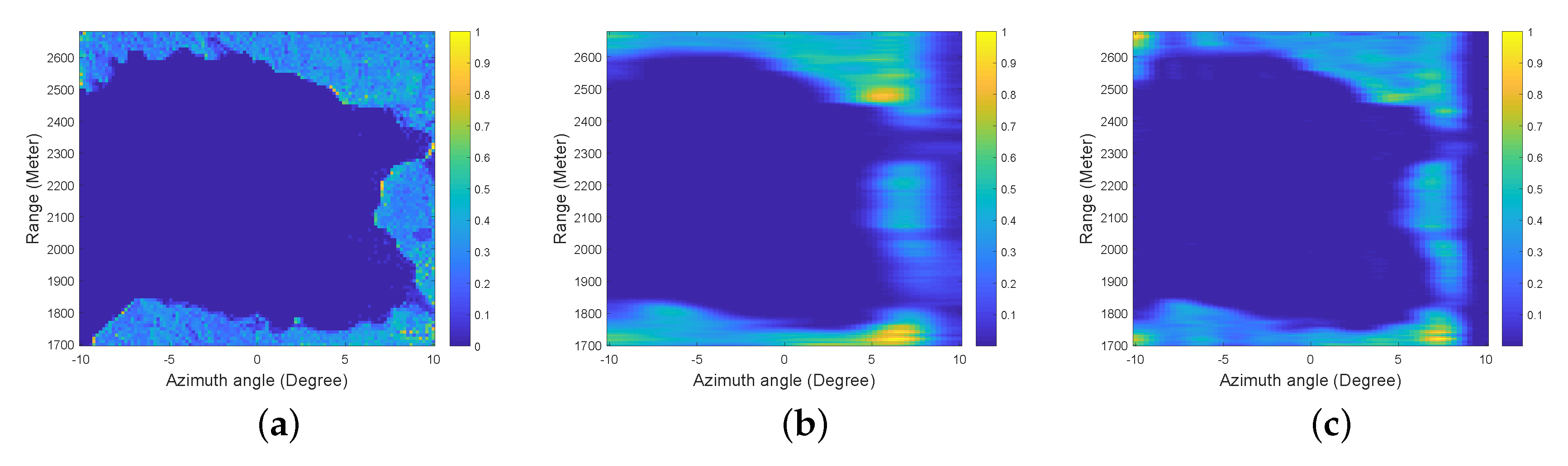
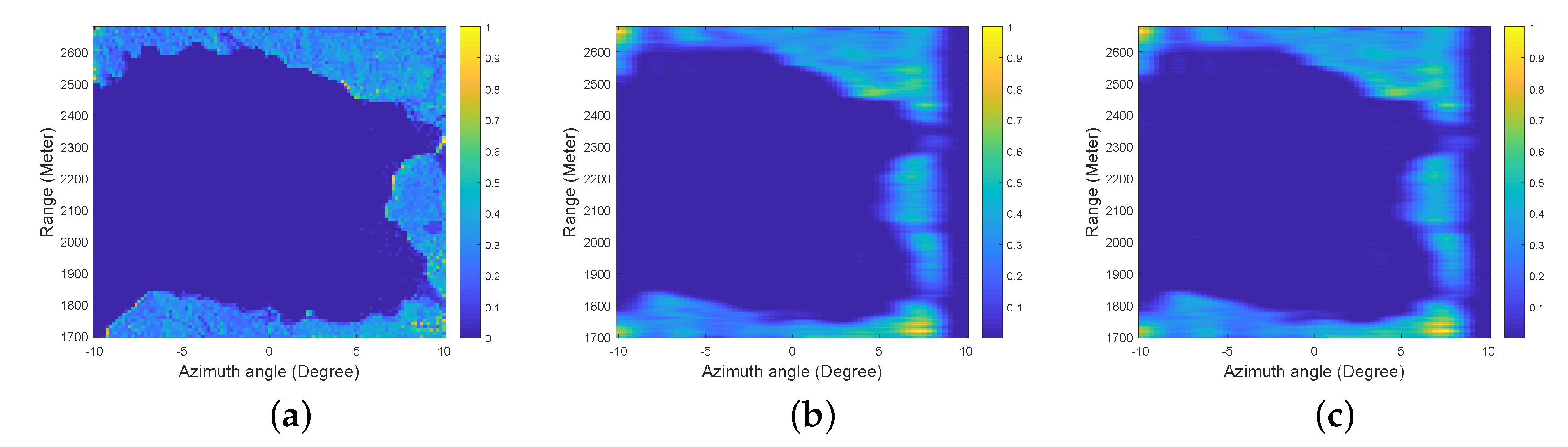
In order to verify the computation time—time is an important factor that affects the algorithm result—we give the following simulations. The simulation parameters are shown in

Table 8. Experimental Parameters.

Parameter	Value
Carrier frequency	10 GHz
Band width	200 MHz
Antenna scanning speed	30${}^{\circ }/$s
Main beamwidth	2.5${}^{\circ }$
Pulse width	2 μs
Pulse repetition frequency	100 Hz

and the hardware and software environments are the same as in Table 6. The simulation scene with size $99\times 111$ is shown in Figure 11a, which is a bay with a clear outline. When the running time of TV and FTV are the same, the proposed FTV method has a clearer outline and a higher degree of matching with the original scenario. Therefore, in order to achieve the same performance, the TV method needs to pay a higher time cost as shown in Figure 12.

5. Conclusions

In this paper, a fast total variation (FTV) algorithm solved by iterative reweighted norm (IRN) for airborne scanning radar super-resolution imaging is presented. By analyzing the traditional total variation (TV) method, we find that the main reason of its slow running speed is the high-dimensional matrix multiplication and inverse in each iteration.

Exploiting the structural property of the high-dimensional matrix with inverse, we convert the high-dimensional matrix with inverse into multiple small block matrices and apply the approach of twisted decomposition to accelerate its inversion. In addition, in the actual implementation process, our method avoids multiplications of high-dimensional matrices by deducing the explicit formula of each small block matrix.

Simulation and airborne experimental data results indicate that the superresolution imaging performance of our method will not degrade compared with the traditional TV method. The numerical results illustrate that the proposed IRN-FTV method offers a time complexity reduction especially for high-dimensional observation scenes.

The advantage of the proposed method is mainly for targets with a clear outline or extended point targets with a distinct edge. If the target is too sparse relative to the scene, then the target can be regarded as an isolated point, the advantage of the proposed method will not exist. Generally, the proposed method is suitable for a target with a clear contour in a dense scenario, such as houses in experimental data results.

References

- Sethmann, R.; Burns, B.A.; Heygster, G.C. Spatial resolution improvement of ssm/i data with image restoration techniques. IEEE Trans. Geosci. Remote Sens. 1994, 32, 1144–1151. [Google Scholar] [CrossRef]
- Elachi, C.; Brown, W.E., Jr. Imaging and sounding of ice fields with airborne coherent radars. J. Geophys. Res. 1975, 80, 1113–1119. [Google Scholar] [CrossRef]
- Piles, M.; Camps, A.; Vall-Llossera, M.; Talone, M. Spatial-resolution enhancement of smos data: A deconvolution-based approach. IEEE Trans. Geosci. Remote Sens. 2009, 47, 2182–2192. [Google Scholar] [CrossRef]
- Lenti, F.; Nunziata, F.; Estatico, C.; Migliaccio, M. Spatial resolution enhancement of earth observation products using an acceleration technique for iterative methods. IEEE Geosci. Remote Sens. Lett. 2014, 12, 269–273. [Google Scholar] [CrossRef]
- Zhang, Y.; Zhang, Q.; Zhang, Y.; Pei, J.; Huang, Y.; Yang, J. Fast split bregman based deconvolution algorithm for airborne radar imaging. Remote Sens. 2020, 12, 1747. [Google Scholar] [CrossRef]
- Zhou, D.; Huang, Y.; Yang, J. Radar angular superresolution algorithm based on bayesian approach. In Proceedings of the IEEE 10th International Conference on Signal Processing Proceedings, Beijing, China, 24–28 October 2010; pp. 1894–1897. [Google Scholar]
- Zhang, Q.; Zhang, Y.; Huang, Y.; Zhang, Y. Azimuth superresolution of forward-looking radar imaging which relies on linearized bregman. IEEE J. Sel. Top. Appl. Earth Obs. Remote Sens. 2019, 12, 2032–2043. [Google Scholar] [CrossRef]
- Gambardella, A.; Migliaccio, M. On the superresolution of microwave scanning radiometer measurements. IEEE Geosci. Remote Sens. Lett. 2008, 5, 796–800. [Google Scholar] [CrossRef]
- Gaikovich, K.; Zhilin, A. Tikhonov’s algorithm for two-dimensional image retrieval. Proc. Int. Conf. MMET 1998, 2, 622–624. [Google Scholar]
- Çetin, M.; Karl, W.C. Feature-enhanced synthetic aperture radar image formation based on nonquadratic regularization. IEEE Trans. Image Process. 2001, 10, 623–631. [Google Scholar] [CrossRef] [Green Version]
- Rao, W.; Li, G.; Wang, X.; Xia, X.-G. Adaptive sparse recovery by parametric weighted l _{1} minimization for isar imaging of uniformly rotating targets. IEEE J. Sel. Top. Appl. Earth Obs. Remote Sens. 2012, 6, 942–952. [Google Scholar] [CrossRef]
- Wu, Y.; Zhang, Y.; Mao, D.; Huang, Y.; Yang, J. Sparse super-resolution method based on truncated singular value decomposition strategy for radar forward-looking imaging. J. Appl. Remote Sens. 2018, 12, 035021. [Google Scholar]
- Lenti, F.; Nunziata, F.; Migliaccio, M.; Rodriguez, G. Two-dimensional tsvd to enhance the spatial resolution of radiometer data. IEEE Trans. Geosci. Remote Sens. 2013, 52, 2450–2458. [Google Scholar] [CrossRef]
- Shea, J.D.; van Veen, B.D.; Hagness, S.C. A tsvd analysis of microwave inverse scattering for breast imaging. IEEE Trans. Biomed. Eng. 2011, 59, 936–945. [Google Scholar] [CrossRef] [PubMed] [Green Version]
- Fang, Q.; Meaney, P.M.; Paulsen, K.D. Singular value analysis of the jacobian matrix in microwave image reconstruction. IEEE Trans. Antennas Propag. 2006, 54, 2371–2380. [Google Scholar] [CrossRef]
- Barrière, P.-A.; Idier, J.; Goussard, Y.; Laurin, J.-J. Fast solutions of the 2d inverse scattering problem based on a tsvd approximation of the internal field for the forward model. IEEE Trans. Antennas Propag. 2010, 58, 4015–4024. [Google Scholar] [CrossRef]
- Yardibi, T.; Li, J.; Stoica, P.; Xue, M.; Baggeroer, A.B. Source localization and sensing: A nonparametric iterative adaptive approach based on weighted least squares. IEEE Trans. Aerosp. Electron. Syst. 2010, 46, 425–443. [Google Scholar] [CrossRef]
- Roberts, W.; Stoica, P.; Li, J.; Yardibi, T.; Sadjadi, F.A. Iterative adaptive approaches to mimo radar imaging. IEEE J. Sel. Signal Process. 2010, 4, 5–20. [Google Scholar] [CrossRef]
- Stoica, P.; Li, J.; Ling, J.; Cheng, Y. Missing data recovery via a nonparametric iterative adaptive approach. In Proceedings of the 2009 IEEE International Conference on Acoustics, Speech and Signal Processing, Taipei, Taiwan, 19–24 April 2009; pp. 3369–3372. [Google Scholar]
- Yardibi, T.; Li, J.; Stoica, P. Nonparametric and sparse signal representations in array processing via iterative adaptive approaches. In Proceedings of the 2008 42nd Asilomar Conference on Signals, Systems and Computers, Pacific Grove, CA, USA, 26–29 October 2008; pp. 278–282. [Google Scholar]
- Zhang, Y.; Zhang, Y.; Li, W.; Huang, Y.; Yang, J. Super-resolution surface mapping for scanning radar: Inverse filtering based on the fast iterative adaptive approach. IEEE Trans. Geosci. Remote 2017, 56, 127–144. [Google Scholar] [CrossRef]
- Zhang, Q.; Zhang, Y.; Huang, Y.; Zhang, Y.; Li, W.; Yang, J. Total variation superresolution method for radar forward-looking imaging. In Proceedings of the 2019 6th Asia-Pacific Conference on Synthetic Aperture Radar (APSAR), Xiamen, China, 26–29 November 2019; pp. 1–4. [Google Scholar]
- Chambolle, A.; Darbon, J. On total variation minimization and surface evolution using parametric maximum flows. Int. J. Comput. Vis. 2009, 84, 288. [Google Scholar] [CrossRef] [Green Version]
- Oliveri, G.; Anselmi, N.; Massa, A. Compressive sensing imaging of non-sparse 2d scatterers by a total-variation approach within the born approximation. IEEE Trans. Antennas Propag. 2014, 62, 5157–5170. [Google Scholar] [CrossRef]
- van den Berg, P.M.; Kleinman, R.E. A total variation enhanced modified gradient algorithm for profile reconstruction. Inverse Probl. 1995, 11, L5. [Google Scholar] [CrossRef]
- Yaswanth, K.; Khankhoje, U.K. Two-dimensional non-linear microwave imaging with total variation regularization. In Proceedings of the 2017 Progress in Electromagnetics Research Symposium-Fall (PIERS-FALL), Singapore, 19–22 November 2017; pp. 1509–1513. [Google Scholar]
- Wilson, J.; Patwari, N.; Vasquez, F.G. Regularization methods for radio tomographic imaging. In Proceedings of the 2009 Virginia Tech Symposium on Wireless Personal Communications, Blacksburg, VA, USA, 3–5 June 2009; pp. 7–13. [Google Scholar]
- Zhang, Y.; Tuo, X.; Huang, Y.; Yang, J. A tv forward-looking super-resolution imaging method based on tsvd strategy for scanning radar. IEEE Trans. Geosci. Remote Sens. 2020, 58, 4517–4528. [Google Scholar] [CrossRef]
- Wohlberg, B.; Rodriguez, P. An iteratively reweighted norm algorithm for minimization of total variation functionals. IEEE Signal Process. Lett. 2007, 14, 948–951. [Google Scholar] [CrossRef]
- Rodríguez, P.; Wohlberg, B. Efficient minimization method for a generalized total variation functional. IEEE Trans. Image Process. 2008, 18, 322–332. [Google Scholar] [CrossRef]
- Chan, T.F.; Golub, G.H.; Mulet, P. A nonlinear primal-dual method for total variation-based image restoration. SIAM J. Sci. 1999, 20, 1964–1977. [Google Scholar] [CrossRef] [Green Version]
- Wu, C.; Tai, X.-C. Augmented lagrangian method, dual methods, and split bregman iteration for rof, vectorial tv, and high order models. SIAM J. Imaging Sci. 2010, 3, 300–339. [Google Scholar] [CrossRef] [Green Version]
- Getreuer, P. Total variation inpainting using split bregman. Image Process. Line 2012, 2, 147–157. [Google Scholar] [CrossRef] [Green Version]
- Ran, R.-S.; Huang, T.-Z. The inverses of block tridiagonal matrices. Appl. Math. Comput. 2006, 179, 243–247. [Google Scholar] [CrossRef]
- Wu, Y.; Zhang, Y.; Zhang, Y.; Huang, Y.; Yang, J. Outline reconstruction for radar forward-looking imaging based on total variation functional deconvloution methodxs. In Proceedings of the IGARSS 2018—2018 IEEE International Geoscience and Remote Sensing Symposium, Valencia, Spain, 22–27 July 2018; pp. 7267–7270. [Google Scholar]
- Rodriguez, P.; Wohlberg, B. An iteratively reweighted norm algorithm for total variation regularization. In Proceedings of the 2006 Fortieth Asilomar Conference on Signals, Systems and Computers, Pacific Grove, CA, USA, 29 October–1 November 2006; pp. 892–896. [Google Scholar]
- Lanaras, C.; Bioucas-Dias, J.; Baltsavias, E.; Schindler, K. Super-resolution of multispectral multiresolution images from a single sensor. In Proceedings of the IEEE Conference on Computer Vision and Pattern Recognition Workshops, Honolulu, HI, USA, 21–26 July 2017; pp. 20–28. [Google Scholar]
- Lin, C.-H.; Bioucas-Dias, J.M. An explicit and scene-adapted definition of convex self-similarity prior with application to unsupervised sentinel-2 super-resolution. IEEE Trans. Geosci. Remote 2019, 58, 3352–3365. [Google Scholar] [CrossRef]
- Song, X.; Xu, Y.; Dong, F. A hybrid regularization method combining tikhonov with total variation for electrical resistance tomography. Flow Meas. Instrum. 2015, 46, 268–275. [Google Scholar] [CrossRef]
- Du, Y.; Lu, Q.; Xu, Z. New algorithm for inversing block periodic tridiagonal matrices. Jisuanji Gongcheng Yingyong (Comput. Eng. Appl.) 2012, 48, 41–43. [Google Scholar]
- Meurant, G. A review on the inverse of symmetric tridiagonal and block tridiagonal matrices. SIAM J. Matrix Anal. Appl. 1992, 13, 707–728. [Google Scholar] [CrossRef] [Green Version]
- Reuter, M.G.; Hill, J.C. An efficient, block-by-block algorithm for inverting a block tridiagonal, nearly block toeplitz matrix. Comput. Sci. Discov. 2012, 5, 014009. [Google Scholar] [CrossRef] [Green Version]
- Hansen, P.C.; Leary, D.P.O. The use of the l-curve in the regularization of discrete ill-posed problems. SIAM J. Sci. Comput. 1993, 14, 1487–1503. [Google Scholar] [CrossRef]
- Golub, G.H.; Heath, M.; Wahba, G. Generalized cross-validation as a method for choosing a good ridge parameter. Technometrics 1979, 21, 215–223. [Google Scholar] [CrossRef]
Figure 1.
Azimuth signal model of airborne radar.
Figure 2.
The definition of beam sharpening ratio (BSR).
Figure 3.
The two-dimensional scene.
Figure 4.
The 2-D simulation result. (a) The echo; (b) The truncated singular value decomposition (TSVD) method; (c) The Lucy-Richardson method; (d) The norm regularization method; (e) The total variation (TV) method; (f) The proposed fast total variation (FTV) method.
Figure 5.
The profiles result of three warships below the aircraft carrier. (a) The echo; (b) The TSVD method; (c) The Lucy-Richardson method; (d) The norm regularization method; (e) The TV method; (f) The proposed FTV method.
Figure 6.
The experiment system and imaging model. (a) The millimeter-wave radar; (b) The forward-looking scanning imaging model.
Figure 7.
The experimental data result. (a) Optical scenario; (b) Echo image; (c) The TSVD method result; (d) The Lucy-Richardson method result; (e) The norm regularization method result; (f) The TV method result; (g) The proposed FTV method result.
Figure 8.
Partially enlarged results for houses. (a) Optical scenario; (b) Echo image; (c) The TSVD method result; (d) The Lucy-Richardson method result; (e) The norm regularization method result; (f) The TV method result; (g) The proposed FTV method result.
Figure 9.
Partially enlarged results for road. (a) Optical scenario; (b) Echo image; (c) The TSVD method result; (d) The Lucy-Richardson method result; (e) The norm regularization method result; (f) The TV method result; (g) The proposed FTV method result.
Figure 10.
Computation time curve of IRN-TV and IRN-FTV.
Figure 11.
The simulation results when TV and FTV have the same running time. (a) The simulation scenario; (b) The TV method, t = 55.37 s; (c) The FTV method, t = 55.37 s.
Figure 12.
The simulation results when TV and FTV have the same performance. (a) The simulation scenario; (b) The TV method, t = 331.21 s; (c) The FTV method, t = 55.37 s.