Component Decomposition-Based Hyperspectral Resolution Enhancement for Mineral Mapping

 ,
,  , ,
, ,  and
and 
Abstract
:
1. Introduction
- Inspired by the principle of IID, we propose a novel hyperspectral resolution enhancement method for mineral mapping via component decomposition. To our knowledge, this is the first time to formulate the resolution enhancement of HSI as an intrinsic decomposition model.
- The proposed approach makes the best use of the spatial details of RGB image and the rich spectral information of HSI to obtain the high resolution hyperspectral images. Moreover, the proposed method is more efficient and faster, which is quite suitable to be used in real applications.
- We investigate whether the spatially enhanced HSI obtained by fusing HSI and RGB data can preserve spectral fidelity and consequently be conducive to mineral mapping. Experimental results demonstrate that the fused results of HSI and RGB data produced by the proposed approach are beneficial for mapping minerals compared to other approaches.
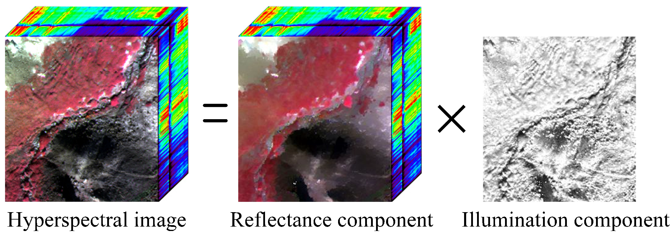
2. Intrinsic Image Decomposition
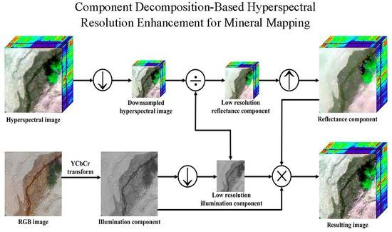
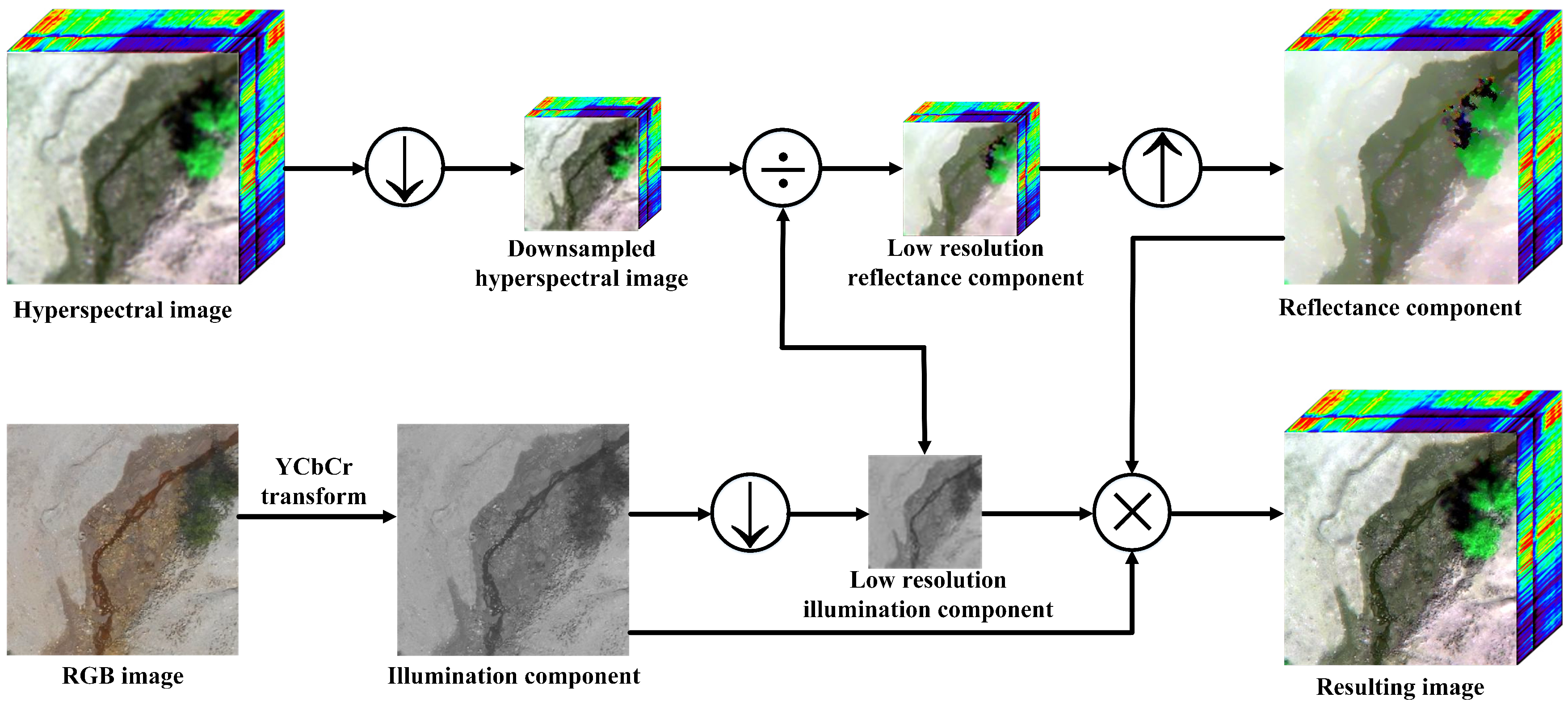
3. Proposed Method
3.1. Estimation of the Illumination Component
3.2. Estimation of the Reflectance Component
3.3. Reconstruction
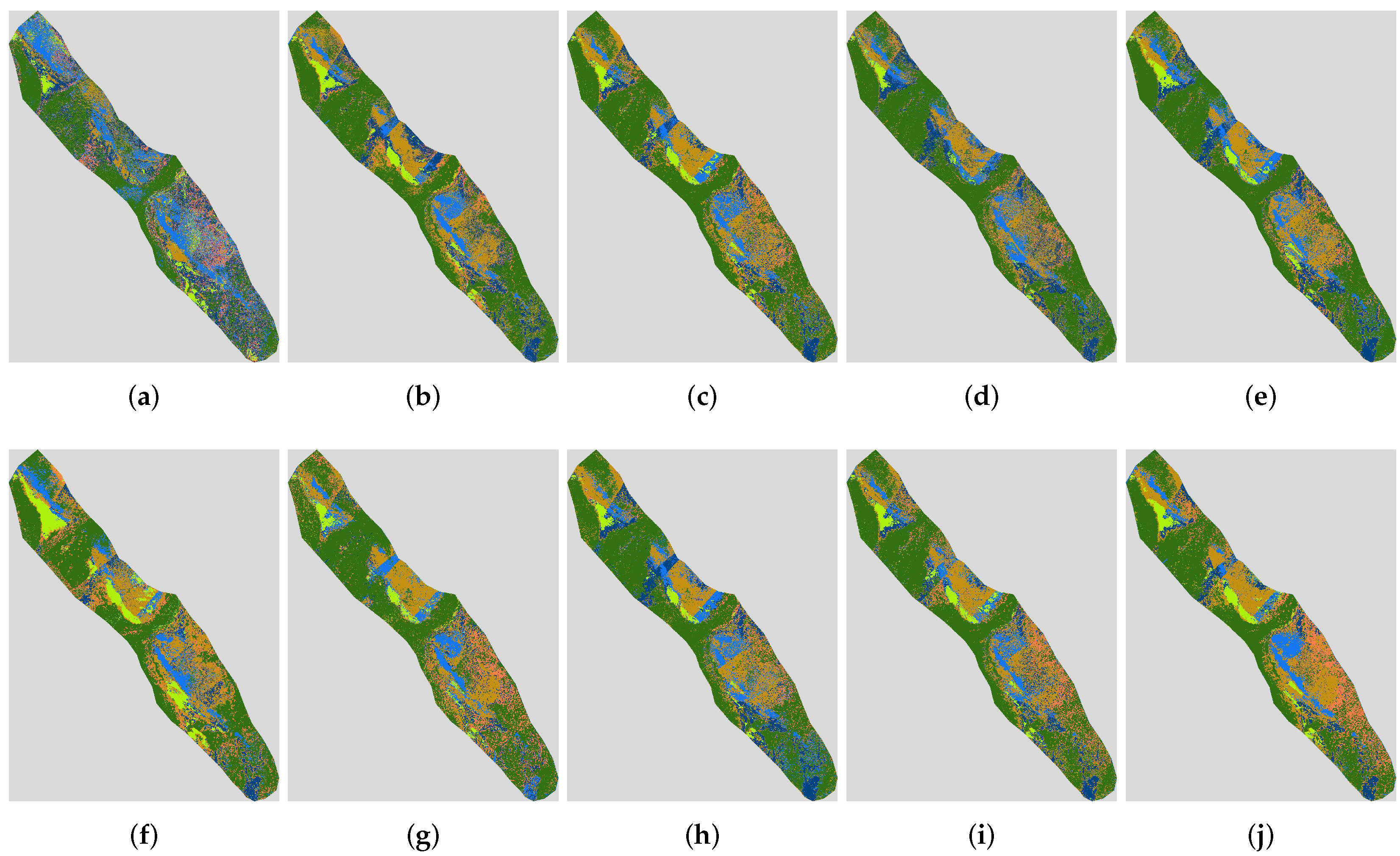
4. Experiments
4.1. Datasets
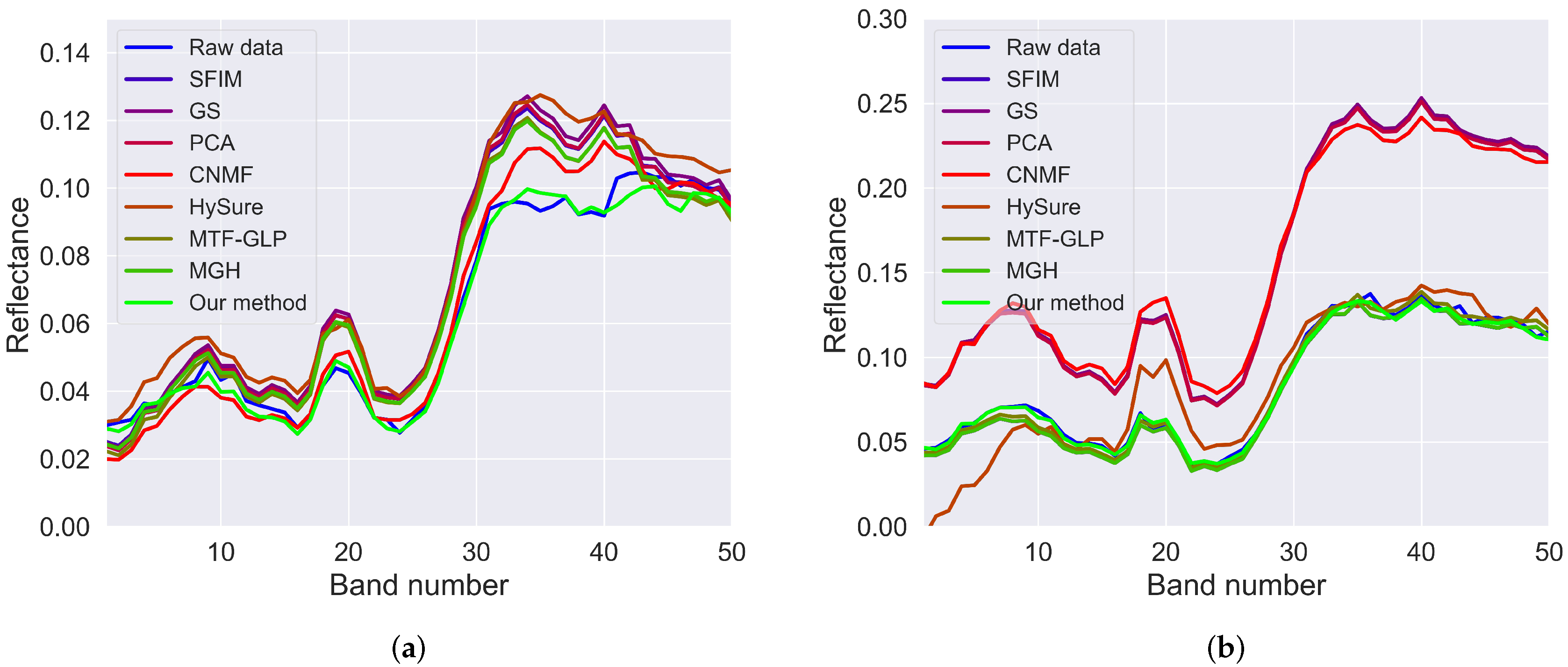
4.2. Quality Indexes
- (1)
- CC: The CC estimates the similar level of the original image and the resulting image:whereHere, X is the reference image, and denotes the fused image. A higher CC indicates the better fusion performance.
- (2)
- SAM: The SAM reflects the spectral quality of the reconstructed result, which is shown as:The SAM is an important index of the spectral distortion of the fused result. A smaller SAM indicates less spectral distortion of the resulting image.
- (3)
- RMSE: The RMSE evaluates the difference between the fused result and the reference data, which is given asThe smaller value indicates better performance. The best value is 1.
- (4)
- ERGAS: The ERGAS assesses the overall quality of the fused result as follows:where c represents the ratio of the spatial resolution between the fused result and the reference data. denotes the mean value of . defines the mean square error between and . The smaller the ERGAS, the better the resulting image is.
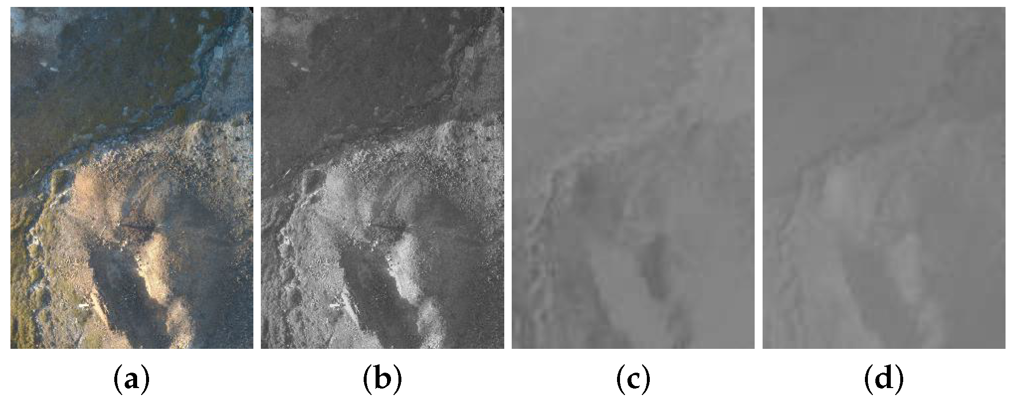
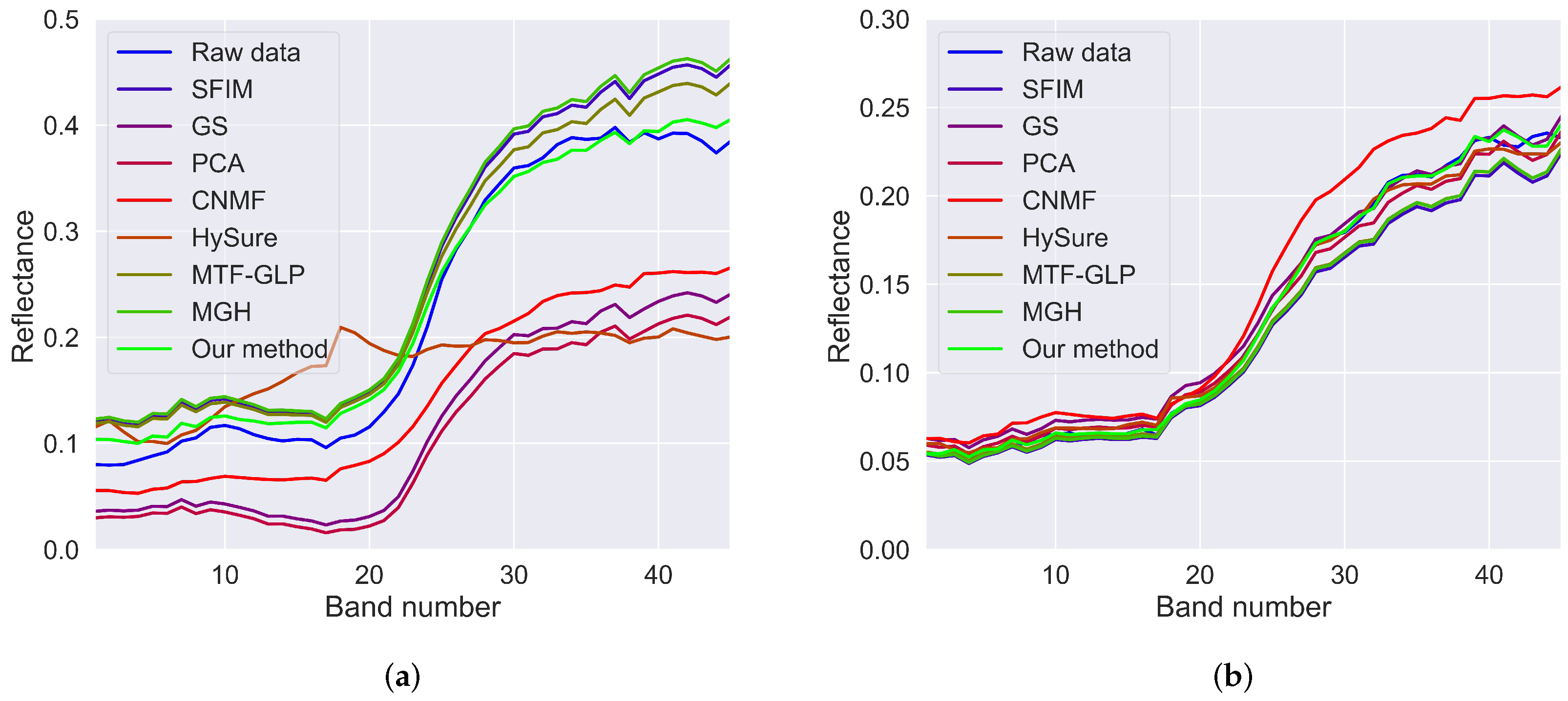
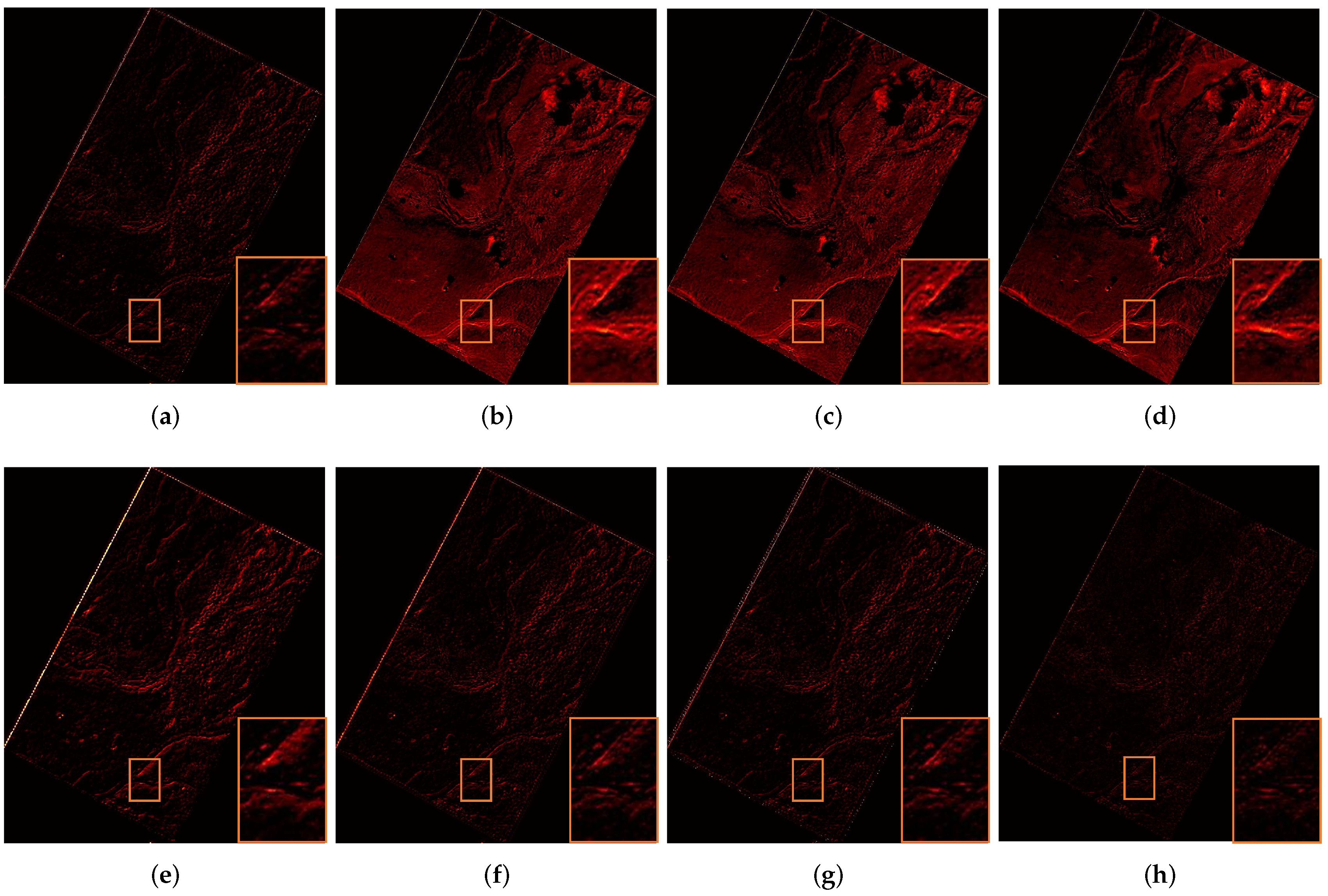
4.3. Resolution Enhancement Results
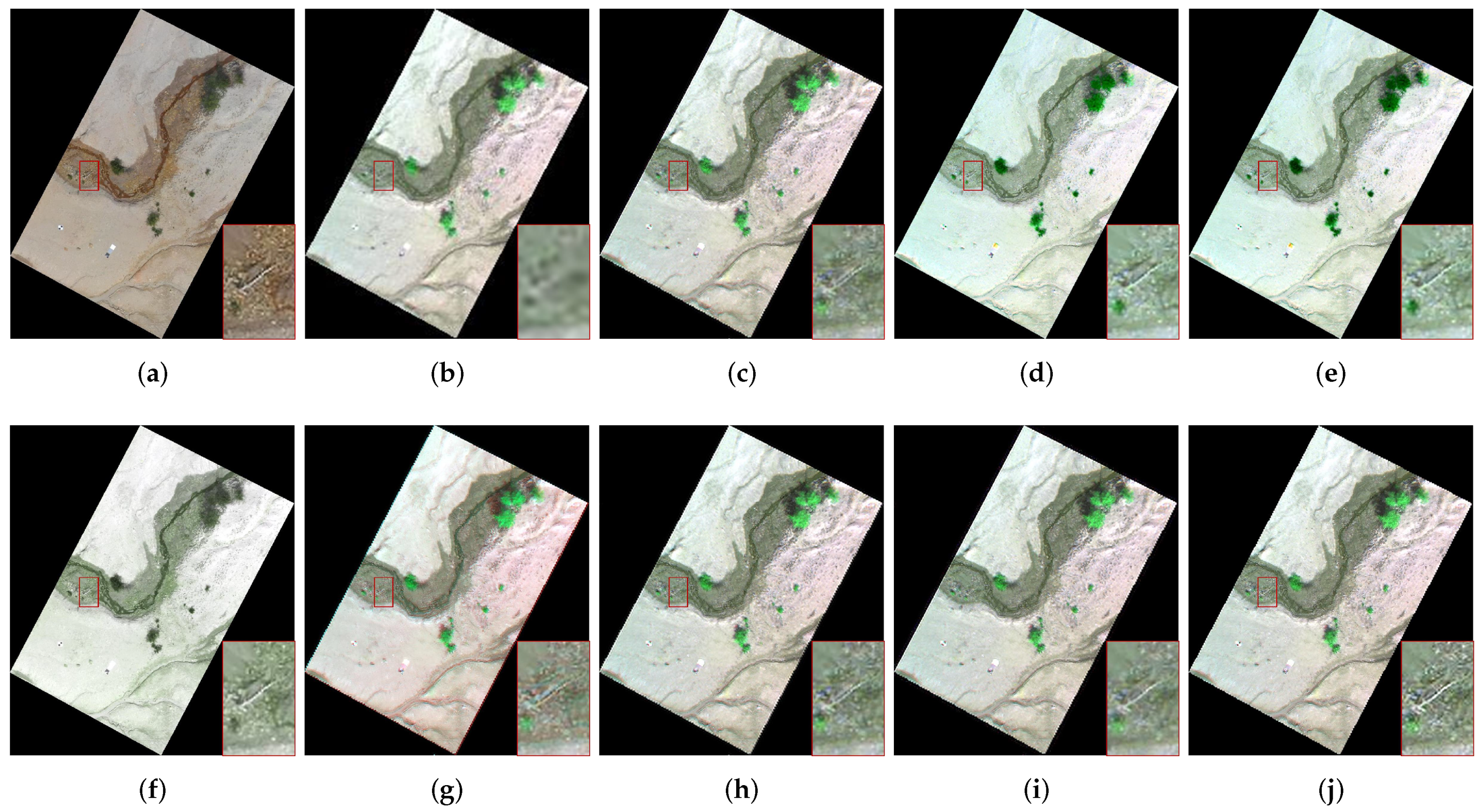
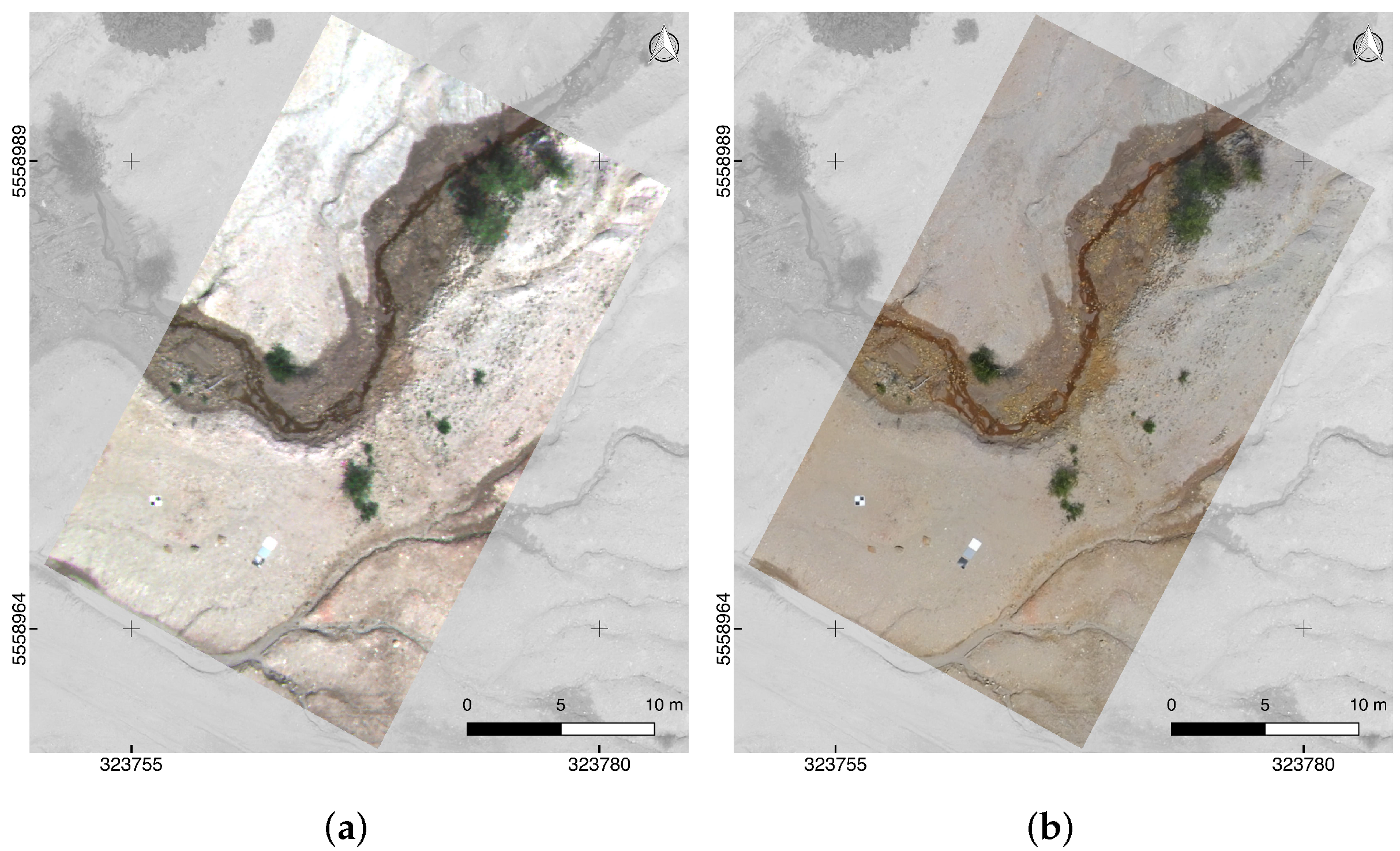
4.3.1. Disko Dataset
4.3.2. Litov Dataset
5. Discussion
5.1. Computing Time
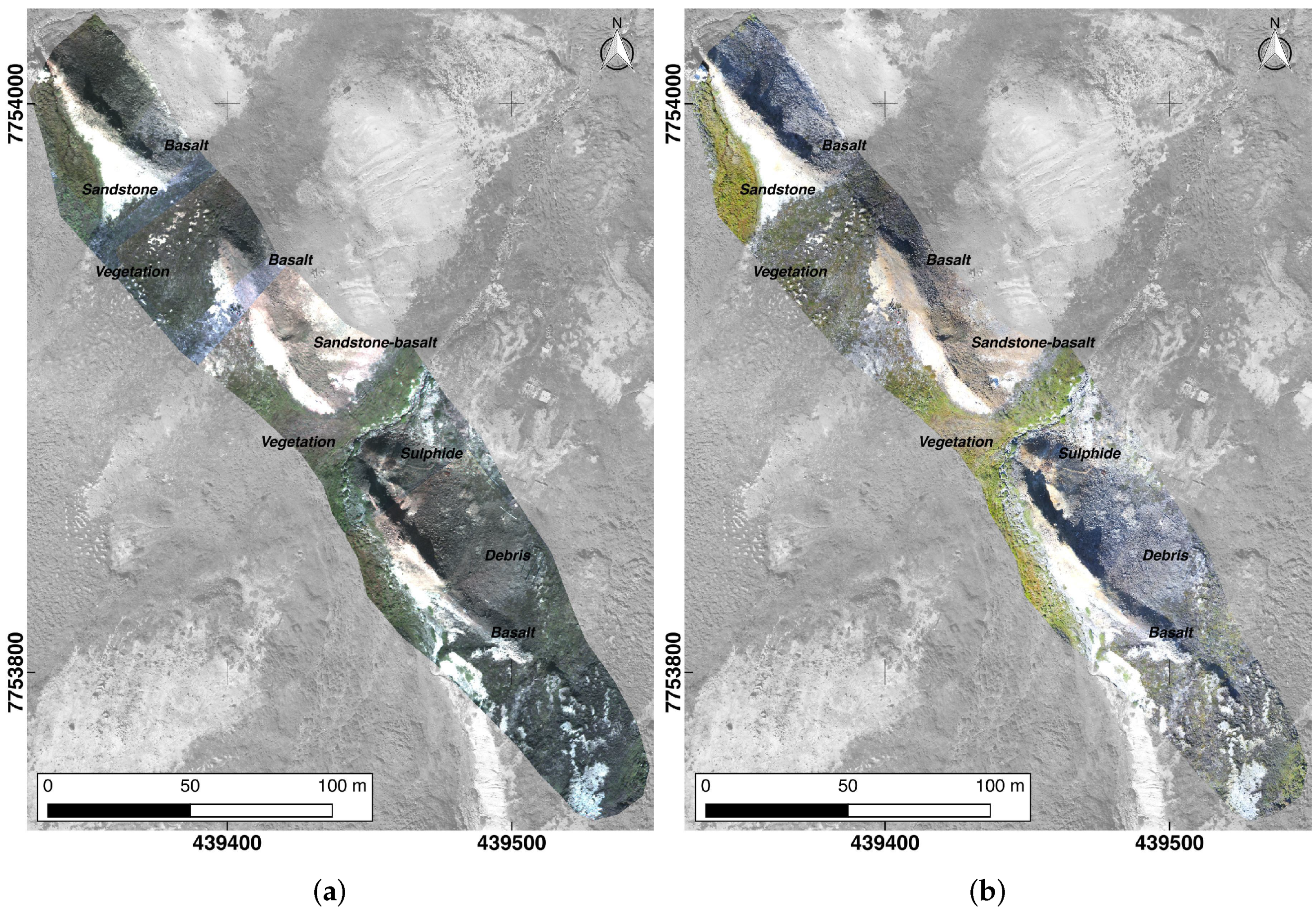
5.2. Mineral Mapping
6. Conclusions
Author Contributions
Funding
Acknowledgments
Conflicts of Interest
References
- Li, H.; Ghamisi, P.; Rasti, B.; Wu, Z.; Shapiro, A.; Schultz, M.; Zipf, A. A Multi-Sensor Fusion Framework Based on Coupled Residual Convolutional Neural Networks. Remote Sens. 2020, 12, 2067. [Google Scholar] [CrossRef]
- Tu, B.; Zhou, C.; Peng, J.; He, W.; Ou, X.; Xu, Z. Kernel Entropy Component Analysis-Based Robust Hyperspectral Image Supervised Classification. Remote Sens. 2019, 11, 2823. [Google Scholar] [CrossRef] [Green Version]
- Duan, P.; Kang, X.; Li, S.; Ghamisi, P. Noise-Robust Hyperspectral Image Classification via Multi-Scale Total Variation. IEEE J. Sel. Top. Appl. Earth Observ. Remote Sens. 2019, 12, 1948–1962. [Google Scholar] [CrossRef]
- Kang, J.; Fernandez-Beltran, R.; Duan, P.; Liu, S.; Plaza, A. Deep Unsupervised Embedding for Remotely Sensed Images based on Spatially Augmented Momentum Contrast. IEEE Trans. Geosci. Remote Sens. 2020. [Google Scholar] [CrossRef]
- Hong, D.; Yokoya, N.; Ge, N.; Chanussot, J.; Zhu, X.X. Learnable manifold alignment (LeMA): A semi-supervised cross-modality learning framework for land cover and land use classification. ISPRS J. Photogramm. Remote Sens. 2019, 147, 193–205. [Google Scholar] [CrossRef]
- Lv, Z.; Liu, T.; Benediktsson, J.A. Object-Oriented Key Point Vector Distance for Binary Land Cover Change Detection Using VHR Remote Sensing Images. IEEE Trans. Geosci. Remote Sens. 2020, 58, 6524–6533. [Google Scholar] [CrossRef]
- Kang, X.; Duan, P.; Xiang, X.; Li, S.; Benediktsson, J.A. Detection and Correction of Mislabeled Training Samples for Hyperspectral Image Classification. IEEE Trans. Geosci. Remote Sens. 2018, 56, 5673–5686. [Google Scholar] [CrossRef]
- Kang, J.; Hong, D.; Liu, J.; Baier, G.; Yokoya, N.; Demir, B. Learning Convolutional Sparse Coding on Complex Domain for Interferometric Phase Restoration. IEEE Trans. Neural Netw. Learn. Syst. 2020, 1–15. [Google Scholar] [CrossRef] [Green Version]
- Hong, D.; Wu, X.; Ghamisi, P.; Chanussot, J.; Yokoya, N.; Zhu, X.X. Invariant Attribute Profiles: A Spatial-Frequency Joint Feature Extractor for Hyperspectral Image Classification. IEEE Trans. Geosci. Remote Sens. 2020, 58, 3791–3808. [Google Scholar] [CrossRef] [Green Version]
- Cecilia Contreras Acosta, I.; Khodadadzadeh, M.; Tusa, L.; Ghamisi, P.; Gloaguen, R. A Machine Learning Framework for Drill-Core Mineral Mapping Using Hyperspectral and High-Resolution Mineralogical Data Fusion. IEEE J. Sel. Top. Appl. Earth Observ. Remote Sens. 2019, 1–14. [Google Scholar]
- Murphy, R.J.; Monteiro, S.T. Mapping the distribution of ferric iron minerals on a vertical mine face using derivative analysis of hyperspectral imagery (430–470 nm). ISPRS J. Photogramm. Remote Sens. 2013, 75, 29–39. [Google Scholar] [CrossRef]
- Hoang, N.T.; Koike, K. Comparison of hyperspectral transformation accuracies of multispectral Landsat TM, ETM+, OLI and EO-1 ALI images for detecting minerals in a geothermal prospect area. ISPRS J. Photogramm. Remote Sens. 2018, 137, 15–28. [Google Scholar] [CrossRef]
- Ghamisi, P.; Rasti, B.; Yokoya, N.; Wang, Q.; Hofle, B.; Bruzzone, L.; Bovolo, F.; Chi, M.; Anders, K.; Gloaguen, R.; et al. Multisource and Multitemporal Data Fusion in Remote Sensing: A Comprehensive Review of the State of the Art. IEEE Geosci. Remote Sens. Mag. 2019, 7, 6–39. [Google Scholar] [CrossRef] [Green Version]
- Lorenz, S.; Seidel, P.; Ghamisi, P.; Zimmermann, R.; Tusa, L.; Khodadadzadeh, M.; Contreras, I.C.; Gloaguen, R. Multi-Sensor Spectral Imaging of Geological Samples: A Data Fusion Approach Using Spatio-Spectral Feature Extraction. Sensors 2019, 19, 2787. [Google Scholar] [CrossRef] [PubMed] [Green Version]
- Gloaguen, R.; Fuchs, M.; Khodadadzadeh, M.; Ghamisi, P.; Kirsch, M.; Booysen, R.; Zimmermann, R.; Lorenz, S. Multi-Source and multi-Scale Imaging-Data Integration to boost Mineral Mapping. In Proceedings of the IGARSS 2019-2019 IEEE International Geoscience and Remote Sensing Symposium, Yokohama, Japan, 28 July 2019; pp. 5587–5589. [Google Scholar] [CrossRef]
- Loncan, L.; de Almeida, L.B.; Bioucas-Dias, J.M.; Briottet, X.; Chanussot, J.; Dobigeon, N.; Fabre, S.; Liao, W.; Licciardi, G.A.; Simões, M.; et al. Hyperspectral Pansharpening: A Review. IEEE Geosci. Remote Sens. Mag. 2015, 3, 27–46. [Google Scholar] [CrossRef] [Green Version]
- De Almeida, C.T.; Galvao, L.S.; de Oliveira Cruz e Aragao, L.E.; Ometto, J.P.H.B.; Jacon, A.D.; de Souza Pereira, F.R.; Sato, L.Y.; Lopes, A.P.; de Alencastro Graca, P.M.L.; de Jesus Silva, C.V.; et al. Combining LiDAR and hyperspectral data for aboveground biomass modeling in the Brazilian Amazon using different regression algorithms. Remote Sens. Environ. 2019, 232, 111323. [Google Scholar] [CrossRef]
- Li, J.; Cui, R.; Li, B.; Song, R.; Li, Y.; Du, Q. Hyperspectral Image Super-Resolution with 1D-2D Attentional Convolutional Neural Network. Remote Sens. 2019, 11, 2859. [Google Scholar] [CrossRef] [Green Version]
- Liu, L.; Coops, N.C.; Aven, N.W.; Pang, Y. Mapping urban tree species using integrated airborne hyperspectral and LiDAR remote sensing data. Remote Sens. Environ. 2017, 200, 170–182. [Google Scholar] [CrossRef]
- Bablet, A.; Viallefont-Robinet, F.; Jacquemoud, S.; Fabre, S.; Briottet, X. High-resolution mapping of in-depth soil moisture content through a laboratory experiment coupling a spectroradiometer and two hyperspectral cameras. Remote Sens. Environ. 2020, 236, 111533. [Google Scholar] [CrossRef]
- He, G.; Zhong, J.; Lei, J.; Li, Y.; Xie, W. Hyperspectral Pansharpening Based on Spectral Constrained Adversarial Autoencoder. Remote Sens. 2019, 11, 2691. [Google Scholar] [CrossRef] [Green Version]
- Hladik, C.; Schalles, J.; Alber, M. Salt marsh elevation and habitat mapping using hyperspectral and LIDAR data. Remote Sens. Environ. 2013, 139, 318–330. [Google Scholar] [CrossRef]
- Tu, T.M.; Su, S.C.; Shyu, H.C.; Huang, P.S. A new look at IHS-like image fusion methods. Inf. Fusion 2001, 2, 177–186. [Google Scholar] [CrossRef]
- Laben, C.A.; Brower, B.V. Process for Enhancing the Spatial Resolution of Multispectral Imagery Using Pan-Sharpening. U.S. Patent 6011875, 4 January 2000. [Google Scholar]
- Liu, J.G. Smoothing Filter-based Intensity Modulation: A spectral preserve image fusion technique for improving spatial details. Int. J. Remote Sens. 2000, 21, 3461–3472. [Google Scholar] [CrossRef]
- Yin, M.; Duan, P.; Liu, W.; Liang, X. A novel infrared and visible image fusion algorithm based on shift-invariant dual-tree complex shearlet transform and sparse representation. Neurocomputing 2017, 226, 182–191. [Google Scholar] [CrossRef]
- He, L.; Zhu, J.; Li, J.; Plaza, A.; Chanussot, J.; Li, B. HyperPNN: Hyperspectral Pansharpening via Spectrally Predictive Convolutional Neural Networks. IEEE J. Sel. Top. Appl. Earth Observ. Remote Sens. 2019, 12, 3092–3100. [Google Scholar] [CrossRef]
- Li, K.; Xie, W.; Du, Q.; Li, Y. DDLPS: Detail-Based Deep Laplacian Pansharpening for Hyperspectral Imagery. IEEE Trans. Geosci. Remote Sens. 2019, 57, 8011–8025. [Google Scholar] [CrossRef]
- Qu, J.; Li, Y.; Dong, W. Hyperspectral Pansharpening With Guided Filter. IEEE Geosci. Remote Sens. Lett. 2017, 14, 2152–2156. [Google Scholar] [CrossRef]
- Qu, J.; Li, Y.; Du, Q.; Dong, W.; Xi, B. Hyperspectral Pansharpening Based on Homomorphic Filtering and Weighted Tensor Matrix. Remote Sens. 2019, 11, 1005. [Google Scholar] [CrossRef] [Green Version]
- Xie, W.; Lei, J.; Cui, Y.; Li, Y.; Du, Q. Hyperspectral Pansharpening With Deep Priors. IEEE Trans. Neural Netw. Learn. Syst. 2019, 31, 1529–1543. [Google Scholar] [CrossRef]
- Dong, W.; Fu, F.; Shi, G.; Cao, X.; Wu, J.; Li, G.; Li, X. Hyperspectral Image Super-Resolution via Non-Negative Structured Sparse Representation. IEEE Trans. Image Process. 2016, 25, 2337–2352. [Google Scholar] [CrossRef]
- Kawakami, R.; Matsushita, Y.; Wright, J.; Ben-Ezra, M.; Tai, Y.; Ikeuchi, K. High-resolution hyperspectral imaging via matrix factorization. In Proceedings of the CVPR 2011, Providence, RI, USA, 20–25 June 2011; pp. 2329–2336. [Google Scholar] [CrossRef]
- Dian, R.; Li, S.; Guo, A.; Fang, L. Deep Hyperspectral Image Sharpening. IEEE Trans. Neural Netw. Learn. Syst. 2018, 29, 5345–5355. [Google Scholar] [CrossRef] [PubMed]
- Zhou, F.; Hang, R.; Liu, Q.; Yuan, X. Pyramid Fully Convolutional Network for Hyperspectral and Multispectral Image Fusion. IEEE J. Sel. Top. Appl. Earth Observ. Remote Sens. 2019, 12, 1549–1558. [Google Scholar] [CrossRef]
- Yokoya, N.; Yairi, T.; Iwasaki, A. Coupled Nonnegative Matrix Factorization Unmixing for Hyperspectral and Multispectral Data Fusion. IEEE Trans. Geosci. Remote Sens. 2012, 50, 528–537. [Google Scholar] [CrossRef]
- Li, S.; Dian, R.; Fang, L.; Bioucas-Dias, J.M. Fusing Hyperspectral and Multispectral Images via Coupled Sparse Tensor Factorization. IEEE Trans. Image Process. 2018, 27, 4118–4130. [Google Scholar] [CrossRef] [PubMed]
- Yang, J.; Zhao, Y.Q.; Chan, J.C.W. Hyperspectral and Multispectral Image Fusion via Deep Two-Branches Convolutional Neural Network. Remote Sens. 2018, 10, 800. [Google Scholar] [CrossRef] [Green Version]
- Shen, L.; Yeo, C.; Hua, B. Intrinsic Image Decomposition Using a Sparse Representation of Reflectance. IEEE Trans. Pattern Anal. Mach. Intell. 2013, 35, 2904–2915. [Google Scholar] [CrossRef]
- Kang, X.; Li, S.; Fang, L.; Benediktsson, J.A. Pansharpening Based on Intrinsic Image Decomposition. Sens. Imag. 2014, 15, 94. [Google Scholar] [CrossRef]
- Yue, H.; Yang, J.; Sun, X.; Wu, F.; Hou, C. Contrast Enhancement Based on Intrinsic Image Decomposition. IEEE Trans. Image Process. 2017, 26, 3981–3994. [Google Scholar] [CrossRef]
- Kang, X.; Li, S.; Fang, L.; Benediktsson, J.A. Intrinsic Image Decomposition for Feature Extraction of Hyperspectral Images. IEEE Trans. Geosci. Remote Sens. 2015, 53, 2241–2253. [Google Scholar] [CrossRef]
- Sheng, B.; Li, P.; Jin, Y.; Tan, P.; Lee, T. Intrinsic Image Decomposition with Step and Drift Shading Separation. IEEE Trans. Vis. Comput. Graph. 2020, 26, 1332–1346. [Google Scholar] [CrossRef]
- Kahu, S.Y.; Raut, R.B.; Bhurchandi, K.M. Review and evaluation of color spaces for image/video compression. Color Res. Appl. 2018, 44, 8–33. [Google Scholar] [CrossRef] [Green Version]
- Vivone, G.; Alparone, L.; Chanussot, J.; Dalla Mura, M.; Garzelli, A.; Licciardi, G.A.; Restaino, R.; Wald, L. A Critical Comparison Among Pansharpening Algorithms. IEEE Trans. Geosci. Remote Sens. 2015, 53, 2565–2586. [Google Scholar] [CrossRef]
- Aiazzi, B.; Alparone, L.; Baronti, S.; Garzelli, A. Context-driven fusion of high spatial and spectral resolution images based on oversampled multiresolution analysis. IEEE Trans. Geosci. Remote Sens. 2002, 40, 2300–2312. [Google Scholar] [CrossRef]
- Vivone, G.; Restaino, R.; Dalla Mura, M.; Licciardi, G.; Chanussot, J. Contrast and Error-Based Fusion Schemes for Multispectral Image Pansharpening. IEEE Geosci. Remote Sens. Lett. 2014, 11, 930–934. [Google Scholar] [CrossRef] [Green Version]
- Simões, M.; Bioucas-Dias, J.; Almeida, L.B.; Chanussot, J. A Convex Formulation for Hyperspectral Image Superresolution via Subspace-Based Regularization. IEEE Trans. Geosci. Remote Sens. 2015, 53, 3373–3388. [Google Scholar] [CrossRef] [Green Version]
- Jakob, S.; Zimmermann, R.; Gloaguen, R. The Need for Accurate Geometric and Radiometric Corrections of Drone-Borne Hyperspectral Data for Mineral Exploration: MEPHySTo-A Toolbox for Pre-Processing Drone-Borne Hyperspectral Data. Remote Sens. 2017, 9, 88. [Google Scholar] [CrossRef] [Green Version]
- Jackisch, R.; Madriz, Y.; Zimmermann, R.; Pirttijärvi, M.; Saartenoja, A.; Heincke, B.; Salmirinne, H.; Kujasalo, J.P.; Andreani, L.; Gloaguen, R. Drone-borne hyperspectral and magnetic data integration: Otanmäki Fe-Ti-V deposit in Finland. Remote Sens. 2019, 11, 2084. [Google Scholar] [CrossRef] [Green Version]
- Jackisch, R.; Lorenz, S.; Zimmermann, R.; Möckel, R.; Gloaguen, R. Drone-Borne Hyperspectral Monitoring of Acid Mine Drainage: An Example from the Sokolov Lignite District. Remote Sens. 2018, 10, 385. [Google Scholar] [CrossRef] [Green Version]
- Zhou, J.; Civco, D.L.; Silander, J.A. A wavelet transform method to merge Landsat TM and SPOT panchromatic data. Int. J. Remote Sens. 1998, 19, 743–757. [Google Scholar] [CrossRef]
- Zeng, Y.; Huang, W.; Liu, M.; Zhang, H.; Zou, B. Fusion of satellite images in urban area: Assessing the quality of resulting images. Int. Conf. Geoinform. 2010, 1–4. [Google Scholar] [CrossRef]
- Melgani, F.; Bruzzone, L. Classification of hyperspectral remote sensing images with support vector machines. IEEE Trans. Geosci. Remote Sens. 2004, 42, 1778–1790. [Google Scholar] [CrossRef] [Green Version]
- Duan, P.; Kang, X.; Li, S.; Ghamisi, P. Multichannel Pulse-Coupled Neural Network-Based Hyperspectral Image Visualization. IEEE Trans. Geosci. Remote Sens. 2019, 1–13. [Google Scholar] [CrossRef]
- Duan, P.; Kang, X.; Li, S.; Ghamisi, P.; Benediktsson, J.A. Fusion of Multiple Edge-Preserving Operations for Hyperspectral Image Classification. IEEE Trans. Geosci. Remote Sens. 2019, 57, 10336–10349. [Google Scholar] [CrossRef]
- Zhao, J.; Zhong, Y.; Hu, X.; Wei, L.; Zhang, L. A robust spectral-spatial approach to identifying heterogeneous crops using remote sensing imagery with high spectral and spatial resolutions. Remote Sens. Environ. 2020, 239, 111605. [Google Scholar] [CrossRef]
- Dalponte, M.; Bruzzone, L.; Vescovo, L.; Gianelle, D. The role of spectral resolution and classifier complexity in the analysis of hyperspectral images of forest areas. Remote Sens. Environ. 2009, 113, 2345–2355. [Google Scholar] [CrossRef]
- Kang, X.; Duan, P.; Li, S. Hyperspectral image visualization with edge-preserving filtering and principal component analysis. Inf. Fusion 2020, 57, 130–143. [Google Scholar] [CrossRef]
- Duan, P.; Lai, J.; Kang, J.; Kang, X.; Ghamisi, P.; Li, S. Texture-aware total variation-based removal of sun glint in hyperspectral images. ISPRS J. Photogramm. Remote Sens. 2020, 166, 359–372. [Google Scholar] [CrossRef]


| Indexes | Best | SFIM | GS | PCA | CNMF | HySure | MTF_GLP | MGH | Our Method |
|---|---|---|---|---|---|---|---|---|---|
| CC | 1 | 0.957 | 0.937 | 0.932 | 0.962 | 0.948 | 0.963 | 0.932 | 0.967 |
| SAM | 0 | 1.032 | 1.487 | 1.707 | 1.469 | 3.261 | 1.121 | 1.071 | 0.744 |
| RMSE | 0 | 0.029 | 0.034 | 0.035 | 0.023 | 0.031 | 0.024 | 0.074 | 0.023 |
| ERGAS | 0 | 12.003 | 12.707 | 13.179 | 8.358 | 11.334 | 8.621 | 37.466 | 8.061 |
| Indexes | Best | SFIM | GS | PCA | CNMF | HySure | MTF_GLP | MGH | Our Method |
|---|---|---|---|---|---|---|---|---|---|
| CC | 1 | 0.831 | 0.985 | 0.983 | 0.983 | 0.973 | 0.986 | 0.705 | 0.994 |
| SAM | 0 | 1.982 | 2.332 | 2.422 | 2.031 | 3.376 | 1.831 | 1.980 | 1.056 |
| RMSE | 0 | 0.175 | 0.017 | 0.018 | 0.019 | 0.023 | 0.016 | 0.330 | 0.010 |
| ERGAS | 0 | 68.56 | 4.394 | 4.613 | 4.474 | 6.145 | 4.201 | 115.312 | 2.664 |
| Datasets | SFIM | GS | PCA | CNMF | HySure | MTF_GLP | MGH | Our Method |
|---|---|---|---|---|---|---|---|---|
| Best value | 0 | 0 | 0 | 0 | 0 | 0 | 0 | 0 |
| Disko | 36.81 | 28.06 | 27.55 | 168.05 | 2068.51 | 54.19 | 44.74 | 6.64 |
| Litov | 14.23 | 13.47 | 13.12 | 75.01 | 883.64 | 15.37 | 14.78 | 4.57 |
| Classes | Name | Train | Test |
|---|---|---|---|
| 1 | Vegetation | 55 | 104 |
| 2 | Sandstone | 104 | 62 |
| 3 | Basalt | 72 | 46 |
| 4 | Sulphide | 105 | 157 |
| 5 | Debris | 56 | 68 |
| 6 | Sandstone-basalt | 91 | 40 |
| Total | 483 | 477 | |
| Class | RGB | HSI | SFIM | GS | PCA | CNMF | HySure | MTF_GLP | MGH | Our Method |
|---|---|---|---|---|---|---|---|---|---|---|
| 1 | 78.79 | 90.00 | 82.35 | 97.12 | 79.49 | 88.18 | 53.76 | 87.16 | 79.67 | 79.69 |
| 2 | 50.98 | 91.18 | 98.41 | 93.65 | 100.0 | 67.39 | 96.49 | 100.0 | 96.88 | 96.88 |
| 3 | 19.54 | 26.04 | 32.74 | 24.22 | 20.81 | 18.82 | 35.71 | 19.43 | 27.78 | 32.54 |
| 4 | 69.52 | 78.95 | 69.70 | 79.31 | 30.30 | 57.14 | 85.96 | 18.52 | 63.16 | 87.04 |
| 5 | 38.46 | 84.62 | 42.50 | 75.86 | 50.00 | 55.56 | 44.83 | 53.33 | 57.78 | 72.50 |
| 6 | 31.03 | 30.56 | 50.00 | 38.46 | 54.05 | 39.47 | 44.44 | 54.05 | 58.06 | 55.38 |
| OA | 51.99 | 53.46 | 62.47 | 58.49 | 52.2 | 49.90 | 57.23 | 52.83 | 61.43 | 66.46 |
| AA | 48.05 | 66.89 | 62.62 | 68.10 | 55.78 | 54.43 | 60.20 | 55.42 | 63.89 | 70.67 |
| Kappa | 41.38 | 46.23 | 55.04 | 51.62 | 43.99 | 40.96 | 48.26 | 44.98 | 53.92 | 59.97 |
© 2020 by the authors. Licensee MDPI, Basel, Switzerland. This article is an open access article distributed under the terms and conditions of the Creative Commons Attribution (CC BY) license (http://creativecommons.org/licenses/by/4.0/).
Share and Cite
Duan, P.; Lai, J.; Ghamisi, P.; Kang, X.; Jackisch, R.; Kang, J.; Gloaguen, R. Component Decomposition-Based Hyperspectral Resolution Enhancement for Mineral Mapping. Remote Sens. 2020, 12, 2903. https://0-doi-org.brum.beds.ac.uk/10.3390/rs12182903
Duan P, Lai J, Ghamisi P, Kang X, Jackisch R, Kang J, Gloaguen R. Component Decomposition-Based Hyperspectral Resolution Enhancement for Mineral Mapping. Remote Sensing. 2020; 12(18):2903. https://0-doi-org.brum.beds.ac.uk/10.3390/rs12182903
Chicago/Turabian StyleDuan, Puhong, Jibao Lai, Pedram Ghamisi, Xudong Kang, Robert Jackisch, Jian Kang, and Richard Gloaguen. 2020. "Component Decomposition-Based Hyperspectral Resolution Enhancement for Mineral Mapping" Remote Sensing 12, no. 18: 2903. https://0-doi-org.brum.beds.ac.uk/10.3390/rs12182903