A 117 Line 2D Digital Image Correlation Code Written in MATLAB


Department of Mechanical and Mechatronic Engineering, Stellenbosch University, Corner of Banghoek and Joubert Street, Stellenbosch, Western Cape 7599, South Africa
*
Author to whom correspondence should be addressed.
Remote Sens. 2020, 12(18), 2906; https://0-doi-org.brum.beds.ac.uk/10.3390/rs12182906
Submission received: 22 July 2020
/
Revised: 2 September 2020
/
Accepted: 3 September 2020
/
Published: 8 September 2020
(This article belongs to the Special Issue Digital Image Processing)
Abstract
:Digital Image Correlation (DIC) has become a popular tool in many fields to determine the displacements and deformations experienced by an object from images captured of the object. Although there are several publications which explain DIC in its entirety while still catering to newcomers to the concept, these publications neglect to discuss how the theory presented is implemented in practice. This gap in literature, which this paper aims to address, makes it difficult to gain a working knowledge of DIC, which is necessary in order to contribute towards its development. The paper attempts to address this by presenting the theory of a 2D, subset-based DIC framework that is predominantly consistent with state-of-the-art techniques, and discussing its implementation as a modular MATLAB code. The correlation aspect of this code is validated, showing that it performs on par with well-established DIC algorithms and thus is sufficiently reliable for practical use. This paper, therefore, serves as an educational resource to bridge the gap between the theory of DIC and its practical implementation. Furthermore, although the code is designed as an educational resource, its validation combined with its modularity makes it attractive as a starting point to develop the capabilities of DIC.
1. Introduction
Digital image correlation (DIC) determines the displacements and deformations at multiple points spanning the surface of an object (full-field displacements and deformations) from images captured of the object. It is type of a full-field, non-contact optical technique and these techniques are categorised as either interferometric or non-interferometric. The interferometric techniques, such as Electronic Speckle Pattern Interferometry and Moiré Interferometry, require a coherent light source and need to be isolated from vibrations [1]. As such, their utilisation is in the confines of a laboratory. In contrast, non-interferometric techniques, DIC and the grid method require simple incoherent light and are more robust with regards to ambient vibrations and light variations [2]. Thus, non-interferometric techniques are more attractive due to their less stringent requirements and are mostly used in open literature. DIC allows for a more straightforward setup compared to the grid method as it only requires a random, irregular pattern on the surface of the object instead of a regular grid.
These advantages of DIC over other full-field, non-contact optical techniques, along with the decreasing cost and increasing performance of digital cameras, has led to widespread use of DIC in various fields. Some applications of DIC include: (i) performing human pulse monitoring [3,4]; (ii) analysing the stick-slip behaviour of tyre tread [5]; (iii) determining the mechanical properties of biological tissue [6,7,8]; (iv) in situ health monitoring of structures and components [9,10,11]; (v) analysing vibration of components [12,13]; and (vi) remote sensing applications [14,15,16,17]. However, DIC has received the most attention, and thus development, for applications in experimental solid mechanics. As such, this paper will predominantly focus on DIC in the context of experimental solid mechanics applications.
In the field of experimental solid mechanics, measuring the displacement and deformation experienced by a specimen, as a result of an applied load, is essential to quantify its mechanical properties. As such, DIC is advantageous for three reasons: Firstly, its full-field nature allows more complex constitutive equations to be used to determine more than one material property at a time, using methods such as the virtual fields method [18,19,20] and the finite element model updating method [21]. Secondly, the non-contact nature of DIC avoids altering mechanical properties of the materials being tested, such as in the case of determining the material properties of biological tissue [6,7,8] and hyper-elastic materials [22]. Lastly, DIC allows the specimen to be exposed to harsh environments, such as high-temperature applications, while still being able to take measurements, provided the specimen is visible [23].
When DIC was first introduced by Peters and Ranson in 1982 [24], it used a simple cross-correlation criterion with a zero-order shape function (SF) and could not account for the deformation of the specimen or variations in ambient light. Between 1983 and 1989, Sutton and his colleagues improved the technique by introducing the first-order SF [25], the normalised cross-correlation criterion which is more robust against light variations [26], the Newton–Raphson (NR) optimisation method [27] and bi-cubic b-spline interpolation [28]. The two-dimensional (2D) DIC technique was extended to three dimensions (3D or stereovision DIC) in 1993 by Luo et al. [29] and to digital volume correlation (DVC) in 1999 by Bay et al. [30] using X-Ray tomography-computed images.
The most significant contributions to the current state-of-the-art DIC technique, as identified by Pan [2], occurred during the 21st century. In 2000, Schreier et al. [31] proved that bi-quintic b-spline interpolation is the best interpolation method for accurate sub-pixel displacements. In the same year, Lu and Cary [32] introduced the second-order SF to account for more complex deformations. In 2004, Baker and Matthews [33] proposed the inverse compositional Gauss–Newton (IC-GN) optimisation method using the sum of squared difference correlation criterion which is more efficient than the NR method. However, Tong showed in 2005 [34] that the zero-mean normalised sum of squared difference (ZNSSD) correlation criterion is the most reliable and so Pan et al. [35] adapted the IC-GN method to use the ZNSSD criterion in 2013. Finally, Gao et al. [36] introduced the second-order SF to the IC-GN method in 2015. The IC-GN method is considered to be the state-of-the-art optimisation method because it has been shown to be theoretically equivalent to the NR method [33] while offering improved accuracy, robustness to noise and computational efficiency in practice [37].
The DIC process is complicated, comprising of several intricate elements, including correlation, camera calibration, transformation of displacements between the device and real-world coordinates and strain computation. Successful application of DIC requires an understanding of all these elements and thus newcomers to the field need to overcome a difficult learning curve. To this end, there are several papers which give a comprehensive breakdown of the theory involved in the DIC process, such as the papers by Pan et al. [35], Gao et al. [36] and Blaber et al. [38]. However, in order to contribute towards the development of DIC, a deep understanding of the DIC process and its elements is required. It is incredibly time-consuming to gain this working knowledge due to a lack of publications that directly bridge the gap between the theory and its implementation in code. More specifically, papers either do not provide code that details the implementation of the theory in practice [35,36] or the code that they provide is too complex to be beneficial as a learning resource [38].
This paper aims to bridge the gap between the theory and implementation of DIC. It does this by firstly presenting the theory for a 2D, subset based DIC framework that is predominantly consistent with current state-of-the-art practices. Thereafter the implementation of the theory of the framework as the provided 117 line MATLAB code is discussed. Lastly the correlation aspect of the code is validated using the DIC Challenge image sets documented by Reu et al. [39]. More specifically, its results are discussed in parallel with those obtained using either the commercial software package by LaVision (Davis) and the open-source software Ncorr [38] or, to results documented in the DIC Challenge paper [39], in order to draw conclusions.
The framework, referred to as the ADIC2D framework, is implemented using MATLAB because its simple syntax does not distract the reader from the mathematics of the code. Additionally, its built-in functions are used to simplify the code and improve its efficiency. The code is modular, allowing readers to progressively build up their understanding of the code so that recognising the connection between the theory and code is straightforward. Moreover, this modularity allows for rapid adaption of the code thereby encouraging readers to develop the capabilities of DIC.
2. Framework Theory
DIC consists of four processes: calibration, correlation, displacement transformation and strain computation. Calibration involves determining the parameters of the camera model which relates the location of a point on an object in the real world to the location of the corresponding point in an image taken of the object. Correlation calculates how portions of the object, captured in the image set, displace throughout the image set. Displacement transformation then uses the parameters determined by calibration to transform the pixel displacements determined by correlation to metric displacements in the real world. Finally strain computation determines the strain fields experienced by the specimen from the displacement fields.
2.1. Calibration
Calibration determines the parameters of the camera model. ADIC2D uses the pinhole camera model to transform the location of a point in the real world to the idealised location of the point in the image. Then, a radial distortion model is used to relate the idealised location of this point to its actual distorted location, as illustrated in Figure 1.
2.1.1. Homogeneous Coordinates
The pinhole camera model works with homogeneous coordinates as these allow rotation, translation, scaling and perspective projection to be applied using matrix multiplication. An -element vector, which represents a point in -dimensional space, is converted to homogeneous coordinates by appending a scaling variable of unity to the end of the vector. Converting back from homogeneous coordinates involves dividing each element of the vector by the last element, the scaling variable, before removing the last element. Homogeneous coordinate vectors are indicated by underlining the variable name. For more information on homogeneous coordinates, refer to the work of Bloomenthal and Rokne [40].
2.1.2. Pinhole Camera Model
The pinhole camera model relates the location of a point in the world coordinate system (CS) to its corresponding idealised location in the sensor CS. The 3D world CS is defined such that its x-y plane is coincident with the surface of the specimen under consideration: 2D DIC is limited to determining displacements that occur within this x-y plane. The 2D sensor CS is defined such that its x-y plane is coincident with the plane of the charge-coupled device which captures light rays incident upon its surface as an image.
Let the homogeneous coordinates in the world and sensor CS be and , respectively. Note that the circumflex indicates that the coordinates are ideal (undistorted). The pinhole camera model is given as [41]:
where matrices and contain the extrinsic and intrinsic camera parameters respectively. The extrinsic camera parameters define a rotation matrix and a translation vector which define the position and orientation of the world CS relative to the position and orientation of the camera. Thus, the extrinsic camera parameters change if the relative position or orientation between the specimen and camera change.
In contrast, the intrinsic camera parameters remain unchanged because they are only dependent on the camera system. The parameters and perform scaling from metric units to units of pixels. This paper uses millimetres as the metric units. The parameters and apply translation such that the origin of the sensor CS is at the top left of the image as shown in Figure 1. The parameter converts from an orthogonal CS to a skewed sensor CS. Here, since an orthogonal sensor CS is assumed. The parameter is an arbitrary scaling variable of the homogeneous coordinates which is factored out. For more information on the pinhole camera model refer to the work of Zhang [41] and Heikkila et al. [42].
2.1.3. Radial Distortion Model
According to Tsai [43] and Wei et al. [44], the difference between the ideal and actual image can be well accounted for by using only a radial distortion model. Radial distortion is caused by the lens system having different magnification levels depending on where the light ray passes through the lenses. The image experiences either an increase (pincushion distortion) or decrease (barrel distortion) in magnification with increasing distance from the optical axis. The radial distortion model requires that be converted to normalised ideal image coordinates, , using the inverse of the intrinsic parameter matrix as
This equation includes a matrix to convert from homogeneous coordinates to Cartesian coordinates. is related to the normalised, distorted image coordinates, , as [41]
where and are the unit-less radial distortion parameters that quantify the severity of the distortion. is converted to distorted coordinates in the distorted sensor CS, , as
2.1.4. Calibration Process
Calibration determines the extrinsic, intrinsic and radial distortion parameters using images taken of a calibration plate. A calibration plate is an object with a flat surface having a high contrast regular pattern which contains distinctive, point-like features called calibration targets (CTs). It is used to define a set of 3D coordinates in the world CS and a corresponding set of distorted, 2D coordinates in the distorted sensor CS.
The 3D coordinates of these CTs in the world CS are predefined. In fact, they lie on the x-y plane of the world CS and define its position and orientation. The set of corresponding distorted, 2D coordinates in the sensor CS can be determined by locating the CTs in an image taken of the calibration plate. These two sets of 3D and 2D coordinates are used to solve for the parameters of the camera model, which describe the relationship between the two. This is done in two steps.
The first step determines initial estimates for the extrinsic and intrinsic camera parameters using the closed form solution method proposed by Zhang [41]. The initial estimate of the radial distortion parameters is set to zero.
The second step works with two sets of CTs in the distorted sensor CS: the true CTs, , obtained directly from the calibration images and the calculated CTs, , obtained by transforming the known CTs of the world CS to the distorted sensor CS using the camera model and the current estimate of the calibration parameters. The difference between the true and calculated CTs is quantified as the total projection error, , given as
There are many calibration images and many CTs per calibration image. The second step uses iterative non-linear least-squares optimisation to solve for the calibration parameters which minimise . Note that multiple calibration images are used in order to form an over-determined system of equations. This makes the calibration process less sensitive to noise inherent in the images. For more information on the calibration process refer to the work of Zhang [41] and Heikkila et al. [42].
The last process in calibration corrects for the thickness of the calibration plate, , such that the x-y plane of the world CS is coincident with the surface of the specimen under consideration. The corrected translation vector, , that replaces in Equation (1) is determined as
where and are the translation vector and rotation matrix determined by the above calibration process.
2.2. Correlation
Correlation considers two images: a reference image, , representing the specimen at time , and a deformed image, , representing the specimen at time . is broken up into subsets which are groups of neighbouring pixels. Conceptually, correlation attempts to determine how a reference subset () must displace and deform such that it matches a corresponding subset, the investigated subset () in . In practice, however, remains unchanged while its pixel centre positions (hereafter referred to as pixel positions) are displaced and deformed according to , a predefined SF, resulting in the query points of the investigated subset. The investigated subset is obtained by sampling the deformed image at these query points. To better understand this, some details of correlation need to be explained.
Correlation operates in the distorted sensor CS, as illustrated in Figure 2. ’s centre position, , has been displaced by and in the x- and y-direction, respectively, to obtain ’s centre position, . The th pixel position of , given by , is based on and the distance from to , , as
Similarly, the corresponding th query point of , , is based on and the distance from to , , as
is defined relative to because is unknown prior to correlation. and are a special case of and for the pixel at the centre of the investigated subset. is determined using which modifies according to a given displacement and deformation quantified by the shape function parameters (SFPs), , as
Each pixel of the investigated subset, , is populated by sampling the light intensity of the deformed image at . However, images are discrete and so interpolation must be used to obtain these light intensities of at non-integer locations. As such, and are treated as functions which return the light intensity at a location in the image. For this involves interpolation. The pixels of and are populated by sampling these functions as
The similarity between and is quantified by the correlation criterion. Correlation aims to find the SFPs which define an investigated subset which closely matches the reference subset.
2.2.1. Correlation Criterion
The two most popular types are the ZNSSD and zero-mean normalised cross-correlation (ZNCC) criteria, which are robust against offset and scaling changes in light intensity. The ZNSSD criterion, which has a range of , where 0 indicates a perfect match, is calculated as
where is the number of pixels contained within a subset, and are the mean light intensity values, and and are the normalisation functions of subsets and , respectively. Similarly, the ZNCC criterion, which has a range of , where 1 indicates a perfect match, is given as
Pan et al. [45] proved that these two criteria are related as
The more computationally efficient ZNSSD criterion is evaluated within ADIC2D; however, it is reported as the ZNCC coefficient, using Equation (13), because its range is more intuitive. For more information on correlation criteria refer to the work of Pan et al. [45].
2.2.2. Shape Function
The most common SFs are the zero (), first () and second-order SFs () expressed as [32]
where and represent the displacement of in the x- and y-directions respectively, and their derivatives (subscript and ) define the deformation with respect to the reference subset. Specifically, , , and represent elongation while , , , , and represent shearing of the subset. Higher order SFs, containing higher order displacement derivatives, allow for more complex deformation as shown in Figure 3.
This enables higher order SFs to more reliably track subsets in complex displacement fields. The elements of , for each SF order, are stored as
2.2.3. Interpolation
Interpolation determines the value at a query point () in an image by fitting an equation to the surrounding light intensity data and evaluating the equation at . Polynomial interpolation and b-spline interpolation, shown in Figure 4 for the one-dimensional case, are the most popular types for DIC.
Polynomial interpolation fits a local polynomial equation of order to a window of data of size as shown in grey in Figure 4b for cubic polynomial interpolation. The resulting interpolation equation is a piecewise polynomial where only the central portion of each local polynomial equation is used. The interpolation equation is C0 and C1 continuous for linear and cubic polynomial interpolation, respectively. Refer to the work of Keys [46] for more information on cubic polynomial interpolation.
In contrast, b-spline interpolation builds up an interpolation equation from locally supported basis functions. More specifically, a basis function is defined at each data point and the coefficients of all these basis functions are determined simultaneously from the data. This is done such that the summation of the basis functions forms the interpolation equation as shown in Figure 4c. For cubic b-spline, the interpolation equation is C2 continuous. Refer to the work of Hou et al. [47] for an in-depth discussion of bi-cubic b-spline interpolation.
The interpolation method should be as exact as possible in order for correlation to determine sub-pixel displacements reliably and efficiently because interpolation is the most time consuming part of correlation for iterative, sub-pixel DIC [48].
2.2.4. Gaussian Filtering
High order interpolation methods, such as bi-cubic b-spline interpolation, are sensitive to high frequency noise contained in the images [49]. A Gaussian low-pass filter is used to attenuate the high frequency noise of each image of the image set in order to reduce the bias of the displacement results caused by the interpolation method. Gaussian filtering convolves a 2D Gaussian point-spread function with the image. The Gaussian function consists of a window size, (in pixels), and standard deviation, , to determine a weighted average light intensity at each pixel position in the filtered image from a window of pixels in the unfiltered image. The Gaussian point-spread function is scaled such that the sum of itself equals 1.
Although interpolation is only required for , all the images of the image set (including ) need to be filtered such that the light intensity patterns of the subsets, considered by the correlation criterion, are directly comparable. Despite the fact that variance of the displacement results is independent of the interpolation method, it is dependent on the image detail which is reduced by smoothing [50]. Therefore and should be chosen to reduce bias while not significantly increasing variance. For more information on Gaussian filtering refer to Pan’s work [49].
2.2.5. Optimisation Method
The optimisation problem aims to minimise the correlation criterion (Equation (11)) by using the IC-GN method to iteratively solve for the optimal SFPs. An illustration of this process is shown in Figure 5. Substituting Equation (10) into Equation (11) results in an expression in terms of and being obtained. In addition, Equation (11) is modified to include an iterative improvement estimate, . Normally, iterative updating uses the forward additive implementation in which both and are applied to the investigated subset as . However, for the inverse compositional implementation is applied to the reference subset and the current estimate of is applied to the investigated subset. Thus, the objective function is given as
Taking the first-order Taylor series expansion of Equation (16) in terms of gives
where is the light intensity gradient of and is the Jacobian of the SF at each pixel position. For the zero, first and second-order SFs is given as [32,33]
Setting Equation (17) to zero and taking the derivative with respect to gives the first-order, least-squares solution. Rearranging to make the subject of the equation yields
where is the Hessian given by Equation (20) and the remaining terms, within the summation, of Equation (19) form the Jacobian, . is independent of the SFPs and remains constant during iterations. Thus, Equation (20) can be pre-computed before iterations begin.
Note that since is applied to the reference subset, each iteration solves for a set of SFPs which if applied to the reference subset would improve the correlation criterion. However, instead of applying to the reference subset it is used to improve the estimate of the SFPs of the investigated subset. More specifically, the updated SFPs of the investigated subset, , are obtained by composing the inverted iterative improvement, , with the current estimate, , as
where is a function which populates a square matrix with the values of the SFPs as [36]
where through are
| , | , |
| , | , |
| , | , |
| , | , |
| , | , |
| , | , |
| , | , |
| , | , |
| and . |
The optimisation method is computationally efficient because before iterations begin the following are computed: (i) and its inverse; (ii) the interpolation coefficients of ; and (iii) the image gradients of using the Prewitt gradient operator. Each iteration step involves evaluating (Equation (14)) using the current estimate of to obtain , which is used by Equation (8) to compute , interpolating at in order to compute , and and finally computing using Equation (19). For each iteration is updated using Equation (21). Iterations continue until the stopping criterion deems that is a solution. The correlation coefficient is then computed using Equation (11) substituted into Equation (13) and and are obtained from the SFPs.
2.2.6. Stopping Criterion
2.3. Displacement Transformation
Displacement transformation maps and from the distorted sensor CS to the world CS. First, the position of the investigated subset, , is determined as
An exact analytical solution for the inverse of Equation (3) does not exist because it requires determining the roots of a polynomial of degree greater than four [51]. As such distortion is removed from the reference and investigated subset positions using non-linear, least-squares optimisation.
The resulting undistorted sensor coordinates of the subset before, , and after deformation, , are transformed to the world CS using the inverse of the pinhole camera model as
The corrected translation vector determined by Equation (6) is used in Equation (25). The resulting position of the reference, , and investigated subsets, , in the world CS are used to determine the metric displacement experienced by the subset, , as
2.4. Strain Computation
Strains are computed from the gradients of the displacements determined using Equation (26). A method of smoothing displacements before differentiation is recommended because these displacements contain noise which is amplified by differentiation. The method of point-wise least-squares proposed by Pan et al. [52] fits a planar surface to a window of displacement data using linear, least-squares optimisation with the subset of interest located at the centre of the window. The resulting equation for the planar surface is differentiated to determine the displacement gradients for the subset of interest. This is done for each subset and these displacement gradients are used to calculate the strains.
3. Framework Implementation
The ADIC2D framework, provided in Appendix A, is called from the command prompt as “ProcData = ADIC2D(FileNames, Mask, GaussFilt, StepSize, SubSize, SubShape, SFOrder, RefStrat, StopCritVal, WorldCTs, ImgCTs, rho)” requiring input variables as defined in Table 1 and providing an output variable as a structured array containing data for each analysed image d and subset q as detailed in Table 2.
3.1. ADIC2D Function
ADIC2D is the main function and is outlined in Table 3. Its purpose is to set up the DIC problem and call the appropriate subroutines. ADIC2D defines variables on a per image and subset basis to allow for complete flexibility in assigning Xos, SubSize, SubShape and SFOrder, i.e., on a per subset basis. Although ADIC2D is capable of this, it assigns the same SubSize, SubShape and SFOrder to each subset (in line 8 based on the inputs) since this is the most common use case. Output variables are pre-assigned in line 8 to allow for the collection of input data used and efficient storage of computed variables. Note that the SFPs are stored in a vector P which corresponds to the size of the second-order SFP vector in Equation (15). Thus, the second-order SFPs of P, not used by the specified SF order, remain zero.
ADIC2D calls the subroutine ImgCorr to perform the image correlation as presented above. ImgCorr’s input variables are n (the total number of images in the set), the pre-assigned variables in ProcData, FileNames, RefStrat and StopCritVal. The output variables are P, C, Iter and StopVal which are stored in ProcData. The computed SFPs are then passed to CSTrans to transform displacements to the world CS. CSTrans’s input variables are n, ProcData, WorldCTs, ImgCTs and rho. The output variables are Xow, Uw and MATLAB’s CamParams (containing the intrinsic, extrinsic, and radial distortion parameters) which are stored in ProcData. Note that within the subroutines ProcData is shortened to PD.
The presented framework assumes a constant, regularly spaced Xos defined using StepSize and SubSize. Subsets which contain pixels that Mask indicates should not be analysed are removed.
3.2. Correlation Implementation
Correlation is performed using five subroutines: (i) ImgCorr, which performs the correlation on an image bases, i.e., between and ; (ii) SubCorr, which performs the correlation on a subset basis; (iii) SFExpressions, which defines anonymous functions based on the SF order; (iv) SubShapeExtract, which determines input data for SubCorr based on the subset shape, size and position; and (v) PCM, which determines initial estimates for the displacement SFPs.
SubCorr’s input variables are the interpolation coefficients, , , SubSize, SFOrder, Xos, , initial estimates for and StopCritVal. Note that throughout Section 3.2 variables with subscript refer to the full set of this variable for a subset (i.e., refers to ). SubCorr’s output variables are P, C, Iter and StopVal. SFExpressions’s input variable is SFOrder with outputs as anonymous functions to compute , and . Moreover, two functions are included to compute (given in Equation (22)) and to extract the SFPs from .
The framework considers two subset shapes, square and circular, which are commonly employed in subset based DIC. For circular subsets SubSize defines the diameter of the subset. SubShapeExtract is used to determine , and for a subset based on the inputs SubSize, SubShape, Xos, , and SubExtract. is the light intensity gradient of the entire reference image and SubExtract is an anonymous function, defined in line 2 of ImgCorr, which extracts a square subset from a matrix based on the position and size of the subset. PCM returns and based on inputs , , SubSize, Xos (passed as two vectors as required by arrayfun) and SubExtract.
Furthermore, two reference strategies are considered, namely, an absolute and an incremental strategy. The absolute strategy defines the first image as (i.e., FileNames(1)), whereas the incremental strategy defines the previous image as (FileNames(d-1)). The incremental strategy handles large deformations between images more reliably; however, if total displacements are required, it suffers from accumulative errors. The variable RefStrat is set to 0 or 1 for the absolute or incremental strategy respectively. Alternate reference strategies may be set by modifying line 8 in ImgCorr.
Moreover, ADIC2D considers the zero, first and second-order SFs, as outlined in Section 2.2.2. Set SFOrder to 0, 1 or 2 for the zero, first and second-order SFs, respectively.
3.2.1. ImgCorr Function
ImgCorr uses two nested for-loops as summarised in Table 4. The outer loop cycles through the image set, whereas the inner loop cycles through the subsets. ImgCorr reads the appropriate image pairs and from the image set, depending on the chosen reference strategy, and filters both using MATLAB’s imgaussfilt function. Alternate image filters can be employed by modifying line 5 and 9. Bi-cubic b-spline interpolation coefficients are computed using MATLAB’s griddedInterpolant function. Alternate interpolation methods can be set by either modifying line 6 by replacing ‘spline’ with ‘linear’ or ‘cubic’, or replacing it with an alternate interpolation algorithm, such as MATLAB’s spapi function for higher order spline interpolation. griddedInterpolant was used for computational efficiency.
For an incremental strategy, Xos is displaced using the displacement SFPs from the previous correlation run, to track the same light intensity patterns within the reference subsets. These displacements SFPs are rounded, as suggested by Zhou et al. [53], such that the pixel positions of the reference subset have integer values and avoid the need for interpolating the reference subset.
Correlation of each subset requires SFP initial estimates. For the first run, ADIC2D uses a Phase Correlation Method (PCM) to determine initial estimates. Subsequent correlation runs use the previous correlation run’s SFPs as an initial estimate. However, PCM is used for every run in the incremental strategy, as it allows for better stability if large displacements are expected. PCM can be used between each run by replacing line 15 with line 13. Moreover, alternate initial estimate strategies can be implemented by changing line 13. The PCM algorithm is discussed in Section 3.2.5.
The inner loop correlates each subset by using SubShapeExtract to determine the data for a subset while SubCorr uses this data to perform correlation of the subset. The loop can be implemented using parallel processing to reduce computation time by changing line 18 to a parfor-loop. However, during a parfor-loop the outputs of SubCorr cannot be saved directly to a structure variable. It is for this reason that they are saved to the temporary storage variables (initiated in line 17) during the loop and assigned to PD thereafter.
3.2.2. SubShapeExtract Function
SubShapeExtract returns the data sets of , and for a subset based on its intended shape, size and position, as outlined in Table 5. Note that these output data sets are in the form of vertical vectors. Alternative subset shapes can be added to this function provided they produce the same output data sets.
For a square subset SubExtract is used to extract the appropriate elements from the input matrices ( and ) which correspond to the pixels of the subset. is determined in line 7 according to SubSize.
For circular subsets the same process is followed. This results in temporary data sets , and which correspond to a square subset of size equal to the diameter of the intended circular subset. A mask identifying which elements, of these data sets, fall within the radius of the intended circular subset is computed in line 13 using .This mask is used to extract the appropriate elements from the temporary data sets of the square subset resulting in the appropriate data sets for the circular subset.
3.2.3. SubCorr Function
SubCorr is at the heart of ADIC2D and performs the subset-based correlation, as summarised in Table 6. It follows the theoretical framework presented in Section 2.2.
3.2.4. SFExpressions Function
SFExpressions returns five anonymous functions based on the SF order specified and is outlined in Table 7. W, defines Equation (14), dFdWdP defines , SFPVec2Mat defines Equation (22), Mat2SFPVec extracts from SFPVec2Mat and StopCrit defines Equation (23). Additional SFs, such as higher order polynomials, can be added after line 20 provided they are consistent with the outputs of SFExpressions.
3.2.5. PCM Function
PCM performs correlation using the zero-order SF in the frequency domain to obtain initial displacement estimates. The algorithm is summarised in Table 8. PCM is efficient; however, it is limited to integer pixel displacements and can only use square subsets. Moreover, PCM is only capable of determining a reliable initial estimate if the displacement is less than half of SubSize. For more information on PCM, refer to the work of Foroosh et al. [54].
3.3. CSTrans Function
CSTrans performs CS and displacement transformations from the distorted sensor CS to the world CS as outlined in Table 9. CSTrans uses MATLAB’s image calibration toolbox to determine calibration parameters according to Section 2.1 which are used to perform the transformations detailed in Section 2.3. Note that the extrinsic calibration parameters, extracted in line 8, are based on the final set of CTs in the sensor CS (ImgCTs(:,:,end)). Alternate calibration algorithms may be implemented by replacing lines 13 and 14.
4. Validation
ADIC2D was validated using the 2D DIC Challenge image sets that were created using TexGen [55] or Fourier methods [56] as documented by Reu et al. [39]. Homoscedastic Gaussian noise was applied to each image set to simulate camera noise. As stated by Reu et al. [39], “image noise is specified as one standard deviation of the grey level applied independently to each pixel”. The respective noise levels are listed in Table 10. Samples 1–3 contain rigid body translations to assess the performance of the ADIC2D framework in the “ultimate error regime” [57]. This type of analysis aims to highlight the errors caused by contrast and noise, in the absence of complex displacement fields, interacting with the numerical processes of correlation [39,58]. Sample 14 contains a sinusoidal displacement field with increasing frequency. This type of analysis aims to highlight the compromise between noise suppression and spatial resolution (SR) [39].
CS transformations were not performed during the validation process, by setting WorldCTs = 0, ImageCTs = 0 and rho = 0. A stopping criterion of StopCritVal = 10−4, limited to 100 iterations per subset (line 12 in SubCorr), was used. The Gaussian image filter was set to FiltSize = 5 as this offers the best compromise between reducing bias and avoiding increasing variance [49]. FiltSigma is specified on a per sample basis.
4.1. Quantifying Error
Bias, variance, root-mean square error (RMSE) and SR were used to quantify errors. Bias refers to the mean of the absolute error (, ) between the correlated and true values, while variance refers to the standard deviation of the absolute error (, ). These are computed as
where and are the correlated, and the true displacements in the x- and y-direction respectively and is total number of subsets. Bornert et al. [57] introduced a RMSE which summarises the full-field displacement errors as a single number calculated as
Strain bias, variance and RMSE are calculated in the same way. SR is defined as the highest frequency of a sinusoidal displacement field at which the code is capable of capturing the peak displacements and strains within 95% and 90% of the true values, respectively [39]. SR is reported as the period such that lower values indicate better performance across all error metrics.
4.2. Samples 1–3
Samples 1–3 were correlated using ADIC2D, Justin Blaber’s Ncorr (version 1.2) and LaVision’s DaVis (version 8.4). Ncorr was used as it is well-established [59,60] and its correlation process is similar in theory to ADIC2D with the exception that it uses bi-quintic b-spline interpolation and the reliability-guided displacement tracking (RGDT) strategy proposed by Pan [61]. DaVis uses bi-sextic b-spline interpolation and was included to compare ADIC2D to a commercial software package.
ADIC2D was used by setting SubShape = ‘Circle’, StepSize = 5 pixels, SFOrder = 1 and SubSize to 21, 41 and 81 pixels. A FiltSigma of 0.4, 0.8 and 0.6 was used for Samples 1, 2 and 3 respectively. Subsets of size 21, 41 and 81 pixels had 5000, 4500 and 3650 subsets per image respectively.
The following procedure is used to determine the error metrics for each sample on a per algorithm and per subset basis: (i) the displacement errors in the x- and y-direction were computed for each subset; (ii) these displacement errors were used to determine the error metrics in each direction for all subsets throughout the image set; and (iii) Pythagoras’ theorem was used to determine the magnitude of each error metric, in pixels (pix), which is reported in Table 11, Table 12 and Table 13 for Samples 1–3, respectively.
Sample 1 reflects robustness to contrast changes, Sample 2 reflects robustness to higher noise content with a limited contrast range and Sample 3 reflects effects due to the interpolation method used.
ADIC2D’s performance for Sample 1 is similar to that of Ncorr (up to 26% higher error). It is noted that ADIC2D does not use the RGDT strategy and therefore is somewhat more susceptible to contrast changes compared to Ncorr.
The improved performance of ADIC2D over Ncorr for Sample 2 (up to 48% improvement) is reasoned to be due to the SF order used to obtain an initial estimate of the SFPs. ADIC2D uses the zero-order SF resulting in reliable estimates of the SFPs. In contrast, Ncorr uses an overmatched first-order SF which causes estimates to take on spurious values, due to noise, causing correlation to proceed along an unfavourable solution path. Moreover, DaVis removes displacement results with poor correlation coefficients thereby not providing a true reflection of the overall error for Sample 2.
Sample 3 highlights the effect of lower order b-spline interpolation for smaller subsets. ADIC2D uses lower order b-spline interpolation, in comparison to Ncorr and DaVis, resulting in less accurate matching for smaller subsets (ADIC2D for SubSize = 21 has a 7% higher RMSE relative to Ncorr).
4.3. Sample 14
ADIC2D was used for Sample 14 by setting SubShape = ‘Square’, StepSize = 5, pixels, SFOrder = 1, FiltSigma = 0.4 and SubSize to 25, 31, 51 and 71 pixels. A window of 9 measurement points was used to compute strain data. Table 14 shows the displacement and strain results in the x-direction, for the last image of the set, that were analysed using the MATLAB code provided by the DIC Challenge [39]. Codes A and G published in [39], which exhibit the best noise suppression (variance) and SR, respectively, are included for comparison. Subsets of size 25, 31, 51 and 71 pixels had 43,700, 43,700, 42,600 and 40,600 subsets per image.
ADIC2D is capable of dealing with high frequency displacement fields. For a subset size of 71 pixels ADIC2D performs similarly to code A (within 0.1% difference) with the exception of an improved SR (51%) and higher maximum bias (5%). As the subset size decreases so does the RMSE, bias and SR while variance increases. Figure 6 illustrates this increase in noise suppression with increase in subset size. For SubSize = 25 pixels, the error metrics increase (except strain SR as illustrated in Figure 7b), indicating a limitation of ADIC2D with regards to noise suppression and SR for smaller subset sizes (as shown in Figure 7a). The strain SR does not increase because strain experiences more spatial filtering than displacement for the reasons outlined in the DIC Challenge paper [39]. Although ADIC2D cannot achieve results similar to code G, the results in Table 14 indicate that the noise suppression and SR are within the range of established DIC codes evaluated in the DIC Challenge paper [39].
5. Discussion
The code was designed with modularity in mind. Firstly, it is modular in that each main task is performed by a separate subroutine such that the reader can progressively build up their understanding of the overall code by considering individual subroutines. This is particularly evident for the correlation subroutines which separate correlation such that the logistics of preparing data for correlation (ImgCorr), the core correlation operations (SubCorr), the effect of different SF orders on correlation (SFExpressions), how data sets are prepared for different subset shapes (SubShapeExtract) and determining initial estimates of the SFPs (PCM) can be considered separately.
Secondly, the code allows for changing of the SF order, subset shape, interpolation method and Gaussian filtering parameters. Although the effect of these on the displacement and strain results is well documented [31,49,62], this code allows the reader to easily investigate the effect of these in a practical manner.
The effect of the subset shape is subtle. The displacement determined at the centre of a subset is essentially the average of the displacement experienced by the light intensity pattern contained within the subset. However, the farther a pixel is from the subset centre, the less representative its displacement is of the displacement occurring at the subset centre. As such, circular subsets have become favoured since the pixels of their pixels are evenly distributed around the subset centre in a radially symmetric manner. However, since the trade-off is not significant and square subsets are simpler from a mathematical and programming viewpoint, many DIC algorithms still use square subsets.
Thirdly, the code is modular in that it allows the subset size, subset shape and SF order to be assigned on a per subset and per image basis. Traditionally, DIC makes use of a single subset size, subset shape and SF order for all subsets across all images. However, there has been a growing interest in the field of DIC to create algorithms which adaptively assign these parameters such that they are the most appropriate for the displacement and speckle pattern that the subset is attempting to track resulting in more reliable displacements being computed. The modularity of ADIC2D means it is straightforward to couple it with such an adaptive strategy.
In order to keep the code simple two aspects were neglected that would have otherwise made the correlation aspect of ADIC2D consistent with the current state-of-the-art as identified by Pan [2]. Firstly, ADIC2D makes use of bi-cubic b-spline interpolation, as opposed to the recommended bi-quintic b-spline interpolation. As stated in the work of Bornert et al. [57] the errors in the “ultimate error regime” are reduced by increasing the degree of the interpolation method particularly for smaller subsets. This is reflected in Table 13, which shows that although the error metrics of ADIC2D are better than that of Ncorr for larger subsets, the opposite is true for the subset size of 21 pixels.
Secondly, ADIC2D does not use the RGDT strategy. While ADIC2D uses the optimal SFPs of a subset for the previous image pair as an initial estimate of the SFPs for the current image pair, RGDT only does this for the subset with the best correlation coefficient for the previous image pair. It then uses the SFPs of this subset, for the current image pair, as initial estimates to correlate its neighbouring subsets. It then repeatedly identifies the subset with the best correlation coefficient, which has neighbouring subsets which have not yet been correlated, and uses its SFPs to correlate its neighbouring subsets. This is repeated until all the subsets have been correlated for the current image pair.
Thus, ADIC2D is susceptible to propagating spurious SFPs of a subset through the image set which the RGDT strategy would have avoided. The effect of this is reflected in the results of Table 11 which shows how ADIC2D struggles to perform as consistently as Ncorr in the presence of contrast changes in the image set.
Despite this, ADIC2D performs on par with established DIC algorithms. More specifically, (i) it is capable of dealing with contrast changes as shown in Table 11; (ii) it handles high levels of noise within the images sufficiently well as reflected in the results of Table 12; (iii) although displacement results of smaller subsets suffer due to its lower order bi-cubic b-spline interpolation, its interpolation method is sufficient achieving results similar to Ncorr as show in Table 13; and (iv) it has noise suppression and spatial resolution characteristics that fall within the range of those reported for established DIC algorithms as shown in Figure 7.
Thus, ADIC2D can be considered sufficiently reliable for use in the field of experimental solid mechanics. However, ADIC2D is not limited to this field since its modularity means it can be easily adapted for various applications and specific use cases. Furthermore, validation of ADIC2D coupled with its modularity not only makes it attractive as a learning resource, but also as a starting point to develop the capabilities of DIC.
6. Conclusions
This paper presents the theory of a 2D, subset based DIC framework (ADIC2D) that is predominantly consistent with current state-of-the-art techniques, and illustrates its numerical implementation in 117 lines of MATLAB code. ADIC2D allows for complete flexibility in assigning correlation attributes on a per image and per subset basis. ADIC2D includes Gaussian image filtering parameters, square or circular subset shape selection, zero, first and second-order SFs, reference image strategy selection, interpolation method flexibility, image calibration using MALAB’s image calibration toolbox and displacement transformation. Moreover, the presented code is modular. Sections of the framework can readily be changed enabling the reader to gain a better understanding of DIC as well as to contribute to the development of new DIC algorithm capabilities. Validation of ADIC2D shows that it performs on par with established DIC algorithms.
Author Contributions
Conceptualization, T.B. and D.A.; Methodology, D.A. and T.B.; Software, D.A.; Validation, D.A.; Investigation, D.A.; Resources, T.B.; Writing—original draft preparation, D.A.; Writing—review and editing, T.B.; Visualization, D.A.; Supervision, T.B.; Funding acquisition, T.B. All authors have read and agreed to the published version of the manuscript.
Funding
This research was funded by the Mechanical and Mechatronic Engineering department of the University of Stellenbosch.
Acknowledgments
The authors would like to thank D.Z. Turner for discussions and advice received during the compilation of this work as well as M.R. Molteno for advice received at the beginning of this work.
Conflicts of Interest
The authors declare no conflict of interest. The funders had no role in the design of the study; in the collection, analyses, or interpretation of data; in the writing of the manuscript, or in the decision to publish the results.
Abbreviations
| Homogeneous scaling variable | |
| Window size for the Gaussian filter | |
| Skew of sensor coordinate system (intrinsic camera parameter) | |
| Translation applied to sensor coordinate system (intrinsic camera parameter) | |
| Zero-mean normalised sum of squared difference correlation criterion | |
| Zero-mean normalised cross correlation criterion | |
| Objective function of correlation | |
| Total projection error | |
| Reference image | |
| Reference subset | |
| Mean light intensity of reference subset | |
| Normalisation function of reference subset | |
| Light intensity gradient of the reference image | |
| Light intensity gradient of the reference subset | |
| Deformed image | |
| Investigated subset | |
| Mean light intensity of investigated subset | |
| Normalisation function of investigated subset | |
| Hessian of the optimisation equation | |
| Number of pixels per subset (counter is ) | |
| Jacobian of the optimisation equation | |
| Intrinsic camera parameters | |
| Radial distortion parameters | |
| Number of calibration images (counter is ) | |
| Number of calibration targets per calibration image (counter is ) | |
| Mean absolute error | |
| Function to populate a square matrix with the shape function parameters | |
| Stopping criterion value | |
| Shape function parameters | |
| Updated shape function parameters | |
| Iterative improvement estimate of the shape function parameters | |
| Number of subsets per an image (counter is ) | |
| Rotation matrix | |
| Root mean square error | |
| Calibration plate thickness | |
| Standard deviation of the Gaussian function for Gaussian filtering | |
| Variance (standard deviation of the absolute error) | |
| Time | |
| Translation vector | |
| Translation vector corrected for the thickness of the calibration plate | |
| Displacement in the x-direction in the distorted sensor coordinate system | |
| True displacement of subset in the x-direction in the distorted sensor coordinate system | |
| Calculated displacement of subset in the x-direction in the distorted sensor coordinate system | |
| Undistorted metric displacement in the x-direction in the world coordinate system | |
| , , , , | Derivatives of the x-direction displacement |
| Extrinsic camera parameters | |
| Displacement in the y-direction in the distorted sensor coordinate system | |
| True displacement of the subset in the y-direction in the distorted sensor coordinate system | |
| Calculated displacement of the subset in the y-direction in the distorted sensor coordinate system | |
| Undistorted metric displacement in the y-direction in the world coordinate system | |
| , , , , | Derivatives of the y-direction displacement |
| Shape function | |
| Jacobian of the shape function in terms of the shape function parameters for pixel | |
| Ideal world coordinates | |
| Ideal sensor coordinates | |
| Normalized ideal image coordinates | |
| Normalized distorted image coordinates | |
| Distorted sensor coordinates | |
| True location of the calibration targets in the distorted sensor coordinate system | |
| Location of the calibration targets in the distorted sensor coordinate system predicted by the camera model | |
| Centre of reference subset in the distorted sensor coordinate system | |
| Centre of reference subset in the undistorted sensor coordinate system | |
| Centre of investigated subset in the distorted sensor coordinate system | |
| Centre of investigated subset in the undistorted sensor coordinate system | |
| th pixel position of the reference subset in the distorted sensor coordinate system | |
| th pixel position of the investigated subset in the distorted sensor coordinate system | |
| Distance from the reference subset centre to th pixel position of reference subset | |
| Distance from the reference subset centre to th pixel position of investigated subset | |
| Undistorted reference subset position in the world coordinate system | |
| Undistorted investigated subset position in the world coordinate system | |
| Scaling of metric units to pixels (intrinsic camera parameter) | |
| Maximum distance of a pixel of the reference subset to the centre of the reference subset |
Appendix A
The ADIC2D code can be accessed on GitHub at https://github.com/SUMatEng/ADIC2D.
1 function ProcData=ADIC2D(FileNames,Mask,GaussFilt,StepSize,SubSize,
SubShape,SFOrder,RefStrat,StopCritVal,WorldCTs,ImgCTs,rho)
2  [~,ImNames]=cellfun(@fileparts,FileNames,’Uni’,0);
3  n=numel(FileNames);
4  [r,c]=size(im2double(imread(FileNames{1})));
5  [XosX,XosY]=meshgrid(((SubSize+1)/2+StepSize):StepSize:
(c-(SubSize+1)/2-1-StepSize),((SubSize+1)/2+StepSize):
StepSize:(r-(SubSize+1)/2-1-StepSize));
6  Xos=[XosX(:)’; XosY(:)’];
7  Xos=Xos(:,arrayfun(@(X,Y) min(min(Mask(Y-(SubSize-1)/2:Y+(SubSize-1)/2,X-(SubSize-1)/2:X+(SubSize-1)/2))),Xos(1,:),Xos(2,:))==1);
8  ProcData=struct(’ImgName’,ImNames,’ImgSize’,repmat({[r,c]},1,n), ’ImgFilt’,repmat({GaussFilt},1,n),’SubSize’,repmat({SubSize*ones([1,size(Xos,2)])},1,n),’SubShape’,repmat({repmat(SubShape,size(Xos,2),1)},1,n),’SFOrder’,repmat({repmat(SFOrder,size(Xos,2),1)},1,n),’Xos’,repmat({Xos},1,n),’P’,repmat({zeros([12,size(Xos,2)])},1,n),’C’,repmat({ones([1,size(Xos,2)])},1,n),’StopVal’,repmat({ones([1,size(Xos,2)])*StopCritVal},1,n),’Iter’,repmat({zeros([1,size(Xos,2)])},1,n));
9  ProcData=ImgCorr(n,ProcData,FileNames,RefStrat,StopCritVal); % Section 3.2.1
10 ProcData=CSTrans(n,ProcData,WorldCTs,ImgCTs,rho); % Section 3.3

1 function PD=ImgCorr(n,PD,ImNames,RefStrat,StopCritVal)
2  SubExtract=@(Mat,Xos,SubSize) Mat(Xos(2)-(SubSize-1)/2:Xos(2)+(SubSize-1)/2,Xos(1)-(SubSize-1)/2:Xos(1)+(SubSize-1)/2);
3  for d=2:n, tic; % outer loop
4      G=im2double(imread(ImNames{d}));
5      if all(PD(d).ImgFilt), G=imgaussfilt(G,PD(d).ImgFilt(1), ’FilterSize’,PD(d).ImgFilt(2)); end % Section 2.2.4
6      InterpCoef=griddedInterpolant({1:1:size(G,1),1:1:size(G,2)}, G,’spline’); % Section 2.2.3
7      if any([RefStrat==1,d==2])
8          F=im2double(imread(ImNames{d-1}));
9          if all(PD(d).ImgFilt), F=imgaussfilt(F,PD(d).ImgFilt(1), ’FilterSize’,PD(d).ImgFilt(2)); end % Section 2.2.4
10         [dFdx,dFdy]=imgradientxy(F,’prewitt’);
11         PD(d).Xos(1,:)=PD(d-1).Xos(1,:)+fix(PD(d-1).P(1,:));
12         PD(d).Xos(2,:)=PD(d-1).Xos(2,:)+fix(PD(d-1).P(7,:));
13         [PD(d).P(1,:),PD(d).P(7,:)]=arrayfun(@(XosX,XosY,SubSize) PCM(F,G,SubSize,XosX,XosY,SubExtract),PD(d).Xos(1,:),PD(d).Xos(2,:),PD(d).SubSize); % Section 3.2.5
14      else
15         PD(d).P=PD(d-1).P;
16      end
17      P=zeros(size(PD(d).P)); C=zeros(size(PD(d).C)); Iter=zeros(size(PD(d).C)); StopVal=ones(size(PD(d).C));
18      for q=1:size(PD(d).Xos,2) % inner loop (can be changed to parfor for parallel processing)
19          [f,dfdx,dfdy,dX,dY]=SubShapeExtract(PD(d).SubSize(q), PD(d).SubShape(q,:),PD(d).Xos(:,q),F,dFdx,dFdy,SubExtract); % Section 3.2.2
20          [P(:,q),C(q),Iter(q),StopVal(q)]=SubCorr(InterpCoef,f,dfdx, dfdy,PD(d).SubSize(q),PD(d).SFOrder(q),PD(d).Xos(:,q),dX,dY,PD(d).P(:,q),StopCritVal); % Section 3.2.3
21       end
22       PD(d).P=P; PD(d).C=C; PD(d).Iter=Iter; PD(d).StopVal=StopVal;
23       if rem(d-2,10)==0, fprintf(’Image/Total|  Time (s) | CC (min) | CC (mean) | Iter (max) \n’); end
24       fprintf(’ %4.d/%4.d |  %7.3f  | %.6f | %.6f  |  %3.0f \n’,d,n,toc,min(PD(d).C),nanmean(PD(d).C),max(PD(d).Iter));
25 end

1 function [f,dfdx,dfdy,dX,dY]=SubShapeExtract(SubSize,SubShape,Xos,F,
dFdx,dFdy,SubExtract)
2  switch SubShape
3  case ’Square’
4      f(:)=reshape(SubExtract(F,Xos,SubSize),[SubSize*SubSize,1]);
5      dfdx(:)=reshape(SubExtract(dFdx,Xos,SubSize), [SubSize*SubSize,1]);
6      dfdy(:)=reshape(SubExtract(dFdy,Xos,SubSize), [SubSize*SubSize,1]);
7      [dX,dY]=meshgrid(-(SubSize-1)/2:(SubSize-1)/2, -(SubSize-1)/2:(SubSize-1)/2); dX=dX(:); dY=dY(:);
8   case ’Circle’
9      f=SubExtract(F,Xos,SubSize);
10     dfdx=SubExtract(dFdx,Xos,SubSize);
11     dfdy=SubExtract(dFdy,Xos,SubSize);
12     [dX,dY]=meshgrid(-(SubSize-1)/2:(SubSize-1)/2,-(SubSize-1)/2:(SubSize-1)/2);                                            13     mask_keep=sqrt(abs(dX).^2+abs(dY).^2)<=(SubSize/2-0.5);
14     f=f(mask_keep);
15     dfdx=dfdx(mask_keep); dfdy=dfdy(mask_keep);
16     dX=dX(mask_keep); dY=dY(mask_keep);
17 end

1 function [P,C,iter,StopVal]=SubCorr(InterpCoef,f,dfdx,dfdy,SubSize,
SFOrder,Xos,dX,dY,P,StopCritVal)
2  [W,dFdWdP,SFPVec2Mat,Mat2SFPVec,StopCrit]=SFExpressions(SFOrder); % Section 3.2.4
3  dfdWdP=dFdWdP(dX(:),dY(:),dfdx(:),dfdy(:));
4  Hinv=inv(dfdWdP’*dfdWdP); % inverse of Equation (20)
5  f_bar=mean(f(:)); f_tilde=sqrt(sum((f(:)-f_bar).^2));
6  flag=0; iter=0; dP=ones(size(P));
7  while flag==0
8      [dXY]=W(dX(:),dY(:),P); % Equation (14)
9      g=InterpCoef(Xos(2).*ones(size(dXY,1),1)+dXY(:,2), Xos(1).*ones(size(dXY,1),1)+dXY(:,1));
10     g_bar=mean(g(:)); g_tilde=sqrt(sum((g(:)-g_bar).^2));
11     StopVal=StopCrit(dP,(SubSize-1)/2); % Equation (23)
12     if any([StopVal<StopCritVal,iter>100])
13         flag=1;
14         C=1-sum(((f(:)-f_bar)/f_tilde-(g(:)-g_bar)/g_tilde).^2)/2; % Equation (11) substituted into Equation (13)
15     else
16        J=dfdWdP’*(f(:)-f_bar-f_tilde/g_tilde*(g(:)-g_bar)); % Summation of Equation (19)
17        dP([1:SFOrder*3+0^SFOrder 7:6+SFOrder*3+0^SFOrder])= -Hinv*J; % Equation (19)
18        P=Mat2SFPVec(SFPVec2Mat(P)/SFPVec2Mat(dP)); % Equation (21)
19     end
20     iter=iter+1;
21  end

1 function [W,dFdWdP,SFPVec2Mat,Mat2SFPVec,StopCrit]=
SFExpressions(SFOrder)
2   switch SFOrder
3   case 0 % Zero order SF
4      W=@(dX,dY,P) [P(1)+dX,P(7)+dY];  % Equation (14)
5      dFdWdP=@(dX,dY,dfdx,dfdy) [dfdx,dfdy];
6      SFPVec2Mat=@(P) reshape([1,0,0,0,1,0,P(1),P(7),1],[3,3]); % Equation (22)
7      Mat2SFPVec=@(W) [W(7),0,0,0,0,0,W(8),0,0,0,0,0];
8      StopCrit=@(dP,Zeta) sqrt(sum((dP’.*[1,0,0,0,0,0,1,0,0,0,0,0]) .^2)); % Equation (23)
9  case 1 % First order SF
10     W=@(dX,dY,P) [P(1)+P(3).*dY+dX.*(P(2)+1), P(7)+P(8).*dX+dY.*(P(9)+1)]; % Equation (14)
11     dFdWdP=@(dX,dY,dfdx,dfdy) [dfdx,dfdx.*dX,dfdx.*dY, dfdy,dfdy.*dX,dfdy.*dY];
12     SFPVec2Mat=@(P) reshape([P(2)+1,P(8),0,P(3),P(9)+1,0,P(1), P(7),1],[3,3]); % Equation (22)
13     Mat2SFPVec=@(W) [W(7),W(1)-1.0,W(4),0,0,0,W(8),W(2),          W(5)-1.0,0,0,0];
14     StopCrit=@(dP,Zeta) sqrt(sum((dP’.*[1,Zeta,Zeta,0,0,0,1,Zeta, Zeta,0,0,0]).^2)); % Equation (23)
15  case 2 % Second order SF
16     W=@(dX,dY,P) [P(1)+P(3).*dY+P(4).*dX.^2.*(1/2)+P(6).*dY.^2.* (1/2)+dX.*(P(2)+1)+P(5).*dX.*dY,P(7)+P(8).*dX+P(10).*dX.^2.*(1/2)+P(12).*dY.^2.*(1/2)+dY.*(P(9)+1)+P(11).*dX.*dY]; % Equation (14)
17     dFdWdP=@(dX,dY,dfdx,dfdy) [dfdx,dfdx.*dX,dfdx.*dY, (dfdx.*dX.^2)/2,dfdx.*dX.*dY,(dfdx.*dY.^2)/2,dfdy,dfdy.*dX,dfdy.*dY,(dfdy.*dX.^2)/2,dfdy.*dX.*dY,(dfdy.*dY.^2)/2];
18     SFPVec2Mat=@(P) reshape([P(2)*2+P(1)*P(4)+P(2)^2+1, P(1)*P(10)*1/2+P(4)*P(7)*(1/2)+P(8)*(P(2)*2+2)*1/2,P(7)*P(10)+P(8)^2,P(4)*1/2,P(10)*1/2,0,P(1)*P(5)*2+P(3)*(P(2)*2+2),P(2)+P(9)+P(2)*P(9)+P(3)*P(8)+P(1)*P(11)+P(5)*P(7)+1,P(7)*P(11)*2.0+P(8)*(P(9)+1)*2,P(5),P(11),0,P(1)*P(6)+P(3)^2,P(1)*P(12)*1/2+P(6)*P(7)*1/2+P(3)*(P(9)+1),P(9)*2+P(7)*P(12)+P(9)^2+1,P(6)*1/2,P(12)*1/2,0,P(1)*(P(2)+1)*2,P(7)+P(1)*P(8)+P(2)*P(7),P(7)*P(8)*2,P(2)+1,P(8),0,P(1)*P(3)*2,P(1)+P(1)*P(9)+P(3)*P(7),P(7)*(P(9)+1)*2,P(3),P(9)+1,0,P(1)^2,P(1)*P(7),P(7)^2,P(1),P(7),1],[6,6]); % Equation (22)
19     Mat2SFPVec=@(W) [W(34),W(22)-1,W(28),W(4).*2,W(10),W(16).*2, W(35),W(23),W(29)-1,W(5).*2,W(11),W(17).*2];
20     StopCrit=@(dP,Zeta) sqrt(sum((dP’.*[1,Zeta,Zeta,0.5*Zeta, 0.5*Zeta,0.5*Zeta,1,Zeta,Zeta,0.5*Zeta,0.5*Zeta,0.5*Zeta]).^2)); % Equation (23)
21  end

1 function [u,v]=PCM(F,G,SubSize,XosX,XosY,SubExtract)
2  NCPS=(fft2(SubExtract(F,[XosX,XosY],SubSize)) .*conj(fft2(SubExtract(G,[XosX,XosY],SubSize))))./abs(fft2(SubExtract(F,[XosX,XosY],SubSize)).*conj(fft2(SubExtract(G,[XosX,XosY],SubSize))));
3  CC=abs(ifft2(NCPS));
4  [vid,uid]=find(CC==max(CC(:)));
5  IndShift=-ifftshift(-fix(SubSize/2):ceil(SubSize/2)-1);
6  u=IndShift(uid);
7  v=IndShift(vid);

1 function PD=CSTrans(n,PD,WorldCTs,ImgCTs,rho)
2  if WorldCTs~=0 | ImgCTs~=0
3      CamParams=estimateCameraParameters(ImgCTs,WorldCTs); % Section 2.1.4
4  else
5      CamParams=cameraParameters(’ImageSize’,PD(1).ImgSize, ’IntrinsicMatrix’,eye(3),’WorldPoints’,PD(1).Xos’,’RotationVectors’,[0,0,0],’TranslationVectors’,[0,0,0]);
6      WorldCTs=PD(1).Xos’; ImgCTs=PD(1).Xos’;
7  end
8  [R,T]=extrinsics(ImgCTs(:,:,end),WorldCTs,CamParams);
9  Tspec=T-[0,0,rho]*R; % Equation (6)
10  for d=1:n
11      Xds(1,:)=PD(d).Xos(1,:)+PD(d).P(1,:); % Equation (24)
12      Xds(2,:)=PD(d).Xos(2,:)+PD(d).P(7,:); % Equation (24)
13      PD(d).Xow=pointsToWorld(CamParams,R,Tspec, undistortPoints(PD(d).Xos’,CamParams))’;
14      Xdw=pointsToWorld(CamParams,R,Tspec, undistortPoints(Xds’,CamParams))’;
15      PD(d).Uw=Xdw-PD(d).Xow; % Equation (26)
16      PD(d).CamParams=CamParams;
17 end
References
- Pan, B.; Qian, K.; Xie, H.; Asundi, A. Two-dimensional digital image correlation for in-plane displacement and strain measurement: A review. Meas. Sci. Technol. 2009, 20, 062001. [Google Scholar] [CrossRef]
- Pan, B. Digital image correlation for surface deformation measurement: Historical developments, recent advances and future goals. Meas. Sci. Technol. 2018, 29, 082001. [Google Scholar] [CrossRef]
- Shao, X.; Dai, X.; Chen, Z.; He, X. Real-time 3D digital image correlation method and its application in human pulse monitoring. Appl. Opt. 2016, 55, 696–704. [Google Scholar] [CrossRef]
- Lin, D.; Zhang, A.; Gu, J.; Chen, X.; Wang, Q.; Yang, L.; Chou, Y.; Liu, G.; Wang, J. Detection of multipoint pulse waves and dynamic 3D pulse shape of the radial artery based on binocular vision theory. Comput. Methods Programs Biomed. 2018, 155, 61–73. [Google Scholar] [CrossRef] [PubMed]
- Tuononen, A.J. Digital Image Correlation to analyse stick-slip behaviour of tyre tread block. Tribol. Int. 2014, 69, 70–76. [Google Scholar] [CrossRef]
- Sutton, M.A.; Ke, X.; Lessner, S.M.; Goldbach, M.; Yost, M.; Zhao, F.; Schreier, H.W. Strain field measurements on mouse carotid arteries using microscopic three-dimensional digital image correlation. J. Biomed. Mater. Res. Part A 2008, 84, 178–190. [Google Scholar] [CrossRef]
- Palanca, M.; Tozzi, G.; Cristofolini, L. The use of digital image correlation in the biomechanical area: A review. Int. Biomech. 2016, 3, 1–21. [Google Scholar] [CrossRef]
- Zhang, D.; Arola, D.D. Applications of digital image correlation to biological tissues. J. Biomed. Opt. 2004, 9, 691–700. [Google Scholar] [CrossRef]
- Winkler, J.; Hendy, C. Improved structural health monitoring of London’s Docklands Light Railway bridges using Digital image correlation. Struct. Eng. Int. 2017, 27, 435–440. [Google Scholar] [CrossRef]
- Reagan, D.; Sabato, A.; Niezrecki, C. Feasibility of using digital image correlation for unmanned aerial vehicle structural health monitoring of bridges. Struct. Health Monit. 2018, 17, 1056–1072. [Google Scholar] [CrossRef]
- LeBlanc, B.; Niezrecki, C.; Avitabile, P.; Chen, J.; Sherwood, J. Damage detection and full surface characterization of a wind turbine blade using three-dimensional digital image correlation. Struct. Health Monit. 2013, 12, 430–439. [Google Scholar] [CrossRef]
- Molina-Viedma, A.J.; Felipe-Sesé, L.; López-Alba, E.; Díaz, F.A. 3D mode shapes characterisation using phase-based motion magnification in large structures using stereoscopic DIC. Mech. Syst. Signal Process. 2018, 108, 140–155. [Google Scholar] [CrossRef]
- Barone, S.; Neri, P.; Paoli, A.; Razionale, A.V. Low-frame-rate single camera system for 3D full-field high-frequency vibration measurements. Mech. Syst. Signal Process. 2019, 123, 143–152. [Google Scholar] [CrossRef]
- Bickel, V.T.; Manconi, A.; Amann, F. Quantitative assessment of digital image correlation methods to detect and monitor surface displacements of large slope instabilities. Remote Sens. 2018, 10, 865. [Google Scholar] [CrossRef] [Green Version]
- Walter, T.R.; Legrand, D.; Granados, H.D.; Reyes, G.; Arámbula, R. Volcanic eruption monitoring by thermal image correlation: Pixel offsets show episodic dome growth of the Colima volcano. J. Geophys. Res. Solid Earth 2013, 118, 1408–1419. [Google Scholar] [CrossRef] [Green Version]
- Leprince, S.; Barbot, S.; Ayoub, F.; Avouac, J.P. Automatic and precise orthorectification, coregistration, and subpixel correlation of satellite images, application to ground deformation measurements. IEEE Trans. Geosci. Remote Sens. 2007, 45, 1529–1558. [Google Scholar] [CrossRef] [Green Version]
- Heid, T.; Kääb, A. Evaluation of existing image matching methods for deriving glacier surface displacements globally from optical satellite imagery. Remote Sens. Environ. 2012, 118, 339–355. [Google Scholar] [CrossRef]
- Wang, P.; Pierron, F.; Thomsen, O.T. Identification of material parameters of PVC foams using digital image correlation and the virtual fields method. Exp. Mech. 2013, 53, 1001–1015. [Google Scholar] [CrossRef]
- Grédiac, M.; Pierron, F.; Surrel, Y. Novel procedure for complete in-plane composite characterization using a single T-shaped specimen. Exp. Mech. 1999, 39, 142–149. [Google Scholar] [CrossRef]
- Huchzermeyer, R. Measuring Mechanical Properties Using Digital Image Correlation: Extracting Tensile and Fracture Properties from A Single Sample. Master’s Thesis, Stellenbosch University, Stellenbosch, South Africa, 2017. [Google Scholar]
- Leclerc, H.; Périé, J.N.; Roux, S.; Hild, F. Integrated digital image correlation for the identification of mechanical properties. In Proceedings of the International Conference on Computer Vision/Computer Graphics Collaboration Techniques and Applications, Rocquencourt, France, 4–6 May 2009; Gagalowic, A., Philips, W., Eds.; Springer: Heidelberg/Berlin, Germany, 2009; pp. 161–171. [Google Scholar]
- Chevalier, L.; Calloch, S.; Hild, F.; Marco, Y. Digital image correlation used to analyze the multiaxial behavior of rubber-like materials. Eur. J. Mech. A Solids 2001, 20, 169–187. [Google Scholar] [CrossRef] [Green Version]
- van Rooyen, M.; Becker, T.H. High-temperature tensile property measurements using digital image correlation over a non-uniform temperature field. J. Strain Anal. Eng. Des. 2018, 53, 117–129. [Google Scholar] [CrossRef]
- Peters, W.H.; Ranson, W.F. Digital imaging techniques in experimental stress analysis. Opt. Eng. 1982, 21, 427–431. [Google Scholar] [CrossRef]
- Peters, W.H.; Ranson, W.F.; Sutton, M.A.; Chu, T.C.; Anderson, J. Application of digital correlation methods to rigid body mechanics. Opt. Eng. 1983, 22, 738–742. [Google Scholar] [CrossRef]
- Chu, T.C.; Ranson, W.F.; Sutton, M.A. Applications of digital-image-correlation techniques to experimental mechanics. Exp. Mech. 1985, 25, 232–244. [Google Scholar] [CrossRef]
- Sutton, M.; Mingqi, C.; Peters, W.; Chao, Y.; McNeill, S. Application of an optimized digital correlation method to planar deformation analysis. Image Vis. Comput. 1986, 4, 143–150. [Google Scholar] [CrossRef]
- Bruck, H.A.; McNeill, S.R.; Sutton, M.A.; Peters, W.H. Digital image correlation using newton-raphson method of partial differential correction. Exp. Mech. 1989, 29, 261–267. [Google Scholar] [CrossRef]
- Luo, P.F.; Chao, Y.J.; Sutton, M.A.; Peters, W.H. Accurate measurement of three-dimensional deformations in deformable and rigid bodies using computer vision. Exp. Mech. 1993, 33, 123–132. [Google Scholar] [CrossRef]
- Bay, B.K.; Smith, T.S.; Fyhrie, D.P.; Saad, M. Digital volume correlation: Three-dimensional strain mapping using X-ray tomography. Exp. Mech. 1999, 39, 217–226. [Google Scholar] [CrossRef]
- Schreier, H.W.; Braasch, J.R.; Sutton, M.A. Systematic errors in digital image correlation caused by intensity interpolation. Opt. Eng. 2000, 39, 2915–2921. [Google Scholar] [CrossRef]
- Lu, H.; Cary, P.D. Deformation measurements by digital image correlation: Implementation of a second-order displacement gradient. Exp. Mech. 2000, 40, 393–400. [Google Scholar] [CrossRef]
- Baker, S.; Matthews, I. Lucas-kanade 20 years on: A unifying framework. Int. J. Comput. Vis. 2004, 56, 221–255. [Google Scholar] [CrossRef]
- Tong, W. An evaluation of digital image correlation criteria for strain mapping applications. Strain 2005, 41, 167–175. [Google Scholar] [CrossRef]
- Pan, B.; Li, K.; Tong, W. Fast, robust and accurate digital image correlation calculation without redundant computations. Exp. Mech. 2013, 53, 1277–1289. [Google Scholar] [CrossRef]
- Gao, Y.; Cheng, T.; Su, Y.; Xu, X.; Zhang, Y.; Zhang, Q. High-efficiency and high-accuracy digital image correlation for three-dimensional measurement. Opt. Lasers Eng. 2015, 65, 73–80. [Google Scholar] [CrossRef]
- Pan, B.; Wang, B. Digital image correlation with enhanced accuracy and efficiency: A comparison of two subpixel registration algorithms. Exp. Mech. 2016, 56, 1395–1409. [Google Scholar] [CrossRef]
- Blaber, J.; Adair, B.; Antoniou, A. Ncorr: Open-source 2D digital image correlation matlab software. Exp. Mech. 2015, 55, 1105–1122. [Google Scholar] [CrossRef]
- Reu, P.L.; Toussaint, E.; Jones, E.; Bruck, H.A.; Iadicola, M.; Balcaen, R.; Turner, D.Z.; Siebert, T.; Lava, P.; Simonsen, M. DIC challenge: Developing images and guidelines for evaluating accuracy and resolution of 2D analyses. Exp. Mech. 2018, 58, 1067–1099. [Google Scholar] [CrossRef]
- Bloomenthal, J.; Rokne, J. Homogeneous coordinates. Vis. Comput. 1994, 11, 15–26. [Google Scholar] [CrossRef]
- Zhang, Z. A flexible new technique for camera calibration. IEEE Trans. Pattern Anal. Mach. Intell. 2000, 22, 1330–1334. [Google Scholar] [CrossRef] [Green Version]
- Heikkila, J.; Silven, O. Four-step camera calibration procedure with implicit image correction. In Proceedings of the IEEE Computer Society Conference on Computer Vision and Pattern Recognition, San Juan, PR, USA, 17–19 June 1997. [Google Scholar]
- Tsai, R.Y. A versatile camera calibration technique for high-accuracy 3D machine vision metrology using off-the-shelf TV cameras and lenses. IEEE J. Robot. Autom. 1987, 3, 323–344. [Google Scholar] [CrossRef] [Green Version]
- Wei, G.Q.; De Ma, S. Implicit and explicit camera calibration: Theory and experiments. IEEE Trans. Pattern Anal. Mach. Intell. 1994, 16, 469–480. [Google Scholar] [CrossRef]
- Pan, B.; Xie, H.; Wang, Z. Equivalence of digital image correlation criteria for pattern matching. Appl. Opt. 2010, 49, 5501–5509. [Google Scholar] [CrossRef] [Green Version]
- Keys, R.G. Cubic convolution interpolation for digital image processing. IEEE Trans. Acoust. 1981, 29, 1153–1160. [Google Scholar] [CrossRef] [Green Version]
- Hou, H.S.; Andrews, H.C. Cubic splines for image interpolation and digital filtering. IEEE Trans. Acoust. 1978, 26, 508–517. [Google Scholar] [CrossRef]
- Pan, Z.; Chen, W.; Jiang, Z.; Tang, L.; Liu, Y.; Liu, Z. Performance of global look-up table strategy in digital image correlation with cubic B-spline interpolation and bicubic interpolation. Theor. Appl. Mech. Lett. 2016, 6, 126–130. [Google Scholar] [CrossRef] [Green Version]
- Pan, B. Bias error reduction of digital image correlation using gaussian pre-filtering. Opt. Lasers Eng. 2013, 51, 1161–1167. [Google Scholar] [CrossRef]
- Pan, B.; Xie, H.; Wang, Z.; Qian, K.; Wang, Z. Study on subset size selection in digital image correlation for speckle patterns. Opt. Express 2008, 16, 7037–7048. [Google Scholar] [CrossRef]
- Żołądek, H. The topological proof of abel-ruffini theorem. Topol. Methods Nonlinear Anal. 2000, 16, 253–265. [Google Scholar] [CrossRef]
- Pan, B.; Asundi, A.; Xie, H.; Gao, J. Digital image correlation using iterative least squares and pointwise least squares for displacement field and strain field measurements. Opt. Lasers Eng. 2009, 47, 865–874. [Google Scholar] [CrossRef]
- Zhou, Y.; Sun, C.; Chen, J. Adaptive subset offset for systematic error reduction in incremental digital image correlation. Opt. Lasers Eng. 2014, 55, 5–11. [Google Scholar] [CrossRef]
- Foroosh, H.; Zerubia, J.B.; Berthod, M. Extension of phase correlation to subpixel registration. IEEE Trans. Image Process. 2002, 11, 188–200. [Google Scholar] [CrossRef] [PubMed] [Green Version]
- Orteu, J.-J.; Garcia, D.; Robert, L.; Bugarin, F. A speckle texture image generator. In Proceedings of the Speckle06: Speckles, From Grains to Flowers, Nîmes, France, 13–15 September 2006; Slangen, P., Cerruti, C., Eds.; SPIE: Bellingham, WA, USA, 2006; pp. 104–109. [Google Scholar]
- Reu, P.L. Experimental and numerical methods for exact subpixel shifting. Exp. Mech. 2011, 51, 443–452. [Google Scholar] [CrossRef]
- Bornert, M.; Brémand, F.; Doumalin, P.; Dupré, J.C.; Fazzini, M.; Grédiac, M.; Hild, F.; Mistou, S.; Molimard, J.; Orteu, J.J.; et al. Assessment of digital image correlation measurement errors: Methodology and results. Exp. Mech. 2009, 49, 353–370. [Google Scholar] [CrossRef] [Green Version]
- Amiot, F.; Bornert, M.; Doumalin, P.; Dupré, J.C.; Fazzini, M.; Orteu, J.J.; Poilâne, C.; Robert, L.; Rotinat, R.; Toussaint, E.; et al. Assessment of digital image correlation measurement accuracy in the ultimate error regime: Main results of a collaborative benchmark. Strain 2013, 49, 483–496. [Google Scholar] [CrossRef] [Green Version]
- Harilal, R.; Ramji, M. Adaptation of open source 2D DIC software ncorr for solid mechanics applications. In Proceedings of the 9th International Symposium on Advanced Science and Technology in Experimental Mechanics, New Delhi, India, 1–6 November 2014. [Google Scholar]
- Lunt, D.; Thomas, R.; Roy, M.; Duff, J.; Atkinson, M.; Frankel, P.; Preuss, M.; Quinta da Fonseca, J. Comparison of sub-grain scale digital image correlation calculated using commercial and open-source software packages. Mater. Charact. 2020, 163, 110271. [Google Scholar] [CrossRef]
- Pan, B. Reliability-guided digital image correlation for image deformation measurement. Appl. Opt. 2009, 48, 1535–1542. [Google Scholar] [CrossRef] [PubMed]
- Schreier, H.W.; Sutton, M.A. Systematic errors in digital image correlation due to undermatched subset shape functions. Exp. Mech. 2002, 42, 303–310. [Google Scholar] [CrossRef]
Figure 1.
Schematic diagram illustrating how the camera model is comprised of the pinhole camera model and radial distortion model.
Figure 1.
Schematic diagram illustrating how the camera model is comprised of the pinhole camera model and radial distortion model.

Figure 2.
Schematic diagram illustrating how the pixel positions of the reference and investigated subsets are related to one another within the distorted sensor CS.
Figure 2.
Schematic diagram illustrating how the pixel positions of the reference and investigated subsets are related to one another within the distorted sensor CS.

Figure 3.
Schematic diagram illustrating the allowable deformation of a subset for various SF orders.
Figure 3.
Schematic diagram illustrating the allowable deformation of a subset for various SF orders.

Figure 4.
Graphical representation of the interpolation equations for: (a) linear polynomial; (b) cubic polynomial; and (c) cubic b-spline interpolation methods.
Figure 4.
Graphical representation of the interpolation equations for: (a) linear polynomial; (b) cubic polynomial; and (c) cubic b-spline interpolation methods.

Figure 5.
Flow diagram of ADIC2D’s correlation process.

Figure 6.
Comparison of the x-displacement for Sample 14 for a subset size of: (a) 25 pixels; and (b) 51 pixels.
Figure 6.
Comparison of the x-displacement for Sample 14 for a subset size of: (a) 25 pixels; and (b) 51 pixels.

Figure 7.
Comparison of the noise suppression (variance) and SR for various subset sizes in terms of: (a) displacement; and (b) strain results.
Figure 7.
Comparison of the noise suppression (variance) and SR for various subset sizes in terms of: (a) displacement; and (b) strain results.


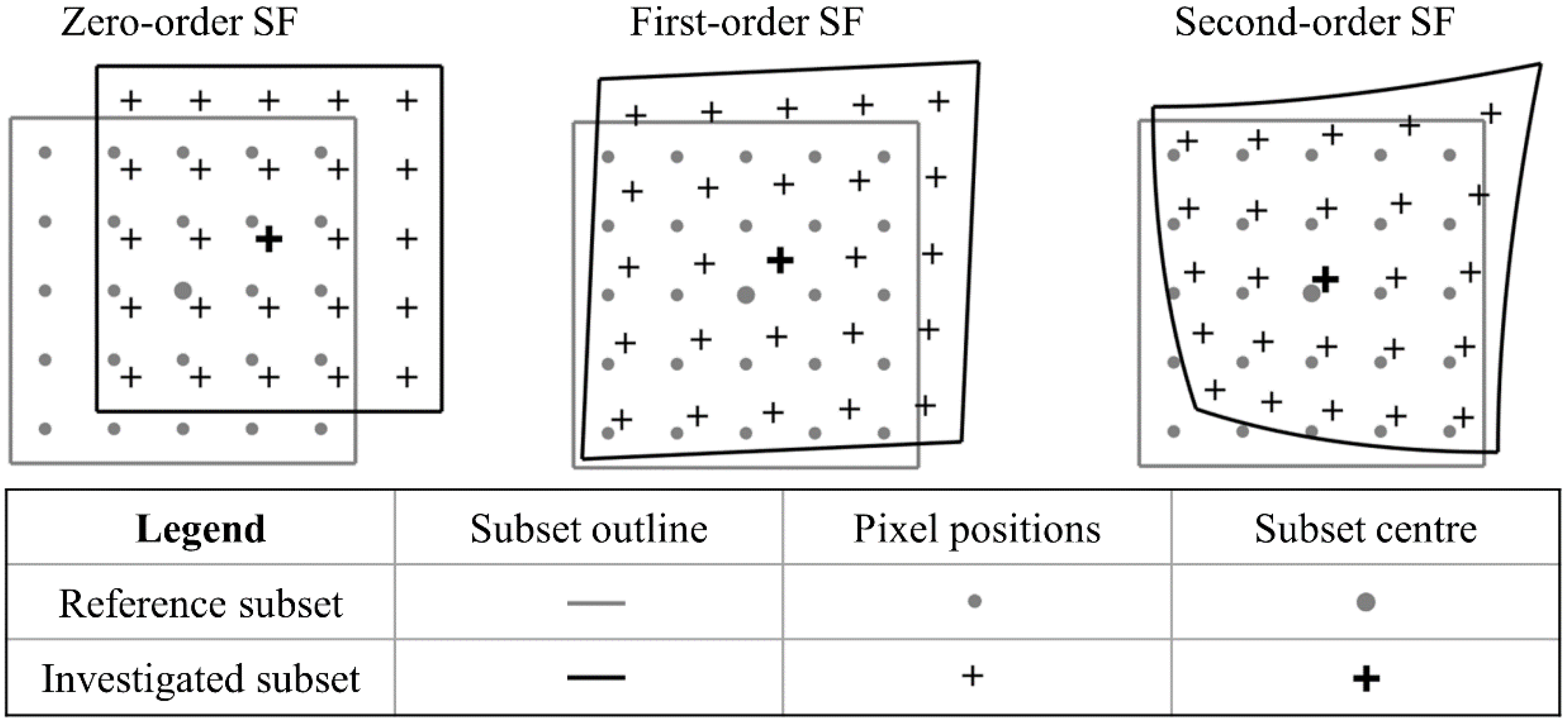
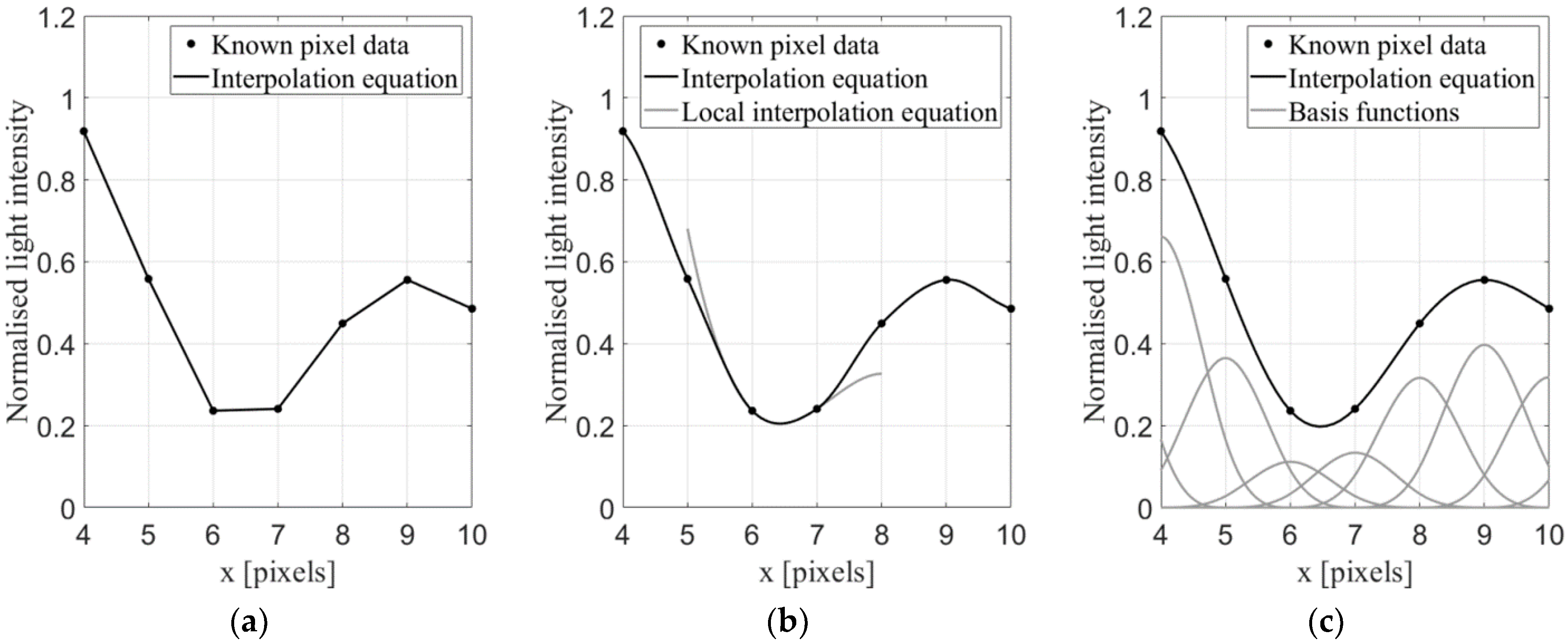
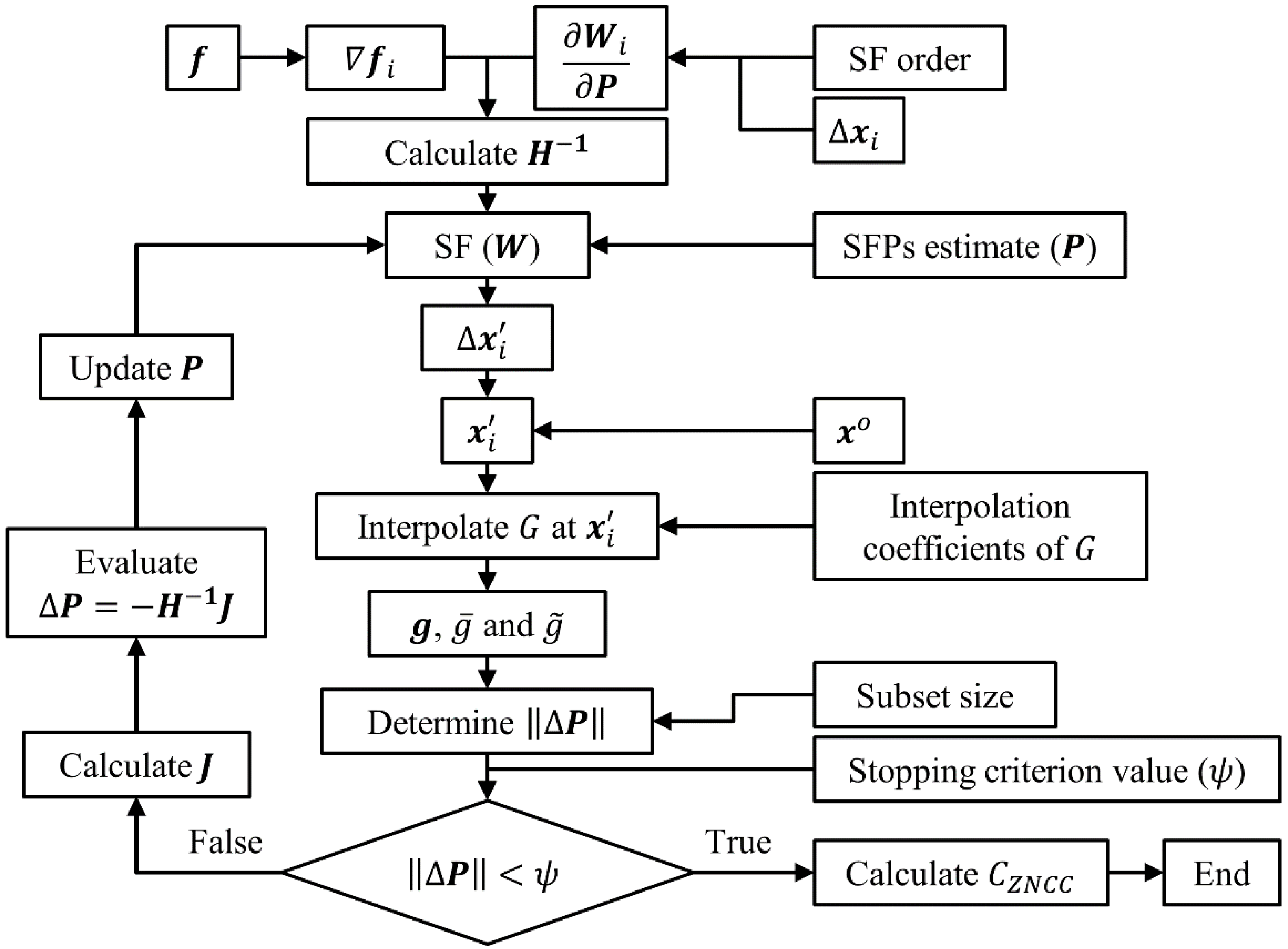
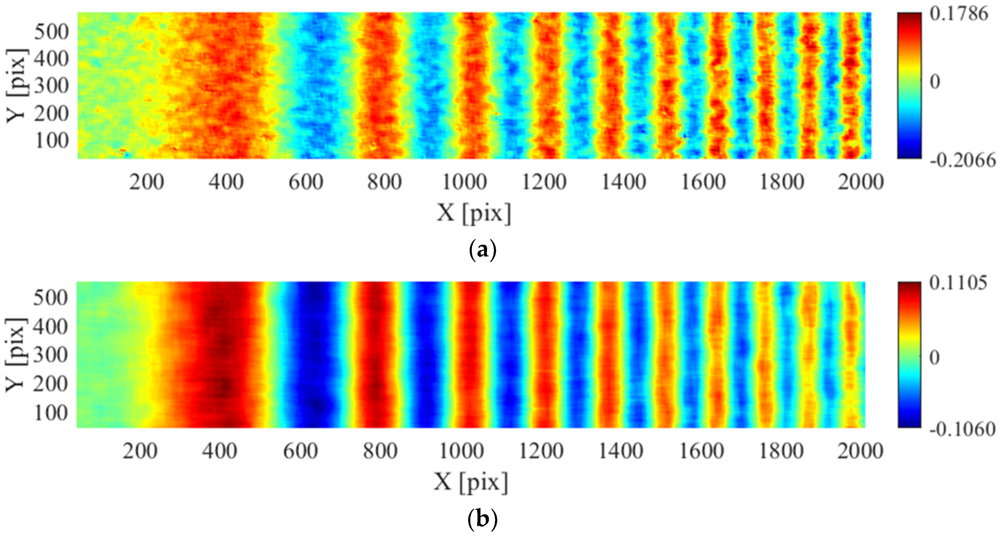
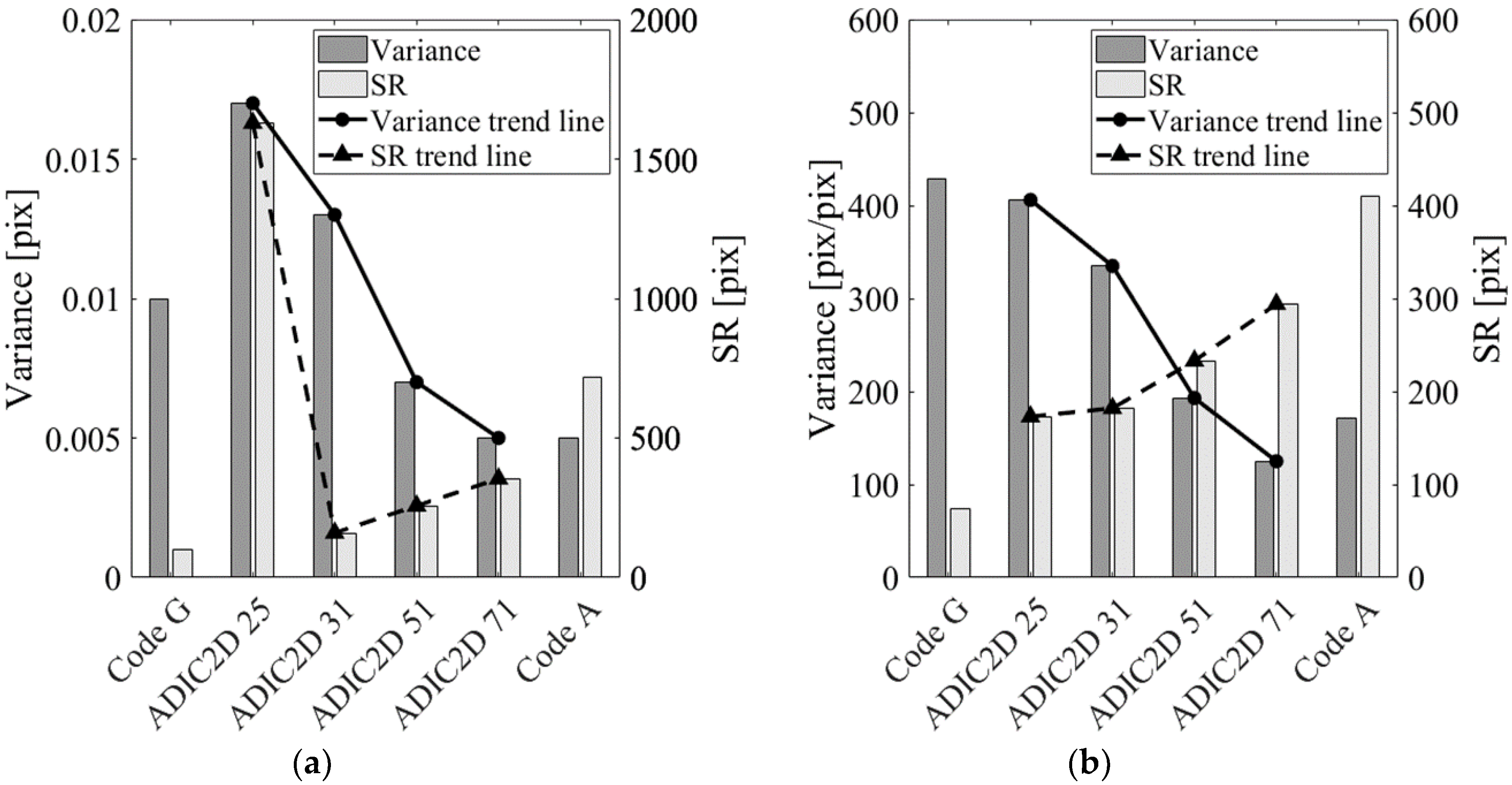
Table 1.
Description of the required input variables for the ADIC2D framework.
| Variable | Variable Description |
|---|---|
| FileNames | Cell array of character vectors containing the image file names of the image set d. All images need to be the same size. |
| Mask | Logical matrix, which is the same size as the images, indicating which pixels should not be analysed during correlation. |
| GaussFilt | Define the standard deviation and window size for the Gaussian filter in pixels as [FiltSigma, FiltSize] respectively where {FiltSigma ∈ ℝ+|FiltSigma > 0} and {FiltSize ∈ ℕ}. |
| StepSize | Step size in pixels {StepSize ∈ ℕ}. |
| SubSize | Subset size in pixels {SubSize = 2k + 1|k ∈ ℕ}. |
| SubShape | Subset shape {SubShape ∈ ‘Square’, ‘Circle’}. |
| SFOrder | Dictates the SF order {SFOrder ∈ ℤ|0 ≤ SFOrder ≤ 2}. |
| RefStrat | Logical statement dictating reference image strategy (Section 3.2). |
| StopCritVal | Defines the stopping criterion value {StopCritVal ∈ ℝ+|StopCritVal > 0}. |
| WorldCTs | Location of CTs in the world CS defined according to MATLAB’s estimateCameraParameters function. |
| ImgCTs | Location of CTs in the sensor CS defined according to MATLAB’s estimateCameraParameters function. |
| rho | Calibration plate thickness in millimetres. |
Table 2.
Accessing the output variables for image d (contained in ProcData(d)) and subset number q.
| Variable | Variable Description |
|---|---|
| ImgName | Image name. |
| ImgSize(b) | Image size (b = 1 for rows and b = 2 for columns). |
| ImgFilt(b) | Standard deviation (b = 1) and window size (b = 2) for the Gaussian filter respectively in pixels. |
| SubSize(q) | Subset size in pixels. |
| SubShape(q) | Subset shape. |
| SFOrder(q) | SF order. |
| Xos(b,q) | Reference subset position in the distorted sensor CS (b = 1 for and b = 2 for ). |
| Xow(b,q) | Reference subset position in the world CS (b = 1 for and b = 2 for ). |
| P(b,q) | SFPs (b = 1 for and b = 7 for ). |
| C(q) | ZNCC coefficient. |
| Uw(b,q) | Displacement in the world CS (b = 1 for and b = 2 for ). |
| Iter(q) | Number of iterations until stopping criterion is satisfied (maximum of 100 iterations). |
| CamParams | Calibration parameters. |
Table 3.
ADIC2D algorithm summary.
| Line Numbers | Task Performed |
|---|---|
| Lines 2–4 | Compute image names, number of images and size of the first image; |
| Lines 5–6 | Create regularly spaced reference subset positions, Xos; |
| Line 7 | Remove subsets containing invalid pixels which are defined by Mask; |
| Line 8 | Pre-assign ProcData structure; |
| Line 9 | Call subroutine ImgCorr to perform image correlation; |
| Line 10 | Call subroutine CSTrans to perform transformation from the distorted sensor CS to the world CS; |
Table 4.
ImgCorr algorithm summary.
| Line Numbers | Task Performed |
|---|---|
| Line 2 | Define SubExtract function to extract square subset data; |
| Line 3 | for image number d = 2 to d = n, do |
| Line 4 | Define G |
| Line 5 | Perform Gaussian filtering on G using MATLAB’s imgaussfilt function; |
| Line 6 | Compute interpolation coefficients using MATLAB’s griddedInterpolant function; |
| Line 7 | if first image of correlation run or Refstrat is incremental, do |
| Line 8 | Define F; |
| Line 9 | Perform Gaussian filtering on F using MATLAB’s imgaussfilt function; |
| Line 10 | Compute gradients for F (compute ); |
| Lines 11–12 | Displace Xos with previous image correlation run displacements (incremental strategy); |
| Line 13 | Call subroutine PCM to compute initial estimates of displacement SFPs; |
| Line 14 | else, do |
| Line 15 | Set P(d) ← P(d − 1); |
| Line 16 | end if |
| Line 17 | Initialise temporary storage variables used to save correlation information during the inner loop; |
| Line 18 | for subset number q = 1 to number of subsets, do |
| Line 19 | Call subroutine SubShapeExtract; |
| Line 20 | Call subroutine SubCorr; |
| Line 21 | end for |
| Line 22 | Save correlation information to PD variable; |
| Line 23–24 | Show results for image d correlation; |
| Line 25 | end for |
Table 5.
SubShapeExtract algorithm summary.
| Line Numbers | Task Performed |
|---|---|
| Line 2 | switch SubShape; |
| Line 3 | case SubShape = ‘Square’, do |
| Line 4–6 | Extract using SubExtract; |
| Line 7 | Compute using SubSize; |
| Line 8 | case SubShape = ‘Circle’, do |
| Line 9–11 | Extract using SubExtract; |
| Line 12 | Compute using SubSize; |
| Line 13 | Determine mask of elements that fall within the circular subset; |
| Line 14–16 | Use mask to extract appropriate data for circular subset; |
| Line 17 | end switch |
Table 6.
SubCorr algorithm summary.
| Line Numbers | Task Performed |
|---|---|
| Line 2 | Call SFExpressions to assign equations dependent on the SF order; |
| Line 3 | ; |
| Line 4 | Compute , Equation (20); |
| Line 5 | Compute normalisation values and ; |
| Line 6 | Initialise flag ← 0, iter ← 0 and ; |
| Line 7 | while flag = 0, do |
| Line 8 | Compute Equation (14), using estimates of P |
| Line 9 | Compute g using interpolation coefficients; |
| Line 10 | Compute normalisation values and ; |
| Line 11 | Compute ‖ΔP‖using Equation (23); |
| Line 12 | if ‖ΔP‖ < StopCritVal or iter > 100, do |
| Line 13 | Set iter ← 1; |
| Line 14 | Compute C, Equation (11) substituted into Equation (13); |
| Line 15 | else, do |
| Line 16 | Compute J, Summation expression of Equation (19); |
| Line 17 | Compute ΔP, Equation (19); |
| Line 18 | Update P, Equation (21); |
| Line 19 | end if |
| Line 20 | Set iter ← iter + 1 |
| Line 21 | end while |
Table 7.
SFExpressions algorithm summary.
| Line Numbers | Task Performed |
|---|---|
| Line 2 | switch SFOrder |
| Line 3–8 | case SFOrder = 0, do assign functions for zero-order SF; |
| Line 9–14 | case SFOrder = 1, do assign functions for first-order SF; |
| Line 15–20 | case SFOrder = 2, do assign functions for second-order SF; |
| Line 21 | end switch |
Table 8.
PCM algorithm summary.
| Line Numbers | Task Performed |
|---|---|
| Line 2 | Compute normalised cross-power spectrum in the frequency domain; |
| Line 3 | Convert back to spatial domain; |
| Line 4 | Find index of the maximum correlation coefficient; |
| Line 5 | Compute index vector which relates indices of the correlation coefficient matrix to the displacements they correspond to; |
| Line 6–7 | Obtain displacements using index of the maximum correlation coefficient; |
Table 9.
CSTrans algorithm summary.
| Line Numbers | Task Performed |
|---|---|
| Line 2 | if calibration targets are given, do |
| Line 3 | Compute calibration parameters using MATLAB’s estimateCameraParameters function; |
| Line 4 | else, do |
| Line 5 | Set unit calibration parameters and pass to MATLAB’s cameraParameters function; |
| Line 6 | Assign CTs in the distorted sensor and world CSs using Xos; |
| Line 7 | end if |
| Line 8 | Extract appropriate extrinsic parameters; |
| Line 9 | Compute , Equation (6); |
| Line 10 | for image number d = 1 to d = n, do |
| Lines 11–12 | Compute , Equation (24); |
| Line 13–14 | Compute and using MATLAB’s undistortPoints and pointsToWorld functions; |
| Line 15 | Compute and , Equation (26); |
| Line 16 | Save calibration parameters; |
| Line 17 | end for |
Table 10.
Details for the samples of the DIC Challenge [39].
Table 10.
Details for the samples of the DIC Challenge [39].
| Name | Method | Noise | Contrast | Images | Displacement field |
|---|---|---|---|---|---|
| Sample 1 | TexGen | 1.5 | Varying | 21 | Shift of 0.05 pixels in both directions per image |
| Sample 2 | TexGen | 8 | 0–50 | 21 | Shift of 0.05 pixels in both directions per image |
| Sample 3 | Fourier | 1.5 | 0–200 | 12 | Shift of 0.1 pixels in both directions per image |
| Sample 14 | Fourier | 5 | 0–200 | 4 | Sinusoid in the x-direction of increasing frequency (amplitude 0.1 pixels) |
Table 11.
Sample 1 error analysis reported at ×10−3 pix.
| Code | Subset Size 21 | Subset Size 41 | Subset Size 81 | ||||||
|---|---|---|---|---|---|---|---|---|---|
| Bias | Variance | RMSE | Bias | Variance | RMSE | Bias | Variance | RMSE | |
| ADIC2D | 2.32 | 2.59 | 3.48 | 1.08 | 0.88 | 1.4 | 0.634 | 0.481 | 0.796 |
| Ncorr | 2.31 | 2.63 | 3.5 | 0.995 | 0.822 | 1.29 | 0.504 | 0.402 | 0.645 |
| DaVis | 1.34 | 1.05 | 1.7 | 0.652 | 0.497 | 0.819 | 0.317 | 0.246 | 0.401 |
Table 12.
Sample 2 error analysis reported at ×10−1 pix.
| Code | Subset Size 21 | Subset Size 41 | Subset Size 81 | ||||||
|---|---|---|---|---|---|---|---|---|---|
| Bias | Variance | RMSE | Bias | Variance | RMSE | Bias | Variance | RMSE | |
| ADIC2D | 3.49 | 4.24 | 5.5 | 1.16 | 0.917 | 1.48 | 0.519 | 0.391 | 0.65 |
| Ncorr | 5.59 | 5.96 | 8.17 | 2.05 | 1.71 | 2.67 | 0.956 | 0.759 | 1.22 |
| DaVis | 1.84 | 1.57 | 2.42 | 0.781 | 0.599 | 0.985 | 0.377 | 0.281 | 0.47 |
Table 13.
Sample 3 error analysis reported at ×10−3 pix.
| Code | Subset Size 21 | Subset Size 41 | Subset Size 81 | ||||||
|---|---|---|---|---|---|---|---|---|---|
| Bias | Variance | RMSE | Bias | Variance | RMSE | Bias | Variance | RMSE | |
| ADIC2D | 9.75 | 8.17 | 12.7 | 3.77 | 2.9 | 4.76 | 1.87 | 1.4 | 2.34 |
| Ncorr | 9.18 | 7.58 | 11.9 | 3.97 | 3.05 | 5.01 | 2.36 | 1.7 | 2.91 |
| DaVis | 5.16 | 4.02 | 6.54 | 2.47 | 1.9 | 3.12 | 1.29 | 1 | 1.64 |
Table 14.
Sample 14 error analysis in the x-direction for last image of the image set [39].
Table 14.
Sample 14 error analysis in the x-direction for last image of the image set [39].
| Code/Subset Size | Displacement | Strain | ||||||
|---|---|---|---|---|---|---|---|---|
| RMSE (pix) | Variance (pix) | Max Bias (pix) | SR (pix) | RMSE (pix/pix) | Variance (pix/pix) | Max Bias (pix/pix) | SR (pix) | |
| Code G | 0.010 | 0.010 | 0.012 | 100 | 453 | 429 | 923 | 74 |
| ADIC2D 25 | 0.018 | 0.017 | 0.015 | 1629 | 598 | 406 | 1488 | 173 |
| ADIC2D 31 | 0.014 | 0.013 | 0.017 | 160 | 600 | 335 | 1674 | 182 |
| ADIC2D 51 | 0.014 | 0.007 | 0.033 | 257 | 839 | 193 | 2720 | 233 |
| ADIC2D 71 | 0.022 | 0.005 | 0.059 | 354 | 1255 | 125 | 4412 | 294 |
| Code A | 0.022 | 0.005 | 0.056 | 716 | 1131 | 172 | 3399 | 410 |
© 2020 by the authors. Licensee MDPI, Basel, Switzerland. This article is an open access article distributed under the terms and conditions of the Creative Commons Attribution (CC BY) license (http://creativecommons.org/licenses/by/4.0/).
Share and Cite
MDPI and ACS Style
Atkinson, D.; Becker, T. A 117 Line 2D Digital Image Correlation Code Written in MATLAB. Remote Sens. 2020, 12, 2906. https://0-doi-org.brum.beds.ac.uk/10.3390/rs12182906
AMA Style
Atkinson D, Becker T. A 117 Line 2D Digital Image Correlation Code Written in MATLAB. Remote Sensing. 2020; 12(18):2906. https://0-doi-org.brum.beds.ac.uk/10.3390/rs12182906
Chicago/Turabian StyleAtkinson, Devan, and Thorsten Becker. 2020. "A 117 Line 2D Digital Image Correlation Code Written in MATLAB" Remote Sensing 12, no. 18: 2906. https://0-doi-org.brum.beds.ac.uk/10.3390/rs12182906
Note that from the first issue of 2016, this journal uses article numbers instead of page numbers. See further details here.