A Feature Space Constraint-Based Method for Change Detection in Heterogeneous Images


1
School of Information and Electronics, Beijing Institute of Technology, Beijing 100081, China
2
Key Laboratory of Network Information System Technology (NIST), Aerospace Information Research Institute, Chinese Academy of Sciences, Beijing 100094, China
*
Author to whom correspondence should be addressed.
Remote Sens. 2020, 12(18), 3057; https://0-doi-org.brum.beds.ac.uk/10.3390/rs12183057
Submission received: 5 August 2020
/
Revised: 14 September 2020
/
Accepted: 15 September 2020
/
Published: 18 September 2020
(This article belongs to the Special Issue Application of Artificial Intelligence in Land Use and Land Cover Mapping)
Abstract
:With the development of remote sensing technologies, change detection in heterogeneous images becomes much more necessary and significant. The main difficulty lies in how to make input heterogeneous images comparable so that the changes can be detected. In this paper, we propose an end-to-end heterogeneous change detection method based on the feature space constraint. First, considering that the input heterogeneous images are in two distinct feature spaces, two encoders with the same structure are used to extract features, respectively. A decoder is used to obtain the change map from the extracted features. Then, the Gram matrices, which include the correlations between features, are calculated to represent different feature spaces, respectively. The squared Euclidean distance between Gram matrices, termed as feature space loss, is used to constrain the extracted features. After that, a combined loss function consisting of the binary cross entropy loss and feature space loss is designed for training the model. Finally, the change detection results between heterogeneous images can be obtained when the model is trained well. The proposed method can constrain the features of two heterogeneous images to the same feature space while keeping their unique features so that the comparability between features can be enhanced and better detection results can be achieved. Experiments on two heterogeneous image datasets consisting of optical and SAR images demonstrate the effectiveness and superiority of the proposed method.
1. Introduction
Change detection (CD) is the process of identifying differences in remote sensing images acquired on the same location, but at different times [1]. It has been widely applied in many fields, such as disaster assessment [2,3], environmental monitoring [4,5], urbanization research [6] and so on.
According to the sources of the utilized images, CD can be divided into homogeneous CD and heterogeneous CD. The images used for homogeneous CD refer to images coming from the sensors with the same or a similar imaging modality, e.g., synthetic aperture radar (SAR) images (SAR-to-SAR) or optical images (optical-to-optical). For heterogeneous CD, the images are acquired by different sensors with different imaging modalities such as SAR and optical images (SAR-to-optical). Different from homogeneous CD, the pixels in heterogeneous images are in different distinct feature spaces [7], and the change map (CM) cannot be obtained by simple linear operations or some homogeneous methods, which is also the main difficulty for heterogeneous CD. Over the past several decades, much attention has been paid to homogeneous CD [8], and many excellent methods have been explored [9,10,11,12,13]. With the increase of different types of satellite sensors, however, CD based on homogeneous images is far away from the practical demands [8] especially when the homogeneous images are not available. For example, when an optical image of a given area is provided by available remote sensing image archive data and only a new SAR image can be acquired (for technical reasons, lack of time, availability, or atmospheric conditions) in an emergency for the same area [14], we can only use the heterogeneous images to detect changes. Thus, it is of great significance to develop novel techniques for CD using heterogeneous images [15]. Currently, the most commonly used images in remote sensing are optical and SAR images. Optical images are acquired by capturing the reflected light of the Sun on different objects, and they are easy to obtain and interpret; however, the optical sensors are easily affected by external conditions, such as weather and sunlight [16]. SAR images measure the reflectivity of ground objects and are not sensitive to environmental conditions, but they are difficult to interpret because of the distance-dependent imaging and the impact of multiple signal reflections [17]. A pair of heterogeneous images consisting of optical and SAR images is complementary and contains much more information than a single SAR image pair or optical image pair. Most heterogeneous CD research, also including the proposed method in this paper, is based on these two types of images.
Recently, the works dedicated to heterogeneous CD can be roughly divided into two categories: classification-based methods and domain transfer-based methods. The former methods first perform pixel- or region-based classification on input heterogeneous images to make them comparable and then compare the processed images to get the final CM. For instance, the widely used post-classification comparison (PCC) methods [18,19] first label two images independently in the pixel level, then compare the labeled images to detect the changes. Besides, Prendes et al. [20] first performed the segmentation of the two images using a region-based approach, then built a similarity measure between images to detect changes based on the unchanged areas. To make full use of the temporal correlations between the input images, Hedhli et al. proposed a cascade strategy, which classifies the current image based on itself and the previous images [21]. Touati et al. [14] tried to build a robust similarity feature map based on the gray levels and local statistics difference and optimized a formulated energy-based model to obtain the final CM. For improvement, Wan et al. [22] used the cooperative multitemporal segmentation to get a set of processed images at different scales and performed a hierarchical compound classification process on them to get the final CM. However, the results of these methods heavily depend on the accuracy of the classification. Furthermore, they are never end-to-end, which means some parameters need to be constantly adjusted to achieve the best results, such as the segmentation scale parameter in [22]. For the domain transfer-based methods, they do not require much preprocessing and mainly transfer two heterogeneous images to the same feature space so that some linear operations or homogeneous approaches can be applied. Specifically, one can transfer two images from their respective feature spaces to the third feature space. For example, Zhao et al. [16] constructed a deep neural network with a coupled structure and transferred the two images to a new feature space so that the CM can be obtained by direct comparison. Touati et al. [23] mapped two heterogeneous images to a common feature space based on the multidimensional scaling (MDS) representation. Liu et al. [24,25] proposed a bipartite differential neural network (BDNN) to extract the holistic features from the unchanged regions in two input images, where two learnable change disguise maps (CDMs) are used to disguise the changed regions in input images. By optimizing the distance between extracted features, the final CM can be obtained with the learned CDMs. In [26], a novel framework for CD based on meta-learning was proposed, which used a convolutional neural network (CNN) to map two images to the same feature space and a graph convolutional network (GCN) to compare samples in the feature space. Besides, one can also transfer the first image from its original feature space to the feature space where the second image is. For example, Zhan et al. [8] proposed a CD method for heterogeneous images based on the logarithmic transformation feature learning framework, which first transfers the SAR image to the feature space where the optical image is so that they have similar statistical distribution properties, then uses a stacked denoising auto-encoder (SDAE) to get the final CM. Niu et al. [27] adopted a conditional generative adversarial network (cGAN) to translate the optical image into the SAR feature space and directly compared the translated image with the approximated SAR image to get the final CM. However, during the transfer process, both of these methods will lose some unique features in their original feature spaces (e.g., some geometric structural features of the shape and boundary in optical images will be lost when they are directly transferred from the optical feature space to the SAR feature space), which may cause some missing detections.
In this paper, an end-to-end heterogeneous CD method based on the feature space constraint is proposed. Compared with the domain transfer-based methods mentioned above, the proposed method can constrain the extracted features to the same feature space while keeping the unique features during the training process. The proposed method first uses Gram matrices, which include the correlations between features, to represent the feature spaces of two heterogeneous images, respectively. Then, the squared Euclidean distance between Gram matrices, termed as feature space loss, is calculated to constrain the features. Similar to the style loss in the style transfer, the feature space loss mainly focuses on constraining the correlations of the features, but not including the content of the features. After that, a combined loss function, consisting of feature space loss and binary cross entropy loss, is designed for training the model. In this way, we can keep as many features of two heterogeneous images as possible during the training process and enhance the comparability between features so that we can get better detection results. Furthermore, considering that the input images are in two distinct feature spaces, we use two encoders with the same structure, but non-shared weights to extract features separately. When training the model, to solve the problem that the numbers of changed and unchanged pixels vary greatly in CD datasets [28], the class balancing is used to weight different parts in the loss function.
The rest of this paper is organized as follows. The background of the proposed method will be introduced in Section 2, and Section 3 will introduce the proposed method in detail. The experimental results on two real heterogeneous CD datasets will be analyzed in Section 4. Finally, the conclusion of this paper will be drawn in Section 5.
2. Background
2.1. Homogeneous Transformation
To make input heterogeneous images comparable, homogeneous transformation is a necessary and significant step for heterogeneous CD, and it can be performed at different levels of the feature spaces.
In the low-level feature spaces, Liu et al. [7,29] used the pixel transformation based on the mapping relationship between unchanged pixel pairs to transfer one image from its original feature space (e.g., gray space) to another feature space (e.g., spectral space) so that the changes between heterogeneous images can be detected. The O-PCC [19], P-PCC [18], and cGAN-based [27] methods mentioned above also usethe homogeneous transformation to make input heterogeneous images comparable in the low-level feature spaces. In the high-level feature spaces, Gong et al. [30] proposed an iterative coupled dictionary learning (CDL) model to establish a pair of coupled dictionaries, which can transfer input heterogeneous images to a common high-dimensional feature space. Jiang et al. [31,32] utilized the deep-level features for homogeneous transformation and built a deep homogeneous feature fusion (DHFT) model to detect the changes in heterogeneous images.
The low-level features contain more spatial information, but they cannot accurately describe the semantic content that is abstract at the high level, especially in the regions with massive ground objects and complex scenes [32]. The high-level features contain more semantic information, but their resolution is usually lower and cannot help us locate where changes occurred precisely. In our method, the homogeneous transformation is realized by the proposed feature space constraint. To make full use of the features at different levels, we perform the proposed feature space constraint for all the extracted features of different levels in input heterogeneous images.
2.2. Style Transfer
Style transfer is usually considered as a generalized problem of texture synthesis, which is to extract and transfer the texture from the source to the target [33]. It is always used to modify the style of an image while still preserving its content.
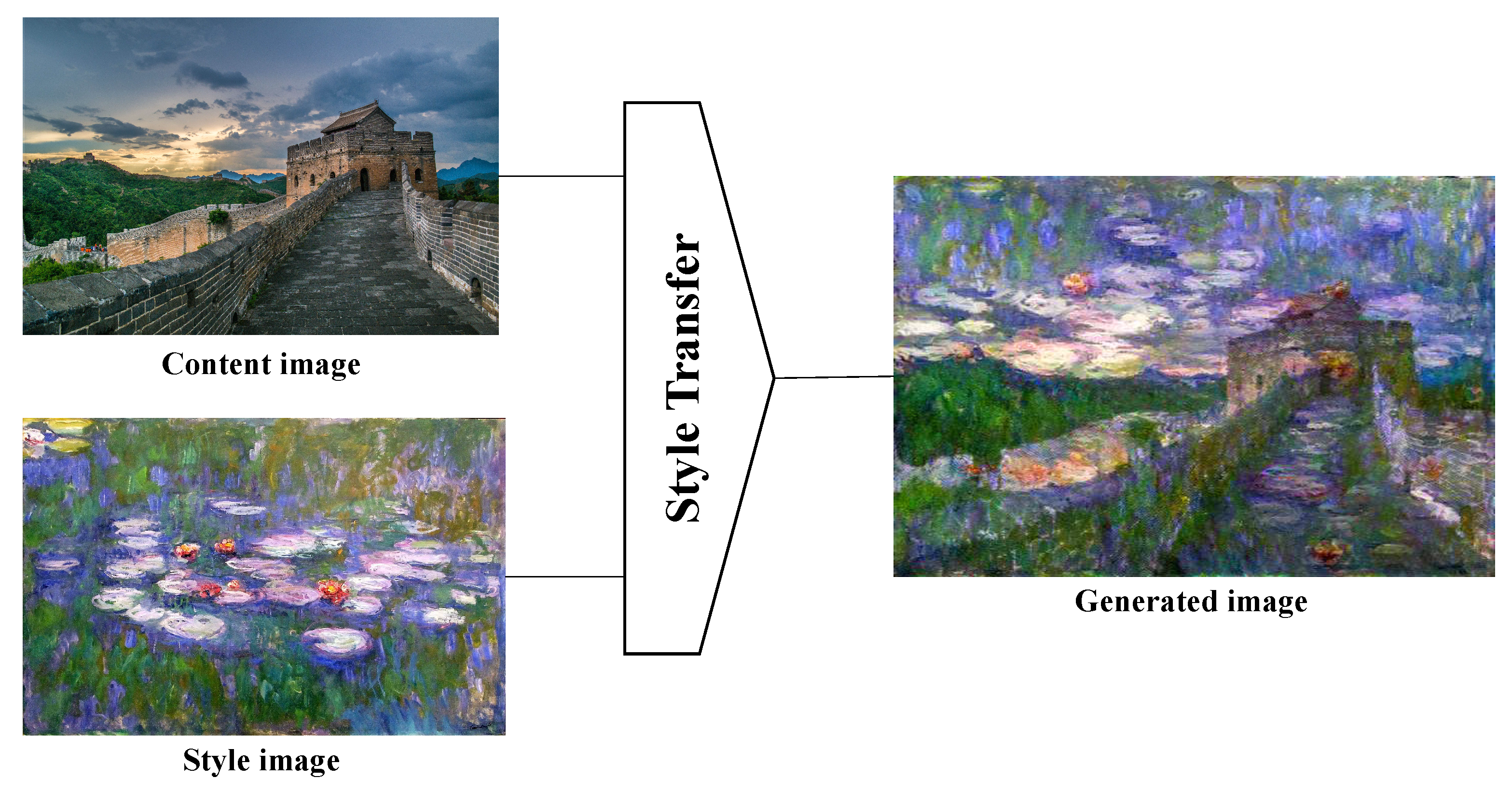
As shown in Figure 1, the input for style transfer is a pair of images. The content image is usually of a nature scene and is responsible for providing content information, while the style image is usually an art image and is responsible for providing style information. With some style transfer algorithms, it will finally generate an image with the provided content information and style information at the same time. Among these algorithms, to produce the transferred images, Gatys et al. [34] used a pre-trained CNN to extract features and optimized the model with the following loss function:
where , , and are the content image, the style image, and the generated image. The content loss is used to minimize the distance of content representation between and . The style loss is used to minimize the distance of style representation between and . The hyperparameters and are the weighting factors for content and style loss, respectively.
In style transfer, to obtain the style representation without including the content information, Gatys et al. [34] used the Gram matrix, which is the correlations between the different filter responses, to represent the feature space of the style image . It should be noted that the content and style representations of images are not completely independent, which means the distance of the style or content representation between source images and target images cannot be minimized separately. Even so, we can still make a tradeoff between style and content representations and produce the desired images by adjusting the weighting factors and .
Inspired by the main idea of style transfer, in this paper, we design a loss function to constrain the correlations between different feature spaces in the form of Gram matrices. Different levels of feature spaces for input paired heterogeneous images are represented by Gram matrices, and a loss function is designed to constrain the correlations between different feature spaces, which is similar to the style loss in style transfer. By minimizing the Gram matrix-based loss function, the features of input heterogeneous images can be constrained to the feature space with the same style (correlations), while the content information is kept, which means the unique features mentioned above.
3. Proposed Method
In this section, how the features are encoded (extracted) and decoded from two heterogeneous images will be first introduced. After that, how the feature space constraint is constructed will be described in three parts: how to represent a feature space while keeping the unique features, how to design the loss function for the feature space constraint, and how to build the final combined loss function for training. Finally, we will summarize the proposed method and give the overall schematic as shown in Figure 2.
For homogeneous CD, Daudt et al. [11] proposed a fully convolutional Siamese network with an autoencoder architecture, which was similar to U-Net [35]. Because the feature spaces of two homogeneous images are very similar, the fully convolutional Siamese network used two encoders with the same structure and shared weights to extract features from the input images X and Y. However, different from homogeneous CD, the images X and Y for heterogeneous CD are in two distinct feature spaces. Therefore, in the encoding part, as shown in Figure 2, we use two encoders with the same structure, but non-shared weights (NSWs) to extract features and from images X and Y, where , is the number of features at the level, and is the product of the height and width of features at the level. It should be noted that, to simplify the calculation, all the extracted features were vectorized, which means (as well as the others) is a matrix composed of the flattened features at the level. For the same reason, in the decoding part, the absolute value of the difference between features and cannot be concatenated directly with the features , which are generated during the decoding process. The l in does not mean that is generated by the Decoder-l, but rather that has the same scale as and at the level. For example, at the fourth level, and are generated by Encoder-4, and is obtained by up-sampling the output of Decoder-5. As shown in Figure 2, the L mentioned above is 5, which means the number of feature scales is 5 in the encoders and 4 in the decoders. This is because we do not have Decoder-6 and therefore cannot get at the fifth level.
The details of the encoders and decoders in the proposed network are shown in Table 1. It should be noted that, in practice, Encoder-5 is not adopted, and the output of Encoder-4 is down-sampled twice, then directly passed to Decoder-5. This is because the datasets used in the experiments are relatively small and simple, and the network must be simplified to avoid overfitting during the training process. As shown in Table 1, the output size of 112 × 112 pixels means that the height and width of the output features in Encoder-1 and Decoder-1 are both 112 pixels. The kernel of 3 × 3 × 1 × 16 means that the size of the kernel is 3 × 3 pixels and the number of input channels and output channels is 1 and 16.
To detect the changes based on the extracted features , , and , we must constrain them to the same feature space, so that they are comparable. However, for two heterogeneous images, they both have their own unique features in their respective feature spaces, which are helpful for the model to detect the changes, and these unique features may be lost if we directly constrain them to the same feature space. For example, the geometric structural features, such as the shape and boundary, in optical images can help locate where the change happened and make the boundary clearer. If we directly transfer the optical images from their original feature space to that of SAR images, these features will be lost during the transfer process. To this end, inspired by the style loss in style transfer, we use the Gram matrices, which calculate the correlations between features, to represent different feature spaces and design a combined loss function based on the Gram matrices. After that, we can constrain the features to the same feature space by minimizing the squared Euclidean distance between Gram matrices in the combined loss function while keeping their own content information. During the training process, the statistical characteristics of features will not be changed, and only the correlations between features are changed, which means as many unique features mentioned above will be kept as possible. In this way, some missing detections will not be caused, and therefore, the CD results can be improved theoretically.
3.1. Feature Space Representation
Before constraining the extracted features , , and to the same feature space, we must characterize their respective feature spaces in the same way. In the proposed method, the Gram matrix, which was introduced in [36] and includes the correlations between features, is applied to represent the feature space. The Gram matrix for features at the level is :
where is the correlation between the feature and the feature:
Similarly, the representations for the feature spaces of and at the level are and :
We can see that the Gram matrix does not include the statistical properties of features such as the mean and variance, but only represents the correlations between features (e.g., the correlation between Features A and B can be regarded as the probability that when Feature A is extracted, Feature B is also extracted). Therefore, how the encoders extract features from two heterogeneous images will not be changed, which means the unique features in their original feature space will not be changed. During the training process, only the correlations between features in , , and are constrained, which is very similar to the style representations in style transfer [34].
3.2. Feature Space Loss
Inspired by the style loss proposed in [34], we use the squared Euclidean distance between Gram matrices to judge whether two feature spaces of heterogeneous images are constrained to the same feature space. Then, the distance between feature spaces of and can be calculated as follows:
Similarly, we can get and . It should be noted that in the layer, we can only get :
To constrain the features to the same feature space while training the model, we add an optimization term, which is related to the feature space distance, into the loss function. The added term is called feature space loss (FSL), and its definition is as follows:
If there is no change between input heterogeneous images, the correlations between features , , and should be the same, which means Gram matrices , , and should also be the same, and the FSL should be zero theoretically. However, if there are some changes between input images, the FSL should not be 0, then should not be used to train the model theoretically. It should be noted that some changes happened, but were not labeled in the ground-truth, and some noise in the images can also affect the extracted features, so that the FSL may not be 0. Nevertheless, as the training goes on, the features corresponding to those useless changes will be ignored, and the noise will be suppressed by the encoders, which can be viewed as a few filters. If the FSL is used to train the model regardless of whether changes happened or not, the model will tend not to detect changes at all, which is not conducive to CD. Because of this, the FSL must be combined with some other loss functions for CD to build the final loss function for training the CD models.
3.3. Combined Loss Function
The most commonly used loss function in CD is BCELoss, and the BCELoss between output O and target (ground-truth) T is:
To solve the imbalance between changed and unchanged pixels in CD datasets, we use the class balancing to weight the BCELoss. The weighted BCELoss is:
where is the number of changed pixels and is the number of unchanged pixels. By weighting the BCELoss, we can expand the positive samples in the training set by times, which is consistent with the number of negative samples, when the number of positive samples is much less than that of negative ones.
Theoretically, when there is no change () in input images, the FSL should be 0, and in contrast (), FSL should be greater than 0. Therefore, we can define the final combined loss:
where is the weighting factor for FSL, and it is also used to ensure that the orders of the magnitude of BCELoss and FSL are consistent.
When training the model, mini-batch gradient descent is often used to update the weights of different modules in the model. However, it is very difficult to find a situation where there is no change at all (T = 0) in the input batch when mini-batch gradient descent is used during the training process. To this end, a threshold is introduced to replace the original T, and the combined loss function is adjusted as follows:
where p is the proportion of changed pixels in the input batch. The threshold is determined in such a way that the frequency proportion of training with in an epoch is basically the same as the proportion of unchanged images in the training set.
3.4. Detailed Change Detection Scheme
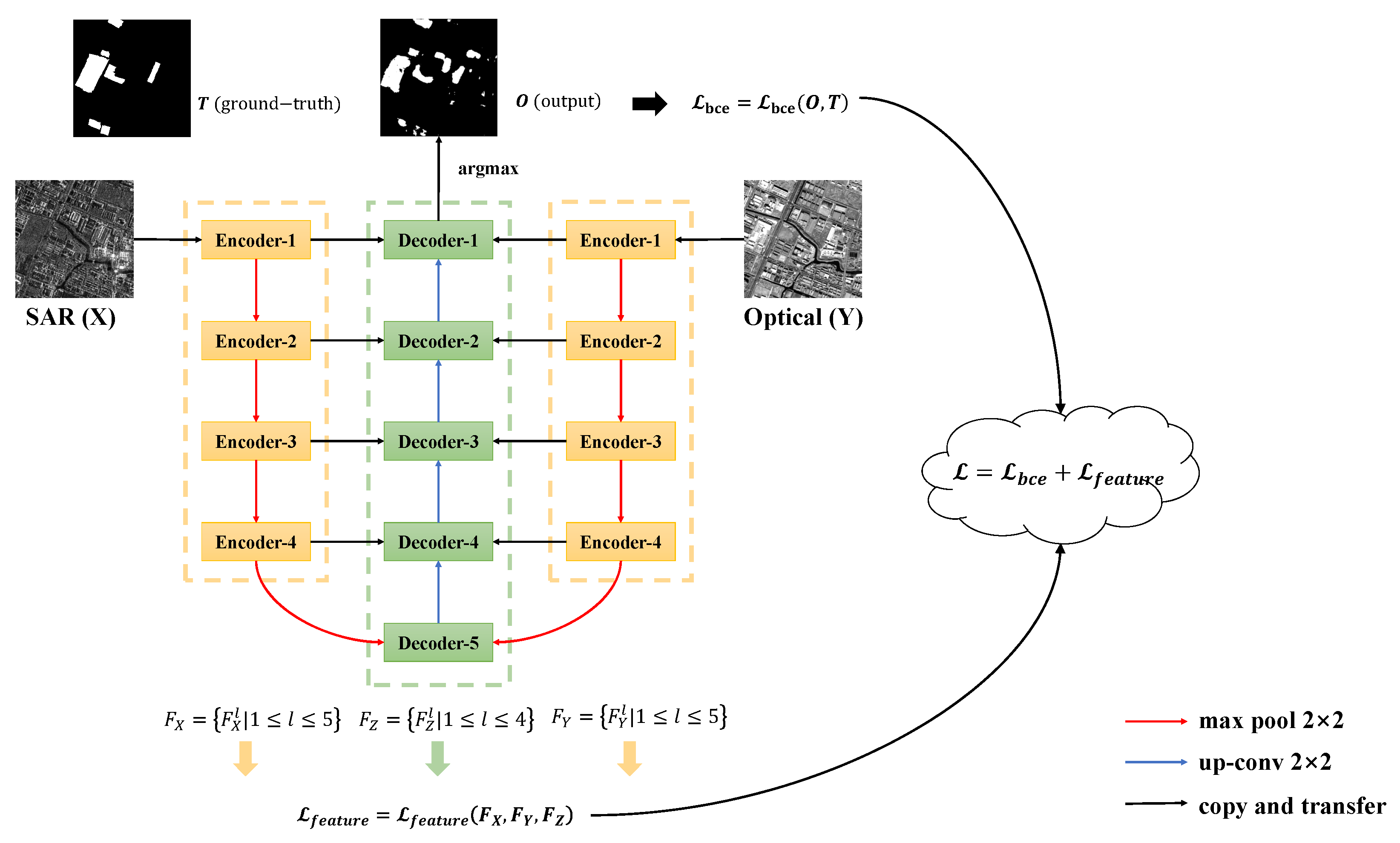
The schematic of the proposed method is shown in Figure 2. First, two encoders with the same structure, but non-shared weights, are used to extract features and from input heterogeneous images X and Y. Next, the absolute value of the difference between the extracted features and is fed to the decoder to output a two-channel probability map, during which the features are generated in the decoding part. For example, Decoder-3 will concatenate the absolute value of the difference between and with the up-sampled output of Decoder-4 as the input and pass the up-sampled output to Decoder-2. Then, a combined loss function consisting of BCELoss and FSL is designed for training the model. BCELoss is the traditional binary cross entropy loss function between the output of the decoder and the one-hot encoded ground-truth. FSL is the feature space loss between the Gram matrices of features , , and . BCELoss will be used throughout the training model, and the use of FSL will be determined by the proportion of changed pixels in the input image pairs. After the model is trained well, the final CM can be obtained by the argmax operation on the channel dimension of the two-channel probability map. Specifically, as shown in Figure 3, the first channel (Channel-0) represents the probabilities that pixels have not changed, while the second channel (Channel-1) represents the probabilities that pixels have changed. In the final CM, 0 represents an unchanged pixel and 1 a changed pixel. Therefore, for pixels in the two channel probability map, we can choose the channel dimension, where the maximum probability is, as the final change detection result. That is the argmax operation on the channel dimension. For example, if the probabilities of some pixels are [0.2, 0.8, 0.4] in Channel-0 and [0.5, 0.2, 0.7] in Channel-1, then after the argmax operation, we can get [1, 0, 1] in the final CM.
4. Experiments
4.1. Dataset Description
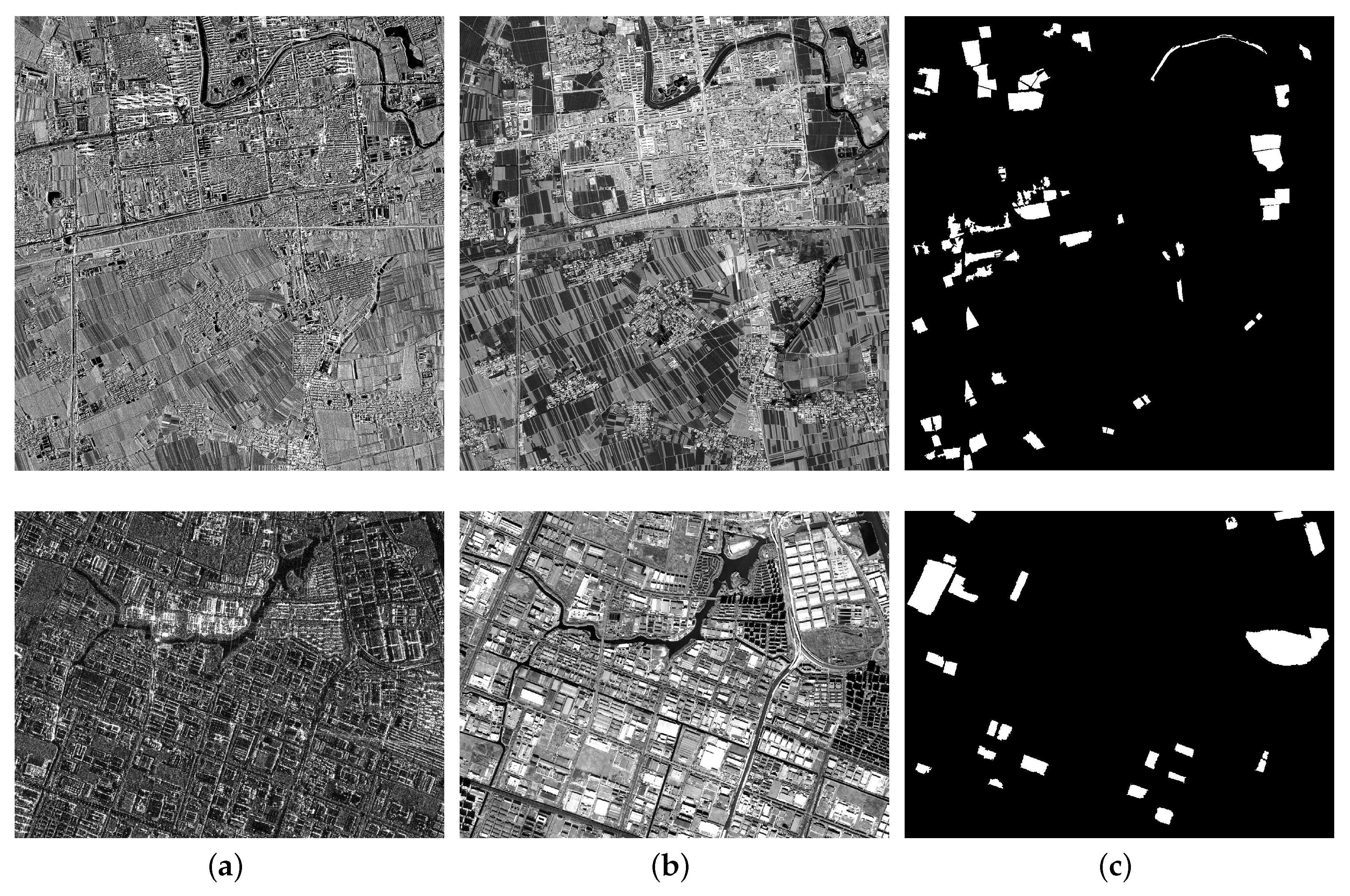
The source images of the datasets that we perform experiments on are from [22]. Considering the distribution of objects and the size of images, as shown in Figure 4, we just select the first and fourth image pair of the four image pairs to make our datasets. It should be noted that the coregistration is a significant step before we detect the changes between images. The first and fourth image pairs are first loosely registered with geographic coordinates and then finely registered by the software ENVI (the environment for visualizing images) with the control points manually selected [22]. To construct the test set, we crop the top-left corner of each image pair to pixels, and the constructed test set (SAR images, optical images, and ground-truth) is shown in Figure 5a–c. The rest of the two images are divided into the training set by a sliding window whose step size is 56 pixels, and the height and width are both 112 pixels, respectively. The details of the two datasets are shown in Table 2.
4.1.1. Dataset-1
The first image pair ( pixels in size) consists of two images that describe the urban areas in Hebei, China. The panchromatic optical image was captured by QuickBird with a 0.6 m resolution, and it was collected on the Google Earth platform. The SAR image was acquired by GaoFen-3 with HH polarization, spotlight (SL) imaging mode, and 1 m resolution. They were registered and resampled to 5 m resolution. The ground-truth is manually defined by integrating expert knowledge with the high resolution historical images in Google Earth (changes are presented in white) [22]. As for the sensors, Google Earth is a platform for Earth science data access and analysis. It integrates the satellite images, aerial photography images, digital elevation model (DEM), and geographic information systems (GISs) onto a 3D globe and then creates giant, multi-terabyte, and high resolution images of the entire Earth [37]. The GaoFen-3 satellite is a C-band multi-polarized SAR satellite in the China High Resolution Earth Observation System [38]. With the mentioned sliding window, we can get 320 training image pairs with a size of pixels and 1 test image pair with a size of pixels. The number of image pairs with no changes entirely is 161, which accounts for 50.3% in the training set. This dataset was created from the first image pair in [22], and to be consistent with the source image pair, we call it Dataset-1.
4.1.2. Dataset-4
The fourth image pair describes the areas near Jiangsu, China. The optical image was a panchromatic image acquired by GaoFen-1 with 2 m resolution. The SAR image was acquired by GaoFen-3 with DH polarization, UFSimaging mode, and 3 m resolution. They were also registered and resampled to 2 m resolution. As for the sensors, GaoFen-1 is a Chinese civil optical remote sensing satellite, which provides panchromatic and multispectral data. The image of GaoFen-1 used in the fourth image pair is the Level-1C product that has been processed by radiation correction [22]. The characteristics of GaoFen-3 were introduced above. Similarly, we can get 376 training samples with a size of pixels and 1 test sample with a size of pixels. It should be noted that, as shown in Table 2, 266 samples (70.7%) in the training set are completely unchanged. This is the common problem mentioned above on CD datasets, that is the imbalance between positive (changed) and negative (unchanged) samples. This dataset was created from the fourth image pair in [22], and to be consistent with the source image pair, we call it Dataset-4.
4.2. Implementation Details
4.2.1. Data Augmentation
As shown in Table 2, the number of images in two training sets is relatively small for training the model, and the size of each image is only pixels, which makes it easier for the model to overfit the datasets. Therefore, data augmentation is necessary for each input image pair in the training sets.
Before each input training pair is input into the network, as shown in Figure 6, it will be first randomly flipped horizontally and vertically, then the flipped image pair will be randomly rotated by a random angle from 0 degrees to 360 degrees. The probability of random horizontal (vertical) flipping is set to 0.5. This is to ensure that the number of samples that have been flipped horizontally (vertically) is basically the same as the number of samples that have not been flipped horizontally (vertically). The probability of random rotation is set to 0.8, which is to ensure that the ratio for the number of unrotated images, rotated images from 0 degrees to 90 degrees, 90 degrees to 180 degrees, 180 degrees to 270 degrees, and 270 degrees to 360 degrees is 1:1:1:1:1. Theoretically, the operation of flipping can expand the dataset to four times its original size, and the operation of rotating can further help augment the training image pairs.
4.2.2. Parameter Setting
The proposed method is implemented using the PyTorch framework, and stochastic gradient descent (SGD) with momentum is applied for optimization. During the training process, the mini-batch size, the base learning rate, the momentum, and the weight decay are set to 32, 0.001, 0.9, and 0.005, respectively. To reduce the training time, the weights of each convolutional layer are initialized with the Kaiming algorithm [39]. To speed up the convergence of the model, the cosine annealing schedule is used to dynamically adjust the learning rate. Besides, according to the analysis above in our approach (see Section 3 for details), for Dataset-1, , , and are set to 12.0, , and 1/40, respectively. For Dataset-4, they are set to 8.0, , and 1/35, respectively.
4.2.3. Evaluation Criteria
To assess the CD results more quantitatively and comprehensively, with respect to the changed pixels, we use overall accuracy (OA), precision (Pr), recall (Re), F1 scores (F1), and the Kappa coefficient (Kappa) [40] as the evaluation criteria. They can be calculated as follows:
where TP is the number of pixels detected by the model and included in the ground-truth images and FP is the number of pixels detected by the model, but not included in the ground-truth images. TN is the number of pixels not detected by the model and not included in the ground-truth images, and FN is the number of pixels not detected by the model, but included in the ground-truth images [41]. represents the percentage of the correct classification, which is equivalent to OA. denotes the proportion of expected agreement between the ground-truth and predictions with given class distributions [42].
Pr and Re refer to the positive predictive value and true positive rate, respectively. F1 is the harmonic mean of Pr and Re. OA shows the classification accuracy of the model, and Kappa is used to evaluate the extent to which the classification results outperform random classification results.
4.3. Results and Evaluation
4.3.1. Experiments’ Design
First, to evaluate the performance of the proposed method, we compare it with several excellent methods on Dataset-1 and Dataset-4: (1) the representation of classic methods: pixel-based PCC (P-PCC) [18] and object-based PCC (O-PCC) [19]; (2) the state-of-the-art (SOTA) methods CMS-HCC (cooperative multitemporal segmentation and hierarchical compound classification) on these two datasets: CMS-HCC (L1), CMS-HCC (L2), and CMS-HCC (L3) [22], where L1, L2, and L3 are three different segmentation scales.
Second, to verify the validity of the NSW in encoders and the FSL in the combined loss function, we perform some experiments on Dataset-1 and Dataset-4 by training the model with or without the NSW or FSL. Furthermore, to investigate why the FSL can improve the CD results, we visualize the curves of the FSL and BCELoss when training the model only with the BCELoss, which aims to find the deeper optimization goal of the FSL.
Finally, to investigate the effect of hyperparameters , , and on the CD results, some experiments are performed with different values of , , and on Dataset-4. Considering the randomness of the experiments and in order to make the results more convincing, each experiment is repeated ten times with different random seeds, and the mean of each criterion is calculated for evaluation.
4.3.2. Comparison with Other Methods
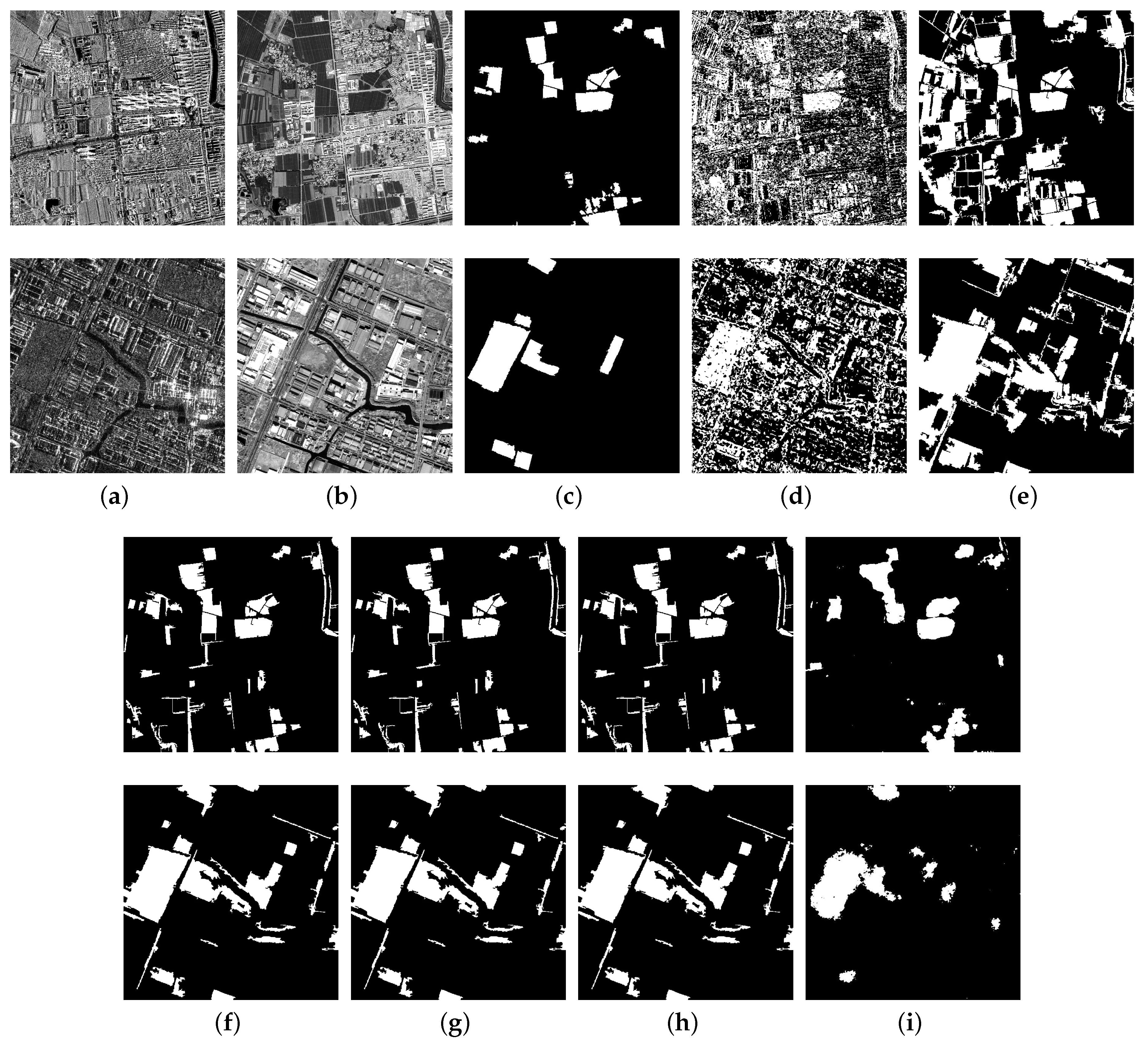
Figure 5 shows the visualized results of all testing methods, and the corresponding quantitative evaluation is presented in Table 3. The best values of each metric on Dataset-1 and Dataset-4 are marked in bold. It should be mentioned that we directly use the results in [22] and crop the top-left with the size of pixels to make a comparison. Although the proposed method is end-to-end, which means it does not need some preprocessing such as segmentation and classification, it can still outperform the other mentioned methods in terms of OA, Kappa, Pr, and F1 on Dataset-1 and Dataset-4.
In terms of OA scores, the proposed method can reach 95.7% on Dataset-1 and 95.2% on Dataset-4, which is higher than 95.1% for CMS-HCC (L2) on Dataset-1 and 93.9% for CMS-HCC (L1) on Dataset-4. Although the OA scores of the CD results for the proposed method and CMS-HCC (L2) on Dataset-1 are very similar, the result of the proposed method is 3.3% higher in Kappa than that of CMS-HCC (L2), which means the proposed method can get better performance when the CD datasets have imbalanced changed and unchanged pixels. Besides, for the F1 scores, the results of the proposed method are nearly 3% and 1% better than other methods on Dataset-1 and on Dataset-4, respectively. Although the O-PCC on Dataset-1 and the CMS-HCC (L3) on Dataset-4 can get the best Re scores (93.3% and 94.8%), they both have many FP pixels, as shown in Figure 5e,h and thus perform very poorly on the Pr scores, which also reduces the F1 scores. According to the results in Table 3, we can see that the CMS-HCC focuses on improving the Pr scores while keeping better Re scores. When compared with the ground-truth in Figure 5c, the CD results of CMS-HCC, as shown in Figure 5f–h, have more TN and FP pixels, which make it able to get better Re scores, but poor Pr scores. Even so, when the Re scores of the proposed method and the CMS-HCC both reach about 80.0% on Dataset-1, the Pr scores of the proposed method can reach 73.5%, while the CMS-HCC can only reach 69.2%. This further demonstrates the superiority of the proposed method. However, compared with the CD results of CMS-HCC, as shown in Figure 5f–h, the boundary of CD results by the proposed method, as shown in Figure 5i, is blurry and discontinuous. This is because the proposed method has some down-sampling and up-sampling modules, which will cause some spatial information to be lost during the feature extraction process. This problem may be solved by some boundary enhancement modules in semantic segmentation [43] and post-processing operations [44].
4.3.3. Experiments on Different Modules of the Proposed Method
Table 4 shows the results of training the model with and without the NSW or the FSL on Dataset-1 and Dataset-4. The best values of each metric on Dataset-1 and Dataset-4 are marked in bold. The NSW means the non-shared weights in encoders, and when it is used, the encoders for input paired heterogeneous images will be trained separately. The FSL is the feature space loss in the combined loss function, and whether it is used determines that the feature space constraint is used or not during the training process.
In the proposed method, if we use the encoders with shared weights, but not NSW to extract features from two heterogeneous images, the CD results will be very poor. When the NSW is adopted in encoders, as shown in Table 4, all the criteria of the model are greatly improved. Specifically, the OA scores increase from 84.7 to 95.4%, and the Kappa scores increase from 40.1 to 72.0%. The Pr scores increase from 34.0 to 72.1%, and the F1 scores increase from 47.5 to 74.5%. However, the Re scores decrease slightly from 78.8 to 77.3%. This is because the model without the NSW cannot extract compared features from two different feature spaces, and many pixels are regarded as changed; therefore, the number of FN pixels decreases, and the Re scores increase.
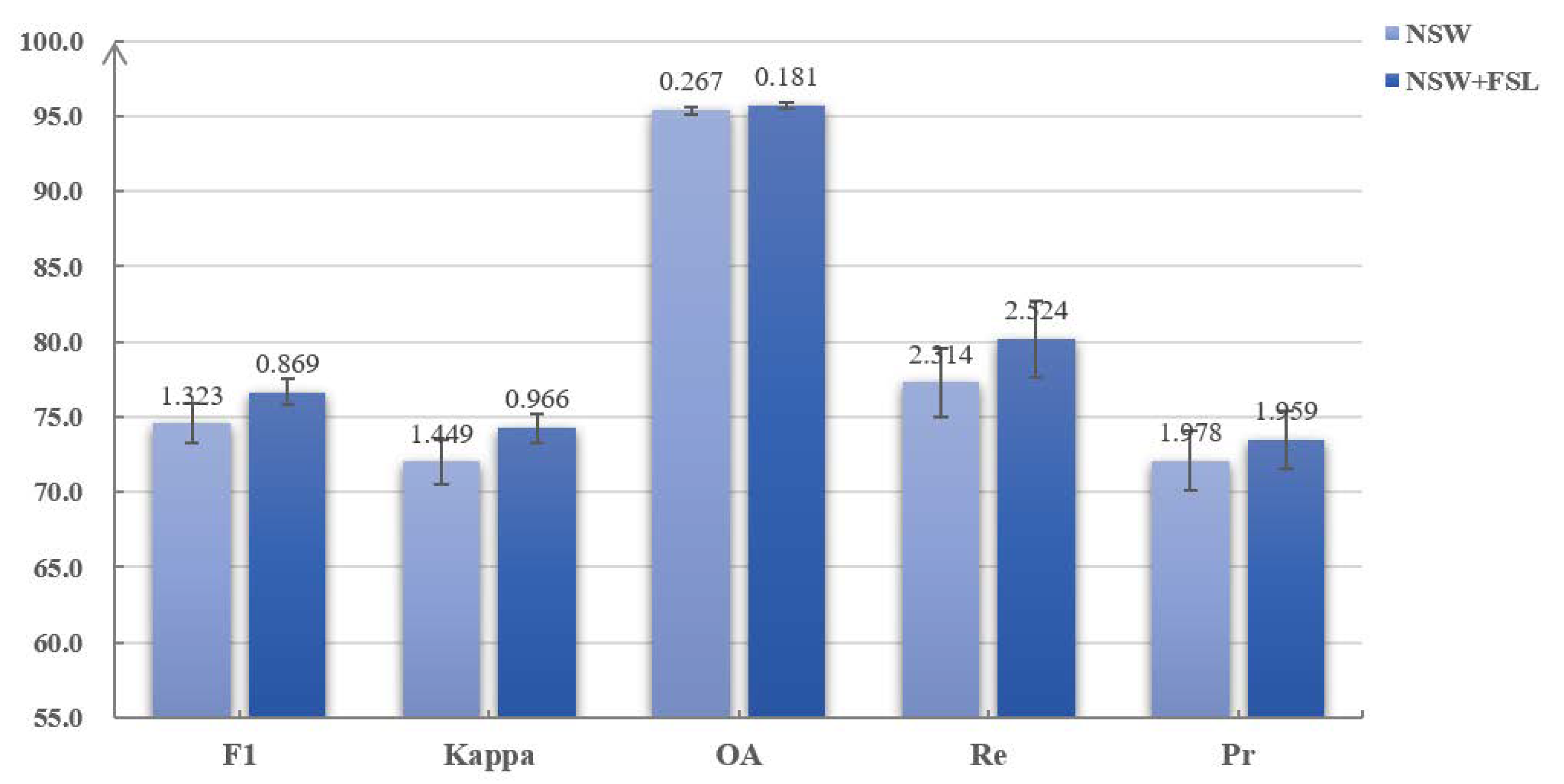
Besides, as shown in Table 4, the CD results can be further improved when the FSL is adopted in the combined loss function. Specifically, on Dataset-1, the Kappa and Re scores are improved by 2%. The F1 and Pr scores are also improved by 1 to 2%. On Dataset-4, the Re scores decrease slightly, while the Pr scores are improved by 4%, which makes the F1 scores increase from 72.1 to 73.6%. In terms of the Kappa and OA scores, the detection results are also improved by 0.8% and 0.5%. Based on the performance of the NSW in encoders and the proposed FSL in the combined loss function, were are convinced that they are both effective for the model and can improve the final CD results. Finally, after visualizing the detection results with error bars, in terms of the standard deviations, on Dataset-1, as shown in Figure 7, we can see that the proposed FSL can also improve the stability of the model, especially when we use the OA, F1, and Kappa scores to assess the model. To sum up, the NSW in encoders makes it possible to detect changes in heterogeneous images with the designed model, and the proposed FSL can further improve the CD results and make the model more stable.
Figure 8 shows the smoothed curves of BCELoss and FSL when training the model on Dataset-4 only with the BCELoss. As shown in Figure 8, when the optimization goal is to minimize the BCELoss, the BCELoss certainty keeps decreasing as the training process goes on. However, it should be noted that the FSL also continues to decrease during the training process even if the feature space constraint is not added to the optimization goal. According to the results in Table 4, we can see that the model still has the ability of mapping two heterogeneous images to the same feature space so that the changes between them can be detected when the model is trained well only with the BCELoss. Thinking about the results in Table 4 and Figure 8, we can conclude that the feature space constraint is implicitly included in the optimization goals even if the model is trained only with the BCELoss. This means that the underlying optimization goal of BCELoss and FSL is very similar. When the FSL is added into the combined loss function, as shown in Equation (14), the implicit constraint becomes explicit. This will further reduce the distance between two feature spaces and exploit the mapping capability of the convolutional neural network, which can therefore improve the final CD results.
4.3.4. Experiments on Different Hyperparameters of the Proposed Method
In the designed loss function, as shown in Equation (14), the hyperparameter is the value of the threshold. It is used to determine whether to use the combined loss function according to the input images. The constant one and hyperparameter are the weighting factors for BCELoss and FSL in the combined loss function.
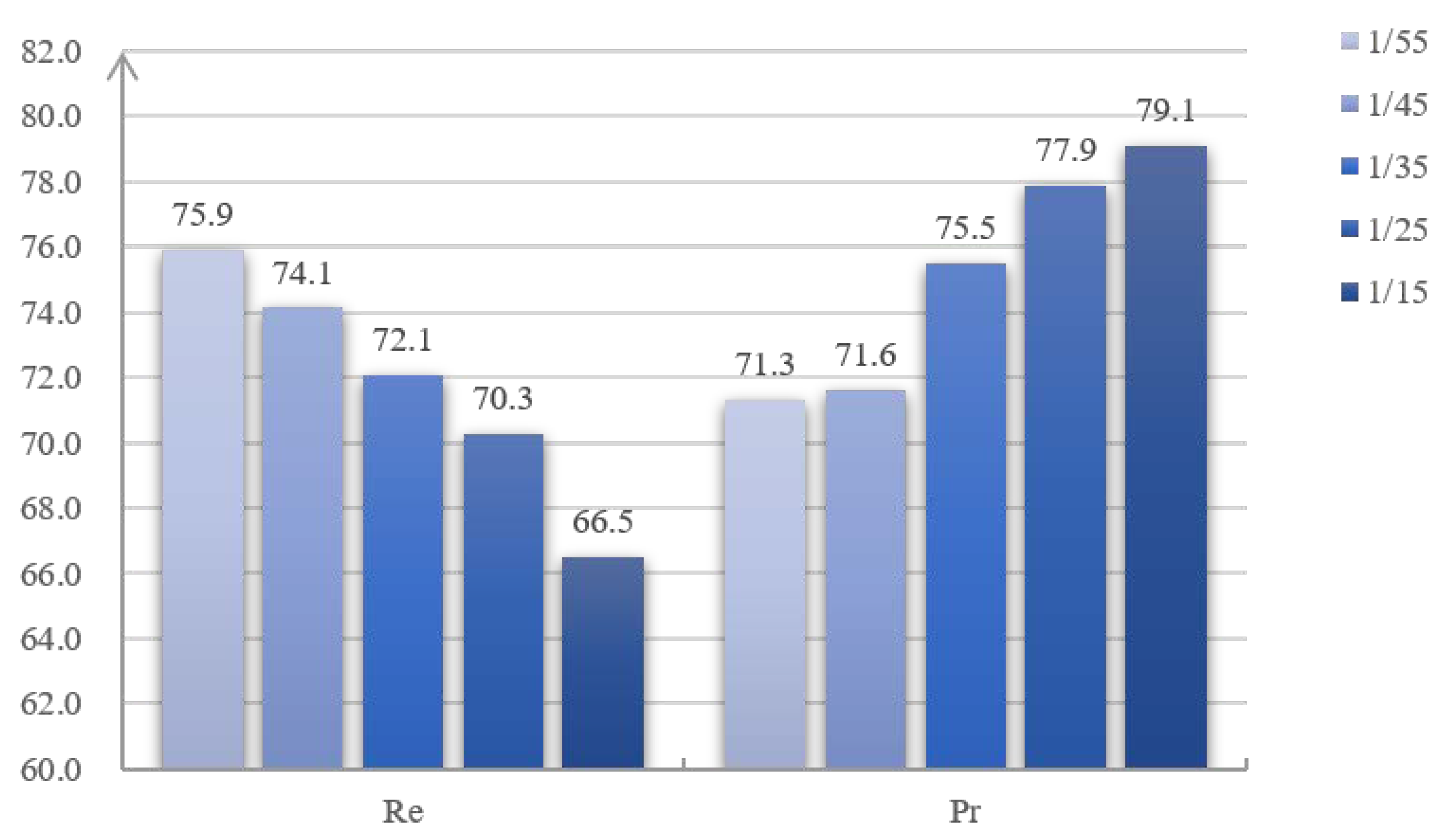
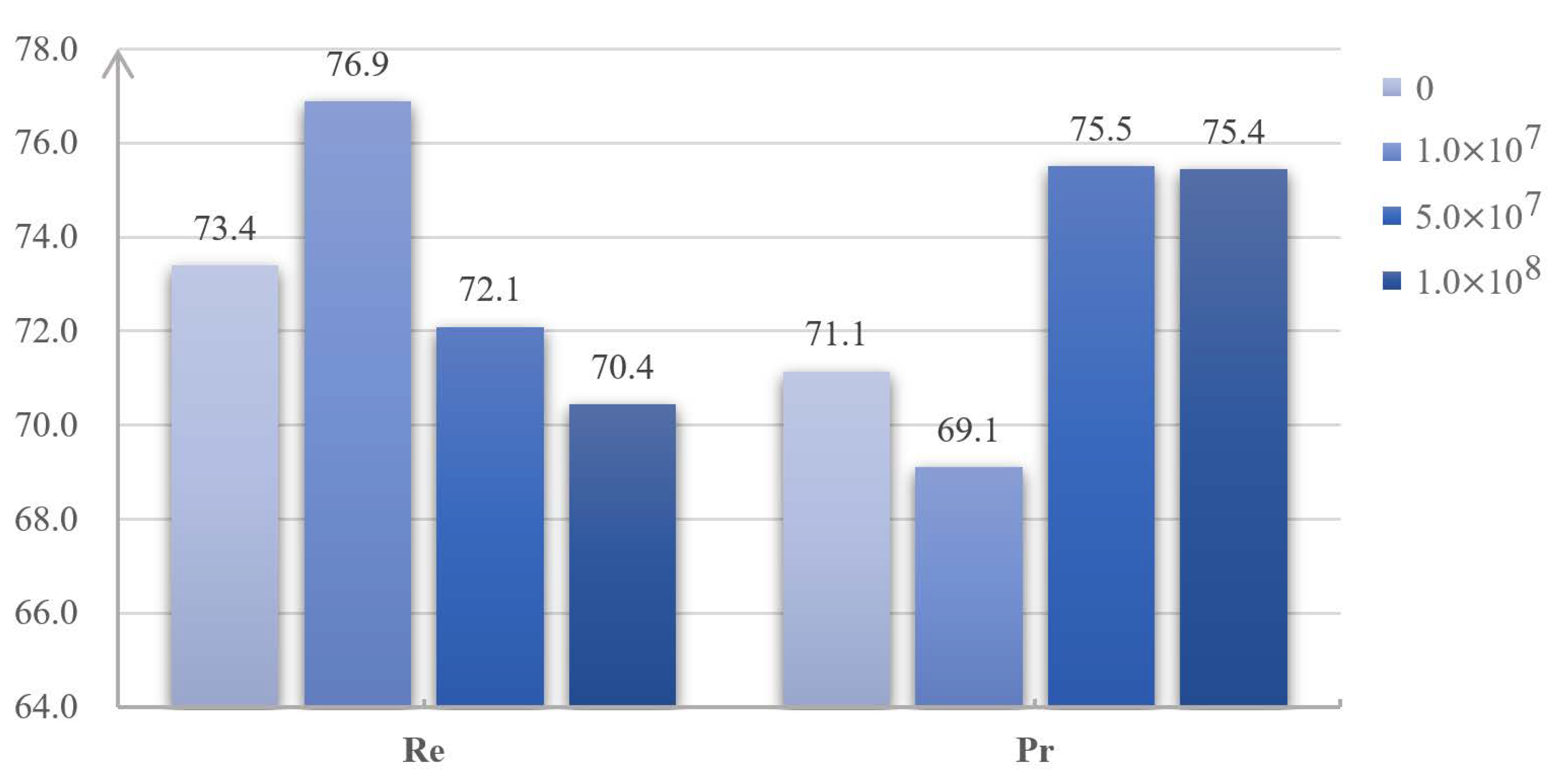
Table 5 and Table 6 show the CD results on Dataset-4 from training with different values of and . According to Equation (14), the greater the value of is, the more likely the combined loss function will be used in the whole training process. Similarly, the greater the value of is, the stricter the feature space constraint between extracted features will become when the combined loss function is used. In other words, the hyperparameters and jointly determine the proportion of the FSL and the BCELoss during the training process. After visualizing the Pr and Re scores of the CD results, as shown in Figure 9 and Figure 10, we can see that the Re scores keep increasing, while the Pr scores keep decreasing when the proportion of FSL becomes higher. For example, when the value of increases from 1/55 to 1/15, the Re scores decrease from 75.9 to 66.5%, while the Pr scoress increase from 71.3 to 79.1%. As introduced in Section 3, the FSL is designed to constrain the features to the same feature space. When the proportion of FSL in the combined loss function becomes higher, it will make the model tend not to detect the changes. If so, the number of FN pixels will decrease while the number of TP pixels will increase. Then, the Re scores, as shown in Equation (21), will decrease, while the corresponding Pr scores will increase. It should be noted that when the value of increases from zero to , almost all the metrics of CD results are improved, but the changes of Re and Pr are irregular. This may be due to the use of the mini-batch gradient descent mentioned above.
To achieve the better performance of the model when training with the designed loss function, we must make a tradeoff between the FSL and the BCELoss, which is similar to the content loss and style loss in style transfer.
In addition to the hyperparameters and , we also perform some experiments on the parameter . As shown in Equation (11), is the weighting factor in the BCELoss and used to solve the imbalance between changed and unchanged pixels on CD datasets. The CD results of training with different values of are shown in Table 7, and the visualized Pr and Re scores of the CD results are shown in Figure 11. As the value of increases, the Re scores keep increasing, while the Pr scores keep decreasing. Specifically, on Dataset-4, when the value of increases from 4.0 to 12.0, the Re scores increase from 67.8 to 77.2%, while the Pr scores decrease from 75.7 to 69.7%. This is because the model will be trained to be more sensitive to the changed pixels when the parameter becomes larger. As shown in Equation (11), when the weight of is increased, the number of TP pixels will increase, while the number of FN pixels will decrease. As shown in Equation (21), the Re scores will be improved, which may lead to a decrease in the Pr scores. To sum up, the model can get better CD results when the balance between the Pr and Re is achieved, which can be made by adjusting the parameter as shown in Equation (12).
5. Discussion
As mentioned above, the main difficulty for heterogeneous CD lies in how to compare the extracted features in input heterogeneous images. First of all, before comparing the features, we must extract them from heterogeneous images. However, different from homogeneous CD, the images for heterogeneous CD are in different feature spaces. Therefore, similar to the symmetric structure in BDNN [25], two encoders with the same structure, but NSWs, are used to extract the features in the proposed method. When the model is trained well, two encoders can extract useful features from input heterogeneous images for CD, separately. As shown in Table 4, we can find that when the NSW is applied in the encoders, the CD results can be highly improved.
Secondly, as described in the Introduction, for the domain transfer-based methods such as cGAN [27] and SCCN [16], some unique features may be lost during the transfer process, which may cause some missing detections. To this end, after the features are extracted, the proposed method uses the Gram matrices, which include the correlations between features, to represent different feature spaces. The features will be constrained to the same feature space by minimizing the squared Euclidean distance between Gram matrices, termed as the FSL. Different from some existing methods of heterogeneous CD [14,29,45], we construct the final loss function by combining the traditional BCELoss and the designed FSL. In this way, we can constrain the correlations between features of different feature spaces to the same feature space, which is similar to the style representations in style transfer. Meanwhile, as many of the unique features of input heterogeneous images will be kept as possible during the training process, which is similar to the content representation in style transfer. As shown in Table 4, when the FSL is used together with the BCELoss for optimizing the model, the final CD results can be further improved. In addition, as shown in Figure 7, we can find that the stability of the model can also be improved when the FSL is used in the optimization goal.
Thirdly, there are three hyperparameters, , , and , in the proposed method. The weighting factor is used in the BCELoss to deal with the imbalance between changed pixels and unchanged pixels in CD datasets. The hyperparameters and in the combined loss function are used to determine the proportions of the BCELoss and the FSL. According to the experimental analysis on these hyperparameters, we can find that the training process, in fact, can be viewed as a game between the FSL and the BCELoss, which is similar to the style loss and content loss in style transfer [34]. When the balance between the FSL and the BCELoss is achieved, the best CD results can be obtained. According to the results of the comparison experiments in Table 3, we can find that our proposed method is superior to other compared methods in terms of OA, Kappa, Pr, and F1 scores. As shown in Figure 5d–h, although the compared methods can get better Re scores, there are so many FP pixels in their CD results that they perform very poorly on the OA, Kappa, and Pr scores, which also reducing the F1 scores.
Finally, as shown in Figure 2, there are some down-sampling and up-sampling modules in the network, which may make some spatial information lost during the feature extraction process. This lost spatial information will make the boundary of objects in the final CM become blurry and discontinuous, as shown in Figure 5i. This problem may be solved by some boundary enhancement modules in semantic segmentation [43] and post-processing operations [44].
6. Conclusions
In this paper, based on the feature space constraint, an end-to-end CD method for heterogeneous images is proposed. For the domain transfer-based methods of heterogeneous CD, there is a problem that some unique features may be lost during the transfer process. In order to solve the problem, inspired by the style transfer, we design a combined loss function based on the FSL and the BCELoss in the proposed method. It can help the model constrain the features of heterogeneous images to the same feature space while keeping as many unique features as possible. In this way, some missing detections will be decreased, and the CD results can be further improved. Additionally, the stability of the model can also be improved when the combined loss function is used. Experiments on two heterogeneous image datasets consisting of optical and SAR images demonstrate the effectiveness and superiority of the proposed method.
In the future, our research will mainly include two aspects. First, as shown in Figure 5, there is the problem of a blurry and discontinuous segmentation boundary, which may be caused by some lost spatial information during the down-sampling. Therefore, in the future work, we will try to use some other architectures such as DeeplabV3 [46] to replace the U-Net architecture or use some boundary enhancement modules in semantic segmentation [43] to make the boundary clearer. Second, according to the analysis in preparing the datasets, we can find that there is a serious imbalance between changed and unchanged samples. The number of changed samples is so small that we must use some methods to augment the change samples, such as the weighting factor in the BCELoss. However, most of these methods cannot actually expand the changed samples. Inspired by some GAN-based methods, we plan to first use GAN to generate some changed samples, then train the model with the generated samples and original datasets. In this way, we can achieve a balance between changed and unchanged samples and maybe improve the CD results.
Author Contributions
N.S. proposed the algorithm and performed the experiments. K.C. gave insightful suggestions for the proposed algorithm. X.S. and G.Z. provided important suggestions for improving the manuscript. All authors read and agreed to the published version of the manuscript.
Funding
This research received no external funding.
Acknowledgments
This work was finished when Nian Shi was an intern at the Key Laboratory of Network Information System Technology (NIST), Aerospace Information Research Institute, Chinese Academy of Sciences.
Conflicts of Interest
The authors declare no conflict of interest.
Abbreviations
The following abbreviations are used in this manuscript:
| BCELoss | binary cross entropy loss |
| BDNN | bipartite differential neural network |
| CD | change detection |
| CDMs | change disguise maps |
| CDL | coupled dictionary learning |
| cGAN | conditional generative adversarial network |
| CM | change map |
| CMS-HCC | cooperative multitemporal segmentation and hierarchical compound classification |
| CNN | convolutional neural network |
| DEM | digital elevation model |
| DHFT | deep homogeneous feature fusion |
| ENVI | Environment for Visualizing Images |
| FSL | feature space loss |
| GCN | graph convolutional network |
| GISs | geographic information systems |
| MDS | multidimensional scaling |
| OA | overall accuracy |
| O-PCC | object-based PCC |
| P-PCC | pixel-based PCC |
| PCC | post-classification comparison |
| Pr | precision |
| Re | recall |
| SAR | synthetic aperture radar |
| SDAE | stacked denoising auto-encoder |
| SGD | stochastic gradient descent |
| NSW | non-shared weight |
References
- Singh, A. Review Article Digital change detection techniques using remotely-sensed data. Int. J. Remote Sens. 1989, 10, 989–1003. [Google Scholar] [CrossRef] [Green Version]
- Giustarini, L.; Hostache, R.; Matgen, P.; Schumann, G.J.P.; Bates, P.D.; Mason, D.C. A Change Detection Approach to Flood Mapping in Urban Areas Using TerraSAR-X. IEEE Trans. Geosci. Remote Sens. 2013, 51, 2417–2430. [Google Scholar] [CrossRef] [Green Version]
- Gueguen, L.; Hamid, R. Toward a Generalizable Image Representation for Large-Scale Change Detection: Application to Generic Damage Analysis. IEEE Trans. Geosci. Remote Sens. 2016, 54, 3378–3387. [Google Scholar] [CrossRef]
- Lunetta, R.S.; Knight, J.F.; Ediriwickrema, J.; Lyon, J.G.; Worthy, L.D. Land-cover change detection using multi-temporal MODIS NDVI data. Remote Sens. Environ. 2006, 105, 142–154. [Google Scholar] [CrossRef]
- Zhu, Z.; Woodcock, C.E. Continuous change detection and classification of land cover using all available Landsat data. Remote Sens. Environ. 2014, 144, 152–171. [Google Scholar] [CrossRef] [Green Version]
- Manonmani, R.; Suganya, G. Remote sensing and GIS application in change detection study in urban zone using multi temporal satellite. Int. J. Geomat. Geosci. 2010, 1, 60–65. [Google Scholar]
- Liu, Z.; Zhang, L.; Li, G.; He, Y. Change Detection in Heterogeneous Remote Sensing Images Based on the Fusion of Pixel Transformation. In Proceedings of the 2017 20th International Conference on Information Fusion (Fusion), Xi’an, China, 10–13 July 2017; pp. 263–268. [Google Scholar] [CrossRef]
- Zhan, T.; Gong, M.; Jiang, X.; Li, S. Log-based transformation feature learning for change detection in heterogeneous images. IEEE Geosci. Remote Sens. Lett. 2018, 15, 1352–1356. [Google Scholar] [CrossRef]
- Pang, S.; Hu, X.; Zhang, M.; Cai, Z.; Liu, F. Co-Segmentation and Superpixel-Based Graph Cuts for Building Change Detection from Bi-Temporal Digital Surface Models and Aerial Images. Remote Sens. 2019, 11, 729. [Google Scholar] [CrossRef] [Green Version]
- Liu, J.; Chen, K.; Xu, G.; Sun, X.; Yan, M.; Diao, W.; Han, H. Convolutional Neural Network-Based Transfer Learning for Optical Aerial Images Change Detection. IEEE Geosci. Remote Sens. Lett. 2020, 17, 127–131. [Google Scholar] [CrossRef]
- Daudt, R.C.; Saux, B.L.; Boulch, A. Fully Convolutional Siamese Networks for Change Detection. In Proceedings of the 2018 25th IEEE International Conference on Image Processing (ICIP), Athens, Greece, 7–10 October 2018; pp. 4063–4067. [Google Scholar] [CrossRef] [Green Version]
- Zhang, M.; Xu, G.; Chen, K.; Yan, M.; Sun, X. Triplet-based semantic relation learning for aerial remote sensing image change detection. IEEE Geosci. Remote Sens. Lett. 2018, 16, 266–270. [Google Scholar] [CrossRef]
- Liu, J.; Chen, K.; Xu, G.; Li, H.; Yan, M.; Diao, W.; Sun, X. Semi-Supervised Change Detection Based on Graphs with Generative Adversarial Networks. In Proceedings of the 2019 IEEE International Geoscience and Remote Sensing Symposium, Yokohama, Japan, 28 July–2 August 2019; pp. 74–77. [Google Scholar] [CrossRef]
- Touati, R.; Mignotte, M. An energy-based model encoding nonlocal pairwise pixel interactions for multisensor change detection. IEEE Trans. Geosci. Remote Sens. 2017, 56, 1046–1058. [Google Scholar] [CrossRef]
- Brunner, D.; Lemoine, G.; Bruzzone, L. Earthquake damage assessment of buildings using VHR optical and SAR imagery. IEEE Trans. Geosci. Remote Sens. 2010, 48, 2403–2420. [Google Scholar] [CrossRef] [Green Version]
- Zhao, W.; Wang, Z.; Gong, M.; Liu, J. Discriminative Feature Learning for Unsupervised Change Detection in Heterogeneous Images Based on a Coupled Neural Network. IEEE Trans. Geosci. Remote Sens. 2017, 55, 7066–7080. [Google Scholar] [CrossRef]
- Auer, S.; Hornig, I.; Schmitt, M.; Reinartz, P. Simulation-Based Interpretation and Alignment of High-Resolution Optical and SAR Images. IEEE J. Sel. Top. Appl. Earth Observ. Remote Sens. 2017, 10, 4779–4793. [Google Scholar] [CrossRef] [Green Version]
- Mubea, K.; Menz, G. Monitoring Land-Use Change in Nakuru (Kenya) Using Multi-Sensor Satellite Data. Adv. Remote Sens. 2012, 1, 74–84. [Google Scholar] [CrossRef] [Green Version]
- Zhou, W.; Troy, A.; Grove, M. Object-based Land Cover Classification and Change Analysis in the Baltimore Metropolitan Area Using Multitemporal High Resolution Remote Sensing Data. Sensors 2008, 8, 1613–1636. [Google Scholar] [CrossRef] [Green Version]
- Prendes, J.; Chabert, M.; Pascal, F.; Giros, A.; Tourneret, J.Y. Change detection for optical and radar images using a Bayesian nonparametric model coupled with a Markov random field. In Proceedings of the 2015 IEEE International Conference on Acoustics, Speech and Signal Processing (ICASSP), South Brisbane, Australia, 19–24 April 2015; pp. 1513–1517. [Google Scholar]
- Hedhli, I.; Moser, G.; Zerubia, J.; Serpico, S.B. A New Cascade Model for the Hierarchical Joint Classification of Multitemporal and Multiresolution Remote Sensing Data. IEEE Trans. Geosci. Remote Sens. 2016, 54, 6333–6348. [Google Scholar] [CrossRef] [Green Version]
- Wan, L.; Xiang, Y.; You, H. An Object-Based Hierarchical Compound Classification Method for Change Detection in Heterogeneous Optical and SAR Images. IEEE Trans. Geosci. Remote Sens. 2019, 57, 9941–9959. [Google Scholar] [CrossRef]
- Touati, R.; Mignotte, M.; Dahmane, M. Change Detection in Heterogeneous Remote Sensing Images Based on an Imaging Modality-Invariant MDS Representation. In Proceedings of the 2018 25th IEEE International Conference on Image Processing (ICIP), Athens, Greece, 7–10 October 2018; pp. 3998–4002. [Google Scholar] [CrossRef]
- Liu, J.; Gong, M.; Qin, K.; Zhang, P. A deep convolutional coupling network for change detection based on heterogeneous optical and radar images. IEEE Trans. Neural Netw. Learn. Syst. 2016, 29, 545–559. [Google Scholar] [CrossRef]
- Liu, J.; Gong, M.; Qin, A.K.; Tan, K.C. Bipartite Differential Neural Network for Unsupervised Image Change Detection. IEEE Trans. Neural Netw. Learn. Syst. 2019, 31, 876–890. [Google Scholar] [CrossRef]
- Liu, H.; Wang, Z.; Shang, F.; Zhang, M.; Gong, M.; Ge, F.; Jiao, L. A Novel Deep Framework for Change Detection of Multi-source Heterogeneous Images. In Proceedings of the 2019 International Conference on Data Mining Workshops (ICDMW), Beijing, Chin, 8–11 November 2019; pp. 165–171. [Google Scholar]
- Niu, X.; Gong, M.; Zhan, T.; Yang, Y. A Conditional Adversarial Network for Change Detection in Heterogeneous Images. IEEE Geosci. Remote Sens. Lett. 2019, 16, 45–49. [Google Scholar] [CrossRef]
- Zhan, Y.; Fu, K.; Yan, M.; Sun, X.; Wang, H.; Qiu, X. Change Detection Based on Deep Siamese Convolutional Network for Optical Aerial Images. IEEE Geosci. Remote Sens. Lett. 2017, 14, 1845–1849. [Google Scholar] [CrossRef]
- Liu, Z.; Li, G.; Mercier, G.; He, Y.; Pan, Q. Change Detection in Heterogenous Remote Sensing Images via Homogeneous Pixel Transformation. IEEE Trans. Image Process. 2018, 27, 1822–1834. [Google Scholar] [CrossRef] [PubMed]
- Gong, M.; Zhang, P.; Su, L.; Liu, J. Coupled Dictionary Learning for Change Detection From Multisource Data. IEEE Trans. Geosci. Remote Sens. 2016, 54, 7077–7091. [Google Scholar] [CrossRef]
- Jiang, X.; Li, G.; Liu, Y.; Zhang, X.P.; He, Y. Homogeneous Transformation Based on Deep-Level Features in Heterogeneous Remote Sensing Images. In Proceedings of the 2019 IEEE International Geoscience and Remote Sensing Symposium, Yokohama, Japan, 28 July–2 August 2019; pp. 206–209. [Google Scholar] [CrossRef]
- Jiang, X.; Li, G.; Liu, Y.; Zhang, X.P.; He, Y. Change Detection in Heterogeneous Optical and SAR Remote Sensing Images Via Deep Homogeneous Feature Fusion. IEEE J. Sel. Top. Appl. Earth Observ. Remote Sens. 2020, 13, 1551–1566. [Google Scholar] [CrossRef] [Green Version]
- Jing, Y.; Yang, Y.; Feng, Z.; Ye, J.; Yu, Y.; Song, M. Neural Style Transfer: A Review. IEEE Trans. Vis. Comput. Graph. 2019. [Google Scholar] [CrossRef] [Green Version]
- Gatys, L.A.; Ecker, A.S.; Bethge, M. Image Style Transfer Using Convolutional Neural Networks. In Proceedings of the 2016 IEEE Conference on Computer Vision and Pattern Recognition (CVPR), Las Vegas, NV, USA, 27–30 June 2016; pp. 2414–2423. [Google Scholar] [CrossRef]
- Ronneberger, O.; Fischer, P.; Brox, T. U-Net: Convolutional Networks for Biomedical Image Segmentation; Lecture Notes in Computer Science; Springer International Publishing: Berlin/Heidelberg, Germany, 2015; pp. 234–241. [Google Scholar] [CrossRef] [Green Version]
- Gatys, L.; Ecker, A.S.; Bethge, M. Texture Synthesis Using Convolutional Neural Networks. In Advances in Neural Information Processing Systems 28; Curran Associates, Inc.: Red Hook, NY, USA, 2015; pp. 262–270. [Google Scholar]
- Yu, L.; Gong, P. Google Earth as a virtual globe tool for Earth science applications at the global scale: Progress and perspectives. Int. J. Remote Sens. 2012, 33, 3966–3986. [Google Scholar] [CrossRef]
- Qingjun, Z. System design and key technologies of the GF-3 satellite. Acta Geod. Et Cartogr. Sin. 2017, 46, 269. [Google Scholar]
- He, K.; Zhang, X.; Ren, S.; Sun, J. Delving Deep into Rectifiers: Surpassing Human-Level Performance on ImageNet Classification. In Proceedings of the 2015 IEEE International Conference on Computer Vision (ICCV), Santiago, Chile, 7–13 December 2015; pp. 1026–1034. [Google Scholar] [CrossRef] [Green Version]
- Brennan, R.L.; Prediger, D.J. Coefficient Kappa: Some Uses, Misuses, and Alternatives. Educ. Psychol. Meas. 1981, 41, 687–699. [Google Scholar] [CrossRef]
- Li, S.; Tang, H.; Huang, X.; Mao, T.; Niu, X. Automated Detection of Buildings from Heterogeneous VHR Satellite Images for Rapid Response to Natural Disasters. Remote Sens. 2017, 9, 1177. [Google Scholar] [CrossRef] [Green Version]
- El Amin, A.M.; Liu, Q.; Wang, Y. Zoom out CNNs features for optical remote sensing change detection. In Proceedings of the 2017 2nd International Conference on Image, Vision and Computing (ICIVC), Chengdu, China, 2–4 June 2017; pp. 812–817. [Google Scholar]
- Yu, C.; Wang, J.; Peng, C.; Gao, C.; Yu, G.; Sang, N. Learning a Discriminative Feature Network for Semantic Segmentation. In Proceedings of the 2018 IEEE/CVF Conference on Computer Vision and Pattern Recognition, Salt Lake City, UT, USA, 18–22 June 2018. [Google Scholar] [CrossRef] [Green Version]
- Wang, H.; Moss, R.H.; Chen, X.; Stanley, R.J.; Stoecker, W.V.; Celebi, M.E.; Malters, J.M.; Grichnik, J.M.; Marghoob, A.A.; Rabinovitz, H.S.; et al. Modified watershed technique and post-processing for segmentation of skin lesions in dermoscopy images. Comput. Med. Imaging Graph. 2011, 35, 116–120. [Google Scholar] [CrossRef] [PubMed] [Green Version]
- Yang, M.J.; Jiao, L.C.; Liu, F.; Hou, B.; Yang, S.Y. Transferred Deep Learning-Based Change Detection in Remote Sensing Images. IEEE Trans. Geosci. Remote Sens. 2019, 57, 6960–6973. [Google Scholar] [CrossRef]
- Chen, L.C.; Papandreou, G.; Kokkinos, I.; Murphy, K.; Yuille, A.L. Deeplab: Semantic image segmentation with deep convolutional nets, atrous convolution, and fully connected crfs. IEEE Trans. Pattern Anal. Mach. Intell. 2017, 40, 834–848. [Google Scholar] [CrossRef] [PubMed]
Figure 1.
An example of style transfer. Style transfer can be viewed as a process of generating an image , which has the content information of a content image and the style information of a style image at the same time.
Figure 1.
An example of style transfer. Style transfer can be viewed as a process of generating an image , which has the content information of a content image and the style information of a style image at the same time.

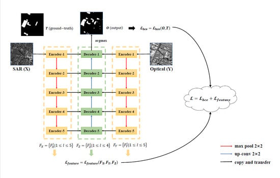
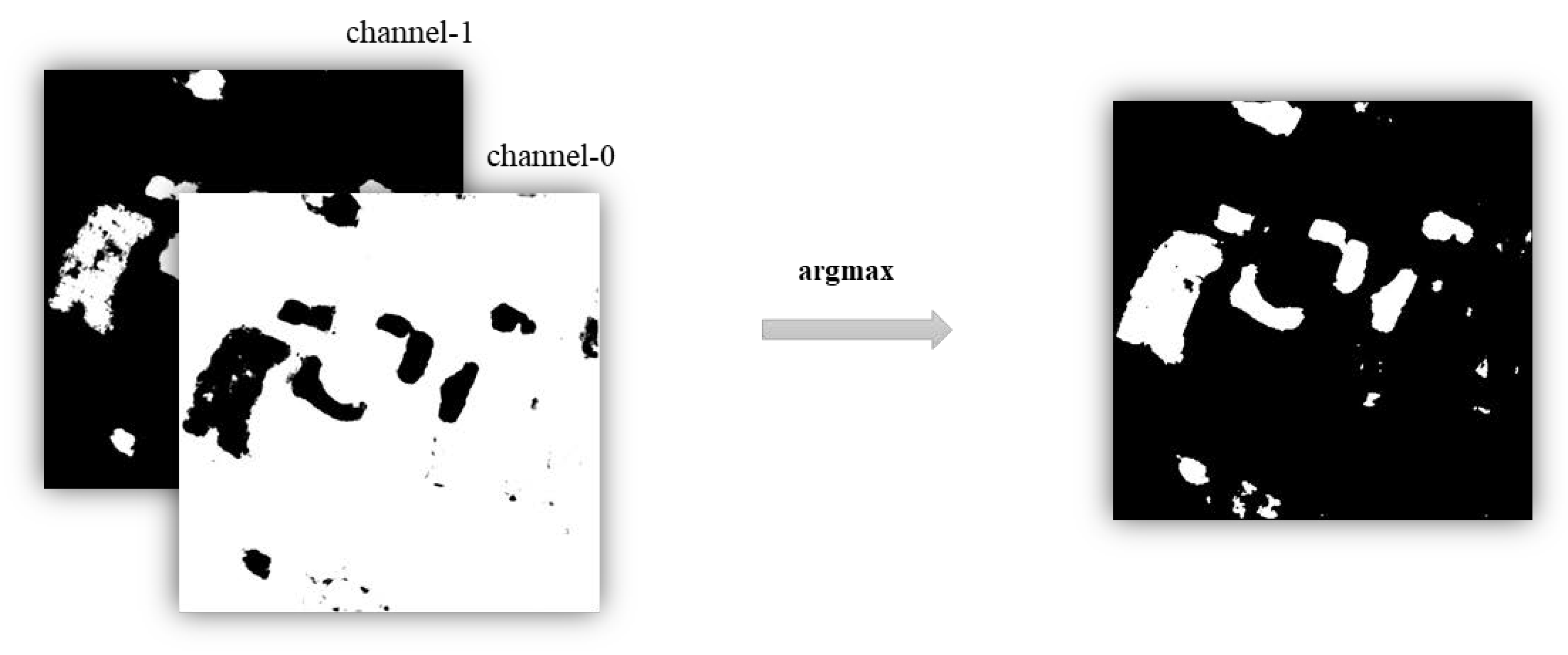
Figure 2.
Schematic of the proposed feature space constraint-based change detection method for heterogeneous images. The red lines represent down-sampling, while the blue lines represent up-sampling. The black lines only indicate the direction of information transfer. is the feature space loss among features , , and , and it is used to constrain the features to the same feature space. is the binary cross entropy between the output and ground-truth, and it is used to train the model to detect the changed pixels in input image pairs. means and are jointly used for training the model.

Figure 3.
The argmax operation on the channel dimension of the two channel probability map.

Figure 4.
Source images of Dataset-1 and Dataset-4. First row: Dataset-1, second row: Dataset-4. For Dataset-1 in the first row, the panchromatic optical image was captured by QuickBird on 28 May 2006, and the SAR image was acquired by GaoFen-3 with HH polarization, spotlight imaging mode, on 19 October 2016 in Heibei, China. For Dataset-4 in the second row, the images were captured in Jiangsu, China, and they were acquired by GaoFen-2 on 1 January 2015 and GaoFen-3 with DH polarization, UFSimaging mode, on 23 July 2018, separately. (a) SAR images. (b) Optical images. (c) Ground-truth.

Figure 5.
Results of the different methods. The first row is Dataset-1, and the second row is Dataset-4. (a) SAR images. (b) Optical images. (c) Ground-truth. (d–i) are the change maps produced by: (d) P-PCC; (e) O-PCC; (f) CMS-HCC (L1); (g) CMS-HCC (L2); (h) CMS-HCC (L3); (i) proposed method.
Figure 5.
Results of the different methods. The first row is Dataset-1, and the second row is Dataset-4. (a) SAR images. (b) Optical images. (c) Ground-truth. (d–i) are the change maps produced by: (d) P-PCC; (e) O-PCC; (f) CMS-HCC (L1); (g) CMS-HCC (L2); (h) CMS-HCC (L3); (i) proposed method.

Figure 6.
The augmentation process for each input training pair, where the p is randomly generated between 0 and 1.
Figure 6.
The augmentation process for each input training pair, where the p is randomly generated between 0 and 1.

Figure 7.
Results with error bars of training the model with and without the proposed FSL. The numbers above the bars are the standard deviation of ten repeated experiments.
Figure 7.
Results with error bars of training the model with and without the proposed FSL. The numbers above the bars are the standard deviation of ten repeated experiments.

Figure 8.
The curves of the BCELoss and the FSL when training the model only with the BCELoss. (a) Binary cross entropy loss (BCELoss). (b) Feature space loss (FSL).
Figure 8.
The curves of the BCELoss and the FSL when training the model only with the BCELoss. (a) Binary cross entropy loss (BCELoss). (b) Feature space loss (FSL).

Figure 9.
Pr and Re scores of the CD results with different values of . The numbers above the bars are the average scores in ten repeated experiments.
Figure 9.
Pr and Re scores of the CD results with different values of . The numbers above the bars are the average scores in ten repeated experiments.

Figure 10.
Pr and Re scores of the CD results with different values of . The numbers above the bars are the average scores in ten repeated experiments.
Figure 10.
Pr and Re scores of the CD results with different values of . The numbers above the bars are the average scores in ten repeated experiments.

Figure 11.
Pr and Re scores of the CD results with different values of . The numbers above the bars are the average scores in ten repeated experiments.
Figure 11.
Pr and Re scores of the CD results with different values of . The numbers above the bars are the average scores in ten repeated experiments.


Table 1.
Details of the encoders and decoders in the proposed network.
| Block | Output Size | Kernel | |
|---|---|---|---|
| Encoder | Encoder-1 | 112 × 112 | 3 × 3 × 1 × 16 3 × 3 × 16 × 16 |
| Encoder-2 | 56 × 56 | 3 × 3 × 16 × 32 3 × 3 × 32 × 32 | |
| Encoder-3 | 28 × 28 | 3 × 3 × 32 × 64 3 × 3 × 64 × 64 | |
| Encoder-4 | 24 × 24 | 3 × 3 × 64 × 128 3 × 3 × 128 × 128 | |
| Decoder | Decoder-1 | 112 × 112 | 3 × 3 × 32 × 16 3 × 3 × 16 × 2 |
| Decoder-2 | 6 × 56 | 3 × 3 × 64 × 32 3 × 3 × 32 × 16 | |
| Decoder-3 | 28 × 28 | 3 × 3 × 128 × 64 3 × 3 × 64 × 32 | |
| Decoder-4 | 14 × 14 | 3 × 3 × 256 × 128 3 × 3 × 128 × 64 | |
| Decoder-5 | 7 × 7 | 3 × 3 × 128 × 128 | |
Table 2.
Details of the datasets in the experiments.
| Dataset | Training Set | Test Set | ||
|---|---|---|---|---|
| Size | Numbers | Unchanged | Size | |
| Dataset-1 | 112 × 112 | 320 | 161 (50.3%) | 560 × 560 |
| Dataset-4 | 112 × 112 | 376 | 266 (70.7%) | 560 × 560 |
Table 3.
Results of different methods on Dataset-1 and Dataset-4, in percent.
| Dataset | Method | OA | Kappa | Pr | Re | F1 |
|---|---|---|---|---|---|---|
| Dataset-1 | P-PCC | 61.7 | 14.1 | 16.0 | 79.2 | 26.6 |
| O-PCC | 78.5 | 34.4 | 28.1 | 93.3 | 43.2 | |
| CMS-HCC (L1) | 94.8 | 68.4 | 68.7 | 73.9 | 71.2 | |
| CMS-HCC (L2) | 95.1 | 71.0 | 69.2 | 78.9 | 73.7 | |
| CMS-HCC (L3) | 93.9 | 66.4 | 61.2 | 81.1 | 67.8 | |
| Proposed | 95.7 | 74.3 | 73.5 | 80.2 | 76.6 | |
| Dataset-4 | P-PCC | 69.3 | 20.1 | 20.0 | 77.2 | 31.8 |
| O-PCC | 79.3 | 34.9 | 29.3 | 87.1 | 43.9 | |
| CMS-HCC (L1) | 93.9 | 69.2 | 62.0 | 87.3 | 72.6 | |
| CMS-HCC (L2) | 93.1 | 67.9 | 58.1 | 93.2 | 71.6 | |
| CMS-HCC (L3) | 92.1 | 64.9 | 54.2 | 94.8 | 69.0 | |
| Proposed | 95.2 | 71.0 | 75.5 | 72.1 | 73.6 |
Table 4.
Results of the NSW and the FSL on Dataset-1 and Dataset-4, in percent. NSW: whether to use non-shared weights in encoders. FSL: whether to add the feature space loss in the combined loss function.
Table 4.
Results of the NSW and the FSL on Dataset-1 and Dataset-4, in percent. NSW: whether to use non-shared weights in encoders. FSL: whether to add the feature space loss in the combined loss function.
| Dataset | NSW | FSL | OA | Kappa | Pr | Re | F1 |
|---|---|---|---|---|---|---|---|
| Dataset-1 | 84.7 | 40.1 | 34.0 | 78.8 | 47.5 | ||
| √ | 95.4 | 72.0 | 72.1 | 77.3 | 74.5 | ||
| √ | √ | 95.7 | 74.3 | 73.5 | 80.2 | 76.6 | |
| Dataset-4 | 89.8 | 47.7 | 46.5 | 62.2 | 53.2 | ||
| √ | 94.7 | 69.2 | 71.1 | 73.4 | 72.1 | ||
| √ | √ | 95.2 | 71.0 | 75.5 | 72.1 | 73.6 |
Table 5.
CD results of training with different values of , in percent.
| OA | Kappa | Pr | Re | F1 | |
|---|---|---|---|---|---|
| 1/55 | 94.9 | 70.5 | 71.3 | 75.9 | 73.3 |
| 1/45 | 94.8 | 69.8 | 71.6 | 74.1 | 72.7 |
| 1/35 | 95.2 | 71.0 | 75.5 | 72.1 | 73.6 |
| 1/25 | 95.1 | 69.8 | 77.9 | 70.3 | 72.7 |
| 1/15 | 95.2 | 69.4 | 79.1 | 66.5 | 71.9 |
Table 6.
CD results of training with different values of , in percent.
| OA | Kappa | Pr | Re | F1 | |
|---|---|---|---|---|---|
| 0 | 94.7 | 69.2 | 71.1 | 73.4 | 72.1 |
| 94.7 | 70.2 | 69.1 | 76.9 | 72.8 | |
| 95.2 | 71.0 | 69.1 | 72.1 | 75.5 | |
| 95.1 | 70.1 | 75.4 | 70.4 | 75.4 |
Table 7.
CD results of training with different values of , in percent.
| OA | Kappa | Pr | Re | F1 | |
|---|---|---|---|---|---|
| 4.0 | 95.0 | 68.7 | 75.7 | 67.8 | 71.4 |
| 6.0 | 95.1 | 70.3 | 74.3 | 72.1 | 73.0 |
| 8.0 | 95.2 | 71.0 | 75.5 | 72.1 | 73.6 |
| 10.0 | 95.0 | 70.4 | 73.3 | 73.2 | 73.1 |
| 12.0 | 94.7 | 70.3 | 69.7 | 77.2 | 73.2 |
© 2020 by the authors. Licensee MDPI, Basel, Switzerland. This article is an open access article distributed under the terms and conditions of the Creative Commons Attribution (CC BY) license (http://creativecommons.org/licenses/by/4.0/).
Share and Cite
MDPI and ACS Style
Shi, N.; Chen, K.; Zhou, G.; Sun, X. A Feature Space Constraint-Based Method for Change Detection in Heterogeneous Images. Remote Sens. 2020, 12, 3057. https://0-doi-org.brum.beds.ac.uk/10.3390/rs12183057
AMA Style
Shi N, Chen K, Zhou G, Sun X. A Feature Space Constraint-Based Method for Change Detection in Heterogeneous Images. Remote Sensing. 2020; 12(18):3057. https://0-doi-org.brum.beds.ac.uk/10.3390/rs12183057
Chicago/Turabian StyleShi, Nian, Keming Chen, Guangyao Zhou, and Xian Sun. 2020. "A Feature Space Constraint-Based Method for Change Detection in Heterogeneous Images" Remote Sensing 12, no. 18: 3057. https://0-doi-org.brum.beds.ac.uk/10.3390/rs12183057
Note that from the first issue of 2016, this journal uses article numbers instead of page numbers. See further details here.