Applications of Remote Sensing in Precision Agriculture: A Review


1
College of Agriculture and Human Sciences, Prairie View A&M University, Prairie View, TX 77446, USA
2
K. Banerjee Centre of Atmospheric & Ocean Studies, IIDS, Nehru Science Centre, University of Allahabad, Prayagraj 211002, India
*
Author to whom correspondence should be addressed.
Remote Sens. 2020, 12(19), 3136; https://0-doi-org.brum.beds.ac.uk/10.3390/rs12193136
Submission received: 5 August 2020
/
Revised: 19 September 2020
/
Accepted: 23 September 2020
/
Published: 24 September 2020
Abstract
:Agriculture provides for the most basic needs of humankind: food and fiber. The introduction of new farming techniques in the past century (e.g., during the Green Revolution) has helped agriculture keep pace with growing demands for food and other agricultural products. However, further increases in food demand, a growing population, and rising income levels are likely to put additional strain on natural resources. With growing recognition of the negative impacts of agriculture on the environment, new techniques and approaches should be able to meet future food demands while maintaining or reducing the environmental footprint of agriculture. Emerging technologies, such as geospatial technologies, Internet of Things (IoT), Big Data analysis, and artificial intelligence (AI), could be utilized to make informed management decisions aimed to increase crop production. Precision agriculture (PA) entails the application of a suite of such technologies to optimize agricultural inputs to increase agricultural production and reduce input losses. Use of remote sensing technologies for PA has increased rapidly during the past few decades. The unprecedented availability of high resolution (spatial, spectral and temporal) satellite images has promoted the use of remote sensing in many PA applications, including crop monitoring, irrigation management, nutrient application, disease and pest management, and yield prediction. In this paper, we provide an overview of remote sensing systems, techniques, and vegetation indices along with their recent (2015–2020) applications in PA. Remote-sensing-based PA technologies such as variable fertilizer rate application technology in Green Seeker and Crop Circle have already been incorporated in commercial agriculture. Use of unmanned aerial vehicles (UAVs) has increased tremendously during the last decade due to their cost-effectiveness and flexibility in obtaining the high-resolution (cm-scale) images needed for PA applications. At the same time, the availability of a large amount of satellite data has prompted researchers to explore advanced data storage and processing techniques such as cloud computing and machine learning. Given the complexity of image processing and the amount of technical knowledge and expertise needed, it is critical to explore and develop a simple yet reliable workflow for the real-time application of remote sensing in PA. Development of accurate yet easy to use, user-friendly systems is likely to result in broader adoption of remote sensing technologies in commercial and non-commercial PA applications.
1. Introduction
Agriculture, an engine of economic growth for many nations, provides the most basic needs of humankind: food and fiber [1,2]. Technological changes during the past century, such as the Green Revolution, have transformed the face of agriculture [3]. The improved crop varieties, synthetic fertilizers, pesticides, and irrigation during the 1960s–1980s, known as the Green Revolution or third agricultural revolution, enhanced crop productivity and food security, especially in developing nations [4]. Consequently, despite the doubling population and tripling food demand since the 1960s, global agriculture has been able to meet the demands with only a 30% expansion in the cultivated area [4,5]. The demand for food and agricultural products is projected to further increase by more than 70% by 2050 [6]. Given the limited availability of arable land, a significant part of this increased demand will be met through agricultural intensification, i.e., increased use of fertilizers, pesticides, water, and other inputs.
However, intensified use of agricultural inputs also causes environmental degradation, including groundwater depletion, reduced surface flows, and eutrophication [7,8,9,10,11]. Excessive and/or inefficient use of natural resources (e.g., soil and water), fertilizers, and pesticides for agricultural production cause economic losses as well as increased water and nutrient losses from agriculture that lead to environmental degradation [12]. For an economically and environmentally sustainable production system, there is a need to develop techniques that can increase crop production through increased efficiency of inputs use and reduced environmental losses [13].
Precision agriculture (PA) is a key component of sustainable agricultural systems in the 21st century [13,14]. PA has been defined in multiple ways, yet the underlying concept remains the same [15]. PA entails a management strategy that uses a suite of advanced information, communication, and data analysis techniques in the decision making process (e.g., application of water, fertilizer, pesticide, seed, fuel, labor, etc.), which helps enhancing crop production and reducing water and nutrient losses and negative environmental impacts [16,17,18,19,20]. Information-based management, site-specific crop management, target farming, variable rate technology, and grid farming are some other names used synonymously for PA [15,21]. In addition to crop production, PA has been used in viticulture, horticulture, pasture, and livestock production and management [18,22].
Presently, agriculture can be considered to be going through a fourth revolution facilitated mainly by advances in information and communication technologies [23]. Emerging technologies, such as remote sensing, global positioning systems (GPS), geographic information systems (GIS), Internet of Things (IoT), Big Data analysis, and artificial intelligence (AI) are promising tools being utilized to optimize agricultural operations and inputs aimed to enhance production and reduce inputs and yield losses [13,24,25]. Several IoT technology systems utilizing cloud computing, wireless sensors networks, and big data analysis have been developed for smart farming operations such as automated wireless-controlled irrigation systems and intelligent disease and pest monitoring and forecasting systems [24,25]. AI techniques, including machine learning (e.g., artificial neural networks) have been used to estimate ET, soil moisture, and crop predictions for automated and precise application of water, fertilizer, herbicide, and insecticides [23]. These technologies and tools enable farmers to characterize spatial variability (e.g., soils) among farms and large crop fields that negatively affect crop growth and yields [21]. These state-of-the-art technologies for the development and implementation of site-specific management are integral part of PA [16].
Remote sensing systems, using information and communication technologies, usually generate a large volume of spectral data due to high spatial/spectral/radiometric/temporal resolutions needed for application in PA [26]. Emerging data processing techniques such as Big Data analysis, artificial intelligence, and machine learning have been utilized to draw useful information from the large volume of data [27]. Also, cloud computing systems have been used to store, process, and distribute/utilize such a large amount of data for applications in PA [28,29,30]. All these advanced data acquisitions and processing techniques have been applied globally, to aid the decision-making process for field crops, horticulture, viticulture, pasture, and livestock [27,31,32,33,34,35,36].
In the past, several studies have provided reviews of remote sensing techniques and applications in agriculture. While some studies focused on specific application areas such as soil properties estimation [37], evapotranspiration (ET) estimation [38,39], and disease and pest management [40], others included more than one area of applications [41,42,43]. Many of these studies reflected the state of the art of remote-sensing-based techniques along with their limitations and future challenges for application in agriculture. Some of these notable efforts include Mulla et al. [42], Weiss et al. [43], Maes and Steppe [44], and Angelopoulou et al. [45]. The primary purpose of this review is to complement these efforts to provide a comprehensive background and knowledge on applications of remotely sensed data and technologies in agriculture, focusing on precision agriculture. Specifically, we provide an overview of remote sensing systems, techniques, and applications in irrigation management, nutrients management, disease and pest management, and yield estimation along with a synthesis table of vegetation indices used for a variety of applications in PA. The rest of this paper is organized as follows.
Section 2 describes the types of remote sensing systems covering different sensors and platforms used for applications in PA. Section 3 provides a brief history of applications of remote sensing in agriculture with a focus on PA. Section 4 discusses some popularly used vegetation indices derived from remote sensing data and their applications in PA. Section 5 has five sub-sections discussing recent applications of remote sensing in PA for (i) irrigation water management, (ii) nutrient management, (iii) disease management, (iv) weed management, and (v) crop monitoring and yield. Particularly, in Section 5, we focus our review/discussion on studies published during 2015–2020. The final section in the paper discusses the progress made, needs, and challenges for applications of remote sensing in PA.
2. Remote Sensing Systems Used in Precision Agriculture
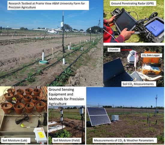
Remote sensing systems used for PA, and agriculture in general, can be classified based on (i) sensor platform and (ii) type of sensor. Sensors are typically mounted on satellites, aerial, and ground-based platforms (Figure 1). Since the 1970s, satellite products have been extensively used for PA. Recently, aerial platforms, which include aircraft and unmanned aerial vehicles (UAVs) are also used in PA. Ground-based platforms used for PA can be grouped into three categories: (i) hand-held, (ii) free standing in the field, and (iii) mounted on tractor or farm machinery. Ground-based systems are also referred to as proximal remote sensing systems because they are located in close proximity to the target surface (land surface or plant) as compared to aerial or satellite-based platforms.
Sensors used for remote sensing differ based on the spatial, spectral, radiometric, and temporal resolution they offer [46]. Spatial resolution of a sensor is defined by the size of the pixel that represents the area on the ground. Sensors with high spatial resolution tend to have small footprints, and sensors with large footprints tend to have a low spatial resolution. Temporal resolution can be considered to be associated with the sensor platform rather than the sensor itself. For example, temporal resolution for a satellite is the time it takes to complete an orbit and revisit the same observation area. Spectral resolution of a sensor is indicated by the number of bands captured in the given range of electromagnetic spectrum [47]. Hyperspectral images contain a large number (10s to 100s) of contagious bands of narrow width (<20 nm) separated by small increments in wavelength [48]. Numerous vegetation indices and statistical and machine learning approaches, such as deep convolutional neural network and random forest, have been applied to reduce the dimensionality of hyperspectral data to extract useful information on crop conditions [49,50,51]. More recently, quantification of solar-induced chlorophyll fluorescence (SIF) from hyperspectral images has increasingly been applied to estimate photosynthesis, plant nutrients, and biotic and abiotic stresses such as disease and water stress [49,50,51,52,53,54].
Although numerous recent satellites provide high spatial (<5 m) and temporal (daily) resolution images, most publicly available satellite products are rather coarse for many PA applications. Appropriate spatio-temporal resolution required for PA depends on several factors including management objectives, size of the field, and the ability of farm equipment to vary the inputs (irrigation, fertilizer, pesticide, etc.) application rates. Crop biomass and yield estimation typically require higher spatial resolution (1–3 m) compared to variable rate fertilizer and irrigation (5–10 m) applications [42]. Furthermore, weed mapping and variable herbicide application require spatial resolution that is finer than the weed patches (e.g., 5–50 cm) [55,56]. Aerial platforms such as UAVs generally provide higher spatial resolution (<5 m) images as compared to the satellites. Thus, UAVs and other ground-based platforms offer greater flexibility in providing images at fine spatial and temporal resolution (more frequent) or as needed.
Sensors mounted on satellites, airplanes, and UAVs are generally passive sensors, i.e., they do not have their own light source. However, some of the satellites have active sensors onboard, such as the active microwave instrument (AMI) on the ERS-1/2. Many of the ground-based remote sensing platforms have active proximity sensors. For example, commercially available variable fertilizer rate application systems such as Green Seeker and Crop Circle have active proximity sensors. In such systems, variations in daylight have minimum effect on measured reflectance, thus providing more accurate and reproducible normalized difference vegetation index (NDVI) or other vegetation indices (VI) used for crop nutrient status assessment.
Two other sensors (thermal infrared and microwave) mounted on recent satellites are increasingly being used in agriculture. Thermal infrared sensors measure energy emitted from a target (e.g., crops) to estimate its temperature, which could be further used to estimate crop water stress, ET, and irrigation requirements [57]. Microwave sensors work in a similar way as the thermal sensors to measure the emitted energy (although in longer microwave wavelengths) from the land surface. Microwave sensors are mainly used to estimate soil moisture contents and crop water use over large areas [58]. Also, microwaves can penetrate through clouds, which is advantageous over other types of sensors that use visible and NIR wavelengths.
However, coarse spatial resolution (10s of km) of the microwave satellite sensors, especially passive sensors, limits their application in PA. Recently, many methods have been developed and used to downscale passive microwave data to a finer resolution for use in PA [59,60,61,62]. Active microwave sensors (e.g., synthetic aperture radar—SAR) generally offer a higher spatial resolution; however, they are also more sensitive to surface roughness (e.g., vegetation) that can introduce errors in soil moisture estimation. Overall, there are a variety of remote sensors and platforms available that can be used to generate high-resolution (spatial, spectral, radiometric, and temporal) images critical to develop and implement site-specific management.
3. Historical Applications of Remote Sensing in Agriculture
Researchers have long recognized the need to map soil and land use databases for sustainable management of natural resources at local, regional, and national scale [63,64]. Knowledge of soil physical, biological, and chemical properties is important to design and implement irrigation, drainage, nutrient, and other crop management strategies, which are essential components of PA. Similarly, land use mapping can help assess the impacts of existing management and policy at regional to national scale. A traditional approach of using remote sensing techniques in agriculture has been around even before 1958, when the term “remote sensing” was first introduced [65]. For example, aerial photography has been used to map soils, land use, and crop conditions in the United States during the 1930 and 1940s [66]. However, these conventional methods of soil mapping and land use classification (e.g., low altitude photography and ground crews) typically involve extensive fieldwork and laboratory analysis, which are expensive and time-consuming [67,68]. Advent of satellite remote sensing during later years facilitated more efficient and effective mapping of land use and land cover at regional, national, and global scales.
Launch of Vanguard 2 and TIROS 1 in 1959 and 1960, respectively, marked the start of satellite remote sensing for meteorological information [69]. However, the era of satellite remote sensing for agriculture started with the launch of Landsat 1 (formerly known as the Earth Resources Technology Satellite—ERTS) on 23 July 1972 by the National Aeronautics and Space Administration (NASA). NASA and the US Department of the Interior through the US Geological Survey (USGS) jointly manage the Landsat program. After Landsat 1, a series of Landsat satellites (Landsat 2–8) were launched to provide high quality images to researchers, land managers, and policy makers to help in the management of natural resources globally (Table 1). Images acquired from Landsat have been used for land use classification, crop classification, and monitoring and irrigation water requirement estimations in many parts of the world [70,71,72,73,74,75]. Later, in 1984, the Landsat 5 Thematic Mapper was launched to collect higher resolution (30 m) images in more bands in visible and NIR region. Currently, the USGS-NASA is planning to launch Landsat 9 (resolution 30 m, 100 m) by mid-2021. In 1986 and 1988, France and India also launched the SPOT 1 and IRS-1A satellites, respectively (Table 1).
Satellite products from these missions were used for land use and crop classification in many large regions of the world. In addition, satellite products are used to monitor soil health, vegetation health, and hydrologic and climatic parameters, which are important for PA (e.g., soil organic carbon, soil moisture, NDVI, leaf area index (LAI), groundwater, and rainfall). Use of the satellite images proved to be cost-effective compared to aerial photography previously used for land use classification over large regions. However, coarse spatiotemporal resolution satellite products are not quite adequate for many PA applications.
Satellites adequate for PA, such as IKONOS, were launched in the late 1990s. IKONOS, launched in 1999, collected imageries at 4-m spatial resolution in visible and NIR bands with a revisit period of up to five days [42]. Imageries collected from IKONOS have been used for multiple purposes in PA, including soil mapping, crop growth and yield prediction, nutrient management, and ET estimation [77,85,86,87]. Launching of numerous nanosatellite constellations during later years addressed further limitations associated with spatial, spectral, and temporal resolution of the satellite imagery [110]. Nanosatellite constellations consist of a large number of small satellites with compact sensors that are cheaper and replaceable [91].
Nanosatellites and other satellites launched after 2000, such as GeoEye-1 (2008), Pleiades-1A (2011), Worldview-3 (2014), SkySat-2 (2014), and Superview-1 (2018), collect multispectral images at a high spatial resolution of ≤2 m with a daily or sub-daily revisit period. Pleiades-1A and Worldview-3 have been used for many PA applications requiring high spatial resolution imagery, including disease and crop water stress detection [118,119,120]. To take advantage of a wide variety of publicly available satellite data, several data fusion approaches have been proposed to combine high/moderate spatial resolution data with high temporal resolution data (and vice-versa) to generate high spatial–temporal resolution data products [121,122]. Satellite data with moderate spatial resolution but high temporal resolution (e.g., Sentinel 2) can also be used with reference ground truth data to help develop PA decision support systems [112].
Despite significant advances in spatial, spectral, and temporal resolution of satellite sensors, the use of satellite images is still limited in commercial agriculture production. Limited flexibility in on-demand imaging solutions, high costs, cloud cover restriction, and lack of automated or established frameworks for image analysis and application are factors affecting large-scale adoption of satellite imageries in PA [123]. These limitations have promoted interest in low-cost proximal remote sensing techniques, including UAVs. Use of UAVs and hand-held, tractor-mounted, and other sensors mounted on farm machinery (e.g., spray boom, fertilizer applicator) has increased tremendously during the last two decades. UAVs with multispectral, hyperspectral, and thermal sensors can provide on-demand information at a spatial scale necessary for PA operations. Getting continuous or frequent satellite scanning during a crop growing season can be problematic due to cloud cover and/or other limitations/uncertainties associated with the sensor platform (e.g., revisit period) [124]. However, UAVs can be flown multiple times during a growing season to acquire information on a cm-scale as required. Most satellites do not offer the data at cm-scale needed for many field-scale PA applications such as weed mapping and disease detection [125,126].
Unprecedented availability of low-cost UAVs is likely to change the face of PA in the future. The average size of a farm in the United States was 179 ha in 2018 [127] and is even smaller in other countries [126]. Acquiring high spatial resolution images obtained from commercial satellites can be expensive, especially for small farms, as many of these images are not available for free. In addition, flying airplanes to obtain such images may be cost-prohibitive for small farms. Images acquired from UAVs offer a low cost alternative to expensive airplane and satellite products [126]. Although the cost of utilizing UAVs (including equipment cost, data processing, and software) at a commercial scale is likely to be a sizable investment for limited resources farmers, continuous development of low-cost sensor technologies and input-production cost savings and/or benefits are likely to outweigh these costs in the future [128,129]. Growth in the development and use of UAVs has enabled the acquisition of high spatial, spectral, and temporal resolution data needed to implement PA management at a crop field or farm scale. Multispectral, high spatial resolution data acquired with UAVs could also be used with available satellite data for scale-up applications over large areas [130].
4. Vegetation Indices
Solar radiation reflected by plants depends on the chemical and morphological characteristics of the plant. Plant type, water content, and canopy characteristics affect the light reflected in each spectral band differently. Measured reflected light in ultraviolet, visible (blue, green, red), and near- and mid-infrared portions of the spectrum has commonly been used to develop various vegetation indices that provide useful information on plant structure and conditions [131] (Table 2). Vegetation indices are mathematical expressions that combine measured reflectance in many spectral bands to produce a value that helps assess crop growth, vigor, and several other vegetation properties such as biomass and chlorophyll content [132]. Mapping of these indices can help understand spatio-temporal variability in crop conditions, which is crucial for PA applications.
Popularly used vegetation indices such as normalized difference vegetation index (NDVI), green NDVI (GNDVI), and soil adjusted vegetation index (SAVI) (Table 2) utilize the fact that within the visible range of spectrum, plant reflectance is low in blue and red regions, while it peaks in the green region (Figure 2). Plant pigments, mainly chlorophyll and carotenoids, adsorb strongly in the visible part of the spectrum except for the green region. However, such strong adsorption does not occur in the NIR part of the spectrum, thus causing high reflectance in NIR region from green and healthy plants (Figure 2). The NDVI uses measured reflectance values in red and NIR regions to provide valuable information on crop growth (LAI, biomass), vigor, and photosynthesis (Table 2). The value of NDVI ranges from −1 to 1, where positive values indicate increasing greenness (LAI and vigor), and negative values indicate non-vegetated surfaces such as urban areas, bare soil/land, water, and ice. External factors to the vegetation conditions such as solar and viewing geometry, soil and crop residue on the land surface, and atmospheric effects may cause interferences in spectral signals [133]. NDVI is sensitive to confounding effects caused due to soils, atmosphere, cloud, and leaf canopy shadow that may result in erroneous information on crop or plant conditions [134,135]. In addition, NDVI is also known to be insensitive to changes in LAI and biomass after reaching a threshold (saturation), especially in dense vegetative conditions [136,137]. A large number of alternative indices have been developed to address these shortcomings in NDVI [135,138,139]. Some of the indices that address these limitations are the soil adjusted vegetation index (SAVI), atmospherically resistant vegetation index (ARVI), and wide dynamic range vegetation index (WDRVI). Red edge based vegetation indices such as red-edge NDVI (RNDVI), normalized difference red edge (NDRE), and red edge difference vegetation index (REDVI) have been shown to perform better than NDVI in estimating plant nutrient status, LAI, and biomass in dense vegetation conditions such as those present during the later growth stages of corn [139,140,141,142].
Measurement of reflectance or emissivity in near- and mid-infrared bands is particularly useful in developing indices that help to understand several intrinsic plant characteristics such as water content, pigments, sugar, carbohydrate, and protein contents [131]. Reflected or emitted radiation in thermal infrared bands is directly related to the plant temperature. Since plant temperature is related to plant transpiration rate, indices obtained from thermal/infrared reflectance data can be used to understand plant water status and other biotic and abiotic stresses such as disease [178,179]. In the past, many indices have been developed based on infrared and thermal reflectance or emission such as crop water stress index (CWSI) and shortwave infrared water stress index (SIWSI; Table 2). These indices have been used for a variety of applications in PA, including water stress and drought monitoring, soil moisture, plant disease, and crop yield estimations [57] (Table 2).
5. Applications
5.1. Irrigation Water Management
Application time and rate of irrigation play an important role in mitigating crop water stress and achieving optimum crop growth and yield. A variety of irrigation management practices are used by farmers depending on many factors including water availability, existing water management infrastructure at the farm (e.g., storage and conveyance system, type of irrigation system), local/regional water laws, economic status, size of the farm, knowledge of farmer, and others [180,181].
Many farmers apply uniform irrigation at regular intervals based on their prior knowledge or experience of farming, soils, and climate at the location [182]. Large commercial farmers deploy soil moisture monitoring systems (wired or wireless moisture sensors) to irrigate (automatically or manually operation mode) based on the measured soil moisture data and crop/plant water requirements [183,184]. Local and regional agricultural agencies may provide irrigation advisory services based on the observed climate and weather conditions in the area [185,186].
Almost all of these conventional farming practices do not consider the variability within a field and use a uniform irrigation rate for the entire field. Remote sensing data can help discern the variability within the field and apply variable rate irrigation with commonly used irrigation systems such as a center pivot. Variable rate application can help mitigate water stress arising from extreme wet and dry conditions to achieve uniformly high yields in all parts in the field while reducing water and nutrient losses [187,188]. Remote sensing images, collected multiple times during a growing season, are used to determine various indicators of crop water demand such as ET, soil moisture, and crop water stress. These indicators are used to estimate crop water requirement and schedule irrigation precisely.
5.1.1. Water Stress
Remote sensing products, either in optical, thermal, and microwave bands, have been used to develop and test multiple indices and techniques for precision water management [189] (Table 2). For example, normalized difference vegetation index (NDVI) and soil adjusted vegetation index (SAVI), developed from optical images, can be used to diagnose water stress and soil moisture conditions for many crops (Table 2). As shown in Table 2, these indices, combined with forecasted weather data, could be used for irrigation scheduling. Thermal remote sensing–based crop water stress index (CWSI) is a popular indicator used to estimate irrigation water demand and scheduling [57].
where Tc is the canopy temperature extracted from thermal images, and Ta is the air temperature. LL and UL indicate the upper and lower limit of the difference in canopy and air temperature. Conceptually, the lower limit (LL) corresponds to the condition when the canopy is transpiring at the potential rate, and the upper limit (UL) corresponds to the condition when transpiration from the canopy is ceased. Multiple methods have been used to calculate the UL and LL of difference in canopy and air temperature, each having their own set of strengths and weaknesses [57]. CWSI has been extensively used for precision irrigation management in orchards [44,190]. For example, Katsigiannis et al. [123] used an autonomous multi-sensor (multi-spectral and thermal sensor) UAV system to develop CWSIs maps for irrigation scheduling and management in kiwi, pomegranate, and vine fields. However, some studies have indicated that more research is needed to establish climate-soil-crop specific trigger/threshold values to enable the use of CWSI for irrigation scheduling [191].
5.1.2. Evapotranspiration (ET)
Evapotranspiration (ET), the largest water flux from the Earth’s surface to the atmosphere, is a critical component of the hydrologic cycle and water balance. Conventional methods of ET measurement (e.g., weighing lysimeter and eddy covariance) are generally expensive and do not provide spatially variable ET estimates resulting from differences in land use, soils, topography and other hydrologic processes [192,193]. Remote sensing data is widely used to estimate ET, which is needed to determine crop water requirements to schedule irrigation [193,194,195]. ET estimation approaches, based on the remote sensing data, can be grouped into three categories: (i) surface energy balance, (ii) crop coefficient, and (iii) the Penman–Monteith method [193,194,196]. Many studies in the past have provided a review of remote-sensing-based ET estimation techniques [39,192,197], including a recent review from Zhang et al. [198] that discussed the theories of development of several ET estimation approaches/methods along with their advantages and limitations. The surface energy balance approach has been extensively used for ET estimation in the past five years. Some of the studies have used hybrid methods to combine crop coefficient and energy balance approaches for ET estimation [195]. In a surface energy balance approach, net radiation flux (Rn), soil heat flux (G), and sensible heat flux (H) are typically calculated from remotely sensed data in visible, near-infrared and thermal infrared bands, while the latent heat flux () is calculated as a reminder of the term in the energy balance equation [195,196].
Recently, Liou and Kar [192] and McShane et al. [197] provided a detailed review of various surface energy balance algorithms used for estimating landscape-scale ET at high spatial resolution and discussed their physical basis, assumptions, uncertainties, and limitations. Surface energy balance techniques use a variety of empirical and physically based models, input data, and assumptions to fully or partially solve the energy balance equation for ET estimation. Popularly used methods such as surface energy balance algorithm for land (SEBAL) and mapping ET at high resolution with internalized calibration (METRIC) fully solve the energy balance equation by determining the sensible heat flux (H) based on the identification of dry and wet pixels in the image [199]. Empirical constants derived from dry and wet pixels and measured radiometric surface temperature are then used to determine pixel-wise surface-air temperature difference and sensible heat-flux. In METRIC, a variant of SEBAL, net radiation is calculated using measured narrowband reflectance and radiometric surface temperature data, while soil heat flux is estimated using net radiation, surface temperature and vegetation indices [197]. Most of the surface energy balance methods typically use similar methods to calculate net radiation and soil heat flux; the major difference lies in the way sensible heat flux is calculated [200]. The primary difference between METRIC and SEBAL is that the METRIC method uses reference ET data calculated from ground-based weather data to calibrate sensible heat and ET estimations obtained from the surface energy balance [199]. Surface energy balance methods are also classified based on the sensible heat sources; two-source energy balance methods account for the individual contributions of soil and vegetation to the total heat flux, while one-source methods do not distinguish between soil and vegetation [195]. Simpler surface energy balance methods, such as simplified surface energy balance index (S-SEBI) and the operational simplified energy balance model (SSEBop) does not require pixel-wise calculation of sensible heat flux and can thus be considered as partial surface energy balance models [199]. Recently, several studies have evaluated these energy balance approaches with satellite data (e.g., Landsat 7 and 8) to estimate ET for irrigation management in PA [201,202,203]. However, coarse spatio-temporal resolution of thermal satellite data limits the application of surface energy balance approaches in PA. More studies are needed to develop and evaluate downscaling techniques that can provide ET estimates at a spatio-temporal resolution necessary for irrigation scheduling in PA.
Crop coefficient based approach for ET estimation involves developing a statistical relationship between a vegetation index (e.g., NDVI, SAVI) and basal crop coefficient (or crop coefficient). A product (ETref*Kc) of reference ET (ETref), estimated from weather data, and crop coefficient (Kc) provides an estimation of potential crop water requirements which can be used in a water balance model to determine irrigation water requirements [122,204,205,206,207]. In the third approach, crop biophysical parameters such as LAI, canopy height, and albedo, estimated from remotely sensed data, are used to determine unknown parameters in Penman-Monteith equation [196,208] for ET estimation. Calculated ET from these approaches is generally used in a soil water balance model to estimate crop irrigation requirements. Bhatti et al. [205] used Landsat 7 and 8 and UAV data to estimate crop coefficient based ET and variable rate irrigation (VRI) requirements for corn and soybean grown in Nebraska, USA. Similarly, Stone et al. [209] demonstrated that variable rate irrigation scheduling based on the NDVI derived crop coefficient and ET can provide corn yields similar to the other precision irrigation techniques relying on measured in-situ soil moisture data. Using crop parameters (LAI and albedo) derived from Sentinel 2A/B images, Bonfante et al. [210] calculated Penman–Monteith ET and time-variable irrigation requirements to demonstrate the application of a publicly available decision support system for maximizing corn yields in Italy.
A large number of approaches exist for ET estimation based on the remote sensing data, each having its own set of advantages and limitations. Some surface energy balance approaches such as S-SEBI do not require any ground-based measurements, and thus, ET can be estimated solely based on the remote sensing data [192]. However, surface energy balance approaches work for only clear sky conditions and suffer from various uncertainties related to the retrieval/estimation of surface temperature, solar parameters, land surface variables (e.g., LAI, vegetation coverage, plant height) and other parameters due to uncertainties in surface emissivity, atmospheric corrections, diurnal variation and aerodynamic surface characteristics [192,198]. In addition, ET estimates derived by solving the surface energy balance equations are instantaneous and require temporal extrapolation to generate daily or larger time step estimates using further assumptions and methods [198]. The Penman–Monteith approach, which uses a process-based model, can provide temporally continuous ET estimations. However, it requires several meteorological parameters that are not easily available at the needed spatio-temporal resolution. Studies have shown that surface energy balance methods such as METRIC and SSEBop provide reasonably accurate (80–95% accuracy) ET estimations on daily to seasonal/annual scales [197]. Generally, ET estimation error of less than 1 mm/day can be considered to be reasonable [211]. However, it also depends on the crop and growth stage; higher accuracies (mm/day) are desirable during initial crop growth stages when ET is lower. However, the accuracy of many of these models (e.g., SEBAL) varies greatly from one spatial and temporal scale to another, making it difficult to quantify the uncertainty in ET estimation [194]. In order to advance the development of remote sensing based ET estimation approaches, further studies are needed to identify and characterize the spatio-temporal structure of uncertainties in the ET estimation due to forcing errors, process errors, and parametrization errors, among others [198]. Advanced approaches that use the knowledge developed from process-based physical models to complement the machine learning based surface energy balance methods need to be explored to develop more accurate and reliable ET estimates at a scale necessary for PA management [212].
5.1.3. Soil Moisture
Remote sensing data acquired in multiple bands, including optical, thermal, and microwave, have been used to estimate soil moisture globally [28,193,213]. Optical and thermal remote sensing data has been extensively used for soil moisture and ET estimations in an approach referred to as “triangle” or “trapezoid” or land surface temperature-vegetation index (LST-VI) method [198,214,215,216]. The triangle or LST-VI method is based on the physical relationship between the land surface temperature (and thus soil moisture and latent heat fluxes) and vegetative cover characteristics. Soil moisture estimation in this method is based on the interpretation of the pixel distribution in the LST-VI plot-space. If a sufficiently large number of pixels are present in an image covering a full range of soil moisture and vegetation density and when cloud, surface water, and other outliers are removed, the LST-VI space resembles a triangle or trapezoid [214]. One edge of the LST-VI triangle or trapezoid falling toward higher temperatures represent dry edge (low soil moisture), while the opposite side represents the wet edge (high soil moisture) [217]. Triangular or trapezoidal shape of the LST-VI space is formed due to the low sensitivity of LST to soil moisture under dense vegetative conditions, which is contrary to the high sensitivity of LST to soil moisture under bare soil or sparse vegetation conditions. Once upper and lower limit moisture content for wet and dry edges is determined, theoretically, soil moisture for remaining pixels can be estimated using interpolation techniques. The triangle method uses a simple parametrization approach and does not require ancillary atmospheric or surface data for soil moisture estimation [214,218]. However, a subjective determination of wet and dry edges in the triangle method can introduce significant uncertainties in soil moisture estimation especially over relatively homogenous land-surface areas (e.g., rainfed agriculture during dry season) and after rainfall events when there is a general lack of variability in soil moisture to form an LST-VI triangle [215]. In addition, the traditional triangle method requires individual parametrization for each observation date, which is a time-consuming and computationally demanding process [60]. The traditional triangle method also needs both optical and thermal data that may not be available in certain instances (e.g., Sentinel-2).
Recently, a newer generation of triangular models has been developed and tested for high spatial resolution mapping of soil moisture in PA applications [59,60]. One such technique, called the optical trapezoid model (OPTRAM), replaces the LST in the traditional triangle model with short-wave-infra-red transformed reflectance (STR). Analogous to the traditional triangle model, soil moisture in OPTRAM is estimated based on the interpretation of STR-VI space [60]. Using Sentinel-2 and Landsat-8 data, Sadeghi et al. [53] showed reasonably accurate (<0.04 cm3/cm3) soil moisture estimations with OPTRAM model for grass and cropland dominated watersheds in Arizona and Oklahoma, USA. The OPTRAM model does not require thermal remote sensing data, thus making it more suitable for a wide range of remote sensing data. Unlike LST, surface reflectance (STR) is a function of surface properties and does not vary significantly with ambient atmospheric conditions, which eliminates the need to parametrize/calibrate the model for individual dates [216]. However, compared to the traditional triangle model, the OPTRAM model is more sensitive to saturated land areas, which may result in increased uncertainty in soil moisture estimates [60]. More studies are needed to further evaluate these newer models for their applicability in a diverse range of climatic, hydrologic, and environmental conditions.
Compared to the data acquired in visible, NIR, and SWIR bands, microwave remote sensing data have a greater potential to provide accurate soil moisture estimations [216]. Signals in visible and NIR regions have weaker penetration ability, compared to microwave, and is more likely to get affected by interferences caused due to atmospheric and cloud conditions [135]. Microwave sensors measure dielectric properties of soil based on land surface emissivity or scattering for soil moisture estimation. Several satellites with active and passive microwave sensors have been launched for soil moisture monitoring such as the advanced microwave scanning radiometer-earth observing system (AMSR-E), soil moisture and ocean salinity (SMOS), soil moisture active passive (SMAP), and Sentinel-1 [216].
Active microwave sensors provide higher spatial resolution as compared to the passive sensors. However, active sensors also suffer from measurement uncertainties caused due to land surface roughness and vegetative cover or canopy [219]. On the other hand, although passive sensors are more accurate and provide better temporal resolution, they also provide a coarser spatial resolution (e.g., 10s of km) [215]. Typically, watershed and regional scale hydrologic and agricultural applications, especially PA, require finer resolution data [220].
Several spatial downscaling techniques have been developed and used in the past to address the coarse spatial resolution limitation of passive microwave sensors. These techniques can be broadly categorized into two main groups: (i) satellite-based methods and (ii) modeling methods [221]. Typically, satellite-based methods use vegetation, surface temperature, and other geophysical and environmental information obtained from high spatial resolution satellite data (in optical and thermal bands) to downscale coarse resolution soil moisture data [61,62].
Machine learning and data mining techniques have been used with topography, land surface temperature, albedo, land cover, NDVI, and ET obtained from high spatial resolution satellite data to downscale coarse resolution soil moisture data from passive microwave sensors [135,222]. Higher resolution (1 km) land surface temperature and vegetation data derived from moderate resolution imaging spectroradiometer (MODIS) have popularly been used in many studies to downscale coarse resolution soil moisture data [135,223,224]. Many others have used higher spatial resolution backscatter data from active microwave sensors to disaggregate and downscale brightness and soil moisture data from passive sensors [225]. Some studies have used a combination of SAR (Sentinel 1/2) and optical remote sensing data with machine learning techniques to downscale passive microwave (e.g., SMAP) data [226,227]. Modeling-based methods use high spatial resolution data derived from physically-based and statistical models with data assimilation approaches to downscale coarse-resolution soil moisture data [221,228]. Despite the development of these downscaling techniques, spatio-temporal resolution of soil moisture estimates generated from microwave data is still coarse and/or lacks the accuracy needed for PA, limiting their application for irrigation scheduling in PA. Recent launches of multi-polarization sensors (e.g., Radarsat-2) along with the development of new polarization parameters and polarization decomposition methods can potentially help generating soil moisture and crop information at higher spatial resolution [229]. Multi-polarization SAR data can be combined with optical satellite data to generate soil moisture estimates at high spatial resolution [230]. Further efforts are needed to develop advanced downscaling techniques that can combine data from multiple sources (e.g., optical and microwave remote sensing, biophysical and hydrologic models) and provide temporally continuous (e.g., daily) soil moisture estimates at the finer spatial resolution necessary for PA [221]. Overall, in addition to satellites, high spatial resolution data acquired from UAVs in optical, thermal, infrared, and microwave bands carry great promise for soil moisture mapping and other PA applications [231,232,233].
5.2. Nutrient Management
Timely and appropriate application of fertilizers is essential to optimize crop growth and yields while minimizing environmental damage through nutrient losses to groundwater and surface water. Typically, a recommended rate of fertilizer is uniformly applied during planting and later crop growth stages. However, the fertilizer requirement of crops varies spatially and temporally (during and among seasons) due to differences in soils, management, topography, weather, and hydrology [12,234]. Mapping of such variability in crop nutrient status/requirement for PA applications could be challenging with conventionally used tools such as chlorophyll meters [165].
Several vegetation indices (e.g., NDVI, SAVI), derived from remote sensing data, have been shown to be significantly correlated with plant chlorophyll content, photosynthetic activity, and plant productivity (Table 2). Mapping of these indices can thus help understand the spatial variability in crop nutrient status, which is important for PA. Recently, several tractor mounted remote sensors have become available that can measure plant nutrient status for real-time application of spatially-variable fertilizer rates. Green Seeker, Yara N-sensor, and Crop Circle are some examples of commercially available hand-held and tractor mounted remote sensors that use crop reflectance data to determine and apply spatially variable fertilizer rates in real-time [235].
In tractor mounted systems, remote sensors are usually mounted ahead of the spray boom. Nitrogen (N) application rates in these systems are determined based on the calculated vegetation indices (e.g., NDVI), which are further communicated to nutrient applicator/spreader for real-time fertilizer application. Different algorithms are used to convert the measured vegetation indices into recommended N-application rates. In general, the N-application rates are calculated by comparing measured vegetation indices in the target field with a reference vegetation index measured in a well fertilized (N-rich) plot/strip that is representative of the target field. Several fertilizer rate calculation algorithms (e.g., the nitrogen fertilizer optimization algorithm) [236,237] have been developed and successfully implemented in these commercially available sensors to determine vegetation-indices based in-season N-requirements for many crops [238,239].
Despite the commercialization of variable rate N-management technologies based on proximal remote sensing, farmer’s adoption remains low in many agricultural enterprises [240]. A lack of clear evidence on significant economic benefits (crop yield and/or profits), especially in commercial farm settings (i.e., large fields) is a limiting factor for the large scale adoption of these technologies [241]. To further refine these remote sensing based technologies and enhance its benefits, research is being conducted with UAVs and other remote sensors for a variety of crops in different climatic regions. Maresma et al. [165] used images captured from a UAV to determine the suitability of several vegetation indices and crop height in determining in-season fertilizer application rates for corn grown in Spain. Cao et al. [242] showed that Green Seeker and Crop Circle sensors resulted in reduced N-fertilizer use and increased N-productivity for winter wheat production in China. Overall, remote sensing based mapping of crop nutrient status in PA can help increase crop nutrient use efficiency while maintaining/increasing crop yields and reducing off-site nutrient losses that are damaging to the environment.
Remote sensing has also been used to determine soil organic matter and phosphorus content to develop spatial maps that can aid in site-specific management [243,244,245,246]. Blasch et al. [243] used multi-temporal satellite images from RapidEye in conjunction with principal component analysis to develop field-scale soil organic matter maps to aid in site-specific precision management. Castaldi et al. [245] used images obtained from Sentinel-2 to develop soil organic carbon maps at both field and regional scales in Germany, Luxembourg, and Belgium and showed that the satellite data have an adequate spatial resolution for field scale planning in PA management. Crop growth is a function of several biotic and abiotic factors related to soils, management, topography, hydrology, and other environmental variables. Therefore, vegetation indices derived from remote sensing of crop growth/status are reflective of the combined variability in these factors or stressors. While using the vegetation indices to determine the plant nutrient status or N-application rates, one should also consider potentially confounding effects caused due to other stressors such as moisture stress and disease.
5.3. Disease Management
Diseases can cause a significant loss of crop production and farm profits. Early detection of plant disease and its spatial extent can help contain the disease spread and reduce production losses. Field scouting, a conventional method of disease detection, is time consuming, labor intensive, and prone to human error [126]. In addition, with field scouting, it may be difficult to detect the disease during the early stages when the symptoms are not fully visible. Furthermore, some diseases do not show any visible symptoms, or the effect may not be noticeable until it is too late to act [247]. It is also difficult to map the spatial extent and severity of the disease spread with the traditional method of field scouting.
Remote sensing could be used to monitor the disease efficiently, especially in the early stages of disease development, when it may be difficult to discern the signs of disease with field scouting. Multiple techniques using RGB, multi-spectral, hyperspectral, thermal, and fluorescence imaging have been used to identify diseases in a variety of crops [178]. Di Gennaro et al. [248] found a good correlation between grapevine leaf stripe disease and NDVI generated from UAV imageries in Italy. Abdulridha et al. [172] used a machine learning approach with vegetation indices derived from hyperspectral UAV images to detect citrus canker with 96% accuracy even during the early stage of disease development. As the differences in spectral signatures observed in a field can occur due to a combination of biotic and abiotic stresses, it could be challenging to discern the effects caused due to individual stressors (e.g., disease, water or nutrient stress). As compared to the typically used vegetation indices (e.g., NDVI), the development of disease specific spectral disease indices (SDI) can increase the accuracy of disease detection and differentiation under real world field conditions [249,250]. Higher disease detection accuracies during critical crop growth stages such as flowering can help implement effective management plans in a timely manner to mitigate or avoid large yield and fruit quality losses. Use of SDIs, in place of typical VIs, can also reduce the complexity of disease detection methods and increase the system efficacy by reducing the computational demand [250]. Although studies have been conducted for plant disease classification [251], further efforts are needed to develop more accurate, automated and reproducible methodologies for disease detection under diverse climatic and real-world field conditions [40].
5.4. Weed Management
Conventional weed management approaches involving a uniform application of herbicide is an inefficient practice that increases the risk for off-site pesticide losses [252]. Application of herbicide at a variable rate as per need can help enhance the treatment efficiency and reduce input costs and environmental pollution [253]. Remote sensing has widely been used for mapping weed patches in crop fields for site-specific weed management [43]. Weeds can be identified or differentiated from crop plants based on their peculiar spectral signature related to their phenological or morphological attributes that are different from the crop. Over the last few years, machine learning approaches have emerged as a highly accurate and efficient method of image classification for weed mapping [254,255,256]. Two general types of image classification approaches are commonly used for weed mapping; supervised and unsupervised classification. Although each method has its own strengths and weaknesses, supervised classification is time-intensive and requires more manual work [26].
UAVs have been the most popular remote sensing platform for weed mapping and management primarily due to its capability to produce cm-scale resolution (5 cm) [257]) images needed for weed detection and mapping. Using the fully convolutional network approach, Huang et al. [254] mapped weeds in a rice field in China with up to 90% accuracy. Partel et al. [255] developed a target weed sprayer using deep learning neural network approach for ground-sensor based weed detection that yielded in 71% application accuracy in experimental fields in Florida, USA. However, the commercial adoption of these technologies remains challenging, given the expertise required to use advanced software and technical processes involved in their applications [258].
5.5. Crop Monitoring and Yield
Monitoring crop growth and yield are necessary to understand the crop response to the environment and agronomic practices and develop effective management plans for fieldwork and/or remedies [259]. LAI and biomass are two essential indicators of crop health and development [28]. LAI is also used as an input in many crop growth and yield forecasting models [260]. In-situ methods of LAI estimation (physical and optical) are time consuming and labor intensive, similar to the destructive field methods used for biomass estimation. Also, these methods do not provide a spatial variability map of crop growth and biomass [261,262]. Remote sensing data on crop growth (e.g., LAI) and biomass can help obtain valuable information on site-specific properties (e.g., soils, topography), management (e.g., water, nutrient, and other inputs), and various biotic and abiotic stressors (e.g., diseases, weeds, water, and nutrient stress) [263]. Similarly, remote sensing data can also be used to map differences in tillage and residue management and its effects on crop growth [264]. Several studies have used hyperspectral images with various machine learning and classification techniques to map tillage and crop residue in agricultural fields [265,266]. Such information on crop conditions and tillage practices can help develop site specific management plans, including variable water, nutrient, and pesticide application to increase production and management efficiency.
Remote sensing data have been used to estimate LAI and biomass for a variety of crops, including row crops, orchards, and vine crops [267,268,269]. Typically, such studies use a set of reference data (e.g., measured LAI and corresponding vegetation indices) to develop a regression or machine learning based approach to estimate LAI and/or biomass for a target field. Yue et al. [262] used multiple spectral indices in conjunction with measured plant height to estimate biomass (R2 = 0.74) in multiple irrigations and nutrient treatment plots for winter wheat grown in China. Ali et al. [269] used red-edge position (REP) extracted from hyperspectral images to predict LAI (R2 = 0.93) and chlorophyll content (R2 = 0.90) for Kinnow mandarins grown in Pakistan. REP is the position of the main inflection point of the red-NIR slope created due to strong chlorophyll absorption in the red spectrum and canopy scattering in the NIR region [269]. Reliable LAI estimation from reflectance data could be difficult, especially during early crop growth stages due to interference from the bare soil surface. To overcome this limitation, modified vegetation indices adjusted for soil and other interferences have been proposed and used to estimate LAI [270]. Recently, red-edge based vegetation indices have been shown to be promising for estimating LAI in multiple crops [271].
For PA, knowledge of spatial variability in crop yield is important to understand crop response to management practices and environmental stressors. Remote sensing derived crop biophysical parameters, or vegetation indices have a strong correlation with observed crop yield and biomass, indicating their potential for use in yield estimation [259]. Crop yield estimation from remotely sensed data has generally been conducted in two ways.
First, biophysical parameters (e.g., LAI) derived from remotely sensed data are used in a crop model to estimate the crop yield and biomass. Second, statistical (e.g., regression) or empirical relationships are developed between remote sensing derived crop parameters/indices (e.g., NDVI, LAI) and observed crop yield and biomass in a representative crop field. The developed regression model or empirical relationship could then be used to map crop yield at a target crop field. Crop modeling is a data-intensive approach, which requires a large amount of information as model input parameters, meteorological data, and observed yield and biomass data.
Maresma et al. [161] used a regression based approach to evaluate the relationship between corn yield and biomass and spectral indices measured at the V12 stage. Similar to other studies, they also found that the red-based indices NDVI and wide dynamic range vegetation index (WDRVI) had the highest correlation with grain yields for a range of fertilizer application rates. Spatial mapping of crop biophysical parameters or indices at multiple times during a growing season is likely to provide a better estimation of crop biomass and yield as compared to a single snapshot during the season [263].
6. Progress Made, Needs, and Challenges
Remote sensing has potential applications in almost every aspect of PA, from land preparation to harvesting. The abundance of high spatial resolution multi-temporal satellite data along with low-cost UAVs and commercially available ground-based proximity sensors have changed the face of PA. A large number of advanced techniques, including empirical, regression, and various forms of machine learning approaches have been used to explore the potential applications of remote sensing in PA. Similarly, many vegetation indices have been developed and tested for their ability to help PA operations, including variable fertilizer management, irrigation scheduling, disease control, weed mapping, and yield forecasting. However, many challenges need to be addressed before the remote sensing technologies can potentially see a large-scale adoption in commercial and non-commercial agriculture.
Although most of the satellite data are available for free, it may require a significant amount of technical knowledge and expertise to process them for real-world applications. For example, image pre-processing and post-processing require expert knowledge and software. In addition, many PA operations such as disease and weed management require fine spatial resolution (cm-scale) data with high spectral and temporal (e.g., daily) resolution. Most of the publicly available satellite data do not meet such requirements. Furthermore, cloudy days and variable or inconsistent irradiance or sunlight may render many satellite images unsuitable for use.
Users/farmers may need to purchase high resolution (spatial, temporal and spectral) satellite data, which can be cost-prohibitive, especially for small farms. However, images acquired from UAVs are likely to offer a low-cost alternative for small farm operations [272]. Use of UAVs and tractor-mounted sensors also involve the use of special software for data analysis and need professional operators (e.g., drone licensing) [235]. Hyperspectral images acquired from the state of the art sensors mounted on some of the recently launched satellites and UAVs provide a large amount of information on crop biophysical parameters. However, these sensors are expensive (UAVs), and the processing of imageries is complex [246]. There is a need to explore and develop advanced information and communication technologies as well as chemometric and spectral decomposition methods to synthesize and generate practical information needed for PA applications. Artificial intelligence techniques, including machine learning, has great potential to generate spatially and temporally continuous information from instantaneous satellite data at a scale necessary for many PA applications [212]. Hybrid methods, combining the knowledge obtained from physically based models, can complement such AI techniques to help develop techniques useful in PA decision making [43,212].
Despite a large number of studies on remote sensing applications in PA, there is a general lack of established techniques and/or framework that are accurate, reproducible, and applicable under a wide variety of climatic, soil, crop, and management conditions. Accuracies of methods using remote sensing (satellite, aerial, and UAV) data depends on a variety of factors including image resolution (spatial, spectral, and temporal); atmospheric, climatic, and weather conditions; crop and field conditions (e.g., growth stage, land cover); and the analyses technique (e.g., regression-based, machine learning, physically based modeling). For example, the accuracy of surface energy balance techniques for ET estimation varies significantly in space and time, causing a large uncertainty in PA decision making. More studies are needed to understand the spatio-temporal structure of uncertainty in estimating ET, soil moisture, disease stress, and other crop parameters. Spectral signature from a crop is a reflection of crop status/response to site characteristics (e.g., soil, topography), management, and simultaneously acting multiple biotic and abiotic stressors (e.g., diseases, weeds, nutrient and water stress, etc.). A disease detection method found suitable under controlled experimental conditions may not perform similarly well in real-world conditions where multiple biotic and biotic stressors govern crop response or conditions. Given the complexity of image processing methods and the amount of technical knowledge and expertise it requires for application, there is a need to explore and develop a simple and reliable workflow for image pre-processing, analysis and application in real time. Major challenges and gaps remain in the development of tools and frameworks that can facilitate the use of satellite data for real-time applications by the end-users. Development of accurate, user-friendly systems is likely to result in wider adoption of remote sensing data in commercial and non-commercial PA operations.
Author Contributions
R.P.S., R.L.R., and S.K.S. developed this concept, including method and approach to be used; R.P.S. and R.L.R. outlined the manuscript. R.P.S. and R.L.R. reviewed remotely sensed data; S.K.S. contributed to the discussion of this manuscript. All authors have read and agreed to the published version of the manuscript.
Funding
This research was funded by the United States Department of Agriculture (USDA) National Institute of Food and Agriculture (NIFA), Evans–Allen project 1004053.
Acknowledgments
This work was supported by the Evans–Allen project of the United States Department of Agriculture (USDA), National Institute of Food and Agriculture. We thank Richard McWhorter, Samiksha Ray, and Tosin Kayode for their time to edit this paper.
Conflicts of Interest
The authors declare no conflict of interest.
References
- Awokuse, T.O.; Xie, R. Does agriculture really matter for economic growth in developing countries? Can. J. Agric. Econ. 2015, 63, 77–99. [Google Scholar]
- Gillespie, S.; Van den Bold, M. Agriculture, food systems, and nutrition: Meeting the challenge. Glob. Chall. 2017, 1, 1600002. [Google Scholar]
- Patel, R. The long green revolution. J. Peasant Stud. 2013, 40, 1–63. [Google Scholar]
- Pingali, P.L. Green revolution: Impacts, limits, and the path ahead. Proc. Natl. Acad. Sci. USA 2012, 109, 12302–12308. [Google Scholar]
- Wik, M.; Pingali, P.; Broca, S. Background Paper for the World Development Report 2008: Global Agricultural Performance: Past Trends and Future Prospects; World Bank: Washington, DC, USA, 2008. [Google Scholar]
- World Bank Group. Available online: https://openknowledge.worldbank.org/handle/10986/9122 (accessed on 21 May 2020).
- Konikow, L.F. Long-term groundwater depletion in the United States. Groundwater 2015, 53, 2–9. [Google Scholar]
- Kleinman, P.J.; Sharpley, A.N.; McDowell, R.W.; Flaten, D.N.; Buda, A.R.; Tao, L.; Bergstrom, L.; Zhu, Q. Managing agricultural phosphorus for water quality protection: Principles for progress. Plant Soil 2011, 349, 169–182. [Google Scholar]
- Wen, F.; Chen, X. Evaluation of the impact of groundwater irrigation on streamflow in Nebraska. J. Hydrol. 2006, 327, 603–617. [Google Scholar]
- Konikow, L.F.; Kendy, E. Groundwater depletion: A global problem. Hydrogeol. J. 2005, 13, 317–320. [Google Scholar]
- Sishodia, R.P.; Shukla, S.; Graham, W.D.; Wani, S.P.; Jones, J.W.; Heaney, J. Current, and future groundwater withdrawals: Effects, management and energy policy options for a semi-arid Indian watershed. Adv. Water Resour. 2017, 110, 459–475. [Google Scholar]
- Hendricks, G.S.; Shukla, S.; Roka, F.M.; Sishodia, R.P.; Obreza, T.A.; Hochmuth, G.J.; Colee, J. Economic and environmental consequences of overfertilization under extreme weather conditions. J. Soil Water Conserv. 2019, 74, 160–171. [Google Scholar]
- Delgado, J.; Short, N.M.; Roberts, D.P.; Vandenberg, B. Big data analysis for sustainable agriculture. FSUFS 2019, 3, 54. [Google Scholar]
- Berry, J.K.; Delgado, J.A.; Khosla, R.; Pierce, F.J. Precision conservation for environmental sustainability. J. Soil Water Conserv. 2003, 58, 332–339. [Google Scholar]
- Srinivasan, A. (Ed.) Handbook of Precision Agriculture: Principles and Applications; Food Products Press, Haworth Press Inc.: New York, NY, USA, 2006; ISBN 13:978-1-56022-955-1. [Google Scholar]
- Aubert, B.A.; Schroeder, A.; Grimaudo, J. IT as enabler of sustainable farming: An empirical analysis of farmers’ adoption decision of precision agriculture technology. Decis. Support Syst. 2012, 54, 510–520. [Google Scholar] [CrossRef] [Green Version]
- Pierpaolia, E.; Carlia, G.; Pignattia, E.; Canavaria, M. Drivers of precision agriculture technologies adoption: A literature review. Proc. Technol. 2013, 8, 61–69. [Google Scholar] [CrossRef] [Green Version]
- Gebbers, R.; Adamchuk, V. Precision agriculture and food security. Science 2010, 327, 828–831. [Google Scholar] [CrossRef]
- Zhang, N.; Wang, M.; Wang, N. Precision agriculture—A worldwide overview. Comput. Electron. Agric. 2002, 36, 113–132. [Google Scholar] [CrossRef]
- Bongiovanni, R.; Lowenberg-DeBoer, J. Precision agriculture and sustainability. Precis. Agric. 2004, 5, 359–387. [Google Scholar] [CrossRef]
- Koch, B.; Khosla, R.; Frasier, W.M.; Westfall, D.G.; Inman, D. Economic feasibility of variable-rate nitrogen application utilizing site-specific management zones. Agron. J. 2004, 96, 1572–1580. [Google Scholar] [CrossRef] [Green Version]
- Hedley, C. The role of precision agriculture for improved nutrient management on farms. J. Sci. Food Agric. 2014, 95, 12–19. [Google Scholar] [CrossRef]
- Boursianis, A.D.; Papadopoulou, M.S.; Diamantoulakis, P.; Liopa-Tsakalidi, A.; Barouchas, P.; Salahas, G.; Karagiannidis, G.; Wan, S.; Goudos, S.K. Internet of Things (IoT) and Agricultural Unmanned Aerial Vehicles (UAVs) in smart farming: A comprehensive review. IEEE Internet Things 2020. [Google Scholar] [CrossRef]
- Jha, K.; Doshi, A.; Patel, P.; Shah, M. A comprehensive review on automation in agriculture using artificial intelligence. Artif. Intell. Agric. 2019, 2, 1–12. [Google Scholar] [CrossRef]
- Elijah, O.; Rahman, T.A.; Orikumhi, I.; Leow, C.Y.; Hindia, M.N. An overview of Internet of Things (IoT) and data analytics in agriculture: Benefits and challenges. IEEE Internet Things 2018, 5, 3758–3773. [Google Scholar] [CrossRef]
- Huang, Y.; Chen, Z.; Yu, T.; Huang, X.; Gu, X. Agricultural remote sensing big data: Management and applications. J. Integr. Agric. 2018, 7, 1915–1931. [Google Scholar] [CrossRef]
- Kamilaris, A.; Kartakoullis, A.; Prenafeta-Boldú, F.X. A review on the practice of big data analysis in agriculture. Comput. Electron. Agric. 2017, 143, 23–37. [Google Scholar] [CrossRef]
- Zhou, L.; Chen, N.; Chen, Z.; Xing, C. ROSCC: An efficient remote sensing observation-sharing method based on cloud computing for soil moisture mapping in precision agriculture. IEEE J. Sel. Top. Appl. Earth Obs. Remote Sens. 2016, 9, 5588–5598. [Google Scholar] [CrossRef]
- Khattab, A.; Abdelgawad, A.; Yelmarthi, K. Design and implementation of a cloud-based IoT scheme for precision agriculture. In Proceedings of the 2016 28th International Conference on Microelectronics (ICM), Giza, Egypt, 17 December 2016; Volume 4, pp. 201–204. [Google Scholar]
- Pavo’n-Pulido, N.; Lo’pez-Riquelme, J.A.; Torres, R.; Morais, R.; Pastor, J.A. New trends in precision agriculture: A novel cloud-based system for enabling data storage and agricultural task planning and automation. Precis. Agric. 2017, 18, 1038–1068. [Google Scholar] [CrossRef]
- Say, M.S.; Keskin, M.; Sehri, M.; Sekerli, Y.E. Adoption of precision agriculture technologies in developed and developing countries. TOJSAT 2018, 8, 7–15. [Google Scholar]
- Rokhmana, C.A. The potential of UAV-based remote sensing for supporting precision agriculture in Indonesia. Proc. Environ. Sci. 2015, 24, 245–253. [Google Scholar] [CrossRef] [Green Version]
- Chivasa, W.; Mutanga, O.; Biradar, C. Application of remote sensing in estimating maize grain yield in heterogeneous African agricultural landscapes: A review. Int. J. Remote Sens. Appl. 2017, 38, 6816–6845. [Google Scholar] [CrossRef]
- Schellberg, J.; Hill, M.J.; Gerhards, R.; Rothmund, M.; Braun, M. Precision agriculture on grassland: Applications, perspectives and constraints. Eur. J. Agron. 2008, 29, 59–71. [Google Scholar] [CrossRef]
- Maia, R.F.; Netto, I.; Tran, A.L.H. Precision agriculture using remote monitoring systems in Brazil. In Proceedings of the 2017 IEEE Global Humanitarian Technology Conference (GHTC), San Jose, CA, USA, 19 October 2017; pp. 1–6. [Google Scholar]
- Borgogno-Mondino, E.; Lessio, A.; Tarricone, L.; Novello, V.; Palma, D.L. A comparison between multispectral aerial and satellite imagery in precision viticulture. Precis. Agric. 2018, 19, 195–217. [Google Scholar] [CrossRef]
- Ge, Y.; Thomasson, J.A.; Sui, R. Remote sensing of soil properties in precision agriculture: A review. Front. Earth Sci. 2011, 5, 229–238. [Google Scholar] [CrossRef]
- Courault, D.; Seguin, B.; Olioso, A. Review on estimation of evapotranspiration from remote sensing data: From empirical to numerical modeling approaches. Irrig. Drain. Syst. 2005, 19, 223–249. [Google Scholar] [CrossRef]
- Maes, W.H.; Steppe, K. Estimating evapotranspiration and drought stress with ground-based thermal remote sensing in agriculture: A review. J. Exp. Bot. 2012, 63, 4671–4712. [Google Scholar] [CrossRef] [Green Version]
- Zhang, J.; Huang, Y.; Pu, R.; Gonzalez-Moreno, P.; Yuan, L.; Wu, K.; Huang, W. Monitoring plant diseases and pests through remote sensing technology: A review. Comput. Electron. Agric. 2019, 165, 104943. [Google Scholar] [CrossRef]
- Atzberger, C. Advances in remote sensing of agriculture: Context description, existing operational monitoring systems and major information needs. Remote Sens. Environ. 2013, 5, 949–981. [Google Scholar] [CrossRef] [Green Version]
- Mulla, D.J. Twenty-five years of remote sensing in precision agriculture: Key advances and remaining knowledge gaps. Biosyst. Eng. 2013, 114, 358–371. [Google Scholar] [CrossRef]
- Weiss, M.; Jacob, F.; Duveillerc, G. Remote sensing for agricultural applications: A meta-review. Remote Sens. Environ. 2020, 236, 111402. [Google Scholar] [CrossRef]
- Maes, W.H.; Steppe, K. Perspectives for remote sensing with unmanned aerial vehicles in precision agriculture. Trends Plant Sci. 2019, 24, 152–154. [Google Scholar] [CrossRef]
- Angelopoulou, T.; Tziolas, N.; Balafoutis, A.; Zalidis, G.; Bochtis, D. Remote sensing techniques for soil organic carbon estimation: A review. Remote Sens. 2019, 11, 676. [Google Scholar] [CrossRef] [Green Version]
- Santosh, K.M.; Sundaresan, J.; Roggem, R.; Déri, A.; Singh, R.P. Geospatial Technologies and Climate Change; Springer International Publishing: Dordrecht, The Netherlands, 2014. [Google Scholar]
- Nowatzki, J.; Andres, R.; Kyllo, K. Agricultural Remote Sensing Basics. NDSU Extension Service Publication. 2004. Available online: www.ag.ndsu.nodak.edu (accessed on 23 September 2020).
- Teke, M.; Deveci, H.S.; Haliloğlu, O.; Gürbüz, S.Z.; Sakarya, U. A short survey of hyperspectral remote sensing applications in agriculture. In Proceedings of the 2013 6th International Conference on Recent Advances in Space Technologies (RAST), Istanbul, Turkey, 12 June 2013; pp. 171–176. [Google Scholar]
- Chang, C.Y.; Zhou, R.; Kira, O.; Marri, S.; Skovira, J.; Gu, L.; Sun, Y. An Unmanned Aerial System (UAS) for concurrent measurements of solar induced chlorophyll fluorescence and hyperspectral reflectance toward improving crop monitoring. Agric. For. Meteorol. 2020, 294, 1–15. [Google Scholar] [CrossRef]
- Nagasubramanian, K.; Jones, S.; Singh, A.K.; Sarkar, S.; Singh, A.; Ganapathysubramanian, B. Plant disease identifcation using explainable 3D deep learning on hyperspectral images. Plant Methods 2019, 15, 1–10. [Google Scholar] [CrossRef]
- Chlingaryan, A.; Sukkarieh, S.; Whelan, B. Machine learning approaches for crop yield prediction and nitrogen status estimation in precision agriculture: A review. Comput. Electron. Agric. 2018, 151, 61–69. [Google Scholar] [CrossRef]
- Camino, C.; González-Dugo, V.; Hernández, P.; Sillero, J.C.; Zarco-Tejada, P.J. Improved nitrogen retrievals with airborne-derived fluorescence and plant traits quantified from VNIR-SWIR hyperspectral imagery in the context of precision agriculture. Int. J. Appl. Earth Obs. Geoinf. 2018, 70, 105–117. [Google Scholar] [CrossRef]
- Zarco-Tejada, P.J.; González-Dugo, M.V.; Fereres, E. Seasonal stability of chlorophyll fluorescence quantified from airborne hyperspectral imagery as an indicator of net photosynthesis in the context of precision agriculture. Remote Sens. Environ. 2016, 179, 89–103. [Google Scholar] [CrossRef]
- Mohammed, G.H.; Colombo, R.; Middleton, E.M.; Rascher, U.; van der Tole, C.; Nedbald, L.; Goulas, Y.; Pérez-Priego, O.; Damm, A.; Meroni, M.; et al. Remote sensing of solar-induced chlorophyll fluorescence (SIF) in vegetation: 50 years of progress. Remote Sens. Environ. 2019, 231, 1–39. [Google Scholar]
- Fernández-Quintanilla, C.; Peña, J.M.; Andújar, D.; Dorado, J.; Ribeiro, A.; López-Granados, F. Is the current state of the art of weed monitoring suitable for site-specific weed management in arable crops? Weed Res. 2018, 58, 259–272. [Google Scholar]
- Castaldi, F.F.; Pelosi, F.; Pascucci, S.; Casa, R. Assessing the potential of images from unmanned aerial vehicles (UAV) to support herbicide patch spraying in maize. Precis. Agric. 2017, 18, 76–94. [Google Scholar]
- Khanal, S.; Fulton, J.; Shearer, S. An overview of current and potential applications of thermal remote sensing in precision agriculture. Comput. Electron. Agric. 2017, 139, 22–32. [Google Scholar]
- Palazzi, V.; Bonafoni, S.; Alimenti, F.; Mezzanotte, P.; Roselli, L. Feeding the world with microwaves: How remote and wireless sensing can help precision agriculture. IEEE Microw. Mag. 2019, 20, 72–86. [Google Scholar]
- Babaeian, E.; Sidike, P.; Newcomb, M.S.; Maimaitijiang, M.; White, S.A.; Demieville, J.; Ward, R.W.; Sadeghi, M.; LeBauer, D.S.; Jones, S.B.; et al. A new optical remote sensing technique for high resolution mapping of soil moisture. Front. Big Data 2019, 2, 37. [Google Scholar] [CrossRef] [Green Version]
- Sadeghi, M.; Babaeian, E.; Tuller, M.; Jones, S.B. The optical trapezoid model: A novel approach to remote sensing of soil moisture applied to Sentinel-2 and Landsat-8 observations. Remote Sens. Environ. 2017, 198, 52–68. [Google Scholar] [CrossRef] [Green Version]
- Fang, B.; Lakshmi, V.; Bindlish, R.; Jackson, T.J. AMSR2 soil moisture downscaling using temperature and vegetation data. Remote Sens. 2018, 10, 1575. [Google Scholar] [CrossRef] [Green Version]
- Im, J.; Park, S.; Rhee, J.; Baik, J.; Choi, M. Downscaling of AMSR-E soil moisture with MODIS products using machine learning approaches. Environ. Earth Sci. 2016, 75, 1–19. [Google Scholar]
- Pereira, P.; Brevik, E.; Muñoz-Rojas, M.; Miller, B. Soil Mapping and Process Modeling for Sustainable Land Use Management; Elsevier: Amsterdam, The Netherlands, 2017. [Google Scholar]
- Metternicht, G. Land Use and Spatial Planning: Enabling Sustainable Management of Land Resources; Springer: New York, NY, USA, 2018. [Google Scholar]
- Nellis, M.D.; Price, K.P.; Rundquist, D. Remote sensing of cropland agriculture. In The SAGE Handbook of Remote Sensing; Sage: London, UK, 2009; Volume 1, pp. 368–380. [Google Scholar]
- With, K.A. Essential of Landscape Ecology; Oxford University Press: Oxford, UK, 2019. [Google Scholar]
- Forkuor, G.; Hounkpatin, O.K.L.; Welp, G.; Thiel, M. High resolution mapping of soil properties using remote sensing variables in southwestern burkina faso: A comparison of machine learning and multiple linear regression models. PLoS ONE 2017, 12, e0170478. [Google Scholar] [CrossRef]
- Still, D.A.; Shih, S.F. Using Landsat data to classify land use for assessing the basinwide runoff index 1. J. Am. Water Resour. Assoc. 1985, 21, 931–940. [Google Scholar] [CrossRef]
- Kidder, S.Q.; Kidder, R.M.; Haar, T.H.V. Satellite Meteorology: An Introduction; Academic Press: San Diago, CA, USA, 1995; p. 466. [Google Scholar]
- Odenyo, V.A.O.; Pettry, D.E. Land-use mapping by machine processing of Landsat-1 data. PERS 1977, 43, 515–523. [Google Scholar]
- Welch, R.; Pannell, C.W.; Lo, C.P. Land use in Northeast China, 1973: A view from Landsat-1. AAAG 1975, 65, 595–596. [Google Scholar] [CrossRef]
- Kirchhof, W.; Haberäcker, P.; Krauth, E.; Kritikos, G.; Winter, R. Evaluation of Landsat image data for land-use mapping. Acta Astronaut. 1980, 7, 243–253. [Google Scholar] [CrossRef]
- Blair, B.; Baumgardner, M.F. Detection of the green and brown wave in hardwood canopy covers using multidate, multispectral data from Landsat-11. Agron J. 1977, 69, 808–811. [Google Scholar] [CrossRef]
- Bauer, M.E.; Cipra, J.E.; Anuta, P.E.; Etheridge, J.B. Identification and area estimation of agricultural crops by computer classification of Landsat MSS data. Remote Sens. Environ. 1979, 8, 77–92. [Google Scholar] [CrossRef]
- Estes, J.E.; Jensen, J.R.; Tinney, L.R. Remote sensing of agricultural water demand information: A California study. Water Resour. Res. 1978, 14, 170–176. [Google Scholar] [CrossRef]
- Leslie, C.R.; Serbina, L.O.; Miller, H.M. Landsat and Agriculture—Case Studies on the Uses and Benefits of Landsat Imagery in Agricultural Monitoring and Production; US Geological Survey Open-File Report; US Geological Survey: Reston, VA, USA, 2017; Volume 1034, p. 27.
- Seelan, S.K.; Laguette, S.; Casady, G.M.; Seielstad, G.A. Remote sensing applications for precision agriculture: A learning community approach. Remote Sens. Environ. 2003, 88, 157–169. [Google Scholar] [CrossRef]
- Scudiero, E.; Corwin, D.L.; Wienhold, B.J.; Bosley, B.; Shanahan, J.F.; Johnson, C.K. Downscaling Landsat 7 canopy reflectance employing a multi-soil sensor platform. Precis. Agric. 2016, 17, 53–73. [Google Scholar] [CrossRef]
- Venancio, L.P.; Mantovani, E.C.; do Amaral, C.H.; Neale, C.M.U.; Gonçalves, I.Z.; Filgueiras, R.; Campos, I. Forecasting corn yield at the farm level in Brazil based on the FAO-66 approach and soil-adjusted vegetation index (SAVI). Agric. Water Manag. 2019, 225, 105779. [Google Scholar] [CrossRef]
- Dong, T.; Liu, J.; Qian, B.; Zhao, T.; Jing, Q.; Geng, X.; Wang, J.; Huffman, T.; Shang, J. Estimating winter wheat biomass by assimilating leaf area index derived from fusion of Landsat-8 and MODIS data. Int. J. Appl. Earth Obs. Geoinf. 2016, 49, 63–74. [Google Scholar] [CrossRef]
- Worsley, P.; Bowler, J. Assessing flood damage using SPOT and NOAA AVHRR data. Geospat. Inf. Agric. 2001, 2–7. Available online: http://www.regional.org.au/au/gia/12/397worsley.htm#TopOfPage (accessed on 23 September 2020).
- Mondal, P.; Basu, M. Adoption of precision agriculture technologies in India and in some developing countries: Scope, present status and strategies. Prog. Nat. Sci. 2009, 19, 659–666. [Google Scholar] [CrossRef]
- Koenig, K.; Höfle, B.; Hämmerle, M.; Jarmer, T.; Siegmann, B.; Lilienthal, H. Comparative classification analysis of post-harvest growth detection from terrestrial LiDAR point clouds in precision agriculture. ISPRS J. Photogramm. Remote Sens. 2015, 104, 112–125. [Google Scholar] [CrossRef]
- McNairn, H.; Ellis, J.; Van Der Sanden, J.J.; Hirose, T.; Brown, R.J. Providing crop information using RADARSAT-1 and satellite optical imagery. ISPRS J. Photogramm. Remote Sens. 2002, 23, 851–870. [Google Scholar] [CrossRef]
- Enclona, E.A.; Thenkabail, P.S.; Celis, D.; Diekmann, J. Within-field wheat yield prediction from IKONOS data: A new matrix approach. ISPRS J. Photogramm. Remote Sens. 2004, 25, 377–388. [Google Scholar] [CrossRef]
- Sullivan, D.G.; Shaw, J.N.; Rickman, D. IKONOS imagery to estimate surface soil property variability in two alabama physiographies. Soil Sci. Soc. Am. J. 2005, 69, 1789–1798. [Google Scholar]
- Yang, G.; Pu, R.; Zhao, C.; Xue, X. Estimating high spatiotemporal resolution evapotranspiration over a winter wheat field using an IKONOS image based complementary relationship and Lysimeter observation. Agric. Water Manag. 2014, 133, 34–43. [Google Scholar] [CrossRef]
- Omran, E.E. Remote estimation of vegetation parameters using narrow band sensor for precision agriculture in arid environment. Egypt. J. Soil Sci. 2018, 58, 73–92. [Google Scholar] [CrossRef] [Green Version]
- Apan, A.; Held, A.; Phinn, S.; Markley, J. Detecting sugarcane ‘orange rust’ disease using EO-1 Hyperion hyperspectral imagery. Int. J. Remote Sens. 2004, 25, 489–498. [Google Scholar]
- Filippi, P.; Jones, J.E.; Niranjan, S.; Wimalathunge, N.S.; Somarathna, D.S.N.P.; Liana, E.; Pozza, L.E.; Ugbaje, S.U.; Jephcott, T.G.; Paterson, S.E.; et al. An approach to forecast grain crop yield using multi-layered, multi-farm data sets and machine learning. Precis. Agric. 2019, 20, 1–16. [Google Scholar]
- Houborg, R.; McCabe, M.F. High-resolution NDVI from planet’s constellation of Earth observing nanosatellites: A new data source for precision agriculture. Remote Sens. 2016, 8, 768. [Google Scholar]
- Mobasheri, M.R.; Jokar, J.; Ziaeian, P.; Chahardoli, M. On the methods of sugarcane water stress detection using Terra/ASTER images. Am. Eurasian J. Agric. Environ. Sci. 2007, 2, 619–627. [Google Scholar]
- Santoso, H.; Gunawan, T.; Jatmiko, R.H.; Darmosarkoro, W.; Minasny, B. Mapping and identifying basal stem rot disease in oil palms in North Sumatra with QuickBird imagery. Precis. Agric. 2011, 12, 233–248. [Google Scholar]
- Jackson, T.J.; Bindlish, R.; Klein, M.; Gasiewski, A.J.; Njoku, E.G. Soil moisture retrieval and AMSR-E validation using an airborne microwave radiometer in SMEX02. In Proceedings of the 2003 IEEE International Geoscience and Remote Sensing Symposium, Toulouse, France, 21–25 July 2003; Volume 1, pp. 401–403. [Google Scholar]
- Yang, C.; Everitt, J.H.; Bradford, J.M. Evaluating high resolution SPOT 5 satellite imagery to estimate crop yield. Precis. Agric. 2009, 10, 292–303. [Google Scholar]
- Sai, M.S.; Rao, P.N. Utilization of resourcesat-1 data for improved crop discrimination. Int. J. Appl. Earth Obs. Geoinf. 2008, 10, 206–210. [Google Scholar]
- Lee, J.W.; Park, G.; Joh, H.K.; Lee, K.H.; Na, S.I.; Park, J.H.; Kim, S.J. Analysis of relationship between vegetation indices and crop yield using KOMPSAT (KoreaMulti-Purpose SATellite)-2 imagery and field investigation data. JKSAE 2011, 53, 75–82. [Google Scholar]
- Gao, S.; Niu, Z.; Huang, N.; Hou, X. Estimating the Leaf Area Index, height and biomass of maize using HJ-1 and RADARSAT-2. Int. J. Appl. Earth Obs. Geoinf. 2013, 24, 1–18. [Google Scholar]
- Siegfried, J.; Longchamps, L.; Khosla, R. Multisectral satellite imagery to quantify in-field soil moisture variability. J. Soil Water Conserv. 2019, 74, 33–40. [Google Scholar]
- De Lara, A.; Longchamps, L.; Khosla, R. Soil water content and high-resolution imagery for precision irrigation: Maize yield. Agron. J. 2019, 9, 174. [Google Scholar]
- Shang, J.; Liu, J.; Ma, B.; Zhao, T.; Jiao, X.; Geng, X.; Huffman, T.; Kovacs, J.M.; Walters, D. Mapping spatial variability of crop growth conditions using RapidEye data in Northern Ontario, Canada. Remote Sens. Environ. 2015, 168, 113–125. [Google Scholar]
- Caturegli, L.; Casucci, M.; Lulli, F.; Grossi, N.; Gaetani, M.; Magni, S.; Bonari, E.; Volterrani, M. GeoEye-1 satellite versus ground-based multispectral data for estimating nitrogen status of turfgrasses. Int. J. Remote Sens. 2015, 36, 2238–2251. [Google Scholar]
- Tian, J.; Wang, L.; Li, X.; Gong, H.; Shi, C.; Zhong, R.; Liu, X. Comparison of UAV and WorldView-2 imagery for mapping leaf area index of mangrove forest. Int. J. Appl. Earth Obs. Geoinf. 2017, 61, 22–31. [Google Scholar]
- Kokhan, S.; Vostokov, A. Using vegetative indices to quantify agricultural crop characteristics. Ecol. Eng. 2020, 21, 122–129. [Google Scholar] [CrossRef]
- Romanko, M. Remote Sensing in Precision Agriculture: Monitoring Plant Chlorophyll, and Soil Ammonia, Nitrate, and Phosphate in Corn and Soybean Fields. Ph.D. Thesis, Bowling Green State University, Bowling Green, OH, USA, 2017. [Google Scholar]
- Skakun, S.; Justice, C.O.; Vermote, E.; Roger, J.C. Transitioning from MODIS to VIIRS: An analysis of inter-consistency of NDVI data sets for agricultural monitoring. Int. J. Remote Sens. 2018, 39, 971–992. [Google Scholar] [PubMed]
- Kim, S.J.; Lee, M.S.; Kim, S.H.; Park, G. Potential application topics of kompsat-3 image in the field of precision agriculture model. Korean Soc. Remote Sens. 2006, 48, 17–22. [Google Scholar]
- Yuan, L.; Pu, R.; Zhang, J.; Wang, J.; Yang, H. Using high spatial resolution satellite imagery for mapping powdery mildew at a regional scale. Precis. Agric. 2016, 17, 332–348. [Google Scholar] [CrossRef]
- Ferguson, R.; Rundquist, D. Remote sensing for site-specific crop management. Precis. Agric. Basics 2018. [Google Scholar] [CrossRef]
- Sidike, P.; Sagan, V.; Maimaitijiang, M.; Maimaitiyiming, M.; Shakoor, N.; Burken, J.; Fritschi, F.B. dPEN: Deep progressively expanded network for mapping heterogeneous agricultural landscape using WorldView-3 satellite imagery. Remote Sens. Environ. 2018, 221, 756–772. [Google Scholar] [CrossRef]
- Martínez-Casasnovas, J.A.; Uribeetxebarría, A.; Escolà, A.; Arnó, J. Sentinel-2 vegetation indices and apparent electrical conductivity to predict barley (Hordeum vulgare L.) yield. In Precision Agriculture; Wageningen Academic Publishers: Wageningen, The Netherlands, 2019; pp. 415–421. [Google Scholar]
- Wolters, S.; Söderström, M.; Piikki, K.; Stenberg, M. Near-real time winter wheat N uptake from a combination of proximal and remote optical measurements: How to refine Sentinel-2 satellite images for use in a precision agriculture decision support system. In Proceedings of the 12th European Conference on Precision Agriculture, Montpellier, France, 8–11 July 2019; Wageningen Academic Publishers: Wageningen, The Netherlands, 2019; pp. 415–421. [Google Scholar]
- Bajwa, S.G.; Rupe, J.C.; Mason, J. Soybean disease monitoring with leaf reflectance. Remote Sens. 2017, 9, 127. [Google Scholar] [CrossRef] [Green Version]
- El Sharif, H.; Wang, J.; Georgakakos, A.P. Modeling regional crop yield and irrigation demand using SMAP type of soil moisture data. J. Hydrometeorol. 2015, 16, 904–916. [Google Scholar] [CrossRef]
- Hao, Z.; Zhao, H.; Zhang, C.; Wang, H.; Jiang, Y. Detecting winter wheat irrigation signals using SMAP gridded soil moisture data. Remote Sens. 2019, 11, 2390. [Google Scholar] [CrossRef] [Green Version]
- Chua, R.; Qingbin, X.; Bo, Y. Crop Monitoring Using Multispectral Optical Satellite Imagery. Available online: https://www.21at.sg/publication/publication/cotton-crop-monitoring-using-multispectral-optical-satellite-ima/ (accessed on 23 September 2020).
- Fisher, J.B.; Lee, B.; Purdy, A.J.; Halverson, G.H.; Dohlen, M.B.; Cawse-Nicholson, K.; Wang, A.; Anderson, R.G.; Aragon, B.; Arain, M.A.; et al. ECOSTRESS: NASA’s next generation mission to measure evapotranspiration from the international space station. Water Resour. Res. 2020, 56, e2019WR026058. [Google Scholar] [CrossRef]
- Navrozidisa, I.; Alexandridisa, T.K.; Dimitrakosb, A.; Lagopodic, A.L.; Moshoud, D.; Zalidisa, G. Identification of purple spot disease on asparagus crops across spatial and spectral scales. Comput. Electron. Agric. 2018, 148, 322–329. [Google Scholar] [CrossRef] [Green Version]
- Bannari, A.; Mohamed, A.M.A.; El-Battay, A. Water stress detection as an indicator of red palm weevil attack using worldview-3 data. In Proceedings of the 2017 IEEE International Geoscience and Remote Sensing Symposium (IGARSS), Fort Worth, TX, USA, 23 July 2017; pp. 4000–4003. [Google Scholar]
- Salgadoe, A.S.A.; Robson, A.J.; Lamb, D.W.; Dann, E.K.; Searle, C. Quantifying the severity of phytophthora root rot disease in avocado trees using image analysis. Remote Sens. 2018, 10, 226. [Google Scholar] [CrossRef] [Green Version]
- Zhu, X.; Cai, F.; Tian, J.; Williams, T.K.A. Spatiotemporal fusion of multisource remote sensing data: Literature survey, taxonomy, principles, applications, and future directions. Remote Sens. 2018, 10, 527. [Google Scholar]
- Knipper, K.R.; Kustas, W.P.; Anderson, M.C.; Alfieri, J.G.; Prueger, J.H.; Hain, C.R.; Gao, F.; Yang, Y.; McKee, L.G.; Nieto, H.; et al. Evapotranspiration estimates derived using thermal-based satellite remote sensing and data fusion for irrigation management in California vineyards. Irrig. Sci. 2019, 37, 431–449. [Google Scholar] [CrossRef]
- Katsigiannis, P.; Galanis, G.; Dimitrakos, A.; Tsakiridis, N.; Kalopesas, C.; Alexandridis, T.; Chouzouri, A.; Patakas, A.; Zalidis, G. Fusion of spatio-temporal UAV and proximal sensing data for an agricultural decision support system. In Proceedings of the Fourth International Conference on Remote Sensing and Geoinformation of the Environment RSCy 2016, Paphos, Cyprus, 12 August 2016; Volume 9688, p. 96881R. [Google Scholar]
- Primicerio, J.; Di Gennaro, S.F.; Fiorillo, E.; Genesio, L.; Lugato, E.; Matese, A.; Vaccar, F.P. A flexible unmanned aerial vehicle for precision agriculture. Precis. Agric. 2012, 13, 517–523. [Google Scholar] [CrossRef]
- Huang, W.; Lu, J.; Ye, H.; Kong, W.A.; Mortimer, H.; Shi, Y. Quantitative identification of crop disease and nitrogen-water stress in winter wheat using continuous wavelet analysis. Int. J. Agric. Biol. Eng. 2018, 11, 145–151. [Google Scholar] [CrossRef] [Green Version]
- Ehsani, R.; Maja, J.M. The rise of small UAVs in precision agriculture. Resour. Mag. 2013, 20, 18–19. [Google Scholar]
- USDA. Farms and Land in Farms: 2017 Summary. United States Department of Agriculture (USDA); National Agricultural Statistics Service: Washington, DC, USA, 2019; p. 19.
- Honrado, J.L.E.; Solpico, D.B.; Favila, C.M.; Tongson, E.; Tangonan, G.L.; Libatique, N.J.C. UAV Imaging with low-cost multispectral imaging system for precision agriculture applications. In Proceedings of the 2017 IEEE Global Humanitarian Technology Conference (GHTC), San Jose, CA, USA, 19 October 2017. [Google Scholar]
- Abdullahi, H.S.; Mahieddine, F.; Sheriff, R.E. Technology impact on agricultural productivity: A review of precision agriculture using unmanned aerial vehicles. In Proceedings of the International Conference on Wireless and Satellite Systems; Springer: Cham, Switzerland, 2015; pp. 388–400. [Google Scholar]
- Zhang, S.; Zhao, G.; Lang, K.; Su, B.; Chen, X.; Xi, X.; Zhang, H. Integrated satellite, Unmanned Aerial Vehicle (UAV) and ground inversion of the SPAD of winter wheat in the reviving stage. Sensors 2019, 19, 1485. [Google Scholar] [CrossRef] [Green Version]
- Xue, J.; Su, B. Significant remote sensing vegetation indices: A review of developments and application. J. Sens. 2017. [Google Scholar] [CrossRef] [Green Version]
- McKinnon, T.; Hoff, P. Comparing RGB-based vegetation indices with NDVI for drone based agricultural sensing. AGBX 2017, 021, 1–8. Available online: https://agribotix.com/wp-content/uploads/2017/05/Agribotix-VARI-TGI-Study.pdf (accessed on 23 September 2020).
- Rondeaux, G.; Steven, M.; Baret, F. Optimization of soil-adjusted vegetation indices. Remote Sens. Environ. 1996, 55, 95–107. [Google Scholar] [CrossRef]
- Carlson, T.N.; Ripley, D.A. On the relation between NDVI, fractional vegetation cover, and leaf area index. Remote Sens. Environ. 1997, 62, 241–252. [Google Scholar] [CrossRef]
- Chen, S.; She, D.; Zhang, L.; Guo, M.; Liu, X. Spatial downscaling methods of soil moisture based on multisource remote sensing data and its application. Water 2019, 11, 1401. [Google Scholar]
- Hashimoto, N.; Saito, Y.; Maki, M.; Homma, K. Simulation of reflectance and vegetation indices for Unmanned Aerial Vehicle (UAV) monitoring of paddy fields. Remote Sens. 2019, 11, 2119. [Google Scholar]
- Tan, C.; Zhang, P.; Zhou, X.; Wang, Z.; Xu, Z.; Mao, W.; Li, W.; Huo, Z.; Guo, W.; Yun, F. Quantitative monitoring of leaf area index in wheat of different plant types by integrating nDVi and Beer-Lambert law. Sci. Rep. 2020, 10, 929. [Google Scholar]
- Sun, Y.; Ren, H.; Zhang, T.; Zhang, C.; Qin, Q. Crop leaf area index retrieval based on inverted difference vegetation index and NDVI. IEEE Geosci. Remote 2018, 15, 1662–1666. [Google Scholar]
- LI, F.; Miao, Y.; Feng, G.; Yuan, F.; Yue, S.; Gao, X.; Liu, Y.; Liu, B.; Ustin, S.L.; Chen, X. Improving estimation of summer maize nitrogen status with red edge-based spectral vegetation indices. Field Crops Res. 2014, 157, 111–123. [Google Scholar]
- Shaver, T.M.; Kruger, G.R.; Rudnick, D.R. Crop canopy sensor orientation for late season nitrogen determination in corn. J. Plant Nutr. 2017, 40, 2217–2223. [Google Scholar]
- Xie, Q.; Dash, J.; Huang, W.; Peng, D.; Qin, Q.; Mortimer, H.; Casa, R.; Pignatti, S.; Laneve, G.; Pascucci, S.; et al. Vegetation indices combining the red and red-edge spectral information for leaf area index retrieval. IEEE J. Sel. Top. Appl. Earth Obs. Remote Sens. 2018, 11, 1482–1493. [Google Scholar]
- Lu, J.; Miao, Y.; Huang, Y.; Shi, W.; Hu, X.; Wang, X.; Wan, J. Evaluating an Unmanned Aerial Vehicle-based Remote Sensing System for Estimation of Rice Nitrogen Status. In Proceedings of the Fourth International Conference on Agro-Geoinformatics (Agro-geoinformatics), Istanbul, Turkey, 20 July 2015; pp. 198–203. [Google Scholar]
- Govaerts, B.; Verhulst, N. The Normalized Difference Vegetation Index (NDVI) GreenSeekerTM Handheld Sensor: Toward the Integrated Evaluation of Crop Management; CIMMYT: Mexico City, Mexico, 2010; p. 13. [Google Scholar]
- Schaefer, M.T.; Lamb, D.W. A combination of plant NDVI and LiDAR measurements improve the estimation of pasture biomass in tall fescue (Festuca arundinacea var. Fletcher). Remote Sens. 2016, 8, 109. [Google Scholar]
- Duan, T.; Chapman, S.C.; Guo, Y.; Zheng, B. Dynamic monitoring of NDVI in wheat agronomy and breeding trials using an unmanned aerial vehicle. Field Crops Res. 2017, 210, 71–80. [Google Scholar]
- Hassan, M.A.; Yang, M.; Rasheed, A.; Yang, G.; Reynolds, M.; Xia, X.; Xiao, Y.; He, Z. A rapid monitoring of NDVI across the wheat growth cycle for grain yield prediction using a multi-spectral UAV platform. Plant Sci. 2019, 282, 95–103. [Google Scholar]
- Amaral, L.R.; Molin, J.P.; Portz, G.; Finazzi, F.B.; Cortinov, L. Comparison of crop canopy reflectance sensors used to identify sugarcane biomass and nitrogen status. Precis. Agric. 2015, 16, 15–28. [Google Scholar] [CrossRef]
- Ihuoma, S.O.; Madramootoo, C.A. Sensitivity of spectral vegetation indices for monitoring water stress in tomato plants. Comput. Electron. Agric. 2019, 163, 104860. [Google Scholar] [CrossRef]
- Ballester, C.; Zarco-Tejada, P.J.; Nicolás, E.; Alarcón, J.J.; Fereres, E.; Intrigliolo, D.S.; Gonzalez-Dugo, V.J.P.A. Evaluating the performance of xanthophyll, chlorophyll and structure-sensitive spectral indices to detect water stress in five fruit tree species. Precis. Agric. 2018, 19, 178–193. [Google Scholar] [CrossRef]
- Zhou, J.; Khot, L.R.; Boydston, R.A.; Miklas, P.N.; Porter, L. Low altitude remote sensing technologies for crop stress monitoring: A case study on spatial and temporal monitoring of irrigated pinto bean. Precis. Agric. 2018, 19, 555–569. [Google Scholar]
- Cao, Q.; Miao, Y.; Shen, J.; Yu, W.; Yuan, F.; Cheng, S.; Huang, S.; Wang, H.; Yang, W.; Liu, F. Improving in-season estimation of rice yield potential and responsiveness to topdressing nitrogen application with Crop Circle active crop canopy sensor. Precis. Agric. 2016, 17, 136–154. [Google Scholar] [CrossRef]
- Lukas, V.; Novák, J.; Neudert, L.; Svobodova, I.; Rodriguez-Moreno, F.; Edrees, M.; Kren, J. The combination of UAV survey and landsat imagery for monitoring of crop vigor in precision agriculture. In The International Archives of the Photogrammetry, Remote Sensing and Spatial Information Sciences, Proceedings of the 2016 XXIII ISPRS Congress, Prague, Czech Republic, 12–19 July 2016; Available online: https://www.int-arch-photogramm-remote-sens-spatial-inf-sci.net/XLI-B8/953/2016/ (accessed on 23 September 2020). [CrossRef]
- Khan, M.S.; Semwal, M.; Sharma, A.; Verma, R.K. An artificial neural network model for estimating Mentha crop biomass yield using Landsat 8 OLI. Precis. Agric. 2020, 21, 18–33. [Google Scholar]
- Pourazar, H.; Samadzadegan, F.; Javan, F.D. Aerial multispectral imagery for plant disease detection: Radiometric calibration necessity assessment. Eur. J. Remote Sens. 2019, 52, 17–31. [Google Scholar]
- Kanke, Y.; Tubana, B.; Dalen, M.; Harrell, D. Evaluation of red and red-edge reflectance-based vegetation indices for rice biomass and grain yield prediction models in paddy fields. Precis. Agric. 2016, 17, 507–530. [Google Scholar] [CrossRef]
- DadrasJavan, F.; Samadzadegan, F.; Pourazar, S.H.S.; Fazeli, H. UAV-based multispectral imagery for fast Citrus Greening detection. J. Plant Dis. Protect. 2019, 126, 307–318. [Google Scholar] [CrossRef]
- Phadikar, S.; Goswami, J. Vegetation indices based segmentation for automatic classification of brown spot and blast diseases of rice. In Proceedings of the 3rd International Conference on Recent Advances in Information Technology (RAIT), Dhanbad, India, 3 March 2016; pp. 284–289. [Google Scholar]
- Marino, S.; Cocozza, C.; Tognetti, R.; Alvino, A. Use of proximal sensing and vegetation indexes to detect the inefficient spatial allocation of drip irrigation in a spot area of tomato field crop. Precis. Agric. 2015, 16, 613–629. [Google Scholar] [CrossRef]
- Ranjan, R.; Chandel, A.K.; Khot, L.R.; Bahlol, H.Y.; Zhou, J.; Boydston, R.A.; Miklas, P.N. Irrigated pinto bean crop stress and yield assessment using ground based low altitude remote sensing technology. Inf. Process. Agric. 2019, 6, 502–514. [Google Scholar] [CrossRef]
- Tahir, M.N.; Naqvi, S.Z.A.; Lan, Y.; Zhang, Y.; Wang, Y.; Afzal, M.; Cheema, M.J.M.; Amir, S. Real time estimation of chlorophyll content based on vegetation indices derived from multispectral UAV in the kinnow orchard. IJPAA 2018. [Google Scholar] [CrossRef] [Green Version]
- Maresma, Á.; Ariza, M.; Martínez, E.; Lloveras, J.; Martínez-Casasnovas, J.A. Analysis of vegetation indices to determine nitrogen application and yield prediction in maize (Zea mays L.) from a standard UAV service. Remote Sens. 2016, 8, 973. [Google Scholar]
- Towers, P.C.; Strever, A.; Poblete-Echeverría, C. Comparison of vegetation indices for leaf area index estimation in vertical shoot positioned vine canopies with and without grenbiule hail-protection netting. Remote Sens. 2019, 11, 1073. [Google Scholar]
- Mudereri, B.T.; Dube, T.; Adel-Rahman, E.M.; Niassy, S.; Kimathi, E.; Khan, Z.; Landmann, T. A comparative analysis of PlanetScope and Sentinel-2 space-borne sensors in mapping Striga weed using Guided Regularised Random Forest classification ensemble. Int. Arch. Photogramm. Remote Sens. Spat. Inf. Sci. 2019, 42, 701–708. [Google Scholar]
- Khosravirad, M.; Omid, M.; Sarmadian, F.; Hosseinpour, S. Predicting sugarcane yields in khuzestan using a large time-series of remote sensing imagery region. Int. Arch. Photogramm. Remote Sens. Spat. Inf. Sci. 2019, 42, 645–648. [Google Scholar] [CrossRef] [Green Version]
- Marino, S.; Alvino, A. Hyperspectral vegetation indices for predicting onion (Allium cepa L.) yield spatial variability. Comput. Electron. Agric. 2015, 116, 109–117. [Google Scholar] [CrossRef]
- Das, P.K.; Laxman, B.; Rao, S.K.; Seshasai, M.V.R.; Dadhwal, V.K. Monitoring of bacterial leaf blight in rice using ground-based hyperspectral and LISS IV satellite data in Kurnool, Andhra Pradesh, India. Int. J. Pest Manag. 2015, 61, 359–368. [Google Scholar] [CrossRef]
- Zhang, P.; Zhou, X.; Wang, Z.; Mao, W.; Li, W.; Yun, F.; Guo, W.; Tan, C. Using HJ-ccD image and pLS algorithm to estimate the yield of field-grown winter wheat. Sci. Rep. 2020, 10, 5173. [Google Scholar] [CrossRef] [Green Version]
- Klem, K.; Záhora, J.; Zemek, F.; Trunda, P.; Tůma, I.; Novotná, K.; Hodaňová, P.; Rapantová, B.; Hanuš, J.; Vavříková, J.; et al. Interactive effects of water deficit and nitrogen nutrition on winter wheat. Remote sensing methods for their detection. Agric. Water Manag. 2018, 210, 171–184. [Google Scholar]
- Liu, P.; Shi, R.; Gao, W. Estimating leaf chlorophyll contents by combining multiple spectral indices with an artificial neural network. Earth Sci. Inf. 2018, 11, 147–156. [Google Scholar]
- Meng, J.; Xu, J.; You, X. Optimizing soybean harvest date using HJ-1 satellite imagery. Precis. Agric. 2015, 16, 164–179. [Google Scholar]
- Taskos, D.G.; Koundouras, S.; Stamatiadis, S.; Zioziou, E.; Nikolaou, N.; Karakioulakis, K.; Theodorou, N. Using active canopy sensors and chlorophyll meters to estimate grapevine nitrogen status and productivity. Precis. Agric. 2015, 16, 77–98. [Google Scholar]
- Abdulridha, J.; Ampatzidis, Y.; Kakarla, S.C.; Roberts, P. Detection of target spot and bacterial spot diseases in tomato using UAV-based and benchtop-based hyperspectral imaging techniques. Precis. Agric. 2019, 21, 955–978. [Google Scholar]
- Rapaport, T.; Hochberg, U.; Cochavi, A.; Karnieli, A.; Rachmilevitch, S. The potential of the spectral ‘water balance index’(WABI) for crop irrigation scheduling. New Phytol. 2017, 216, 741–757. [Google Scholar] [PubMed] [Green Version]
- Gao, Y.; Walker, J.P.; Allahmoradi, M.; Monerris, A.; Ryu, D.; Jackson, T.J. Optical sensing of vegetation water content: A synthesis study. IEEE J. STARS 2015, 8, 1456–1464. [Google Scholar]
- Ma, B.; Pu, R.; Zhang, S.; Wu, L. Spectral identification of stress types for maize seedlings under single and combined stresses. IEEE Access 2018, 6, 13773–13782. [Google Scholar]
- DeJonge, K.C.; Taghvaeian, S.; Trout, T.J.; Comas, L.H. Comparison of canopy temperature-based water stress indices for maize. Agric. Water Manag. 2015, 156, 51–62. [Google Scholar]
- Kullberg, E.G.; DeJonge, K.C.; Chávez, J.L. Evaluation of thermal remote sensing indices to estimate crop evapotranspiration coefficients. Agric. Water Manag. 2017, 179, 64–73. [Google Scholar]
- Mahlein, A.K. Plant disease detection by imaging sensors–parallels and specific demands for precision agriculture and plant phenotyping. Plant Dis. 2016, 100, 241–251. [Google Scholar]
- Prashar, A.; Jones, H.G. Assessing drought responses using thermal infrared imaging. In Environmental Responses in Plants; Humana Press: New York, NY, USA, 2016; pp. 209–219. [Google Scholar]
- Uphoff, N. Improving International Irrigation Management with Farmer Participation: Getting the Process Right; Routledge: London, UK, 2018. [Google Scholar]
- Pardossi, A.; Incrocci, L.; Incrocci, G.; Malorgio, F.; Battista, P.; Bacci, L.; Rapi, B.; Marzialetti, P.; Hemming, J.; Balendonck, J. Root zone sensors for irrigation management in intensive agriculture. Sensors 2009, 9, 2809–2835. [Google Scholar] [CrossRef] [PubMed] [Green Version]
- Boland, A.; Bewsell, D.; Kaine, G. Adoption of sustainable irrigation management practices by stone and pome fruit growers in the Goulburn/Murray Valleys. Aust. Irrig. Sci. 2006, 24, 137–145. [Google Scholar] [CrossRef]
- Thompson, R.B.; Gallardo, M.; Valdez, L.C.; Fernadez, M.D. Using plant water status to define threshold values for irrigation management of vegetable crops using moisture sensors. Agric. Water Manag. 2007, 88, 147–158. [Google Scholar] [CrossRef]
- Holt, N.; Sishodia, R.P.; Shukla, S.; Hansen, K.M. Improved water and economic sustainability with low-input compact bed plasticulture and precision irrigation. J. Irrig. Drain. Eng. 2019, 145, 04019013. [Google Scholar] [CrossRef]
- Eching, S. Role of technology in irrigation advisory services: The CIMIS experience. In Proceedings of the 18th Congress and 53rd IEC meeting of the International Commission on Irrigation and Drainage (ICID), FAO/ICID International Workshop on Irrigation Advisory Services and Participatory Extension Management, Montreal, QC, Canada, 24 July 2002; Volume 24. Available online: http://www.ipcinfo.org/fileadmin/user_upload/faowater/docs/ias/paper24.pdf (accessed on 23 September 2020).
- Smith, M.; Munoz, G. Irrigation advisory services for effective water use: A review of experiences. In Proceedings of the Irrigation Advisory Services and Participatory Extension in Irrigation Management Workshop Organized by FAO-ICID, Montreal, QC, Canada, 24 July 2002. [Google Scholar]
- Evans, R.G.; LaRue, J.; Stone, K.C.; King, B.A. Adoption of site-specific variable rate sprinkler irrigation systems. Irrig. Sci. 2013, 31, 871–887. [Google Scholar] [CrossRef]
- McDowell, R.W. Does variable rate irrigation decrease nutrient leaching losses from grazed dairy farming? Soil Use Manag. 2017, 33, 530–537. [Google Scholar] [CrossRef]
- Amani, M.; Parsian, S.; MirMazloumi, S.M.; Aieneh, O. Two new soil moisture indices based on the NIR-red triangle space of Landsat-8 data. Int. J. Appl. Earth Obs. Geoinf. 2016, 50, 176–186. [Google Scholar] [CrossRef]
- Egea, G.; Padilla-Díaz, C.M.; Martinez-Guanter, J.; Fernández, J.E.; Pérez-Ruiz, M. Assessing a crop water stress index derived from aerial thermal imaging and infrared thermometry in super-high density olive orchards. Agric. Water Manag. 2017, 187, 210–221. [Google Scholar] [CrossRef] [Green Version]
- Quebrajo, L.; Perez-ruiz, M.; Perez-Urrestarazu, L.; Martinez, G.; Egea, G. Linking thermal imaging and soil remote sensing to enhance irrigation management of sugar beet. Biosyst. Eng. 2018, 165, 77–87. [Google Scholar] [CrossRef]
- Liou, Y.; Kar, S.K. Evapotranspiration estimation with remote sensing and various surface energy balance algorithms—A review. Energies 2014, 7, 2821–2849. [Google Scholar] [CrossRef] [Green Version]
- Verstraeten, W.W.; Veroustraete, F.; Feyen, J. Assessment of evapotranspiration and soil moisture content across different scales of observation. Sensors 2008, 8, 70–117. [Google Scholar] [CrossRef] [PubMed] [Green Version]
- Mendes, R.W.; Araújo, F.M.U.; Dutta, R.; Heeren, D.M. Fuzzy control system for variable rate irrigation using remote sensing. Expert Syst. Appl. 2019, 124, 13–24. [Google Scholar] [CrossRef]
- Barker, J.B.; Neale, C.M.; Heeren, D.M.; Suyker, A.E. Evaluation of a hybrid reflectance-based crop coefficient and energy balance evapotranspiration model for irrigation management. Trans. ASABE 2018, 61, 533–548. [Google Scholar] [CrossRef] [Green Version]
- Calera, A.; Campos, I.; Osann, A.; D’Urso, G.; Menenti, M. Remote sensing for crop water management: From ET modelling to services for the end users. Sensors 2017, 17, 1104. [Google Scholar] [CrossRef] [PubMed] [Green Version]
- McShane, R.R.; Driscoll, K.P.; Sando, R. A review of surface energy balance models for estimating actual evapotranspiration with remote sensing at high spatiotemporal resolution over large extents. In U.S. Geological Survey Scientific Investigations Report, 2017–5087; US Geological Survey: Reston, VA, USA, 2017; Volume 19, pp. 1–30. [Google Scholar]
- Zhang, K.; Kimball, J.S.; Running, S.W. A review of remote sensing based actual evapotranspiration estimation. WIREs Water 2016, 3, 834–853. [Google Scholar] [CrossRef]
- Gaur, N.N.; Mohanty, B.P.; Kefauver, S.C. Effect of observation scale on remote sensing based estimates of evapotranspiration in a semi-arid row cropped orchard environment. Precis. Agric. 2017, 18, 762–778. [Google Scholar] [CrossRef]
- Bhattarai, N.; Shaw, S.B.; Quackenbush, L.J.; Im, J.; Niraula, R. Evaluating five remote sensing based single-source surface energy balance models for estimating daily evapotranspiration in a humid subtropical climate. Int. J. Appl. Earth Obs. Geoinf. 2016, 49, 75–86. [Google Scholar] [CrossRef]
- Neale, C.M.U.; Geli, H.M.E.; Kustas, W.P.; Alfieri, J.G.; Gowda, P.H.; Evett, S.R.; Prueger, J.H.; Hipps, L.E.; Dulaney, W.P.; Chávez, J.L.; et al. Soil water content estimation using a remote sensing based hybrid evapotranspiration modeling approach. Adv. Water Res. 2012, 50, 152–161. [Google Scholar] [CrossRef]
- Gobbo, S.; Presti, S.L.; Martello, M.; Panunzi, L.; Berti, A.; Morari, F. Integrating SEBAL with in-field crop water status measurement for precision irrigation applications—A case study. Remote Sens. 2019, 11, 2069. [Google Scholar] [CrossRef] [Green Version]
- Madugundu, R.; Al-Gaadi, K.A.; Tola, E.; Hassaballa, A.A.; Patil, V.C. Performance of the METRIC model in estimating evapotranspiration fluxes over an irrigated field in Saudi Arabia using Landsat-8 images. Hydrol. Earth Syst. Sci. 2017, 21, 6135–6151. [Google Scholar] [CrossRef] [Green Version]
- Campos, I.; Neale, C.M.; Suyker, A.E.; Arkebauer, T.J.; Gonçalves, I.Z. Reflectance-based crop coefficients REDUX: For operational evapotranspiration estimates in the age of high producing hybrid varieties. Agric. Water Manag. 2017, 187, 140–153. [Google Scholar] [CrossRef] [Green Version]
- Bhatti, S.; Heeren, D.M.; Barker, J.B.; Neale, C.M.; Woldt, W.E.; Maguire, M.S.; Rudnick, D.R. Site-specific irrigation management in a sub-humid climate using a spatial evapotranspiration model with satellite and airborne imagery. Agric. Water Manag. 2020, 230, 105950. [Google Scholar] [CrossRef] [Green Version]
- Vanella, D.; Ramírez-Cuesta, J.M.; Intrigliolo, D.S.; Consoli, S. Combining electrical resistivity tomography and satellite images for improving evapotranspiration estimates of Citrus orchards. Remote Sens. 2019, 11, 373. [Google Scholar] [CrossRef] [Green Version]
- Barker, J.B.; Heerenb, D.M.; Nealec, C.M.U.; Rudnick, D.R. Evaluation of variable rate irrigation using a remote-sensing-based model. Agric. Water Manag. 2018, 203, 63–74. [Google Scholar] [CrossRef] [Green Version]
- Vuolo, F.; D’Urso, G.; De Michele, C.; Bianchi, B.; Cutting, M. Satellite based irrigation advisory services: A common tool for different experiences from Europe to Australia. Agric. Water Manag. 2015, 147, 82–95. [Google Scholar] [CrossRef]
- Stone, K.C.; Bauer, P.J.; Sigua, G.C. Irrigation management using an expert system, soil water potentials, and vegetative indices for spatial applications. Trans. ASABE 2016, 59, 941–948. [Google Scholar]
- Bonfante, A.; Monaco, E.; Manna, P.; De Mascellis, R.; Basile, A.; Buonanno, M.; Cantilena, G.; Esposito, A.; Tedeschi, A.; De Michele, C.; et al. LCIS DSS—An irrigation supporting system for water use efficiency improvement in precision agriculture: A maize case study. Agric. Syst. 2019, 176, 102646. [Google Scholar] [CrossRef]
- French, A.N.; Hunsaker, D.J.; Thorp, K.R. Remote sensing of evapotranspiration over cotton using the TSEB and METRIC energy balance models. Remote Sens. Environ. 2015, 158, 281–294. [Google Scholar] [CrossRef]
- Reichstein, M.; Camps-Valls, G.; Stevens, B.; Jung, M.; Denzler, J.; Carvalhais, N.; Prabhat. Deep learning and process understanding for data-driven Earth system science. Nature 2019, 566, 195–204. [Google Scholar]
- Zhang, D.; Zhou, G. Estimation of soil moisture from optical and thermal remote sensing: A review. Sensors 2016, 16, 1308. [Google Scholar] [CrossRef] [Green Version]
- Carlson, T. An overview of the “Triangle Method” for estimating surface evapotranspiration and soil moisture from satellite imagery. Sensors 2007, 7, 1612–1629. [Google Scholar] [CrossRef] [Green Version]
- Zhu, W.; Jia, S.; Lv, A. A universal Ts-VI triangle method for the continuous retrieval of evaporative fraction from MODIS products. J. Geophys. Res. Atmos. 2017, 122, 206–227. [Google Scholar] [CrossRef]
- Babaeian, E.; Sadeghi, M.; Franz, T.E.; Jones, S.; Tuller, M. Mapping soil moisture with the OPtical TRApezoid Model (OPTRAM) based on long-term MODIS observations. Remote Sens. Environ. 2018, 211, 425–440. [Google Scholar] [CrossRef]
- Petropoulos, G.; Carlson, T.N.; Wooster, M.J.; Islam, S. A review of Ts/VI remote sensing based methods for the retrieval of land surface energy fl uxes and soil surface moisture. Prog. Phys. Geogr. 2009, 33, 224–250. [Google Scholar] [CrossRef] [Green Version]
- Carlson, T.N.; Petropoulos, G.P. A new method for estimating of evapotranspiration and surface soil moisture from optical and thermal infrared measurements: The simplified triangle. Int. J. Remote Sens. 2019, 40, 7716–7729. [Google Scholar] [CrossRef]
- Wagner, W.; Bloschl, G.; Pampaloni, P.; Calvet, J.; Bizzarri, B.; Wigneron, J.; Kerr, Y. Operational readiness of microwave remote sensing of soil moisture for hydrologic applications. Nord. Hydrol. 2007, 38, 1–20. [Google Scholar] [CrossRef]
- Mohanty, B.P.; Cosh, M.H.; Lakshmi, V.; Montzka, C. Soil moisture remote sensing: State-of-the-science. Vadose Zone J. 2017, 16, 1–9. [Google Scholar] [CrossRef] [Green Version]
- Peng, J.; Loew, A.; Merlin, O.; Verhoest, N.E.C. A review of spatial downscaling of satellite remotely sensed soil moisture. Rev. Geophys. 2017, 55, 341–366. [Google Scholar] [CrossRef]
- Shin, Y.; Mohanty, B.P. Development of a deterministic downscaling algorithm for remote sensing soil moisture footprint using soil and vegetation classifications. Water Resour. Res. 2013, 49, 6208–6228. [Google Scholar] [CrossRef]
- Ray, R.L.; Jacobs, J.M.; Cosh, M.H. Landslide susceptibility mapping using downscaled AMSR-E soil moisture: A case study from Cleveland Corral, California, US. Remote Sens. Environ. 2010, 114, 2624–2636. [Google Scholar] [CrossRef]
- Molero, B.; Merlin, O.; Malbéteau, Y.; Al Bitar, A.; Cabot, F.; Stefan, V.; Kerr, Y.; Bacon, S.; Cosh, M.H.; Bindlish, R.; et al. SMOS disaggregated soil moisture product at 1 km resolution: Processor overview and first validation results. Remote Sens. Environ. 2016, 180, 361–376. [Google Scholar]
- Montzka, C.; Jagdhuber, T.; Horn, R.; Bogena, H.R.; Hajnsek, I.; Reigber, A.; Vereecken, H. Investigation of SMAP Fusion Algorithms With Airborne Active and Passive L-Band Microwave Remote Sensing. IEEE Trans. Geosci. Remote Sens. 2016, 54, 3878–3889. [Google Scholar]
- Bai, J.; Cui, Q.; Zhang, W.; Meng, L. An approach for downscaling SMAP soil moisture by combining sentinel-1 SAR and MODIS data. Remote Sens. 2019, 11, 2736. [Google Scholar]
- He, L.; Hong, Y.; Wu, X.; Ye, N.; Walker, J.P.; Chen, X. Investigation of SMAP active–passive downscaling algorithms using combined sentinel-1 SAR and SMAP radiometer data. IEEE Trans. Geosci. Remote Sens. 2018, 56, 4906–4918. [Google Scholar]
- Lievens, H.; Tomer, S.K.; Bitar, A.A.; De Lannoy, G.J.M.; Drusch, M.; Dumedah Franssen, H.J.H.; Kerr, Y.H.; Martens, B.; Pan, M.; Roundy, J.K.; et al. SMOS soil moisture assimilation for improved hydrologic simulation in the Murray Darling Basin, Australia. Remote Sens. Environ. 2015, 168, 146–162. [Google Scholar]
- Liu, C.; Chen, Z.; Shao, Y.; Chen, J.; Tuya, H.; Pan, H. Research advances of SAR remote sensing for agriculture applications: A review. J. Integr. Agric. 2019, 18, 506–525. [Google Scholar]
- Baghdadi, N.; Hajj, M.E.; Zribi, M.; Fayad, I. Coupling SAR C-band and optical data for soil moisture and leaf area index retrieval over irrigated grasslands. IEEE J. Sel. Top. Appl. Earth Obs. Remote Sens. 2015, 9, 1–15. [Google Scholar]
- Hassan-Esfahani, L.; Torres-Rua, A.; Ticlavilca, A.M.; Jensen, A.; McKee, M. Topsoil moisture estimation for precision agriculture using unmmaned aerial vehicle multispectral imagery. In Proceedings of the 2014 IEEE Geoscience and Remote Sensing Symposium, Quebec City, QC, Canada, 13 July 2014; pp. 3263–3266. [Google Scholar]
- Lyalin, K.S.; Biryuk, A.A.; Sheremet, A.Y.; Tsvetkov, V.K.; Prikhodko, D.V. UAV synthetic aperture radar system for control of vegetation and soil moisture. In Proceedings of the 2018 IEEE Conference of Russian Young Researchers in Electrical and Electronic Engineering, Moscow, Russia, 29 January–1 February 2018; pp. 1673–1675. [Google Scholar]
- Wigmore, O.; Mark, B.; McKenzie, J.; Baraerd, M.; Lautz, L. Sub-metre mapping of surface soil moisture in proglacial valleys of the tropical Andes using a multispectral unmanned aerial vehicle. Remote Sens. Environ. 2019, 222, 104–118. [Google Scholar]
- Melkonian, J.J.; ES, H.M.V. Adapt-N: Adaptive nitrogen management for maize using high resolution climate data and model simulations. In Proceedings of the 9th International Conference on Precision Agriculture, Denver, CO, USA, 20–23 July 2008. [Google Scholar]
- Ali, M.M.; Al-Ani, A.; Eamus, D.; Tan, D.K.Y. Leaf nitrogen determination using non-destructive techniques—A review. J. Plant Nut. 2017, 40, 928–953. [Google Scholar]
- Raun, W.R.; Solie, J.B.; Stone, M.L.; Martin, K.L.; Freeman, K.W.; Mullen, R.W.; Zhang, H.; Schepers, J.S.; Johnson, G.V. Optical sensor-based algorithm for crop nitrogen fertilization. Commun. Soil Sci. Plant Anal. 2005, 36, 2759–2781. [Google Scholar]
- Bushong, J.T.; Mullock, J.L.; Miller, E.C.; Raun, W.R.; Arnall, D.B. Evaluation of mid-season sensor based nitrogen fertilizer recommendations for winter wheat using different estimates of yield potential. Precis. Agric. 2016, 17, 470–487. [Google Scholar] [CrossRef]
- Franzen, D.; Kitchen, N.; Holland, K.; Schepers, J.; Raun, W. Algorithms for in-season nutrient management in cereals. Agron. J. 2016, 108, 1775–1781. [Google Scholar] [CrossRef] [Green Version]
- Scharf, P.C.; Shannon, D.K.; Palm, H.L.; Sudduth, K.A.; Drummond, S.T.; Kitchen, N.R.; Mueller, L.J.; Hubbard, V.C.; Oliveira, L.F. Sensor-based nitrogen applications out-performed producer-chosen rates for corn in on-farm demonstrations. Agron. J. 2011, 103, 1684–1691. [Google Scholar] [CrossRef]
- Higgins, S.; Schellberg, J.; Bailey, J.S. Improving productivity and increasing the efficiency of soil nutrient management on grassland farms in the UK and Ireland using precision agriculture technology. Eur. J. Agron. 2019, 106, 67–74. [Google Scholar] [CrossRef]
- Colaço, A.F.; Bramley, R.G. Do crop sensors promote improved nitrogen management in grain crops? Field Crops Res. 2018, 218, 126–140. [Google Scholar] [CrossRef]
- Cao, Q.; Miao, Y.; Li, F.; Gao, X.; Liu, B.; Lu, D.; Chen, X. Developing a new crop circle active canopy sensorbased precision nitrogen management strategy for winter wheat in North China Plain. Precis. Agric. 2017, 18, 2–18. [Google Scholar]
- Blasch, G.; Spengler, D.; Hohmann, C.; Neumann, C.; Itzerott, S.; Kaufmann, H. Multitemporal soil pattern analysis with multispectral remote sensing data at the field scale. Comput. Electron. Agric. 2015, 113, 1–13. [Google Scholar] [CrossRef] [Green Version]
- Kalambukattu, J.G.; Kumar, S.; Raj, R.A. Digital soil mapping in a Himalayan watershed using remote sensing and terrain parameters employing artificial neural network model. Environ. Earth Sci. 2018, 77, 203. [Google Scholar] [CrossRef]
- Castaldi, F.; Hueni, A.; Chabrillat, S.; Ward, K.; Buttafuoco, G.; Bomans, B.; Vreys, K.; Brell, M.; Van Wesemael, B. Evaluating the capability of the Sentinel 2 data for soil organic carbon prediction in croplands. ISPRS J. Photogramm. 2019, 147, 267–282. [Google Scholar] [CrossRef]
- Khanal, S.; Fulton, J.; Klopfenstein, A.; Douridas, N.; Shearer, S. Integration of high resolution remotely sensed data and machine learning techniques for spatial prediction of soil properties and corn yield. Comput. Electron. Agric. 2018, 153, 213–225. [Google Scholar] [CrossRef]
- Sladojevic, S.; Arsenovic, M.; Anderla, A.; Culibrk, D.; Stefanovic, D. Deep neural networks based recognition of plant diseases by leaf image classification. Comput. Intell. Neurosci. 2016. [Google Scholar] [CrossRef] [Green Version]
- Di Gennaro, S.F.; Battiston, E.; Di Marco, S.; Facini, O.; Matese, A.; Nocentini, M.; Palliotti, A.; Mugnai, L. Unmanned Aerial Vehicle (UAV)-based remote sensing to monitor grapevine leaf stripe disease within a vineyard affected by esca complex. Phytopathol. Mediterr. 2016, 55, 262–275. [Google Scholar]
- Mahlein, A.-K.; Rumpf, T.; Welke, P.; Dehne, H.-W.; Plümer, L.; Steiner, U.; Oerke, E.-C. Development of spectral indices for detecting and identifying plant diseases. Remote Sens. Environ. 2013, 128, 21–30. [Google Scholar] [CrossRef]
- AL-Saddik, H.; Simon, J.; Cointault, F. Development of spectral disease indices for ‘Flavescence Dorée’ grapevine disease identification. Sensors 2017, 17, 2772. [Google Scholar] [CrossRef] [Green Version]
- Liang, Q.; Xiang, S.; Hu, Y.; Coppola, G.; Zhang, D.; Sun, W. PD2SE-Net: Computer-assisted plant disease diagnosis and severity estimation network. Comput. Electron. Agric. 2019, 157, 518–529. [Google Scholar] [CrossRef]
- Davis, A.M.; Pradolin, J. Precision herbicide application technologies to decrease herbicide losses in furrow irrigation outflows in a Northeastern Australian cropping system. J. Agric. Food Chem. 2016, 64, 4021–4028. [Google Scholar] [CrossRef]
- Lameski, P.; Zdravevski, E.; Kulakov, A. Review of automated weed control approaches: An environmental impact perspective. In International Conference on Telecommunications; Springer: Cham, Switzerland, 2018; pp. 132–147. [Google Scholar]
- Huang, H.; Lan, Y.; Yang, A.; Zhang, Y.; Wen, S.; Deng, J. Deep learning versus Object-based Image Analysis (OBIA) in weed mapping of UAV imagery. Int. J. Remote Sens. 2020, 41, 3446–3479. [Google Scholar] [CrossRef]
- Partel, V.; Kakarla, S.C.; Ampatzidis, Y. Development and evaluation of a low-cost and smart technology for precision weed management utilizing artificial intelligence. Comput. Electron. Agric. 2019, 157, 339–350. [Google Scholar] [CrossRef]
- De Castro, A.I.; Peña, J.M.; Torres-Sánchez, J.; Jiménez-Brenes, F.; López-Granados, F. Mapping cynodon dactylon in vineyards using UAV images for site-specific weed control. Adv. Anim. Biosci. 2017, 8, 267–271. [Google Scholar] [CrossRef]
- Huang, Y.; Reddy, K.N.; Fletcher, R.S.; Pennington, D. UAV low-altitude remote sensing for precision weed management. Weed Technol. 2018, 32, 2–6. [Google Scholar] [CrossRef]
- Hunter, J.E.; Gannon, T.W.; Richardson, R.J.; Yelverton, F.H.; Leon, R.G. Integration of remote-weed mapping and an autonomous spraying unmanned aerial vehicle for site-specific weed management. Pest Manag. Sci. 2019, 76, 1386–1392. [Google Scholar] [CrossRef] [PubMed] [Green Version]
- Peng, Y.; Li, Y.; Dai, C.; Fang, S.; Gong, Y.; Wu, X.; Zhu, R.; Liu, K. Remote prediction of yield based on LAI estimation in oilseed rape under different planting methods and nitrogen fertilizer applications. Agric. For. Meteorol. 2019, 271, 116–125. [Google Scholar] [CrossRef]
- Kross, A.; McNairn, H.; Lapen, D.; Sunohara, M.; Champagne, C. Assessment of RapidEye vegetation indices for estimation of leaf area index and biomass in corn and soybean crops. Int. J. Appl. Earth Obs. Geoinf. 2015, 34, 235–248. [Google Scholar] [CrossRef] [Green Version]
- Kang, Y.; Özdoğan, M.; Zipper, S.C.; Román, M.O.; Walker, J.; Hong, S.Y.; Marshall, M.; Magliulo, V.; Moreno, J.; Alonso, L.; et al. How universal is the relationship between remotely sensed vegetation indices and crop leaf area index? A global assessment. Remote Sens. 2016, 8, 597. [Google Scholar] [CrossRef] [Green Version]
- Yue, J.; Yang, G.; Li, C.; Li, Z.; Wang, Y.; Feng, H.; Xu, B. Estimation of winter wheat above-ground biomass using unmanned aerial vehicle-based snapshot hyperspectral sensor and crop height improved models. Remote Sens. 2017, 9, 708. [Google Scholar] [CrossRef] [Green Version]
- Campos, I.; González-Gómez, L.; Villodre, J.; Calera, M.; Campoy, J.; Jiménez, N.; Plaza, C.; Sánchez-Prieto, S.; Calera, A. Mapping within-field variability in wheat yield and biomass using remote sensing vegetation indices. Precis. Agric. 2019, 20, 214–236. [Google Scholar] [CrossRef]
- Yeom, J.; Jung, J.; Chang, A.; Ashapure, A.; Maeda, M.; Maeda, A.; Landivar, J. Comparison of vegetation indices derived from UAV data for differentiation of tillage effects in agriculture. Remote Sens. 2019, 11, 1548. [Google Scholar] [CrossRef] [Green Version]
- Salas, E.A.L.; Subburayalu, S.K. Modified shape index for object-based random forest image classification of agricultural systems using airborne hyperspectral datasets. PLoS ONE 2019, 14, e0213356. [Google Scholar]
- Hively, W.D.; Lamb, B.T.; Daughtry, C.S.T.; Shermeyer, J.; McCarty, G.W.; Quemada, M. Mapping crop residue and tillage intensity using worldview-3 satellite shortwave infrared residue indices. Remote Sens. 2018, 10, 1657. [Google Scholar] [CrossRef] [Green Version]
- Jin, X.; Yang, G.; Xu, X.; Yang, H.; Feng, H.; Li, Z.; Shen, J.; Lan, Y.; Zhao, C. Combined multi-temporal optical and radar parameters for estimating LAI and biomass in winter wheat using HJ and RADARSAR-2 data. Remote Sens. 2015, 7, 13251–13272. [Google Scholar] [CrossRef] [Green Version]
- Kalisperakis, I.; Stentoumis, C.; Grammatikopoulos, L.; Karantzalos, K. Leaf area index estimation in vineyards from UAV hyperspectral data, 2D image mosaics and 3D canopy surface models. Int. Arch. Photogramm. Remote Sens. Spat. Inf. Sci. 2015, 40, 299. [Google Scholar] [CrossRef] [Green Version]
- Ali, A.; Imran, M.M. Evaluating the potential of red edge position (REP) of hyperspectral remote sensing data for real time estimation of LAI & chlorophyll content of kinnow mandarin (Citrus reticulata) fruit orchards. Sci. Hortic. Amst. 2020, 267, 109326. [Google Scholar]
- Zhen, Z.; Chen, S.; Qin, W.; Yan, G.; Gastellu-Etchegorry, J.P.; Cao, L.; Murefu, M.; Li, J.; Han, B. Potentials and limits of vegetation indices with brdf signatures for soil-noise resistance and estimation of leaf area index. IEEE Trans. Geosci. Remote Sens. 2020, 58, 5092–5108. [Google Scholar] [CrossRef]
- Dong, T.; Liu, J.; Shang, J.; Qian, B.; Ma, B.; Kovacs, J.M.; Walters, D.; Jiao, X.; Geng, X.; Shi, Y. Assessment of red-edge vegetation indices for crop leaf area index estimation. Remote Sens. Environ. 2019, 222, 133–143. [Google Scholar] [CrossRef]
- Candiago, S.; Remondino, F.; De Giglio, M.; Dubbini, M.; Gattelli, M. Evaluating multispectral images and vegetation indices for precision farming applications from UAV images. Remote Sens. 2015, 7, 4026–4047. [Google Scholar] [CrossRef] [Green Version]
Figure 1.
A typical layout for the remote, aircraft, and ground sensing systems deployed for precision agriculture. SMAP = Soil Moisture Active Passive; PA = Precision Agriculture; SM = Soil Moisture; UAV = Unmanned Aerial Vehicle; EM = Electromagnetic. (UAV photo credit—Dr. Ripendra Awal, PVAMU, Prairie View, TX, USA).

Figure 2.
Typical reflectance spectrum of (A) a healthy and a stressed plant (taken from Govaerts and Verhulst [143]) and (B) soil, water, and vegetation (taken from Mondal [82]).


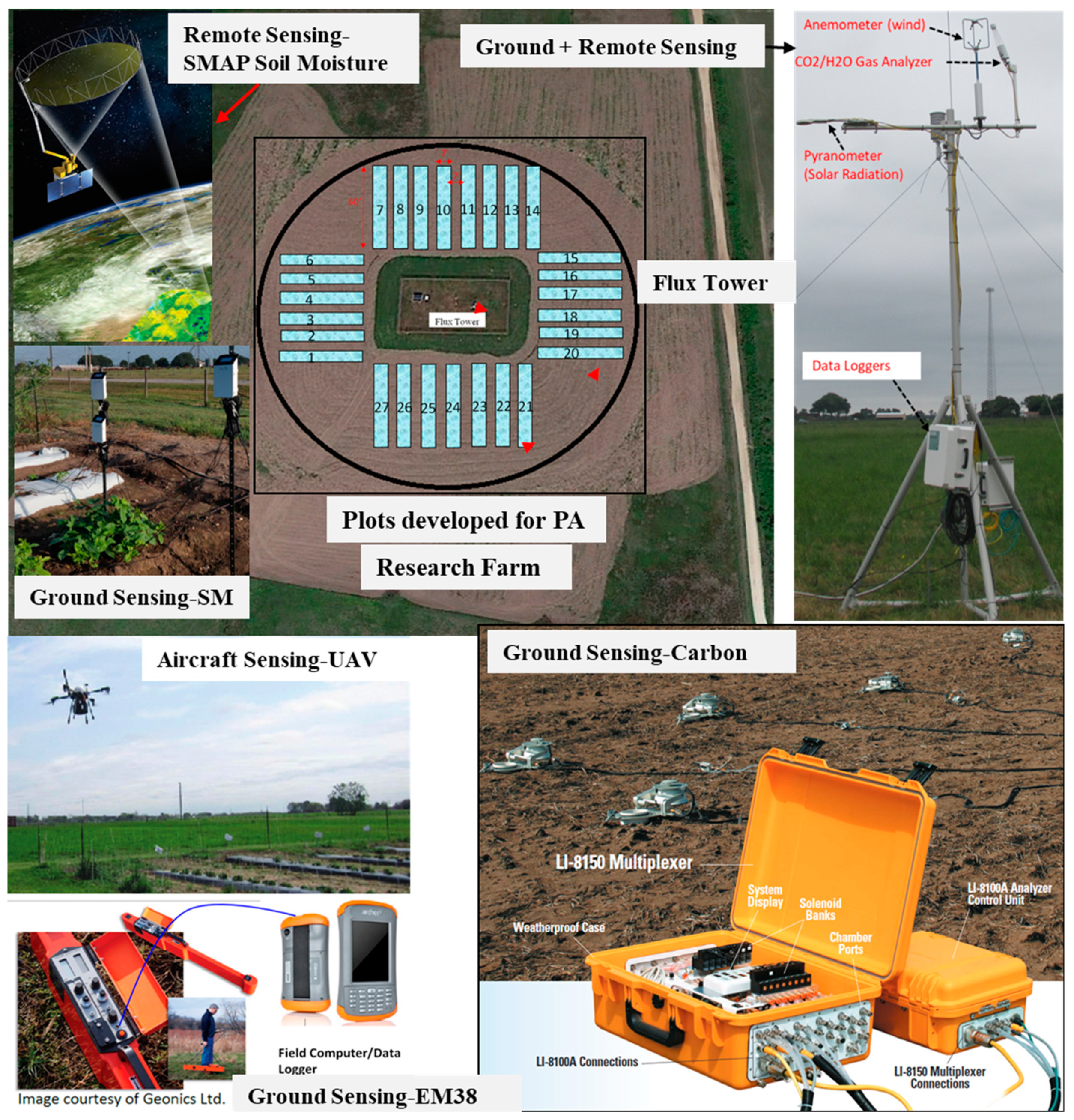
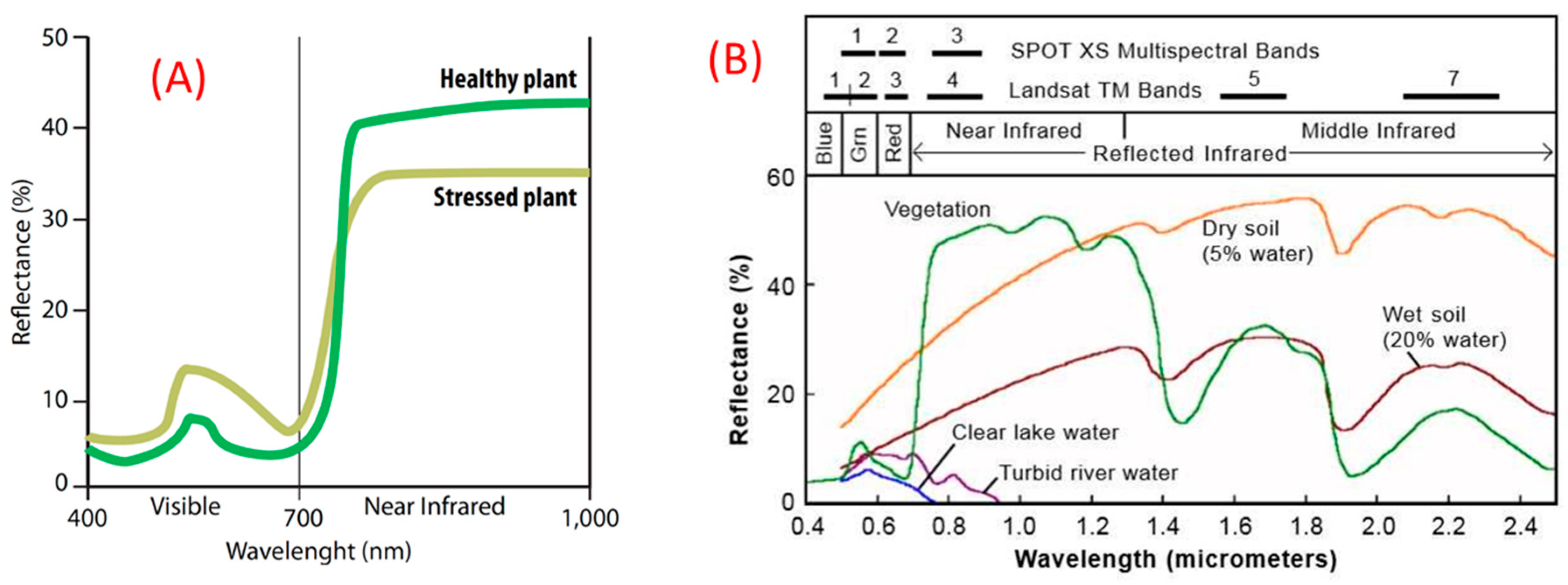
Table 1.
Spatiotemporal resolutions of the satellite sensors used for precision agricultural (PA) applications. Satellites that provide high spatial (<30 m) and temporal resolutions (e.g., daily) are more suitable for PA.
Table 1.
Spatiotemporal resolutions of the satellite sensors used for precision agricultural (PA) applications. Satellites that provide high spatial (<30 m) and temporal resolutions (e.g., daily) are more suitable for PA.
| Satellite (Years Active) | Sensor (Spatial Resolution) | Temporal Resolution | Application in Precision Agriculture |
|---|---|---|---|
| Landsat 1 (1972–1978) | MS (80 m) | 18 days | Crop growth [76] |
| AVHRR (1979-present) | MS (1.1 km) | 1 day | Nutrient management [77] |
| Landsat 5 TM (1984–2013) Landsat 7 (1999-present) Landsat 8 (2013-present) | MS and Thermal (60 m–Landsat 7, 100 m–Landsat 8, 120 m–Landsat 5) | 16 days | Biomass [78]; crop yield [79]; crop growth [80] |
| SPOT 1 (1986–1990) SPOT-2 (1990–2009) | MS (20 m) | 2–6 days | Water management [81] |
| IRS 1A (1988–1996) | MS (72 m) | 22 days | Water management, nutrient management [82] |
| LiDAR (1995) | VIS (10 cm) | N/A | Topography, nutrient management [83] |
| RadarSAT (1995–2013) | C-band SAR (30 m) | 1–6 days | Crop growth [84] |
| IKONOS (1999–2015) | MS (3.2 m) | 3 days | Crop yield [85]; soil properties [86]; nutrient management [77]; ET estimation [87] |
| EO-1 Hyperion (2000–2017) | HS (30 m) | 16 days | Disease [88,89] |
| Terra/Aqua MODIS (Terra-1999-present, Aqua-2002-present) | MS (SpectroRadiometer; 250–1000 m) | 1–2 days | Crop yield [90]; crop growth [91] |
| Terra-ASTER (2000-present) | MS and Thermal (15 m–V, NIR, 30 m–SWIR, 90 m–TIR) | 16 days | Water management [92] |
| QuickBird (2001–2014) | MS (2.44 m) | 1–3.5 days | Disease [93] |
| AQUA AMSR-E (2002–2016) | MS (Microwave Radiometer; 5.4 km–56 km) | 1–2 days | Water management [94] |
| Spot-5 (2002–2015) | MS (V, NIR–10 m, SWIR–20 m) | 2–3 days | Crop yield [95] |
| ResourceSat-1 (2003–2013) | MS (5.6m–V, 23.5 m–SWIR) | 5 days | Nutrient management [96] |
| KOMPSAT-2 (2006-present) | MS (4 m) | 5.5 days | Crop yield [97] |
| Radarsat-2 | C-band SAR (1–100 m) | 3 days | LAI and biomass [98] |
| RapidEye (2008-present) | MS (6.5 m) | 1–5.5 days | Water management [99]; crop yield [100]; crop growth and chlorophyll [101] |
| GeoEye-1 (2008-present) | MS (1.65 m) | 2.1–8.3 days | Nutrient management [102] |
| WorldView-2 (2009-present) | MS (1.4 m) | 1.1 days | Crop growth [103] |
| Pleiades-1A (2011-present) Pleiades-1B (2012-present) | MS (2 m) | 1 day | Crop growth [104,105] |
| VIIRS Suomi-NPP (2011-present) VIIRS-JPSS-1 (2017-present) | MS (IR Radiometer, 375 m and 750 m) | 16 day (repeat) | Crop management (NDVI [106]) |
| KOMPSAT-3 (2012-present) | MS (2.8 m) | 1.4 days | Crop growth [107] |
| Spot-6 (2012-present), Spot-7 (2014-present) | MS (6 m) | 1-day | Disease [108] |
| SkySat-1 (2013-present) SkySat-2 (2014-present) | MS (1 m) | sub-daily | Crop growth [109] |
| Worldview-3 (2014-present) | SS (1.24 m) | <1 day | Crop growth [110]; weed management [102] |
| Sentinel-1 (2014-present) | C-band SAR (5–40 m) | 1–3 days | Crop growth |
| Sentinel-2 (2015-present) | MS (10 m–V and NIR, 20 m–Red edge and SWIR, 60 m–2 NIR) | 2–5 days | Yield [111]; N management [112] |
| KOMPSAT-3A (2015-present) | MS (V NIR–2.2 m, SWIR–5.5 m) | 1.4 days | Disease [113] |
| SMAP (2015-present) | L-band SAR (1–3 km) and radiometer (40 km) | 2–3 days | Crop yield [114]; water management [115] |
| TripleSat (2015-present) | MS (3.2 m) | 1 day | Crop growth [116] |
| ECOSTRESS-PHyTIR (2018-present) | Thermal (38 × 69 m) | 1–5 days | ET [117] |
Table 2.
Some recently used vegetation indices for remote sensing applications in precision agriculture *.
Table 2.
Some recently used vegetation indices for remote sensing applications in precision agriculture *.
| Index | Definition/Equation | Applications (References) |
|---|---|---|
| Normalized difference vegetation index (NDVI) | Biomass [144]; breeding, phenotyping [145]; yield [146]; disease [108]; n-management [147]; soil moisture [148]; water stress [149] | |
| Green NDVI (GNDVI) | Water stress [150]; yield [151]; biomass [28,152,153]; disease [154] | |
| Normalized difference red edge (NDRE) | Crop yield and biomass [155]; N-management [147]; disease [154,156] | |
| Red edge normalized difference vegetation index (RENDVI) | Yield [100,111]; irrigation management [99]; N-status/application [140]; disease [156] | |
| Soil adjusted vegetation index (SAVI) | L-soil conditioning index | Yield [79]; biomass [28,153]; disease [157]; N-concentration and uptake [142]; water stress [158] |
| Modified soil adjusted vegetation index (MSAVI) | Biomass [153]; crop yield [159]; N-uptake [142]; chlorophyll content [112,160] | |
| Renormalized difference vegetation index (RDVI) | Crop yield [159]; N-uptake [142]; soil moisture [148]; biomass [28] | |
| Wide dynamic range vegetation index (WDRVI) | N-Application, yield [161]; crop growth (LAI) [162]; disease [113] | |
| Atmospherically resistant vegetation index (ARVI) | Disease [108]; weed mapping [163] | |
| Atmospherically effect resistant vegetation index (IAVI) | Crop yield [164] | |
| Ratio vegetation index (RVI) | Crop yield [159]; biomass [28] | |
| Difference vegetation index (DVI) | Disease [154]; crop yield [159]; LAI [142] | |
| Red edge DVI (REDVI) | Crop yield and biomass [155]; biomass, N-uptake, and concentration [142] | |
| Transformed soil adjusted vegetative index (TSAVI) | Water stress [158]; crop yield [165] | |
| Plant senescence reflectance index (PSRI) | Disease [166]; yield [167]; biomass [28] | |
| Normalized pigment chlorophyll ratio index (NPCI) | Water stress [168] | |
| Chlorophyll absorption ratio index (CARI) | Chlorophyll content [169] | |
| Modified chlorophyll and reflectance index (MCARI) | Crop growth–chlorophyll content [101] | |
| Chlorophyll vegetation index (CVI) | Crop yield [170]; crop growth-chlorophyll content [101]; yield [111] | |
| Chlorophyll index (CI) | Chlorophyll and N-content [171] | |
| Optimized soil adjusted vegetation index (OSAVI) | Disease [153]; crop yield [159]; biomass, N-uptake [28,142]; soil moisture [148]; water stress [158] | |
| Photochemical reflectance index (PRI) | Disease [172]; leaf water stress (PRInorm), canopy temperature and yield (PRI550) [148]; water stress (PRI, PRI550–515, PRInorm [149] | |
| Water balance index | Irrigation scheduling [173] | |
| Normalized difference water content (NDWI) | Vegetation water content [174] | |
| Shortwave infrared water stress index (SIWSI) | Leaf water content (water stress; [175]) | |
| Degrees above non-stressed canopy (DANS) | Water stress [176]; ET [177] | |
| Degrees above canopy threshold (DACT) | ET [177]; water stress [176] | |
| Triangular vegetation index (TVI) | Disease [108,156,172] | |
| Red-edge inflection point (REIP) | Yield and biomass [155] | |
| Enhanced vegetation index (EVI) | Disease [157]; biomass [28] | |
| Normalized water index (NWI) | Soil moisture and crop yield [148] |
* This list is an effort to compile some recently used vegetation indices, it is not meant to be a comprehensive list as there are many more indices that have been used in PA applications.
© 2020 by the authors. Licensee MDPI, Basel, Switzerland. This article is an open access article distributed under the terms and conditions of the Creative Commons Attribution (CC BY) license (http://creativecommons.org/licenses/by/4.0/).
Share and Cite
MDPI and ACS Style
Sishodia, R.P.; Ray, R.L.; Singh, S.K. Applications of Remote Sensing in Precision Agriculture: A Review. Remote Sens. 2020, 12, 3136. https://0-doi-org.brum.beds.ac.uk/10.3390/rs12193136
AMA Style
Sishodia RP, Ray RL, Singh SK. Applications of Remote Sensing in Precision Agriculture: A Review. Remote Sensing. 2020; 12(19):3136. https://0-doi-org.brum.beds.ac.uk/10.3390/rs12193136
Chicago/Turabian StyleSishodia, Rajendra P., Ram L. Ray, and Sudhir K. Singh. 2020. "Applications of Remote Sensing in Precision Agriculture: A Review" Remote Sensing 12, no. 19: 3136. https://0-doi-org.brum.beds.ac.uk/10.3390/rs12193136
Note that from the first issue of 2016, this journal uses article numbers instead of page numbers. See further details here.