Article

A High-Performance Spectral-Spatial Residual Network for Hyperspectral Image Classification with Small Training Data

1
Department of Computer Science and Software Engineering, The University of Western Australia, 35 Stirling Highway, Crawley, Perth, WA 6009, Australia
2
Department of Electrical, Electronic and Computer Engineering, The University of Western Australia, 35 Stirling Highway, Crawley, Perth, WA 6009, Australia
3
Information Technology, Mathematics & Statistics, Murdoch University, 90 South Street, Murdoch, Perth, WA 6150, Australia
4
School of Plant Biology and The UWA Institute of Agriculture, The University of Western Australia, 35 Stirling Highway, Crawley, Perth, WA 6009, Australia
*
Author to whom correspondence should be addressed.
Remote Sens. 2020, 12(19), 3137; https://0-doi-org.brum.beds.ac.uk/10.3390/rs12193137
Submission received: 13 August 2020 / Revised: 14 September 2020 / Accepted: 21 September 2020 / Published: 24 September 2020

Abstract

:
In this paper, we propose a high performance Two-Stream spectral-spatial Residual Network (TSRN) for hyperspectral image classification. The first spectral residual network (sRN) stream is used to extract spectral characteristics, and the second spatial residual network (saRN) stream is concurrently used to extract spatial features. The sRN uses 1D convolutional layers to fit the spectral data structure, while the saRN uses 2D convolutional layers to match the hyperspectral spatial data structure. Furthermore, each convolutional layer is preceded by a Batch Normalization (BN) layer that works as a regularizer to speed up the training process and to improve the accuracy. We conducted experiments on three well-known hyperspectral datasets, and we compare our results with five contemporary methods across various sizes of training samples. The experimental results show that the proposed architecture can be trained with small size datasets and outperforms the state-of-the-art methods in terms of the Overall Accuracy, Average Accuracy, Kappa Value, and training time.

Graphical Abstract

1. Introduction

Hyperspectral imaging has received much attention in recent years due to its ability to capture spectral information that is not detected by the naked human eye [1]. Hyperspectral imaging provides rich cues for numerous computer vision tasks [2] and a wide range of application areas, including medical [1], military [3], forestry [4], food processing [5], and agriculture [6].
One of the main challenges when analyzing Hyperspectral Images (HSIs) lies in extracting features, which is challenging due to the complex characteristics, i.e., the large size and the large spatial variability of HSIs [7]. Furthermore, HSI is composed of hundreds of spectral bands, in which wavelengths are very close, resulting in high redundancies [7,8]. Traditional machine learning methods are less suitable for HSI analysis because they heavily depend on hand-crafted features, which are commonly designed for a specific task, and are thus not generalizable [9]. In contrast, deep learning techniques can capture characteristic features automatically [9,10], thus constituting a promising avenue for HSI analysis.
Several deep learning architectures have been proposed to classify HSIs. Many architectures, such as one-dimensional convolutional neural network (1D-CNN) [11,12], one-dimensional generative adversarial network (1D-GAN) [13,14], and recurrent neural network (RNN) [15,16], have been proposed to learn spectral features. Other works, e.g., Reference [17,18,19], have shown that adding spatial features can improve the classification performance. Numerous spectral-spatial network architectures have been proposed for HSIs [19,20,21,22,23,24,25,26,27,28].
A number of methods argue that extracting the spectral and spatial features in two separate streams can produce more discriminative features [25,29,30]. Examples of such methods include stacked denoising autoencoder (SdAE) and 2D-CNN [30], plain 1D-CNN and 2D-CNN [25], spectral-spatial long short-term memory (SSLSTMs) [27], and a spectral-spatial unified network (SSUN) [23]. In terms of the spectral stream, the work of Reference [27] used a LSTM, which considers the spectral values of the different channels as a sequence. However, using LSTM on hundreds of a sequence of channels is complex; thus, [23] tried to simplify the sequence by grouping them. One of the grouping strategies is dividing the adjacent band into the same sequence following the spectral orders. The work in Reference [30] considered spectral values as a vector with noise and used a denoising technique, SdAE, to encode the spectral features. These networks, based on LSTM and SdAE, are all shallow. To increase the accuracy, Reference [25] tried to make a deeper network by employing a simpler layer, based on 1D convolution. The work in Reference [31] considered that the HSI bands have a different variance and correlation. Hence, they cluster the bands into some groups based on their similarity, then extracted the spectral features of each cluster using 1D convolution. Different from Reference [31], the study in Reference [32] considered that different objects have different spectral reflection profiles; hence, they used 2D convolution with a kernel size of 1x1 to extract the spectral features. For the spatial stream, Reference [27] also used LSTM, and due to its complexity, thus used a shallow network. Other approaches [23,25,30] used 2D convolution with a plain network, which could be made deeper, while Reference [31,32] used 2D convolution with a multi-scale input to extract multi-scale spatial features.
Other works claim that extracting spectral and spatial features directly using a single stream network can be more beneficial as it leverages the joint spectral-spatial features [28,33,34]. Most that adopt this approach utilize 3D convolutional layers [12,19,34,35] because they are naturally suited to the 3D cube data structure of HSIs. Reported experiments show that deep 3D-CNN produces better performance compared with 2D-CNN [18]. However, 3D-CNN requires large memory size and expensive computation cost [36]. Moreover, 3D-CNN faces over-smoothing phenomena because it fails to take the full advantage of spectral information, which results in misclassification for small objects and boundaries [23]. In addition, the labeling process of HSIs is labor-intensive, time-consuming, difficult, and thus expensive [37]. Using a complex deep learning architecture, in which parameters are in the millions, to learn from a small labeled dataset may also lead to over-fitting [38]. Moreover, adjusting millions of parameters during the deep-learning training process consumes a lot of time. Devising a deep learning architecture, which can work well on complex data of HSI, in which labeled datasets are small, is desirable.
Another issue with HSI classification based on deep learning is the depth of the network. The deeper the layer is, the richer the features will be, where the first layer of the deep network extracts general characteristics, and the deeper layers extract more specific features [39,40]. However, such deep networks are prone to the vanishing/exploding gradient problem, which occurs when the layers are deeper [41,42]. To solve this problem, Reference [40] reformulated the layers as learning residual functions with reference to the layer inputs. This approach is called a residual network (ResNet), which has become popular because of its remarkable performance on image classification [43]. For HSI classification, a single stream ResNet has been used by Reference [19,44,45,46].
Another problem related to HSI feature extraction is that the spectral values are prone to noise [47]. However, most of the previous research, which focus on the extraction of spectral features with deep-networks, have not taken noise into account. They usually use a pixel vector along the spectral dimension directly as their spectral network input [23,25,27,29,30], without considering that noise can worsen the classification performance.
Considering the aforementioned challenges and the limitations of existing network architectures, associated with HSI feature extraction and classification, we propose an efficient yet high performance two-stream spectral-spatial residual network. The spectral residual network (sRN) stream uses 1D convolutional layers to fit the spectral data structure, and the spatial residual network (saRN) uses 2D convolutional layers to fit the spatial data structure. The residual connection in the sRN and saRN can solve the vanishing/exploding gradient problem. Since proceeding the convolutional layer with Batch Normalization (BN) layer and full pre-activation rectified linear unit (ReLU) generalizes better than the original ResNet [48], in each of our residual unit, we use BN layer and ReLU layer before the convolutional layer. We then combine our sRN and saRN in a parallel pipeline. As shown in Figure 1, given a spectral input cube X i j s of a pixel x i j , the sRN extracts its spectral features. Concurrently, given a spatial input cube X i j s a of a pixel x i j , the saRN will extract its spatial characteristics. Since the sRN and the saRN use different input sizes and different types of convolution layers, they produce different sizes of feature maps. The gap between the number of spectral feature maps and the number of spatial feature maps can worsen the classification accuracy. To make the number of feature maps in each network proportional, we add an identical fully connected layer at the end of each network. Subsequently, we employ a dense layer to fuse the spectral features and the spatial features. Finally, we classify the joint spectral-spatial features using a softmax layer (Figure 1).
In summary, the main contributions of this research are:
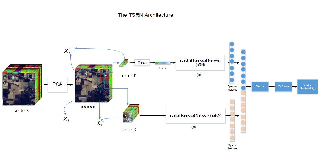
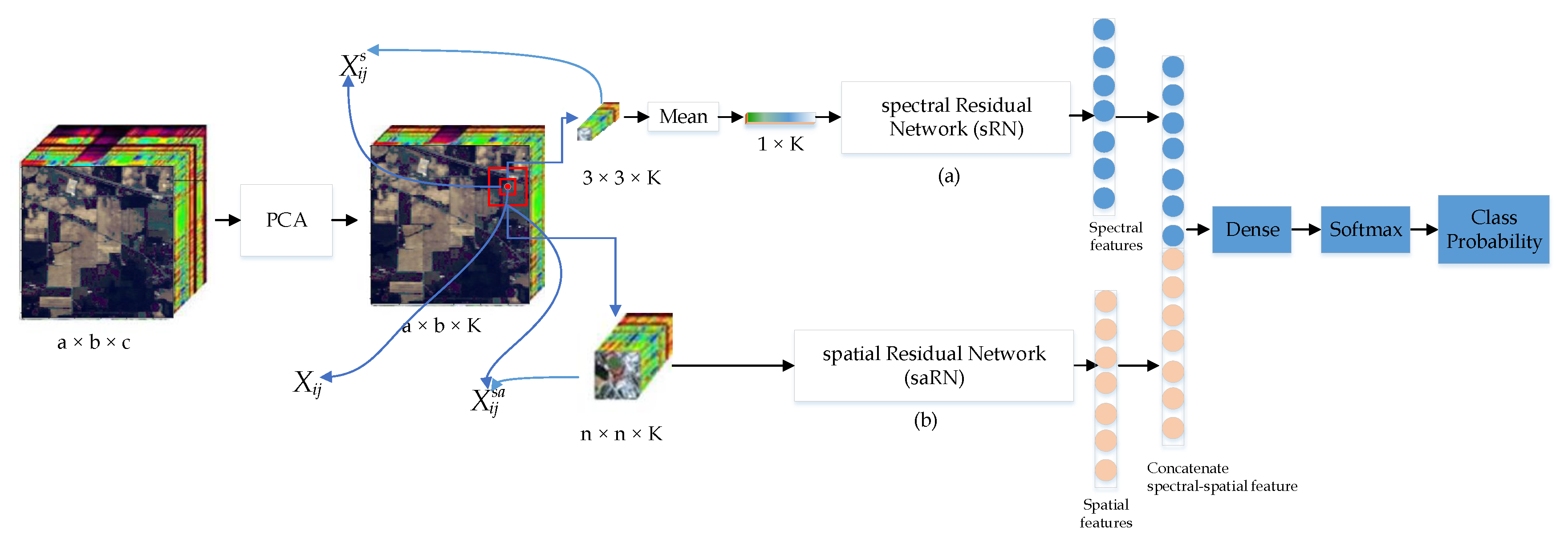
  • We propose TSRN, a Two-Stream Spectral-Spatial network with residual connections, to extract spectral and spatial features for HSI classification. The identity shortcut in the residual-unit is parameter-free, thus adding shortcut connections into a residual-unit does not increase the number of parameters. Furthermore, the use of 1D convolutional layers in the sRN and 2D convolutional layers in the saRN results in few trainable parameters. We can, therefore, construct a deeper and wider network with fewer parameters, making it particularly suitable for HSI classification when the amount of available labeled data is small.
  • We achieve the state-of-the-art performance on HSI classification with various sizes of training samples (4%, 6%, 8%, 10%, and 30%). Moreover, compared to networks based on 3D convolutional layers, our proposed architecture is faster.

2. Technical Preliminaries

2.1. CNN

Convolutional Neural Networks (CNNs) have been increasingly used for HSI analysis. A number of works aimed at improving the performance of Deep CNNs (DCNNs) have focused on different aspects, e.g., the network architecture, the type of nonlinear activation function, supervision methods, regularization mechanisms, and optimization techniques [4,49,50]. Based on the network architecture, specifically on the convolutional layers, there are different types of CNNs, namely 1D-CNN, 2D-CNN, and 3D-CNN. The 1D-CNN has one-dimensional filters in its convolutional layers which are naturally fit to the spectral data structure. Consider the case when the size of the input is K × 1 , and the kernel size is B × 1 , with K representing the number of HSI bands, B is the kernel size, and B < < K . Wei Hu et al. [11] used 1D convolutional layers to extract the spectral features of HSI. Their network input is an HSI pixel vector, with size ( K , 1 ) . This research initiated the use of multiple convolutional layers for HSI classification. Compared to 2D convolution and 3D convolution, the process of 1D convolution, which is shown in Equation (1), is the simplest one.
A 2D-CNN has two-dimensional filters in its convolutional layers. It has been widely used to solve several computer vision problems, such as object detection [51], scene recognition [52], and image classification [51], because of its ability to extract features from a raw image directly. For the HSI classification problem, 2D convolutions have been used to extract spatial features [25,30]. In contrast to RGB images, HSI has a much larger number of channels. Applying 2D convolutions along the hundreds of channels results in more learned parameters [18]; hence, several studies on HSIs, which employ 2D convolutions, do not use all of the channels. Most of them use a dimensionality reduction technique as a preprocessing step with their network [53,54,55] or use the average of all the images over the spectral bands of the HSI [25].
A 3D-CNN employs 3D convolutions in its convolutional layers. 3D-CNNs are popular for video classification [36], 3D object reconstruction [56], and action recognition [57]. For the case of HSIs, the form of the 3D filter suits the data structure of the HSI cube. Some research papers on HSI classification use 3D convolutional layers to extract the spectral-spatial features directly [18,33]. Their research shows that 3D-CNN outperforms both 1D-CNN and 2D-CNN. However, as shown in Equation (3), the process of 3D convolution requires more parameters, more memory, and requires a higher computational time and complexity compared to 1D convolution in Equation (1) and 2D convolution in Equation (2).
v i j z = f ( m b = 0 B i 1 k i j m b v ( i 1 ) m z + b + r i j ) ,
v i j x y = f ( m h = 0 H i 1 w = 0 W i 1 k i j m w h v ( i 1 ) m ( x + h ) ( y + w ) + r i j ) ,
v i j x y z = f ( m b = 0 B i 1 h = 0 H i 1 w = 0 W i 1 k i j m w h b v ( i 1 ) m ( x + h ) ( y + w ) ( z + b ) + r i j ) ,
where: i is the layer under consideration, m is the index of feature map, z is the index that corresponds to the spectral dimension, v i j z is the output of the i th layer and the j th feature map at position z, k i j m b is the kernel value at index b on the layer i and feature map j, r i j is the bias at layer i and feature map j. For the 1D convolution in Equation (1), B i is the size of the 1D filter in layer i, while, for the 3D convolution in Equation (3), B i is the depth of 3D kernel. W i and H i are the width and height of the kernel, respectively, for both 2D and 3D convolutions.
The expensive computational cost and memory demand of 3D convolution has led studies to investigate alternative network architectures based on (2D + 1D) convolutions. For instance, in the case of action recognition, a study in Reference [58] proposed to replace 3D convolution with m parallel streams of n 2D and one 1D convolution. This study empirically showed that their network, which is based on (2D + 1D) convolution, achieves around 40% reduction in model size and yields a drastic reduction in the number of learning parameters compared to another network with 3D convolution. In Reference [36], a simplified 3D convolution was implemented using 2D and 1D convolutions in three different blocks: 2D followed by 1D, 2D and 1D in parallel, and 2D followed by 1D with skip connections. These blocks were subsequently interleaved using a sequence network. The proposed architecture has a depth of 199 and a model size of 261 MB, which is much lighter compared to the 3D-CNN, in which model size is 321 MB when the depth is 11. The architecture was also shown to be faster than its 3D-CNN counterpart [36]. Using (2D + 1D) convolutions instead of 3D convolutions allows the network to be deeper without significantly increasing the number of parameters. Such deep networks can extract richer features and have been shown to outperform 3D-CNN architectures [36,58,59]. Because the model size and the number of parameters grow dramatically as the network becomes deeper, the training of deep 3D-CNNs is extremely difficult with the risk of overfitting.

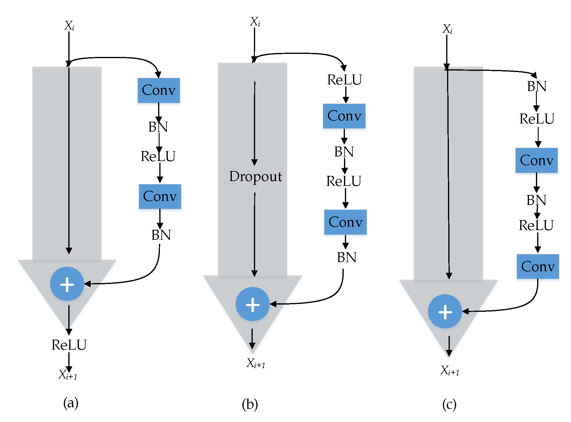
2.2. Residual Network

Deeper CNN can extract richer features [39]. In some cases, when the networks are deeper, their accuracy degrades because of the vanishing/exploding gradients problem [60]. Hence, He et al. [40] proposed to use a shortcut connection to perform identity mapping without adding extra parameters or extra computational time. The shortcut connection outputs are added to the output of the stacked layers, and a ReLU is applied as the activation function. This network is named ResNet. It has achieved outstanding classification accuracy on some image benchmark datasets, such as ImageNet, ILSVRC 2015, and CIFAR-10.
He et al. [48] followed up their work on ResNet by analyzing the propagation formulation behind the residual unit. Their analysis has shown that a “clean” information path in the skip connection results in the lowest training loss compared to those with scaling, gating, and convolution. Regarding the position of the ReLU activation function in the residual building blocks, they proved that putting ReLU and BN before the add function (full pre-activation) generalizes better than the original ResNet [40], which used ReLU after the add function (post-activation). The difference between pre-activation and post-activation in the residual building blocks is shown in Figure 3.
For the use of ResNet for HSI classification, Zhong et al. [44] proved that with the same size of convolutional layers, ResNet achieves better recognition accuracy than a plain CNN. Then, they explored ResNet by applying more various kernel sizes to sequentially extract the spectral features and the spatial features [19]. Roy et al. [61] used 3D convolutional layers followed by 2D convolutional layers in their residual network. Their network achieved high performance with 30% training samples. Meanwhile, Reference [45] explored ResNet by implementing a variable number of kernels in each convolutional layer. The kernel number was set to increase gradually in all convolutional layers like a pyramid to increase the diversity of the spectral-spatial features. In contrast to Reference [19,45,61], which focus on exploring the convolutional layer, Reference [46] improved the ResNet architecture by combining it with a dense convolutional network, which helps the ResNet to explore new features. These various works all improve ResNet performance by using a single network to extract both spectral and spatial features. Our proposed architecture extracts the spectral and spatial features from two separate stream networks to produce distinctive spectral and spatial features.

3. Proposed TSRN Network

The flowchart of the proposed TSRN is displayed in Figure 1. From the diagram, we can see that TSRN has two important residual network streams: a sRN and a saRN. Since the number of bands in the spectral dimension is very large (hundreds of channels), and thus comprises much redundancy, we first apply PCA to extract the first K principal components. Then, for each pixel, we take a 3 × 3 cube alongside the spectral direction, which is centered at that pixel, as the input of the sRN stream to learn the spectral features. Similarly, we take an n × n × K cube and feed it to the saRN streams to extract the spatial features. In this method, we propose to use the same number of spectral and spatial features. Hence, we need to ensure that their feature map sizes at the output of the sRN and the saRN networks are the same. To this end, we have applied a dense layer with the same number of units in each stream. Then, we apply a fully connected layer to fuse the spectral features and the spatial features. Finally, we use a softmax layer to classify the features. In the next subsection, we will explain in more detail both spectral and spatial networks.

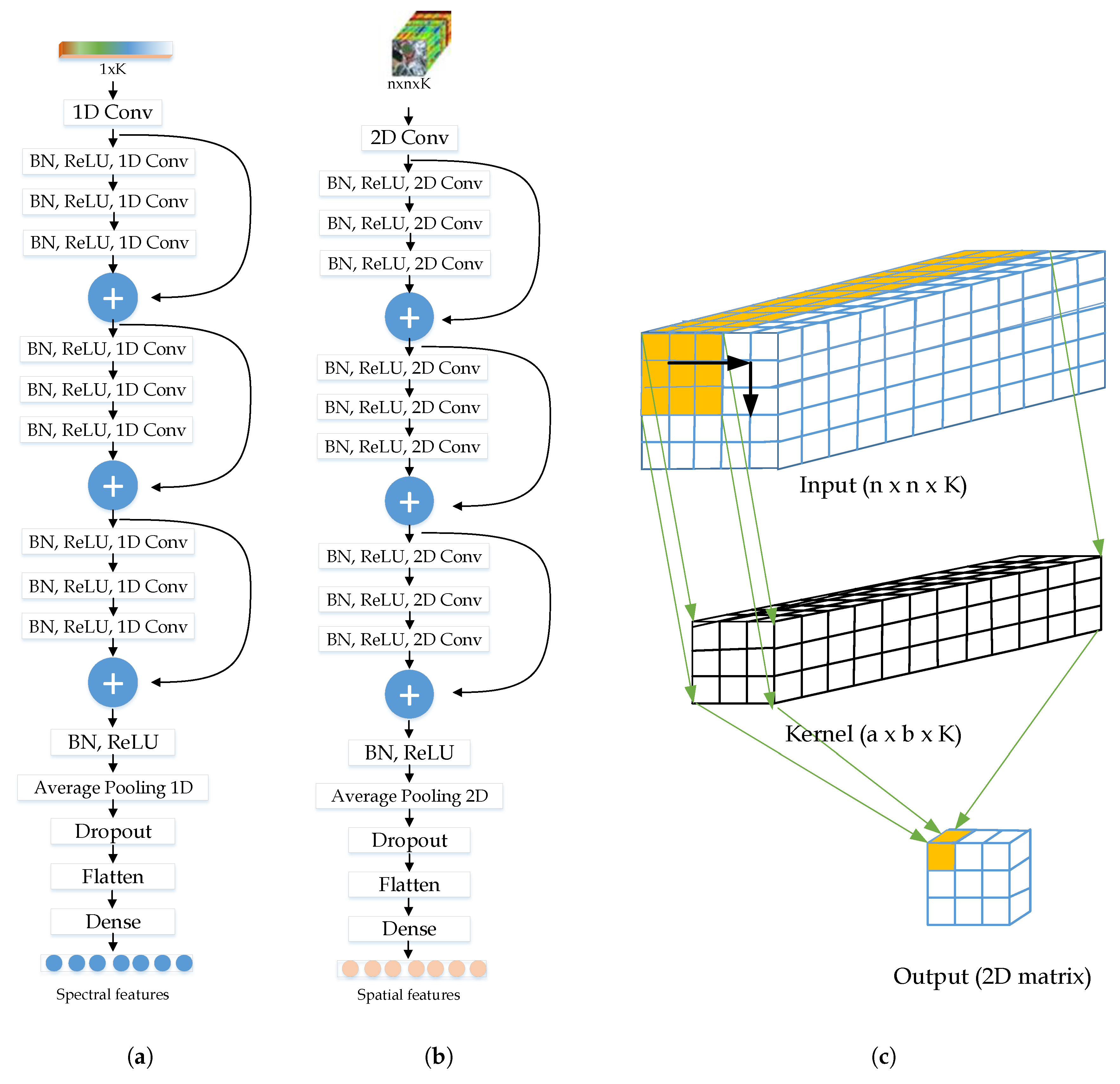
3.1. Spectral Residual Network

Although we have minimized the data redundancy of the HSI by using PCA, the spectral values can still be noisy. In the sRN, we propose to compute the mean of the reflectance in each spectral band before inputting the spectral cube into the sRN to minimize the effects of the noise. Given a pixel x i j , we choose a spectral cube X i j s R 3 × 3 × K , which is centered at x i j and K is the number of PCA components. Then, we compute the mean reflectance of each band by using Equation (4), where k K , X ¯ i j s = { x ¯ i j 1 s , x ¯ i j 2 s , . . . , x ¯ i j K s } , and X ¯ i j s R 1 x K .
x ¯ i j k s = h = j 1 h = j + 1 g = i 1 g = i + 1 x g , h , k s 9 .
Then, we input the mean of the spectral value ( X ¯ i j s ) into the sRN. In this proposed architecture, we use three full pre-activation with clear skip connection residual units inspired by Reference [48]. It has been shown that these residual units are better than the traditional residual units. These residual units consist of three different layers.
  • One-dimensional convolutional layers, which perform a dot product between every small window of input data ( 1 × B i ) and the kernel’s weights and biases (see Equation (1)).
  • BN layer that normalizes the layer inputs of each training mini-batch to overcome the internal covariate shift problem [62]. The internal covariate shift problem is a condition which occurs when the distribution of each layer’s inputs in deep-network changes due to the change of the previous layer’s parameters. This situation slows down the training. Normalizing the layer’s inputs stabilizes its distribution and thus speeds up the training process.
  • ReLU is an activation function, which learns the non-linear representations of each feature map’s components [63].
In the full pre-activation residual unit, the BN layer and the ReLU activation layer are established before the convolution layer, as shown in Figure 2a. From that figure, we can see that an Average Pooling layer, a Dropout layer, and a Dense layer have been applied at the end of the sRN. The Average Pooling layer and the Dropout layer are used as a regularizer to minimize the over-fitting problem due to the small number of training samples, while the Dense layer is used to perform the high-level reasoning to produce 128 spectral features.

3.2. Spatial Residual Network

The saRN is devised to extract the spatial features of a pixel x i j . The input is an n × n × K cube, centered at pixel x i j . Then, the input is processed by the full pre-activation residual unit. As shown in Figure 2b, the rest of the layers architecture of this saRN are similar to those of sRN. The main difference between them is that the saRN uses 2D convolutional layers, while the sRN uses 1D convolutional layers. In the end of this network, 128 spatial features are extracted.
Figure 2c illustrates the 2D convolution process with a spatial cube in which size is n × n × K , where K is the number of channels or the input depth. Since the input is 3D then the kernel is also 3D, i.e., the kernel depth must be the same as the input depth. Hence, in this case, the kernel depth must be K. So, we can only select the kernel width and height. The convolution process is performed along the x and y-direction and produces a 2D matrix as output [64].
Given a pixel x i j , the spectral features F i j s produced by sRN and the spatial features F i j s a produced by saRN are given by Equations (5) and (6), respectively.
F i j s = s R N ( X ¯ i j s ) ,
F i j s a = s a R N ( X i j s a ) .
Using F i j s and F i j s a , we implement a fully connected layer to obtain the joint spectral-spatial features F i j s s a using the formula in Equation (7), where W f c l and b f c l are the weight vector and the bias of the fully connected layer, respectively, and ⊕ is the concatenation operation.
F i j s s a = f ( W f c l · { F i j s F i j s a } + b f c l ) .
After obtaining the joint spectral-spatial feature F i j s s a , we use a softmax regression layer (SRL) to predict the class probability distribution of the pixel x i j by using Equation (8). Here, N is the number of classes, and P ( x i j ) is a vector consisting of the probability distribution of each class on pixel x i j . In the end, the label of the pixel x i j is decided using Equation (9).
P ( x i j ) = 1 n = 1 N e w n s r l . F i j s s a e w 1 s r l . F i j s s a e w 2 s r l . F i j s s a : e w N s r l . F i j s s a ,
l a b e l ( x i j ) = a r g m a x P ( x i j ) .

4. Experiments

4.1. Experimental Datasets

We evaluated the proposed architecture on three publicly available HSI datasets, which are frequently used for pixel-wise HSI classification. These datasets are Indian Pine (IP), Pavia University (PU), and Kennedy Space Center (KSC). These datasets were captured by different sensors, thus having different spatial resolutions and a different number of bands. Each dataset has a different category (class), and each class has a different number of instances. The details of the datasets are provided below:
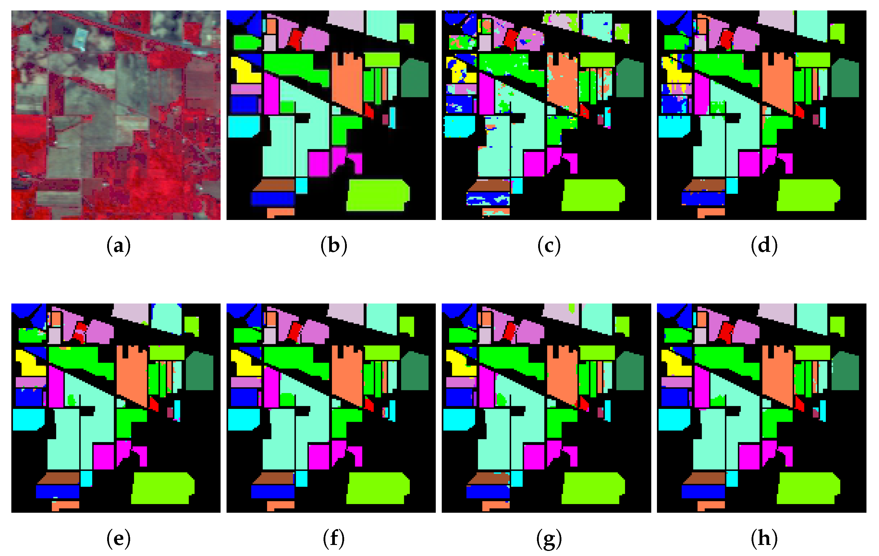
  • IP Dataset: IP dataset was acquired by Airborne Visible/Infrared Imaging Spectrometer (AVIRIS) hyperspectral sensor data on 12 June 1992, over Purdue University Agronomy farm and nearby area, in Northwestern Indiana, USA. The major portions of the area are Indian Creek and Pine Creek watershed; thus, the dataset is known as the Indian Pine dataset. The captured scene contains 145 × 145 pixels with a spatial resolution of 20 meters per pixel. In other words, the dataset has 21,025 pixels. However, not all of the pixels have ground-truth information. Only 10,249 pixels are categorized between 1 to 16 (as shown in Table 1a), and the remaining pixels remain unknown (labeled with zero in the ground truth). Regarding the spectral information, the entire spectral band of this dataset is 224, with wavelengths ranging from 400 to 2500 nm. Since some of the bands cover the region of water absorption, (104–108), (150–163), and 220, they are removed, so only 200 bands remain Reference [65].
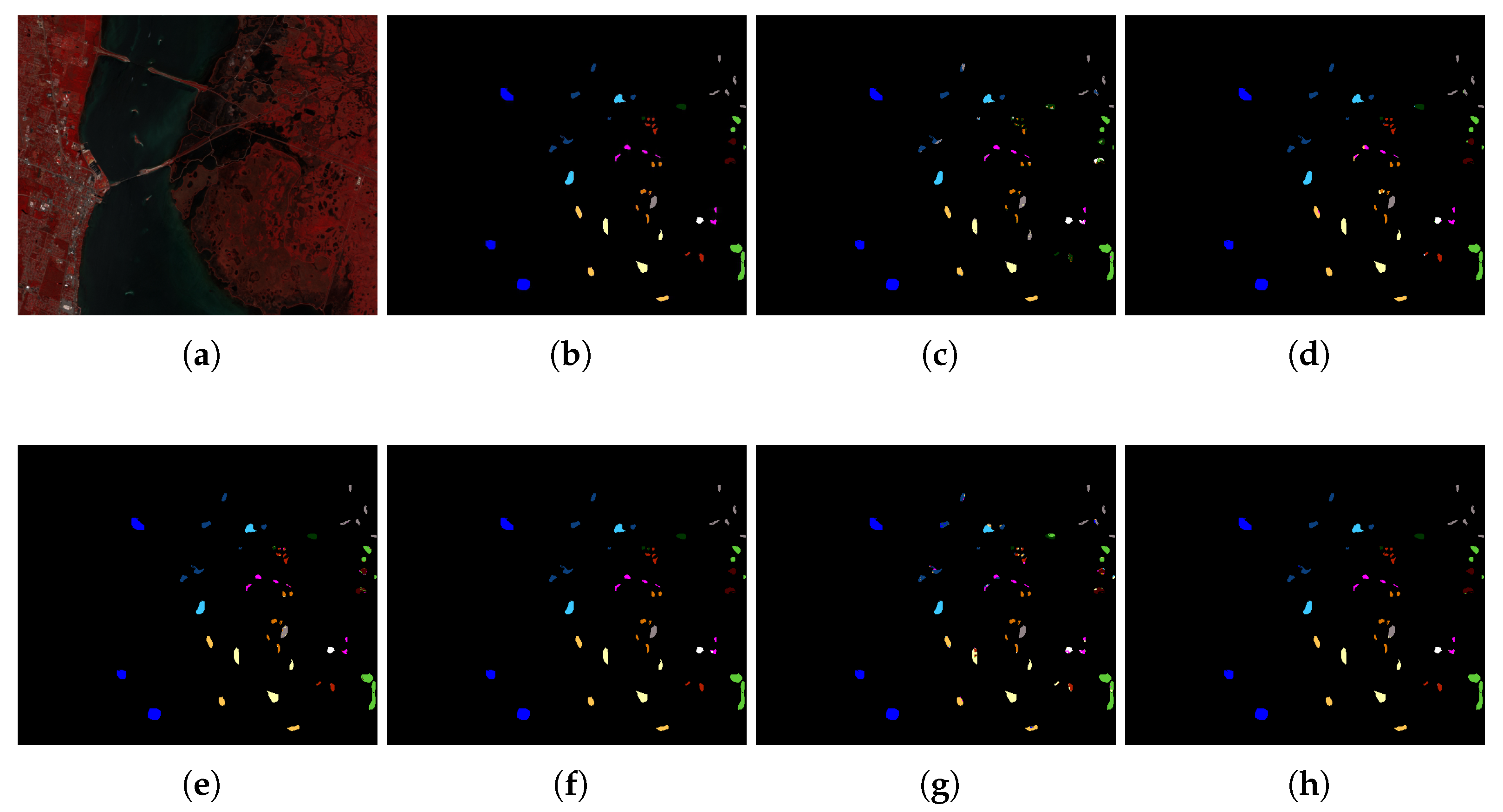
  • KSC Dataset: Same as the IP dataset, the KSC dataset was also collected by AVIRIS sensor in 1996 over the Kennedy Space Center, Florida, USA. Its size is 512 × 614 ; thus, this dataset consists of 314,368 pixels, but only 5122 pixels have ground-truth information (as shown in Table 1b). The dataset’s spatial resolution is 18 meters per pixel, and its band number is 174.
  • PU Dataset: The PU dataset was gathered during a flight campaign over the campus in Pavia, Northern Italy, using a Reflective Optics System Imaging Spectrometer (ROSIS) hyperspectral sensor. The dataset consists of 610 × 610 pixels, with a spatial resolution 1.3 meters per pixel. Hence 207,400 pixels are available in this dataset. However, only 20% of these pixels have ground-truth information, which are labeled into nine different classes, as shown in Table 1c. The number of its spectral bands is 103, ranging from 430 to 860 nm.

4.2. Experimental Configuration

In our proposed model, we do standardization (a technique to rescale the data to have a mean of 0 and a standard deviation of 1) in advance, before dividing the data into training and testing. Hyperparameters are initialized based on previous research or optimized during experiments. We initialized the convolution kernel by using the “He normal optimizer” [66] and applied l2 (0.0001) for the kernel regularizer. We use 1D convolutional kernels of size 5 in the sRN sub-network and 2D convolutional kernels of size 3 × 3 in the saRN sub-network. For the number of filters, we use the same size of filters in each convolution layer, 24. We apply 1D average pooling layer with pool size 2 and 2D average pooling layer with pool size 5 × 5 in the sRN and saRN, respectively. Furthermore, a 50% dropout is applied in both sub-networks. Then, we trained our model using Adam optimizer with a learning rate of 0.0003 [67].
Regarding batch-size, a constant batch-size sometimes results in a tiny mini-batch (see Figure 4a). Meanwhile, in a network with BN layers, there is dependency between the mini-batch elements because BN uses mini-batch statistics to normalize the activations during the learning process [68]. This dependency may decrease the performance if the mini-batch is too small [68,69]. Some approaches can be applied to overcome this problem. The first is to ignore the samples in the last mini-batch. This approach is not viable for the IP dataset because the number of training samples in a category can be very small; for example, with 10% training samples, we only have two training samples in Oats category. Performance will be badly affected if the removed samples are from this category (see Figure 4a). The second approach is by copying other samples from the previous mini-batch. This technique will make some samples appear twice in the training process, and these samples will have more weight. Another approach is by dividing the training size over the intended batch number. For example, if we intend to have three batches so the batch size = training size/3. However, when the training sample is too large, the batch size will be large and thus prone to an out of memory problem. If the training size is too small, the batch size will also be small, having a tiny batch size can decrease the performance. Therefore, in our experiment, we used Equation (10) to compute the batch-size prior to the training process to prevent the occurrence of a tiny mini-batch, where s b is the standard batch, t r is the training size, and t h is the threshold (the allowed smallest mini-batch, see Figure 4b). We used s b = 256 and t h = 64 in this paper.
b a t c h s i z e = s b , if t r mod s b > t h . s b + t r mod s b i n t ( t r s b ) , otherwise .
In the sRN, we used a 3 × 3 spectral cube and computed its mean instead of using a pixel vector directly to minimize the effect of spectral noise. In contrast to sRN, saRN focus is to get the spatial features; hence, the region size of the input cube gives an impact on the spatial feature representation. In this research, in order to find the optimum saRN input region size, n, we experiment on a variable set of n {21, 23, 25, and 27} with the number of PCA components set to 30 by using 10% random training samples and repeat the experiment 10 times. Table 2 shows the results of the Overall Accuracy mean and standard deviation, and from this table, we can conclude that each dataset has a different optimum number n. For the PU, IP, and KSC dataset, the optimum n is 21, 25, and 27, respectively.
We then use the optimum value of n to find the optimum number of PCA components, K. We experiment with different size of K {25, 30, 35, and 40}. The Overall Accuracy (OA)-mean with different values of K and 10% training samples are shown in Table 3. The table shows that the optimum K of KSC dataset is 25, while, for the IP dataset and PU dataset, the optimum K is 35.
Given the optimal parameters for our proposed method, we perform two experiments to understand the impact of each module of our proposed architecture. The first is an experiment to discover the effect of using the mean in the sRN sub-network. Second, we perform an experiment to evaluate the performance of sRN, saRN, and our proposed architecture.
To demonstrate the effectiveness of our proposed method, we compare our method with the state-of-the-art architectures, which focus on exploring the spectral-spatial features of HSI, namely 3D-CNN [34], SSLSTMs [27], SSUN [23], spectral-spatial residual network (SSRN) [19], and hybrid spectral convolutional neural network (HybridSN) [61]. The SSLSTMs and the SSUN explore the spectral and the spatial features using two different streams, while the 3D-CNN, the SSRN, and the HybridSN extract features using a single stream network based on 3D convolutional layer. The implementation codes of the 3D-CNN (https://github.com/nshaud/DeepHyperX), the SSUN (https://github.com/YonghaoXu/SSUN), the SSRN (https://github.com/zilongzhong/SSRN), and the HybridSN (https://github.com/gokriznastic/HybridSN) are publicly available, letting us execute the codes to produce the classification results with all datasets. For the SSLSTMs, even though the implementation code is not accessible, we wrote the code based on their paper architecture and parameters. To confirm that our implemented code is correct, we tested it on 10% of the training dataset and verified our results with the work of Reference [27]. All experiments except the 3D-CNN were conducted on X299 UD4 Pro desktop computer with the GeForce RTX 2080 Ti Graphical Processing Unit (GPU). The experiment of the 3D-CNN was conducted on Google Colab server because 3D-CNN used the Pytorch framework.
To validate the performance of the proposed model with respect to the training size of each compared model, we performed three different experiments. In all of these experiments, we used 10-fold cross-validation. To guarantee that all of the techniques use the same training indices and testing indices, we created a module to generate the training indices and testing indices by using StratifiedShuffleSplit function available in Keras. The input of this function is the training size percentage and the number of the fold/group (k). The output is k fold training indices and testing indices, where each fold is made by preserving the percentage of samples for each class. We then saved the training indices and testing indices of each fold in a file. Those files were read by each method during the experiment. Following the protocol in Reference [19], we use the same number of training epoch, 200, for all of the experiments. Regarding the hyperparameters, we used the optimum parameter of each model that has been provided in their respective paper. For the hyperparameters of this proposed approach, we used the optimum settings that have been optimized on 10% training samples, which were provided by Table 2 and Table 3.
In conclusion, we divided the experiments into two groups. The first group (experiments 1 and 2) is an ablation analysis to understand the impact of using the mean, and concatenating sRN and saRN in the proposed method with respect to the overall performance accuracy. The second group (experiments 3, 4, and 5) are experiments to understand the effectiveness of the proposed method compared to other previous studies. The details of these experiments are as follows:
  • To evaluate the effect of the mean operation in the sRN sub-network input, we performed experiments on our proposed architecture with two case scenarios. First, the sRN input is the mean of a 3 × 3 spectral cube. Second, the sRN input is a spectral vector of a pixel x i j without the mean operation. We performed experiments with 4%, 6%, 8%, 10%, and 30% training samples for IP dataset, PU dataset, and KSC dataset. We use the rest of the data that is not used in training for testing. In each run, we use the same data points for the training of both “with mean” and “without mean” setups.
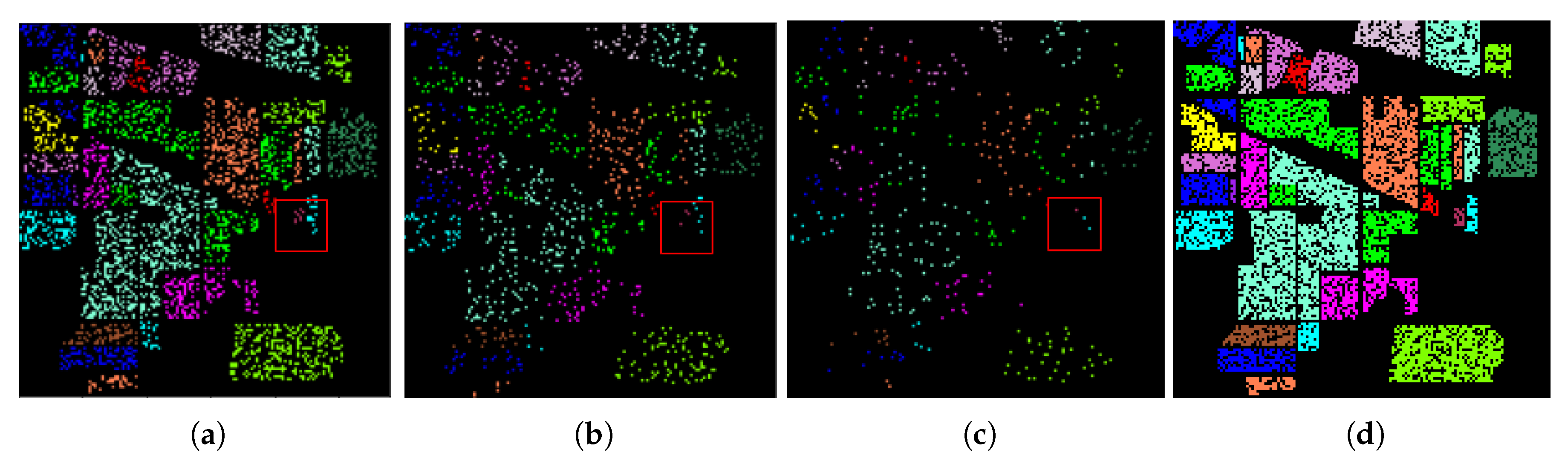
  • To discover the concatenation effect of the sRN sub-network and the saRN sub-network on the performance accuracy, we performed experiments on three different architectures, the sRN network only, the saRN network only, and our proposed method with 30%, 10%, and 4% training samples. Here, we divided the data into a training set (30%) and a testing set (70%). Then, from the training set, we used all, one-third, and one-seventh point five for training. For testing, in all experiments in this part, we used all data in the testing set. The examples of train and test split on IP dataset with various percentage training samples are shown in Figure 5.
  • In our third experiment, this proposed approach is compared to 3D-CNN, SSLSTMs, SSUN, SSRN, and HybridSN by using 10% training samples. We chose 10% training samples because the SSLSTMs and other experiments on SSUN, SSRN, and HybridSN have also been conducted using 10% training samples.
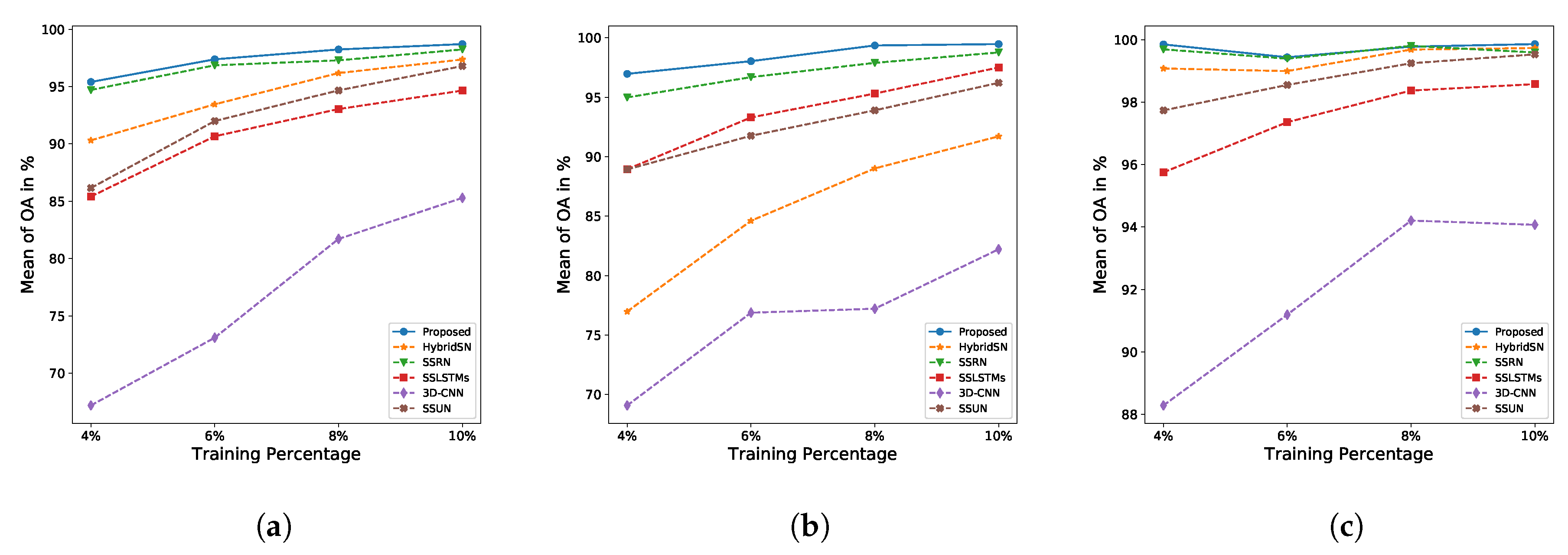
  • In our fourth experiment, we compared all of those methods on the smaller training samples, 4%, 6%, and 8%. Besides, because 3D-CNN has been tested using 4% training samples, the use of small labeled samples during training can be used to investigate over-fitting issues.
  • In the last experiment, we compared all of those methods on large training samples, 30%. Not only because HybridSN [61] had been tested on 30% training samples but also to investigate under-fitting issues with large training samples.

4.3. Experimental Results

Experiment 1: Table 4 shows the OA-mean and standard deviation of this proposed architecture in two different cases. In the first case, the sRN input of our network is a 3 × 3 cube followed by mean operations (with mean), and the second case, the sRN input of our network is a spectral vector, which was not followed by mean operations (without mean). From the table, we can see that, in 11 cases out of 15, the “with mean” slightly outperform the “without mean”. We also found that, in 10 cases out of 15, the “with mean” is more stable than “without mean”.
Experiment 2: Table 5 displays the OA-mean and standard deviation of sRN, saRN, and TSRN with various training samples, where the best performance is shown in bold. The table shows that with 30% training data, saRN’s performance is slightly better than others. With 10% training samples, TSRN’s performance starts to exceed saRN’s performance. TSRN’s superiority is clearly shown in 4% training samples. When the training size is large (30%), and the train and test sets are sampled randomly over the whole image, the possibility of the training samples become the testing samples’ neighbor is high. Other spatial features, such as line and shape, are clear, too. See Figure 5a, suppose the center of the red window is the testing sample, we can easily predict its label by seeing its spatial features. However, with 10% training samples, predicting the pixel’s label only by using its spatial features is slightly difficult (see Figure 5b). The prediction problems are more complicated when the training size is 4%. Figure 5c shows that the spatial features (e.g., neighborhood, shape, line) alone cannot perform well. Therefore, with 4% training samples, the TSRN, which also use spectral features, produces much better performance then saRN. Meanwhile, the low performance of sRN on IP dataset and KSC dataset probably because IP and KSC dataset have significantly low spatial resolution 20 m per pixel and 18 m per pixel, respectively. For example, in IP dataset, where most classes are vegetation, one pixel corresponds to the average reflectance of vegetation in 400 m 2 , which results in a mixture of ground materials. As a consequence, classifying the objects based on spectral information only is difficult.
Experiment 3: Table 6, Table 7 and Table 8 show the quantitative evaluations of those compared models with 10% training samples. The tables present three generally used quantitative metrics, i.e., Overall Accuracy (OA), Average Accuracy (AA), Kappa coefficient (K), and the classification accuracy of each class. The first three rows show the OA, AA, and K of each method. The following rows show the classification accuracy of each class. The numbers indicate the mean, followed by the standard deviation of each evaluation with a 10-fold cross-validation. The bold, the underlined, and the italic numbers represent the first-best performance, the second-best, and the third-best performance, respectively. Subsequently, Figure 6, Figure 7 and Figure 8 display the false-color image, the ground-truth image, and the classification map of each method on Indian Pine, Pavia University and KSC datasets.
Experiment 4: Figure 9 presents the graphic of AO-mean obtained from our fifth experiment, where all of those methods are trained on smaller training samples 4%, 6%, and 8%. In the figure, we include the results of our first experiment, where those methods are trained on the 10% samples. The performances of all of the compared methods are displayed using a dotted line, while our proposed method is displayed with a solid line.
Experiment 5: Table 9, Table 10 and Table 11 show the OA, AA, and K of each method with 30% training samples. On large training samples, almost all of the compared methods produce a high accuracy. The difference is small. Hence, in the table, we report the comparison on each fold for a more detailed comparison. The bold numbers are the best accuracies produced by these methods.

4.4. Discussion

According to the highlighted results in Section 4.3, one of the first apparent points is that the proposed method is able to produce a high performance for all ranges of training sizes (4%, 6%, 8%, 10%, and 30% training samples). Its OA, AA, and K values are higher compared to 3D-CNN, SSLSTMs, SSUN, SSRN, and HybridSN. The differences get higher as the training sample size is reduced. With large training samples, e.g., 30% training samples, the performances of these methods are similar.
The quantitative evaluation of those models with 10% training samples are reported in Table 6, Table 7 and Table 8. These tables show three standard quantitative metrics, i.e., OA, AA, K; and the classification accuracy of each class. More specifically, on Indian Pines dataset (see Table 6), in which class sizes are imbalanced, our proposed method produces the highest OA, AA, and K value, and the proposed approach yields OA 0.46% higher than the second-best method, SSRN. Considering the AA, the difference between the proposed architecture and SSRN is much higher, more than 7%. From Table 6, we can see that TSRN tries to optimize the recognition of each class even though the number of instances in the class is tiny. Hence, it achieves a high accuracy compared to the other methods when classifying C9 (Oats), in which number of instances is 20, which means C9 training samples is 2. For more detailed classification accuracy of each class, TSRN yields the best recognition on eight classes out of 16 classes. Its recognition for the other five classes and two classes are the second- and third-best, respectively.
The results are consistent on the Pavia University dataset, in which characteristics are different from the Indian Pine dataset. In the PU dataset, the number of data for each class is large, with the minimum number of instances on Shadows category equal to 947. As shown in Table 7, our proposed method attains the best OA, AA, and K compared to the other architectures, albeit insignificant disparity. The small gap between TSRN and the second-best method, HybridSN, shows that those methods are very competitive for large training samples. For class recognition, the proposed method achieves the highest accuracy on five out of nine classes in the PU dataset, with an improvement of less than 1%.
In contrast to the IP and PU datasets, the total number of instances of KSC dataset is relatively small. From Table 8, we can see that our proposed approach achieves the best performance. Its OA, AA, and K is ± 0.71, ± 0.94, and ± 0.79 higher compared to the second-best method, SSRN. In contrast, HybridSN yields performance that is not as good as its performance on IP and PU dataset.
The comparison between the proposed architecture and other methods on smaller training samples for IP, KSC, and PU dataset is demonstrated in Figure 9a–c, respectively. These figures reveal that the proposed method achieves the best accuracy even with smaller training samples. The accuracy gap between our method and the second-best method is high on KSC dataset. With 4% training data, our method achieves OA ± 2% higher than the second-best method, SSRN. The difference is smaller on IP dataset and is extremely small on PU dataset. The reason is that the size of the KSC dataset is the smallest compared to other datasets. Four percent training samples in the experiment correspond to 208 training instances on KSC dataset, 410 instances on IP dataset, and 1711 samples on PU dataset.
The performance of TSRN and the other methods with larger training samples, 30%, is shown in Table 9, Table 10 and Table 11 for IP dataset, PU dataset, and KSC dataset, respectively. In IP dataset, out of ten folds, the proposed method achieves the best OA and K on five-folds, and the best AA on eight folds. Our method also outperforms HybridSN, which presents the best OA on three folds. In PU dataset (see Table 10), the HybridSN shows a slightly better OA than the proposed architecture. HybridSN produces the best OA on six-folds while TSRN produces the best performance within five-folds. In the 2nd fold and 5th fold, their OA is precisely the same. Regarding AA, the proposed method achieves the best AA on six-folds when HybridSN achieves the best AA on four-folds. In terms of K, those two methods yield the best value on five-folds. The same with the result from IP dataset, with KSC dataset, our proposed approach also produces the best performance or the second-best performance in each fold (see Table 11). From these results, we can conclude that on large training samples, those approaches, i.e., TSRN, SSUN, HybridSN, SSRN, SSLSTMs, are very competitive.
Table 12 presents the number of parameters, the model size, the depth, the training time, and the testing time of the other methods with 10% training samples from IP dataset. We do not report the time complexity of 3D-CNN because 3D-CNN was tested on a different machine. However, Reference [61] has shown that 3D-CNN is less efficient compared to HybridSN. Moreover, from Table 12, we perceive that the proposed method is more efficient than HybridSN. In other words, we can conclude that TSRN is much more efficient than 3D-CNN. Compared to 3D convolution-based SSRN [19] and (3D + 2D) convolution-based HybridSN [61], our proposed network has a faster training time and fewer learning parameters (Table 12). Our network model size, in which depth is 24, is 3.3 MB. The size is smaller compared to 61.5 MB of a 7-layer HybridSN and more effective compared to 2.9 MB of a 9-layer SSRN. Note that an increase in the network depth results in a model size increase. From Table 12, we can see that our network, which uses (2D+1D) convolution, can be deeper without increasing the number of parameters by a large number. Such a deeper network can extract richer features. On the other hand, for 3D convolution, the model size and the number of parameters will grow dramatically as the network becomes deeper. As a result, training on very deep 3D-CNN becomes challenging with the risk of overfitting. Our network yields a smaller number of learnable parameters, making it less prone to the overfitting problem especially when small samples are used for training.

5. Conclusions

The paper presents a novel two-streams residual network architecture for the classification of hyperspectral data. Our network improves the spectral and the spatial feature extraction by applying a full pre-activation sRN and saRN separately. These two networks are similar in their structure but use a different type of convolutional layer. The convolutional layer of sRN is based on 1D convolution, which best fits the spectral data structure, while the saRN is based on 2D convolution, which best fits the spatial data structure of HSI.
Our experiments were conducted on three well-known hyperspectral datasets, versus five different methods, as well as various sizes of training samples. One of the main conclusions that arises from our experiments is that our proposed method can provide a higher performance versus state-of-the-art classification methods, even with various training samples proportion from 4% training samples up to 30% training samples. The high accuracy of our proposed method on small training samples, 4%, shows that this method does not overfit. Otherwise, the competitive accuracy of our proposed method with large training samples, 30%, explains that this architecture is not under-fitting either.

Author Contributions

W.N.K. proposed the methodology, implemented it, did experiments and analysis, and wrote the original draft manuscript. M.B., F.B., and F.S. supervised the study, directly contributed to the problem formulation, experimental design and technical discussions, reviewed the writing, and gave insightful suggestions for the manuscript. D.E. supervised the study, reviewed the writing, gave insightful suggestions for the manuscript and provided resources. All authors have read and agreed to the published version of the manuscript.

Funding

W.N. Khotimah is supported by a scholarship from Indonesian Endowment Fund for Education, Ministry of Finance, Indonesia. This research is also supported by Australia Research Council Grants DP150100294, DP150104251, and Grains Research and Development Corporation Grant UWA2002-003RTX.

Conflicts of Interest

The authors declare no conflict of interest. The funders had no role in the design of the study; in the collection, analyses, or interpretation of data; in the writing of the manuscript, or in the decision to publish the results.

References

  1. Lu, G.; Fei, B. Medical hyperspectral imaging: A review. J. Biomed. Opt. 2014, 19, 010901. [Google Scholar] [CrossRef] [PubMed]
  2. Wang, L.; Sun, C.; Fu, Y.; Kim, M.H.; Huang, H. Hyperspectral Image Reconstruction Using a Deep Spatial-Spectral Prior. In Proceedings of the IEEE Conference on Computer Vision and Pattern Recognition (CVPR), Long Beach, CA, USA, 16–20 June 2019. [Google Scholar]
  3. Shimoni, M.; Haelterman, R.; Perneel, C. Hypersectral Imaging for Military and Security Applications: Combining Myriad Processing and Sensing Techniques. IEEE Geosci. Remote Sens. Mag. 2019, 7, 101–117. [Google Scholar] [CrossRef]
  4. Stuart, M.B.; McGonigle, A.J.S.; Willmott, J.R. Hyperspectral Imaging in Environmental Monitoring: A Review of Recent Developments and Technological Advances in Compact Field Deployable Systems. Sensors 2019, 19, 3071. [Google Scholar] [CrossRef] [PubMed] [Green Version]
  5. Ma, J.; Sun, D.W.; Pu, H.; Cheng, J.H.; Wei, Q. Advanced Techniques for Hyperspectral Imaging in the Food Industry: Principles and Recent Applications. Annu. Rev. Food Sci. Technol. 2019, 10, 197–220. [Google Scholar] [CrossRef] [PubMed]
  6. Mahlein, A.K.; Kuska, M.; Behmann, J.; Polder, G.; Walter, A. Hyperspectral Sensors and Imaging Technologies in Phytopathology: State of the Art. Annu. Rev. Phytopathol. 2018, 56, 535–558. [Google Scholar] [CrossRef] [PubMed]
  7. Li, S.; Wu, H.; Wan, D.; Zhu, J. An effective feature selection method for hyperspectral image classification based on genetic algorithm and support vector machine. Knowl. Based Syst. 2011, 24, 40–48. [Google Scholar] [CrossRef]
  8. Cao, F.; Yang, Z.; Ren, J.; Ling, W.K.; Zhao, H.; Sun, M.; Benediktsson, J.A. Sparse representation-based augmented multinomial logistic extreme learning machine with weighted composite features for spectral–spatial classification of hyperspectral images. IEEE Trans. Geosci. Remote Sens. 2018, 56, 6263–6279. [Google Scholar] [CrossRef] [Green Version]
  9. Li, S.; Song, W.; Fang, L.; Chen, Y.; Ghamisi, P.; Benediktsson, J.A. Deep Learning for Hyperspectral Image Classification: An Overview. IEEE Trans. Geosci. Remote Sens. 2019, 57, 6690–6709. [Google Scholar] [CrossRef] [Green Version]
  10. Shah, S.A.A.; Bennamoun, M.; Boussaïd, F. Iterative deep learning for image set based face and object recognition. Neurocomputing 2016, 174, 866–874. [Google Scholar] [CrossRef]
  11. Hu, W.; Huang, Y.; Wei, L.; Zhang, F.; Li, H. Deep Convolutional Neural Networks for Hyperspectral Image Classification. J. Sens. 2015, 2015, 1–12. [Google Scholar] [CrossRef] [Green Version]
  12. Haut, J.M.; Paoletti, M.E.; Plaza, J.; Li, J.; Plaza, A. Active learning with convolutional neural networks for hyperspectral image classification using a new bayesian approach. IEEE Trans. Geosci. Remote Sens. 2018, 56, 6440–6461. [Google Scholar] [CrossRef]
  13. Zhu, L.; Chen, Y.; Ghamisi, P.; Benediktsson, J.A. Generative Adversarial Networks for Hyperspectral Image Classification. IEEE Trans. Geosci. Remote Sens. 2018, 56, 5046–5063. [Google Scholar] [CrossRef]
  14. Zhan, Y.; Hu, D.; Wang, Y.; Yu, X. Semisupervised Hyperspectral Image Classification Based on Generative Adversarial Networks. IEEE Geosci. Remote Sens. Lett. 2018, 15, 212–216. [Google Scholar] [CrossRef]
  15. Angelopoulou, T.; Tziolas, N.; Balafoutis, A.; Zalidis, G.; Bochtis, D. Remote Sensing Techniques for Soil Organic Carbon Estimation: A Review. Remote Sens. 2019, 11, 676. [Google Scholar] [CrossRef] [Green Version]
  16. Yang, X.; Ye, Y.; Li, X.; Lau, R.Y.; Zhang, X.; Huang, X. Hyperspectral image classification with deep learning models. IEEE Trans. Geosci. Remote Sens. 2018, 56, 5408–5423. [Google Scholar] [CrossRef]
  17. Liu, B.; Gao, G.; Gu, Y. Unsupervised Multitemporal Domain Adaptation With Source Labels Learning. IEEE Geosci. Remote Sens. Lett. 2019, 16, 1477–1481. [Google Scholar] [CrossRef]
  18. Li, Y.; Zhang, H.; Shen, Q. Spectral–Spatial Classification of Hyperspectral Imagery with 3D Convolutional Neural Network. Remote Sens. 2017, 9, 67. [Google Scholar] [CrossRef] [Green Version]
  19. Zhong, Z.; Li, J.; Luo, Z.; Chapman, M. Spectral–Spatial Residual Network for Hyperspectral Image Classification: A 3-D Deep Learning Framework. IEEE Trans. Geosci. Remote Sens. 2018, 56, 847–858. [Google Scholar] [CrossRef]
  20. Wang, W.; Dou, S.; Jiang, Z.; Sun, L. A Fast Dense Spectral–Spatial Convolution Network Framework for Hyperspectral Images Classification. Remote Sens. 2018, 10, 1068. [Google Scholar] [CrossRef] [Green Version]
  21. PV, A.; Buddhiraju, K.M.; Porwal, A. Capsulenet-Based Spatial–Spectral Classifier for Hyperspectral Images. IEEE J. Sel. Top. Appl. Earth Obs. Remote Sens. 2019, 12, 1849–1865. [Google Scholar] [CrossRef]
  22. Liu, Q.; Zhou, F.; Hang, R.; Yuan, X. Bidirectional-Convolutional LSTM Based Spectral-Spatial Feature Learning for Hyperspectral Image Classification. Remote Sens. 2017, 9, 1330. [Google Scholar] [CrossRef] [Green Version]
  23. Xu, Y.; Zhang, L.; Du, B.; Zhang, F. Spectral-Spatial Unified Networks for Hyperspectral Image Classification. IEEE Trans. Geosci. Remote Sens. 2018, 56, 5893–5909. [Google Scholar] [CrossRef]
  24. Koda, S.; Melgani, F.; Nishii, R. Unsupervised Spectral-Spatial Feature Extraction With Generalized Autoencoder for Hyperspectral Imagery. IEEE Geosci. Remote Sens. Lett. 2019, 17, 469–473. [Google Scholar] [CrossRef]
  25. Yang, J.; Zhao, Y.Q.; Chan, J.C.W. Learning and Transferring Deep Joint Spectral-Spatial Features for Hyperspectral Classification. IEEE Trans. Geosci. Remote Sens. 2017, 55, 4729–4742. [Google Scholar] [CrossRef]
  26. Hu, W.S.; Li, H.C.; Pan, L.; Li, W.; Tao, R.; Du, Q. Feature Extraction and Classification Based on Spatial-Spectral ConvLSTM Neural Network for Hyperspectral Images. arXiv 2019, arXiv:1905.03577. [Google Scholar]
  27. Zhou, F.; Hang, R.; Liu, Q.; Yuan, X. Hyperspectral image classification using spectral-spatial LSTMs. Neurocomputing 2019, 328, 39–47. [Google Scholar] [CrossRef]
  28. Liu, B.; Yu, X.; Zhang, P.; Tan, X.; Wang, R.; Zhi, L. Spectral–spatial classification of hyperspectral image using three-dimensional convolution network. J. Appl. Remote Sens. 2018, 12, 016005. [Google Scholar] [CrossRef]
  29. Pan, B.; Shi, Z.; Zhang, N.; Xie, S. Hyperspectral Image Classification Based on Nonlinear Spectral-Spatial Network. IEEE Geosci. Remote Sens. Lett. 2016, 13, 1782–1786. [Google Scholar] [CrossRef]
  30. Hao, S.; Wang, W.; Ye, Y.; Nie, T.; Bruzzone, L. Two-stream deep architecture for hyperspectral image classification. IEEE Trans. Geosci. Remote Sens. 2017, 56, 2349–2361. [Google Scholar] [CrossRef]
  31. Sun, G.; Zhang, X.; Jia, X.; Ren, J.; Zhang, A.; Yao, Y.; Zhao, H. Deep Fusion of Localized Spectral Features and Multi-scale Spatial Features for Effective Classification of Hyperspectral Images. Int. J. Appl. Earth Obs. Geoinf. 2020, 91, 102157. [Google Scholar] [CrossRef]
  32. Gao, L.; Gu, D.; Zhuang, L.; Ren, J.; Yang, D.; Zhang, B. Combining t-Distributed Stochastic Neighbor Embedding With Convolutional Neural Networks for Hyperspectral Image Classification. IEEE Geosci. Remote Sens. Lett. 2019, 17, 1368–1372. [Google Scholar] [CrossRef]
  33. He, M.; Li, B.; Chen, H. Multi-scale 3D deep convolutional neural network for hyperspectral image classification. In Proceedings of the 2017 IEEE International Conference on Image Processing (ICIP), Beijing, China, 17–20 September 2017; pp. 3904–3908. [Google Scholar] [CrossRef]
  34. Ben Hamida, A.; Benoit, A.; Lambert, P.; Ben Amar, C. 3-D deep learning approach for remote sensing image classification. IEEE Trans. Geosci. Remote Sens. 2018, 56, 4420–4434. [Google Scholar] [CrossRef] [Green Version]
  35. Paoletti, M.E.; Haut, J.M.; Fernandez-Beltran, R.; Plaza, J.; Plaza, A.; Li, J.; Pla, F. Capsule Networks for Hyperspectral Image Classification. IEEE Trans. Geosci. Remote Sens. 2019, 57, 2145–2160. [Google Scholar] [CrossRef]
  36. Qiu, Z.; Yao, T.; Mei, T. Learning spatio-temporal representation with pseudo-3d residual networks. In Proceedings of the IEEE International Conference on Computer Vision, Honolulu, HI, USA, 21–26 July 2017; pp. 5533–5541. [Google Scholar]
  37. Lin, J.; Zhao, L.; Li, S.; Ward, R.; Wang, Z.J. Active-Learning-Incorporated Deep Transfer Learning for Hyperspectral Image Classification. IEEE J. Sel. Top. Appl. Earth Obs. Remote Sens. 2018, 11, 4048–4062. [Google Scholar] [CrossRef]
  38. Alam, F.I.; Zhou, J.; Liew, A.W.C.; Jia, X.; Chanussot, J.; Gao, Y. Conditional Random Field and Deep Feature Learning for Hyperspectral Image Classification. IEEE Trans. Geosci. Remote Sens. 2019, 57, 1612–1628. [Google Scholar] [CrossRef] [Green Version]
  39. Zeiler, M.D.; Fergus, R. Visualizing and understanding convolutional networks. In Proceedings of the European Conference on Computer Vision, Zurich, Switzerland, 6–12 September 2014; pp. 818–833. [Google Scholar]
  40. He, K.; Zhang, X.; Ren, S.; Sun, J. Deep residual learning for image recognition. In Proceedings of the IEEE Conference on Computer Vision and Pattern Recognition, Las Vegas, NV, USA, 26 June 26–1 July 2016; pp. 770–778. [Google Scholar]
  41. Bengio, Y.; Simard, P.; Frasconi, P. Learning long-term dependencies with gradient descent is difficult. IEEE Trans. Neural Netw. 1994, 5, 157–166. [Google Scholar] [CrossRef] [PubMed]
  42. Glorot, X.; Bengio, Y. Understanding the difficulty of training deep feedforward neural networks. In Proceedings of the Thirteenth International Conference on Artificial Intelligence and Statistics, Sardinia, Italy, 13–15 May 2010; pp. 249–256. [Google Scholar]
  43. Hanif, M.S.; Bilal, M. Competitive residual neural network for image classification. ICT Express 2020, 6, 28–37. [Google Scholar] [CrossRef]
  44. Zhong, Z.; Li, J.; Ma, L.; Jiang, H.; Zhao, H. Deep residual networks for hyperspectral image classification. In Proceedings of the 2017 IEEE International Geoscience and Remote Sensing Symposium (IGARSS), Fort Worth, TX, USA, 23–28 July 2017; pp. 1824–1827. [Google Scholar]
  45. Paoletti, M.E.; Haut, J.M.; Fernandez-Beltran, R.; Plaza, J.; Plaza, A.J.; Pla, F. Deep pyramidal residual networks for spectral–spatial hyperspectral image classification. IEEE Trans. Geosci. Remote Sens. 2018, 57, 740–754. [Google Scholar] [CrossRef]
  46. Kang, X.; Zhuo, B.; Duan, P. Dual-path network-based hyperspectral image classification. IEEE Geosci. Remote Sens. Lett. 2018, 16, 447–451. [Google Scholar] [CrossRef]
  47. Aggarwal, H.K.; Majumdar, A. Hyperspectral Unmixing in the Presence of Mixed Noise Using Joint-Sparsity and Total Variation. IEEE J. Sel. Top. Appl. Earth Obs. Remote Sens. 2016, 9, 4257–4266. [Google Scholar] [CrossRef]
  48. He, K.; Zhang, X.; Ren, S.; Sun, J. Identity mappings in deep residual networks. In Proceedings of the European Conference on Computer Vision, Amsterdam, The Netherlands, 8–16 October 2016; pp. 630–645. [Google Scholar]
  49. Rawat, W.; Wang, Z. Deep convolutional neural networks for image classification: A comprehensive review. Neural Comput. 2017, 29, 2352–2449. [Google Scholar] [CrossRef]
  50. Khan, S.H.; Rahmani, H.; Shah, S.A.A.; Bennamoun, M. A Guide to Convolutional Neural Networks for Computer Vision; Morgan & Claypool: San Rafael, CA, USA, 2018. [Google Scholar]
  51. Kim, J.; Song, J.; Lee, J.K. Recognizing and Classifying Unknown Object in BIM Using 2D CNN. In Proceedings of the International Conference on Computer-Aided Architectural Design Futures, Daejeon, Korea, 26–28 June 2019; pp. 47–57. [Google Scholar]
  52. Parmar, P.; Morris, B. HalluciNet-ing Spatiotemporal Representations Using 2D-CNN. arXiv 2019, arXiv:1912.04430. [Google Scholar]
  53. Chen, Y.; Zhu, L.; Ghamisi, P.; Jia, X.; Li, G.; Tang, L. Hyperspectral Images Classification with Gabor Filtering and Convolutional Neural Network. IEEE Geosci. Remote Sens. Lett. 2017, 14, 2355–2359. [Google Scholar] [CrossRef]
  54. He, N.; Paoletti, M.E.; Haut, J.M.; Fang, L.; Li, S.; Plaza, A.; Plaza, J. Feature extraction with multiscale covariance maps for hyperspectral image classification. IEEE Trans. Geosci. Remote Sens. 2019, 57, 755–769. [Google Scholar] [CrossRef]
  55. Fang, L.; Liu, G.; Li, S.; Ghamisi, P.; Benediktsson, J.A. Hyperspectral Image Classification With Squeeze Multibias Network. IEEE Trans. Geosci. Remote Sens. 2019, 57, 1291–1301. [Google Scholar] [CrossRef]
  56. Han, X.F.; Laga, H.; Bennamoun, M. Image-based 3D Object Reconstruction: State-of-the-Art and Trends in the Deep Learning Era. IEEE Trans. Pattern Anal. Mach. Intell. 2019. [Google Scholar] [CrossRef] [Green Version]
  57. Hara, K.; Kataoka, H.; Satoh, Y. Can spatiotemporal 3d cnns retrace the history of 2d cnns and imagenet? In Proceedings of the IEEE Conference on Computer Vision and Pattern Recognition, Salt Lake City, UT, USA, 18–22 June 2018; pp. 6546–6555. [Google Scholar]
  58. Gonda, F.; Wei, D.; Parag, T.; Pfister, H. Parallel separable 3D convolution for video and volumetric data understanding. arXiv 2018, arXiv:1809.04096. [Google Scholar]
  59. Tran, D.; Wang, H.; Torresani, L.; Ray, J.; LeCun, Y.; Paluri, M. A closer look at spatiotemporal convolutions for action recognition. In Proceedings of the IEEE Conference on Computer Vision and Pattern Recognition, Salt Lake City, UT, USA, 18–22 June 2018; pp. 6450–6459. [Google Scholar]
  60. He, K.; Sun, J. Convolutional neural networks at constrained time cost. In Proceedings of the IEEE Conference on Computer Vision and Pattern Recognition, Boston, MA, USA, 7–12 June 2015; pp. 5353–5360. [Google Scholar]
  61. Roy, S.K.; Krishna, G.; Dubey, S.R.; Chaudhuri, B.B. Hybridsn: Exploring 3-d-2-d cnn feature hierarchy for hyperspectral image classification. IEEE Geosci. Remote Sens. Lett. 2019, 17, 277–281. [Google Scholar] [CrossRef] [Green Version]
  62. Ioffe, S.; Szegedy, C. Batch normalization: Accelerating deep network training by reducing internal covariate shift. In Proceedings of the 32nd International Conference on International Conference on Machine Learning, Lille, France, 6–11 July 2015; Volume 37, pp. 448–456. [Google Scholar]
  63. Nair, V.; Hinton, G.E. Rectified linear units improve restricted boltzmann machines. In Proceedings of the 27th international conference on machine learning (ICML-10), Haifa, Israel, 21–24 June 2010; pp. 807–814. [Google Scholar]
  64. Tran, D.; Bourdev, L.; Fergus, R.; Torresani, L.; Paluri, M. Learning spatiotemporal features with 3d convolutional networks. In Proceedings of the IEEE International Conference on Computer Vision, Santiago, Chile, 7–13 December 2015; pp. 4489–4497. [Google Scholar]
  65. Baumgardner, M.F.; Biehl, L.L.; Landgrebe, D.A. 220 Band AVIRIS Hyperspectral Image Data Set: June 12, 1992 Indian Pine Test Site 3. 2015. Available online: https://0-doi-org.brum.beds.ac.uk/doi:10.4231/R7RX991C (accessed on 20 January 2020).
  66. He, K.; Zhang, X.; Ren, S.; Sun, J. Delving deep into rectifiers: Surpassing human-level performance on imagenet classification. In Proceedings of the IEEE International Conference on Computer Vision, Santiago, Chile, 7–13 December 2015; pp. 1026–1034. [Google Scholar]
  67. Kingma, D.P.; Ba, J. Adam: A method for stochastic optimization. arXiv 2014, arXiv:1412.6980. [Google Scholar]
  68. Singh, S.; Krishnan, S. Filter Response Normalization Layer: Eliminating Batch Dependence in the Training of Deep Neural Networks. In Proceedings of the IEEE/CVF Conference on Computer Vision and Pattern Recognition (CVPR), Seattle, WA, USA, 14–19 June 2020. [Google Scholar]
  69. Lian, X.; Liu, J. Revisit Batch Normalization: New Understanding and Refinement via Composition Optimization. In Proceedings of the 22nd International Conference on Artificial Intelligence and Statistics, Okinawa, Japan, 16–18 April 2019. [Google Scholar]
Figure 1. Proposed Two-Stream Spectral-Spatial Residual Network (TSRN) architecture. The details of spectral residual network (sRN) and spatial residual network (saRN) sub-networks are shown in Figure 2.
Remotesensing 12 03137 g001
Figure 2. The detailed network of the (a) sRN, (b) saRN, and (c) the detail process of 2D convolution on 3D input.
Remotesensing 12 03137 g002
Figure 3. (a) Original residual unit with clear short-cut connection. (b) rectified linear unit (ReLU)-only pre-activation with dropout short-cut connection. (c) Full pre-activation with clear short-cut connection.
Remotesensing 12 03137 g003
Figure 4. Example condition when the batch size cannot divide the training size evenly: (a) the latest mini-batch size is one, and (b) the latest mini-batch size is more than threshold (if the threshold is seven).
Remotesensing 12 03137 g004
Figure 5. (ac) The train split with 30%, 10%, and 4% training size on Indian Pine (IP) dataset (d) the test split.
Remotesensing 12 03137 g005
Figure 6. The classification map of IP dataset. (a) False color image, (b) Ground truth, and (ch) Prediction classification maps of 3D-Convolutional Neural Network (CNN) (85.29%), spectral-spatial long short-term memory (SSLSTMs) (95%), spectral-spatial unified network (SSUN) (97.24%), SSRN (98.29%), HybridSN (97.38%), and our proposed architecture (98.69%).
Remotesensing 12 03137 g006
Figure 7. The classification map of Pavia University dataset. (a) False color image, (b) Ground truth, (ch) Prediction classification maps of 3D-CNN (94.07%), SSLSTMs (98.50%), SSUN (99.52%), SSRN (99.88%), HybridSN (99.85%), and our proposed architecture (99.94%).
Remotesensing 12 03137 g007
Figure 8. The classification map of KSC dataset. (a) False color image, (b) Ground truth, (ch) Prediction classification maps of 3D-CNN (82.21%), SSLSTMs (97%), SSUN (97.10%), SSRN (99.27%), HybridSN (87.46%), and our proposed architecture (99.61%).
Remotesensing 12 03137 g008
Figure 9. Overall accuracy of each method for different training data sizes of: (a) Indian Pine dataset, (b) KSC dataset, and (c) Pavia University dataset.
Remotesensing 12 03137 g009
Table 1. Detailed categories and number of instances of Indian Pines dataset (The colours represent the colour labels that are used in the figures of Section 4.3).
LabelCategory Name# Pixel
(a) Indian Pines Dataset
C1Alfafa46
C2Corn-notil1428
C3Corn-mintill830
C4Corn237
C5Grass-pasture483
C6Grass-trees730
C7Grass-pasture-mowed28
C8Hay-windrowed478
C9Oats20
C10Soybean-notil972
C11Soybean-mintill2455
C12Soybean-clean593
C13Wheat205
C14Woods1265
C15Building-Grass-Tress386
C16Stone-Steel-Towers93
(b) KSC Dataset
C1Scrub761
C2Willow swamp253
C3Cabbage palm hammock256
C4Cabbage palm252
C5Slash pine161
C6Oak229
C7Hardwood swamp105
C8Graminoid marsh431
C9Spartina marsh520
C10Cattail marsh404
C11Salt marsh419
C12Mud flats503
C13Water927
(c) Pavia University Dataset
C1Asphalt6631
C2Meadows18,649
C3Gravel2099
C4Trees3064
C5Painted metal sheets1345
C6Bare soil5029
C7Bitumen1330
C8Self-Blocking Bricks3682
C9Shadows947
Table 2. Overall Accuracy of each dataset based on various patch sizes (SoP). The number in bold is the best Overall Accuracy.
SoP21232527
IP98.73 ± 0.2298.66 ± 0.2998.77 ± 0.3298.75 ± 0.16
KSC97.73 ± 0.4797.95 ± 1.1296.74 ± 1.4398.51 ± 0.31
PU99.87 ± 0.0699.46 ± 0.0299.65 ± 1.2899.82 ± 0.39
Table 3. Overall Accuracy based on PCA number. The number in bold is the best Overall Accuracy.
nPCA25303540
IP98.74 ± 0.2498.77 ± 0.3298.82 ± 0.3898.80 ± 0.15
KSC99.15 ± 0.1898.51 ± 0.3198.29 ± 0.8298.10 ± 0.88
PU99.72 ± 0.5099.87 ± 0.0699.91 ± 0.0299.72 ± 0.47
Table 4. Comparison between with mean and without mean in our proposed network (Bold represents the best results in the experiment setup).
Training PercentageIndian PinesPavia UniversityKSC
with Meanw\o Meanwith Meanw\o Meanwith Meanw\o Mean
4%95.40 ± 0.7995.07 ± 0.8199.85 ± 0.0699.62 ± 0.5596.97 ± 0.8695.32 ± 1.16
6%97.38 ± 0.5897.37 ± 0.6399.44 ± 1.5499.93 ± 0.0398.04 ± 0.6596.62 ± 1.46
8%98.24 ± 0.5098.14 ± 0.4399.78 ± 0.5599.94 ± 0.0599.36 ± 0.3199.02 ± 0.28
10%98.70 ± 0.2698.81 ± 0.2499.86 ± 0.2799.67 ± 0.7499.48 ± 0.3499.20 ± 0.42
30%99.70 ± 0.1099.75 ± 0.1599.89 ± 0.2099.03 ± 3.0499.96 ± 0.0299.93 ± 0.06
Table 5. Comparison between sRN, saRN, and Proposed (TSRN) with 30%, 10%, and 4% training samples (Bold represents the best results in the experiment setup).
Training30%10%4%
DatasetsRNsaRNTSRNsRNsaRNTSRNsRNsaRNTSRN
IP92.16 ± 0.6699.75 ± 0.1899.69 ± 0.1586.61 ± 0.8698.44 ± 0.2699.03 ± 0.2479.94 ± 1.5494.20 ± 0.4395.50 ± 0.87
PU98.96 ± 0.0899.97 ± 0.0299.95 ± 0.1398.05 ± 0.1999.84 ± 0.0599.93 ± 0.1096.68 ± 0.1499.56 ± 0.1199.82 ± 0.10
KSC95.55 ± 0.77100 ± 0.0299.95 ± 0.0592.52 ± 0.8699.55 ± 0.299.52 ± 0.2982.42 ± 3.4894.60 ± 1.2595.62 ± 1.27
Table 6. Overall Accuracy, Average Accuracy, Kappa Value, and Class Wise Accuracy of our proposed method versus other methods on IP dataset when using 10% training samples. The best performance is in bold, the second-best performance is underlined, and the third-best is in italic.
Label3D-CNN [34]SSLSTMs [27]SSUN [23]SSRN [19]HybridSN [61]Proposed
OA85.29 ± 7.2494.65 ± 0.7296.79 ± 0.3698.24 ± 0.2997.36 ± 0.8298.70 ± 0.25
AA81.11 ± 0.1294.47 ± 1.7795.78 ± 2.9791.69 ± 3.4695.70 ± 1.0898.71 ± 0.61
K × 100%83.20 ± 0.0893.89 ± 0.8296.33 ± 0.4197.99 ± 0.3296.99 ± 0.9398.52 ± 0.28
C168.70 ± 0.2899.32 ± 2.0599.51 ± 0.98100 ± 097.80 ± 3.5398.72 ± 3.83
C284.30 ± 0.1793.09 ± 1.7194.65 ± 1.3398.63 ± 0.8296.76 ± 1.4498.02 ± 1.08
C375.50 ± 0.1186.37 ± 1.8196.09 ± 1.8796.82 ± 0.7096.27 ± 2.5897.08 ± 1.72
C474.50 ± 0.0989.35 ± 4.4194.65 ± 4.9099.20 ± 1.3796.67 ± 2.4499.16 ± 1.22
C588.80 ± 0.0793.69 ± 3.1094.89 ± 2.0996.95 ± 2.2794.57 ± 3.9399.41 ± 0.36
C696.00 ± 0.0295.46 ± 0.9299.06 ± 0.7898.19 ± 1.1798.48 ± 0.7099.76 ± 0.26
C761.90 ± 0.2799.22 ± 1.5793.20 ± 4.7570 ± 45.8388.80 ± 13.2499.15 ± 1.71
C896.80 ± 0.0298.16 ± 1.7399.81 ± 0.4999.15 ± 2.1399.81 ± 0.3999.98 ± 0.07
C960.00 ± 0.2490.70 ± 19.0186.67 ± 13.1920.00 ± 40.0086.11 ± 14.3398.50 ± 4.50
C1082.70 ± 0.0896.50 ± 1.4295.18 ± 1.9297.35 ± 1.5597.34 ± 1.2998.19 ± 1.10
C1187.30 ± 0.0796.73 ± 0.8598.13 ± 0.3898.65 ± 0.4098.22 ± 0.8999.32 ± 0.46
C1277.40 ± 0.1188.92 ± 1.5892.85 ± 4.3995.51 ± 1.2893.82 ± 2.7397.87 ± 1.82
C1397.70 ± 0.0293.83 ± 4.2799.57 ± 0.2298.21 ± 2.3899.02 ± 0.9498.76 ± 2.15
C1495.30 ± 0.0398.07 ± 1.0398.66 ± 0.5499.57 ± 0.4299.39 ± 0.4098.98 ± 0.91
C1569.30 ± 0.0596.63 ± 3.9897.32 ± 2.9199.34 ± 0.8295.48 ± 2.8198.44 ± 1.74
C1681.50 ± 0.2895.48 ± 4.1092.26 ± 6.7499.48 ± 0.8592.74 ± 4.9598.11 ± 1.20
Table 7. Overall Accuracy, Average Accuracy, Kappa Value, and Class Wise Accuracy of our proposed method versus other methods on Pavia University (PU) dataset with 10% training samples. The best performance is in bold, the second-best performance is underlined, and the third-best is in italic.
Label3D-CNN [34]SSLSTMs [27]SSUN [23]SSRN [19]HybridSN [61]Proposed
OA94.07 ± 0.8698.58±0.2399.53 ± 0.0999.59 ± 0.7299.73 ± 0.1199.86 ± 0.26
AA96.54 ± 0.0198.65 ± 0.1699.18 ± 29.999.31 ± 1.4899.43 ± 0.2399.77 ± 0.54
K × 100%92.30 ± 0.0198.11 ± 0.3199.38 ± 0.1299.46 ± 0.9599.65 ± 0.1599.82 ± 0.34
C196.50 ± 0.0197.47 ± 0.4699.29 ± 0.2299.85 ± 0.1799.91 ± 0.1899.94 ± 0.07
C295.20 ± 0.0198.95 ± 0.3499.91 ± 0.0499.93 ± 0.07100 ± 0.0199.94 ± 0.06
C392.20 ± 0.0398.80 ± 0.5997.67 ± 0.7499.56 ± 0.5699.22 ± 0.8198.56 ± 4.09
C497.20 ± 0.0198.43 ± 0.4699.36 ± 0.2999.66 ± 0.3398.4 ± 0.9699.99 ± 0.03
C599.90 ± 099.87 ± 0.1599.93 ± 0.0799.91 ± 0.0899.97±0.0699.84 ± 0.10
C697.60 ± 0.0298.92 ± 0.5199.89 ± 0.1299.99 ± 0.0599.99 ± 0.01100 ± 0
C795.50 ± 0.0298.36 ± 1.0397.87 ± 1.6495.67 ± 12.94100 ± 099.73 ± 0.75
C895.40 ± 0.0297.67 ± 0.6099.19 ± 0.3699.28 ± 1.1199.41 ± 0.4599.92 ± 0.08
C999.40 ± 0.0199.44 ± 0.5099.54 ± 0.3599.92 ± 0.1297.98 ± 0.95100 ± 0
Table 8. Overall Accuracy, Average Accuracy, Kappa Value, and Class Wise Accuracy of our proposed method versus other methods on Kennedy Space Center (KSC) dataset with 10% training samples. The best performance is in bold, the second-best performance is underlined, and the third-best is in italic.
Label3D-CNN [34]SSLSTMs [27]SSUN [23]SSRN [19]HybridSN [61]Proposed
OA82.21 ± 2.9697.51 ± 0.6396.22 ± 0.8698.77 ± 0.7591.72 ± 1.5299.48 ± 0.32
AA71.68 ± 0.1297.36 ± 0.6994.65 ± 2.8798.10 ± 1.1388.94 ± 1.5399.04 ± 0.46
K × 100%80.20 ± 0.0397.22 ± 0.7195.79 ± 0.9698.63 ± 0.8390.77 ± 1.6999.42 ± 0.36
C192.40 ± 0.0396.65 ± 1.7397.12 ± 0.98100 ± 095.68 ± 4.17100 ± 0
C284.20 ± 0.0897.57 ± 2.3994.25 ± 4.0496.90 ± 7.1076.99 ± 5.4899.77 ± 0.43
C343.00 ± 0.2796.75 ± 2.7695.05 ± 3.41100 ± 090.35 ± 3.6097.17 ± 4.41
C433.50 ± 0.1698.41 ± 1.3889.08 ± 5.1588.86 ± 11.1270.40 ± 5.3098.39 ± 2.69
C534.70 ± 0.1997.55 ± 2.5289.93 ± 8.7896.66 ± 5.9397.24 ± 3.2697.91 ± 4.81
C640.90 ± 0.2297.82 ± 2.8479.56 ± 3.85199.90 ± 0.3081.89 ± 6.6099.19 ± 1.42
C759.30 ± 0.3196.34 ± 4.9398.19 ± 1.4393.56 ± 10.7982.23 ± 6.7396.02 ± 4.26
C875.60 ± 0.0895.27 ± 2.8393.61 ± 2.7399.54 ± 0.7693.40 ± 3.8199.62 ± 0.35
C984.10 ± 0.0996.93 ± 2.3498.25 ± 2.60100 ± 088.29 ± 4.4099.62 ± 0.42
C1094.40 ± 0.0497.28 ± 3.2396.95 ± 2.45100 ± 090.08 ± 4.1999.89 ± 0.33
C1197.70 ± 0.0298.21 ± 1.3598.86 ± 1.1199.92 ± 0.2497.19 ± 2.5599.90 ± 0.32
C1292.10 ± 0.0297.06 ± 1.5299.56 ± 0.8399.93 ± 0.2092.50 ± 3.78100 ± 0
C1399.90 ± 099.88 ± 0.14100 ± 0100 ± 0100 ± 0100 ± 0
Table 9. Fold Overall Accuracy, Average Accuracy, and Kappa Value on IP dataset with 30% training data. The best performance is in bold, the second-best performance is underlined, and the third-best is in italic.
Fold12345678910OA-Mean and Std
OA
Proposed99.8099.7199.6199.7299.5799.5499.6999.8599.6899.7999.70 ± 0.10
HybridSN99.5399.7199.5799.6199.6899.7599.8399.5399.6799.6499.65 ± 0.09
SSRN98.8999.7999.5399.2699.5099.6899.0499.3399.4699.4899.40 ± 0.26
SSUN99.6099.4899.5799.4699.5799.4699.6799.6199.7499.5599.57 ± 0.09
SSLSTMs99.1699.1999.0799.1598.9499.2397.0998.9199.499.3298.95 ± 0.64
3D-CNN95.1595.8992.4295.4794.5195.5595.8695.2695.4195.3395.09 ± 0.96
AA
Proposed99.8999.6699.6899.7399.6199.5899.7799.8299.6599.5899.70 ± 0.10
HybridSN99.0499.5098.8299.4499.6299.6999.7199.0399.6199.0799.35 ± 0.31
SSRN80.2999.6492.9891.5593.1893.2086.2291.9692.7997.9991.98 ± 5.19
SSUN99.6099.1499.4799.2699.3499.5099.2499.6199.5099.5399.42 ± 0.15
SSLSTMs99.0499.1298.2699.3498.7797.1097.6698.6599.5599.3198.68 ± 0.75
3D-CNN96.5797.3394.0495.4295.2096.7597.0296.8196.5796.0196.17 ± 0.96
K × 100%
Proposed99.7899.6799.5699.6899.5199.4899.6599.8399.6399.7699.66 ± 0.11
HybridSN99.4699.6799.5199.5699.6399.7199.8199.4699.6299.5999.60 ± 0.11
SSRN98.7399.7699.4699.1699.4399.6398.9099.2499.3899.4199.31 ± 0.30
SSUN99.5499.4199.5199.3899.5199.3899.6299.5699.7099.4999.51 ± 0.10
SSLSTMs99.0599.0898.9499.0398.7999.1396.6898.7699.3299.2298.80 ± 0.73
3D-CNN94.4995.3391.4094.8593.7594.9595.2994.6194.7894.6994.41 ± 1.09
Table 10. Fold Overall Accuracy, Average Accuracy, and Kappa Value on PU dataset with 30% training data. The best performance is in bold, the second-best performance is underlined, and the third-best is in italic.
Fold12345678910OA-Mean and Std
OA
Proposed99.9699.9699.9899.9899.9999.8499.3499.9999.9299.9599.89 ± 0.19
HybridSN99.9799.9699.9799.9699.9910099.9699.9799.9299.9899.97 ± 0.02
SSRN99.9399.8399.8399.9299.8199.8999.8299.8697.4499.5899.59 ± 0.72
SSUN99.9499.9599.9299.9199.9199.9499.999.9199.9499.9699.93 ± 0.02
SSLSTMs99.8599.8099.8399.7699.7299.7999.6899.8699.7099.8299.78 ± 0.06
3D-CNN95.7695.8095.8095.3095.7595.7694.7595.9495.9294.0695.48 ± 0.58
AA
Proposed99.9699.9499.9499.9710099.7798.7099.9999.9599.9799.82 ± 0.38
HybridSN99.9799.9399.9599.9499.9710099.9399.9599.8199.9699.94 ± 0.05
SSRN99.9399.7499.8599.8699.8199.9299.8499.7494.8899.4899.31 ± 1.48
SSUN99.9099.9199.8199.8499.8299.9299.8299.7999.8799.9499.86 ± 0.05
SSLSTMs99.8899.7499.8199.7999.6899.7399.6699.8699.6799.8599.77 ± 0.08
3D-CNN97.4697.6997.5497.0097.6897.5496.9197.7797.7994.8097.22 ± 0.86
K × 100%
Proposed99.9599.9499.9799.9899.9999.7899.1299.9899.9099.9399.85 ± 0.25
HybridSN99.9699.9499.9699.9599.9810099.9499.9699.9099.9799.96 ± 0.03
SSRN99.9199.7899.7799.9099.7599.8599.7799.8196.6299.4599.46 ± 0.95
SSUN99.9299.9399.8999.8899.8899.9299.8799.8899.9299.9599.90 ± 0.03
SSLSTMs99.8099.7499.7799.6899.6399.7299.5899.8299.6099.7799.71 ± 0.08
3D-CNN94.4694.5094.5193.8794.4594.4793.1994.6994.6692.2594.11 ± 0.75
Table 11. Fold Overall Accuracy, Average Accuracy, and Kappa Value on KSC dataset with 30% training data. The best performance is in bold, the second-best performance is underlined, and the third-best is in italic.
Fold12345678910OA-Mean and Std
OA
Proposed99.9599.9710099.9599.9799.9799.9299.9599.9299.9599.96 ± 0.02
HybridSN99.0199.3799.2399.4898.9698.9398.8598.9699.5999.2699.16 ± 0.24
SSRN99.6710010010099.8499.3798.2710099.9799.6499.68 ± 0.51
SSUN99.1099.3199.6798.6899.5699.3199.2999.2999.0199.4099.26 ± 0.27
SSLSTMs99.7899.9599.5699.7399.9599.1099.7899.4299.2699.7899.63 ± 0.27
3D-CNN94.6095.3994.7695.3491.8994.2494.5795.4594.4693.1594.39 ± 1.05
AA
Proposed99.9599.9710099.9699.9799.9799.9099.9599.9299.9699.96 ± 0.03
HybridSN98.3699.1898.6399.1798.3398.3198.3898.4299.3598.9298.71 ± 0.39
SSRN99.5110010010099.7599.0997.9710099.9699.4499.57 ± 0.61
SSUN98.2598.7399.2797.5999.2898.6198.4398.9898.2699.0398.64 ± 0.50
SSLSTMs99.7499.8599.4499.6299.9598.9599.6699.4999.3499.7899.58 ± 0.28
3D-CNN92.5793.3792.0192.7087.2391.7191.8293.0991.5889.4691.55 ± 1.77
K × 100%
Proposed99.9499.9710099.9499.9799.9799.9199.9499.9199.9499.95 ± 0.03
HybridSN98.9099.3099.1599.4298.8498.8198.7298.8499.5499.1899.07 ± 0.27
SSRN99.6310010010099.8299.3098.0810099.9799.6099.64 ± 0.57
SSUN98.9999.2499.6398.5399.5199.2499.2199.2198.9099.3399.18 ± 0.30
SSLSTMs99.7699.9499.5199.6999.9498.9999.7699.3699.1899.7699.59 ± 0.30
3D-CNN93.9994.8894.1894.8190.9893.6093.9794.9493.8592.3993.76 ± 1.17
Table 12. Number of parameters, model size, depth, training time, and testing time on IP dataset on different methods with 10% training samples.
MethodSSLSTMsSSUNSSRNHybridSNProposed
# parameters343,072949,648346,7845,122,176239,672
Model Size6.7 MB9.6 MB2.9 MB61.5 MB3.3 MB
Depth4109724
Training Time300 s66 s150 s120 s60 s
Testing Time5.3 s3.03 s4.1 s2.57 s3.1 s

