Development of Land Cover Classification Model Using AI Based FusionNet Network

Abstract

Prompt updates of land cover maps are important, as spatial information of land cover is widely used in many areas. However, current manual digitizing methods are time consuming and labor intensive, hindering rapid updates of land cover maps. The objective of this study was to develop an artificial intelligence (AI) based land cover classification model that allows for rapid land cover classification from high-resolution remote sensing (HRRS) images. The model comprises of three modules: pre-processing, land cover classification, and post-processing modules. The pre-processing module separates the HRRS image into multiple aspects by overlapping 75% using the sliding window algorithm. The land cover classification module was developed using the convolutional neural network (CNN) concept, based the FusionNet network and used to assign a land cover type to the separated HRRS images. Post-processing module determines ultimate land cover types by summing up the separated land cover result from the land cover classification module. Model training and validation were conducted to evaluate the performance of the developed model. The land cover maps and orthographic images of 547.29 km² in area from the Jeonnam province in Korea were used to train the model. For model validation, two spatial and temporal different sites, one from Subuk-myeon of Jeonnam province in 2018 and the other from Daseo-myeon of Chungbuk province in 2016, were randomly chosen. The model performed reasonably well, demonstrating overall accuracies of 0.81 and 0.71, and kappa coefficients of 0.75 and 0.64, for the respective validation sites. The model performance was better when only considering the agricultural area by showing overall accuracy of 0.83 and kappa coefficients of 0.73. It was concluded that the developed model may assist rapid land cover update especially for agricultural areas and incorporation field boundary lineation is suggested as future study to further improve the model accuracy.

1. Introduction

Land cover changes continuously as the urbanization progresses, and the land use changes affect various aspects including human behavior, ecosystem, and climate [1,2,3]. Land cover maps that bring land use status provide essential data for research that requires spatial information. In particular, real-time agricultural land cover data are essential for research on floodgates, soil erosion, etc., in agricultural areas [4,5,6,7,8], and for developing a future plan based on research findings [9]. Recent advancements in remote sensing technology enable us to acquire high-resolution remote sensing (HRRS) images of extensive area. This increases their potential to be used as basic data for creating a highly accurate real-time land cover map [10].

Research has been conducted on a variety of land cover classification methods for producing highly accurate land cover maps using remote sensing data. Initially, land cover maps were produced by the on-screen digitizing method, wherein a person reads the remote sensing image and classifies the land-use status. The Korea Ministry of Environment used this on-screen digitizing method to classify the land use into 41 subclasses, to prepare and provide land cover maps. However, creating a land cover map using the manual digitizing method is time and manpower consuming, because of which, the current land cover maps cover only a limited area and it takes years to create a land cover map [11].

To produce accurate land cover maps rapidly, studies have been conducted utilizing mathematical algorithms and artificial neural network (ANN). Mathematical algorithms such as the parametric method, maximum likelihood method, fuzzy theory, and supervised classification were used in studies to classify land use [12,13,14]. The advancements in the remote sensing technology, however, increase the data spectrum of each land-use cases [15]. The HRRS image has a larger amount of information and relatively complicated data compared with a low-definition image. Increased data spectrum has resulted in reducing the accuracy of mathematical algorithms, which are developed from previous low-definition image with fewer data [16].

In order to classify land covers accurately from the HRRS image, several studies have been conducted using early ANN concept including support vector machine (SVM) [17,18,19] and multilayer perceptron (MLP) [17,20,21]. A series of comparative studies confirmed that using the ANN to classify the land cover produced better results than the mathematical algorithm. The early ANN conducted classification using digital number (DN) value of a single pixel. However, it is difficult to reflect spatial information in land cover classification using this method [22].

A convolutional neural network (CNN), an advanced ANN that includes convolutional, pooling, and fully connected layers as its basic components, was developed and has been applied to image classification [23]. The accuracy of CNN model is affected by the CNN structures and the quality of the training data set [15,24,25]. For an optimal structure, trial-and-error method is needed, and several studies tried to develop optimal structure by combining basic components of CNN. Developed different CNN structure increased the classification accuracy compared to Mathematical algorithms. The CNN accuracy showed 3–11% better than mathematical algorithms [26,27], 1–4% better than SVM [28,29,30], and 2–41% better than MLP [29,31].

Several CNN models are applied on land cover classification, which segments land use per each pixel of the entire image, using different training data sets. Nataliia Kussul classified major summer crop types to 11 categories using Landsat-8 and Sentilel-1A image [31]. Gang Fu trained model to 12 categories of urbanized area with GF-2 image and tested on several 1 km² area using other GF-2 and IKONOS satellite image [32]. LU Heng distinguished cultivated land from whole image of 0.5 km² obtained from unmanned aerial vehicle [33]. Manuel Carranza-García used AVIRIS and ROSIS image to train 16 classes of crops in agricultural area and AirSAR for training urbanized area with 12 classes and verified 6.5 km² of agricultural area and 5.0 km² of urbanized area [34]. Suoyan Pan classified 3.2 km² of land cover to seven categories using multi-spectral LiDAR [35]. However, most of the previous studies have been conducted in relatively smaller spatial areas with smaller numbers of land cover classes. Additionally, land classifications were mostly made based on a single perspective image, which could be biased when application areas become greater.

The objectives of this study were to develop a land cover classification model using the CNN concept under FusionNet structure [36] with additional module, which could consider 16 different perspective, and to evaluate the performance of the trained model for randomly selected test sites.

2. Development of Land Cover Classification Model

2.1. CNN Based Land Cover Classification Model Framework

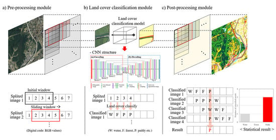
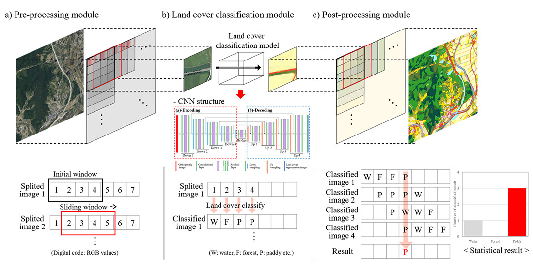
The land cover classification model converts HRRS images into land cover classification maps and the classification process goes through three basic modular phases (Figure 1). First, the HRRS images are inserted in the model by overlapping 75% of each image and then separated for each data to reflect different perspectives through a pre-processing module (Figure 1a). The separated images are then passed through a CNN-based land cover classification module. The module converts the data into a land cover map, which classifies land uses with trained colors (Figure 1b). Lastly, the land cover maps with different perspectives of a single region that was classified are aggregated in the post-processing module and the resulting image is printed as the final land use classification map (Figure 1c).

2.2. Pre-Processing Module

The land use classification through CNN model does not simply classify land uses by color values of pixels; it considers the spatial distribution of color values of the surrounding pixels for process. Using only a single image of the land for land use classification could increase errors in the classification process. The pre-processing module was applied to increase the accuracy of the land use classification, as it provides images of different perspectives.

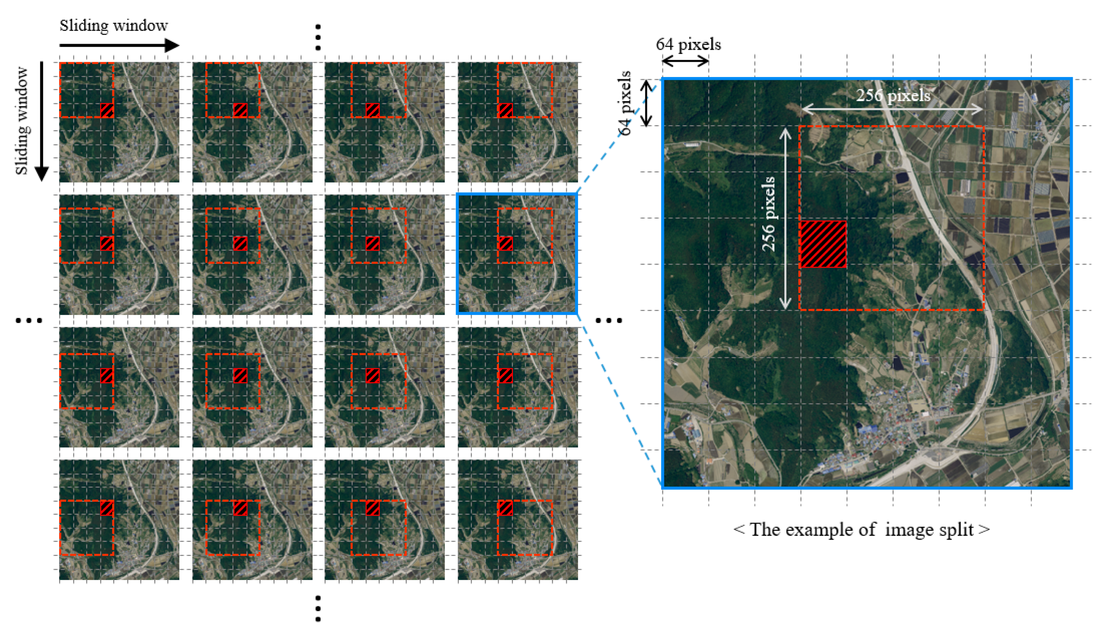
For the pre-processing module, the size of land use classification images to be separated from a random size orthographic image was set to 256 × 256 pixels considering the computer performance. Each image was 75% (shifting 64 pixels) overlapped both in the horizontal and vertical directions, and then separated for diversification of perspectives (Figure 2). Finally, images of 16 different perspectives were used to classify land uses in a single space (Figure 2, red hatched area).

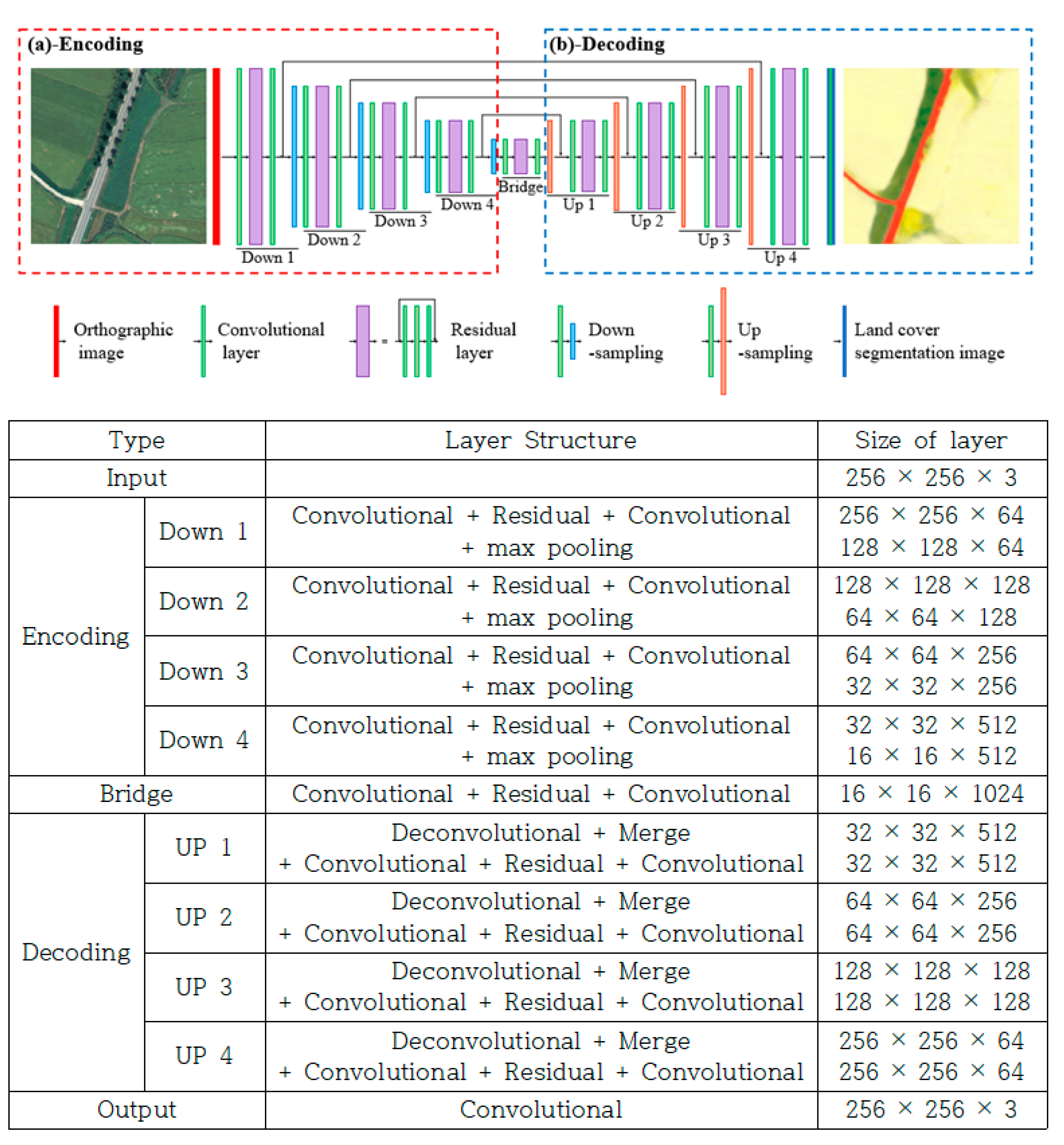
2.3. Architecture of CNN Based Land Cover Classification Module

The land cover classification module converts the input image into a land cover map, in which the land use status is segmented semantically by respective land cover color codes (please refer to

Table 1. Hierarchy of land cover categories and respective color codes (Environmental Geographic Information System (EGIS)).

Main Category (7 Items)	Parent Subcategory (22 Items)	Child Subcategory (41 Items)	Color Code
			R	G	B	Remark
Urbanized area	Residential area	Single housings	254	230	194
		Apartment housings	223	193	111
	Industrial area	Industrial facilities	192	132	132
	Commercial area	Commercial and office buildings	237	131	184
		Mixed use areas	223	176	164
	Culture and sports recreation area	Culture and sports recreation facilities	246	113	138
	Transportation area	Airports	229	38	254
		Ports	197	50	81
		Railroads	252	4	78
		Roads	247	65	42
		Other transportation and communication facilities	115	0	0
	Public facilities area	Basic environmental facilities	246	177	18
		Educational andadministrative facilities	255	122	0
		Other public facilities	199	88	27
Agricultural area	Paddy	Consolidated paddy filed	255	255	191
		Paddy field without consolidation	244	230	168
	Upland	Consolidated upland	247	249	102
		Upland without consolidation	245	228	10
	Greenhouse	Green houses	223	220	115
	Orchard	Orchards	184	177	44
	Other cultivation lands	Ranches and fish farms	184	145	18
		Other cultivation plots	170	100	0
Forest	Deciduous forest	Deciduous forests	51	160	44
	Coniferous forest	Coniferous forests	10	79	64
	Mixed forests	Mixed forests	51	102	51
Grassland	Natural grassland	Natural grasslands	161	213	148
	Artificial grassland	Golf courses	128	228	90
		Cemeteries	113	176	90
		Other grasslands	96	126	51
Wetland	Inland wetland	Inland wetlands	180	167	208
	Coastal wetland	Tidal flats	153	116	153
		Salterns	124	30	162
Barren lands	Natural barren	Beaches	193	219	236
		Riversides	171	197	202
		Rocks and boulders	171	182	165
	Artificial barrens	Mining sites	88	90	138
		Sports fields	123	181	172
		Other artificial barrens	159	242	255
Water	Inland watery	Rivers	62	167	255
		Lakes	93	109	255
	Marine water	Marine water	23	57	255

in Section 3.3.2). CNN was used for an effective image segmentation of the land cover, and FusionNet [36] of CNN, which separates cell from EM image [37,38] was conceptually similar to the creating land cover maps that identifies land use boundary using HRRS image, was used as the structure of the neural network.

The number of spectral channels used for the land classification was upgraded by adopting three channels: red (R), green (G), blue (B), of the HRRS image. The land cover classification result is expressed in values that are closest to the learned classification color for each land cover (Table 1).

The entire land cover classification module largely consists of two processes: encoding (Figure 3a) that classifies land use features from the image data, and decoding (Figure 3b) that prints the land use map classified through different colors according to the classified land use features. The module is configured with a combination of four basic layers of the convolutional layer, residual layer, down-sampling and up-sampling, and summation-based skip connection.

As a layer that is widely used in the deep learning field, the convolutional layer converts the entered data into compressed data including special information in the processes of convolution, activation function, and batch normalization [39]. Parameters used in the configuration of convolutional layer in this module are kernel size of 3, stride of 1, and padding of 1. In general, the rectified linear unit (ReLU) is used in the activation function (Equation (1)). However, in ReLU, the gradient value always becomes negative if the entered value is negative. Data compression using ReLU in the encoding process could result in data losses. Leaky ReLU, which can provide gradient value when the input value is negative, can complement ReLU (Equation (2)). Therefore, the module was configured with Leaky ReLU as an activation function in the encoding process and ReLU as an activation function in the decoding process.

ReLU: f(x) = max(0, x)

(1)

Leaky ReLU: f(x) = max(0.01x, x)

(2)

The residual layer is configured with three convolutional layers and a single summation-based skip connection. The neural network deepens, and the data features become noticeable through the three convolutional layers included in the residual layer. However, as the neural network deepens, a gradient vanishing problem occurs. To solve this issue, we used the summation-based skip connection in the residual layer, which integrates the past data with the currently processing data in the module, and configured the layer to enable a more exquisite classification [36].

Down-sampling was used to reduce computation volume and prevent overfitting [40]. Maxpooling function that brings the largest value within each stride was also used. In the down-sampling process, a kernel size of 2, stride of 2, and zero padding were used. In contrast to the down-sampling, the up-sampling increases the layer size to acquire images segmented by colors from the land use classification results. The deconvolution function was used for up-sampling.

Summation-based skip connections, which solve the gradient vanishing issue and help the information transfer, were used in the residual layer and long skip connections. So, the convolutional layer could be much deeper to include more parameters without losing its training efficiency. Skip connections function to merge the previous layer and the current layer by summing the matrix of each layer. Short skip connections in residual layer add up first convolutional layer with third convolutional layer. Four long skip connections connect the layer of the encoding path to the decoding path, which are the same size.

2.4. Post-Processing Module

The primary function of post-processing integrates module is to analyze and integrate classified images of 16 different perspectives, produced from the pre-processing and the land cover classification modules, into a final land cover using numerical and statistical methods. The post-processing module consists of two parts of land cover assignment to a pixel level and following land cover integration to determine the final land cover to a given pixel.

Land cover assignment part is the process to determine land cover to a pixel based on the classified output. The R, G, B values of classified image pixels are the output by the classification model that were trained with land cover map color (label). The model output values do not match exactly to the reference values of land cover map since the trained CNN works only to minimize errors. The Gaussian distance was used to find nearest land cover to a given pixel by calculating the distance between the classified color values (result) with reference land cover code (label). The formula to calculate Gaussian distance is given in Equation (3). The label land cover with the lowest Gaussian distance was assigned to a given pixel.

Gaussin Distance = √ ((R_result − R_label)² + (G_result − G_label)² + (B_result − B_label)²),

(3)

where Rresult, Gresult, Bresult = red, green, blue values represent output produced by the land cover classification module and Rlabel, Glabel, Blabel = red, green, blue values indicate the reference values specific to each sub-category of land cover maps given in Table 1. The reference color code is standardized and provided by the Korean government.

The land cover integration is a process of aggregating the land cover classification results that are classified through images of 16 different perspectives of one region, to determine the final land cover classification result. The 16 different classification results per pixel that were obtained from the pre-processing, the land cover classification module, and the pixel land use determination process of the post-processing module were aggregated to produce the final result. The item selected as having the greatest number of land cover classification results among the aggregated land cover classification items was determined as the final land use classification result (Equation (4)). When the maximum counts are same for the different land covers, then one of them was chosen arbitrarily. The final land use classification result per pixel is printed as a final land cover classification map in which the classification of the aggregated orthographic image input is complete.

Classification Result = max(count_paddy, count_forest, count_water, count_item, etc.),

(4)

where count_item is the number of the classified item out of the total classification results.

3. Data Set and Methods for Verification of Land Cover Classification Model

3.1. Study Procedure

The schematics of the developed model training and verification is shown in Figure 4.

3.2. Study Area

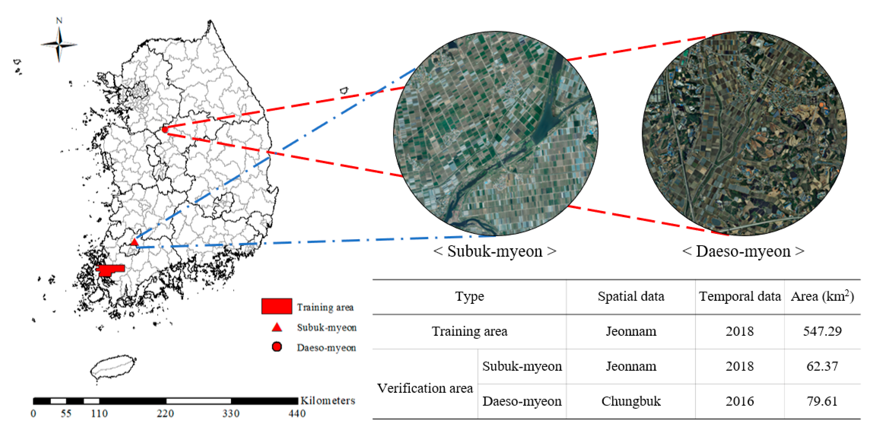
3.2.1. Training Area

To train the land cover classification model, a training area of 547.29 km² was selected, which could acquire the latest source data of 2018 and contain the largest cultivating area in South Korea. The selected area included a cultivated acreage of 22,495 ha in Yeongam-gun and 20,279 ha in Muan-gun, and is a useful area for training the model for agricultural land cover [41]. In addition, it could also train the model for urban land cover, as it includes the main urban areas, such as the Gun offices in Jeonnam province, Mokpo City Hall, etc., which are some of the major buildings in the urban center. The areas selected for the study are shown in Figure 5.

3.2.2. Verification Area

The artificial intelligence (AI) based land cover classification is likely to be the most accurate for data that have spatial and temporal dimensions similar to that of the training data. To increase the accuracy of model verification, this study selected two separate areas for the verification process; one area had spatial and temporal dimensions similar to that of the training area and the other area was located far from the training area and had different time periods.

An area of 62.37 km² in Subuk-myeon, Jeonnam province, in 2018 was selected as the first verification area. For the Subuk-myeon area, an orthographic image source data obtained for the same period as that of the study data (2018) exists, and spatially, it is located in the same region as the study data (Jeonnam province).

As the second verification area, an area of 79.61 km² in Daeso-myeon, Chungbuk province, in 2016 was selected. Daeso-myeon was selected because an orthographic image source data recorded at a different time period (2016) and located far from the study data was available. These two verification areas are shown in Figure 5.

3.3. Data Acquisition

3.3.1. Orthographic Image

The orthographic images of the study area (2018) and the verification areas (2018, 2016) were obtained from the National Geographic Information Institute (NGII). The orthographic images are produced through geometric correction and orthometric correction of aerial photographs recorded in each period. The spectral channels of HRRS image include the red, green, and blue bands. The resolution of the orthographic images of the established study area (2018) and verification areas (2018, 2016) is 51 cm/pixel.

3.3.2. Land Cover Map

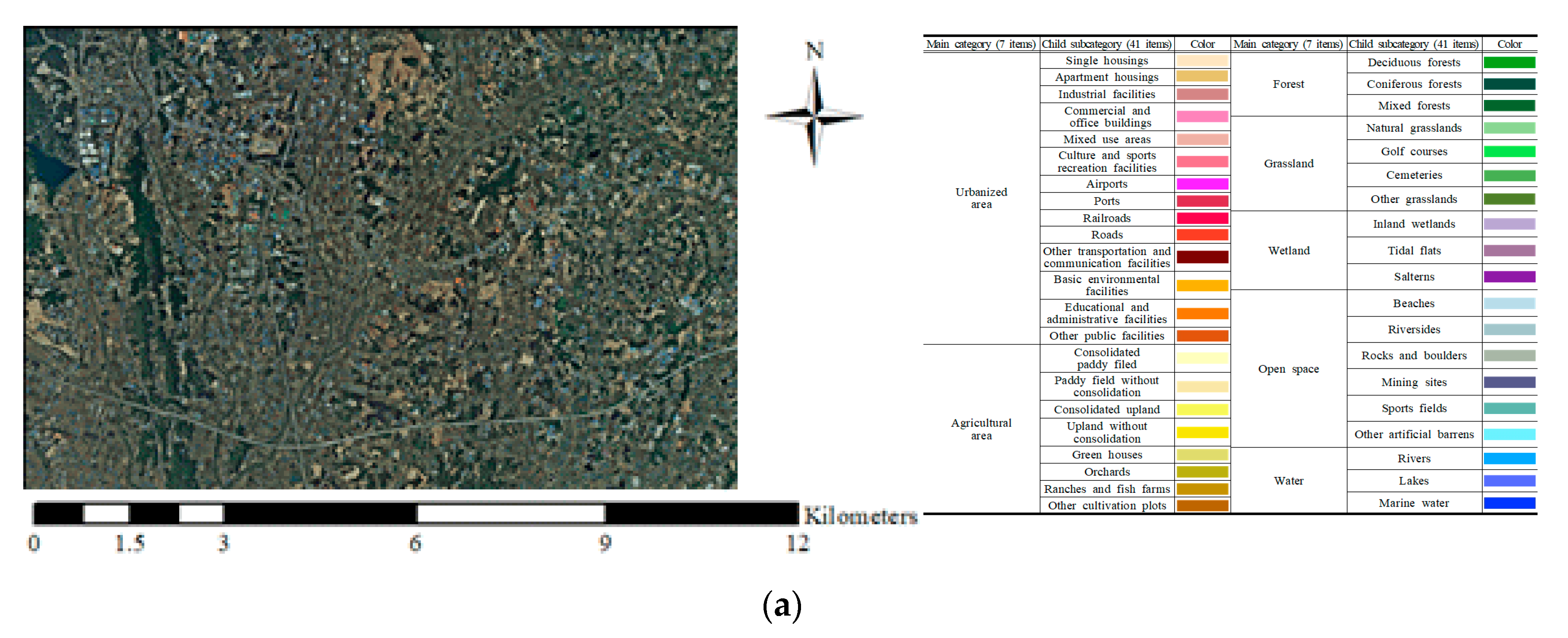
The land cover maps of the selected sites for model training (2018) and the two verification sites (2018, 2016) were established using the Korean Environmental Geographic Information System (EGIS). The land cover maps of EGIS are the results of on-screen digitizing of the orthographic images from the NGII by assigning various colors to respective land use types as shown in Table 1. It should be noted that the color codes were thoughtfully assigned that the sub-category-classes under a main category have similar color hues, i.e., red for urbanized area, yellow for agricultural land, dark green for forest, light green for grassland, violet for wetland, light blue for barren lands, and dark blue for water. The land cover map was used as the ground truth serving as the target for the supervised model training. As previously described in Equations (3) and (4), the color codes in Table 1 were also used for calculating the Gaussian distance for the land cover assignment to the pixel level. The land cover map is presented in three different categories based on the level of detail; seven items in the main category, 22 items in the parent subcategory, and 41 items in the child subcategory.

3.4. Training Land Cover Classification Model

The location adjustment of the established orthographic images and land cover maps of the study area was made using ArcMap (ESRI, Ver. 10.1). To train the land cover classification model, acquired data were split vertically and horizontally with 256 × 256 pixels (130 m × 130 m), which is an appropriate size for confirming the land uses. The land cover map classified by colors of the child subcategory (41 items) was used for the model training. A total of 32,384 orthographic images and 32,384 land cover maps of the same area were created.

For effective model training, an image augmentation process that increases the number of the study data was performed. The level of the diversification of the study data was increased by rotating the generated orthographic images and land cover maps at angles of 0°, 90°, 180°, and 270°. Finally, 129,536 sheets of each orthographic image and land cover map were used for training the model.

The model training was conducted using Intel i7-9700K CPU and NVIDA GeForce GTX 1060 6gb hardware, and using the Python (Ver. 3.6.8) and PyTorch (Ver. 1.0.1) software. Mean square loss (MSELoss) was used for estimating errors in the model, and the training was completed when the error value was less than 0.01. The training was completed with MSELoss value of 0.0077 after training 129,536 sheets of the established study data 84 times.

3.5. Verification Method for Land Cover Classification Model

The accuracy of the land cover classification was evaluated by creating accuracy metrics that indicated consistencies of items between the evaluation results of the two evaluators and by estimating the quantitative index values for overall accuracy and kappa coefficient based on the metrics.

The accuracy metrics were created by comparing the land cover classification map created by the on-screen digitizing method (reference land cover) with that created classified by the developed model (classified land cover). The consistent land cover classification results of both evaluators (reference land cover, classified land cover) were indicated on the diagonal matrix of accuracy metrics.

Producer’s accuracy and user’s accuracy show the ratio of correctly matched area of each land use in reference data and classified data, respectively (Equations (5) and (6)). The overall accuracy was estimated using Equation (7), which indicates the ratio of the correctly classified land cover area to the entire area. Three accuracy indicator has values ranging from 0 to 1, and the classification becomes more accurate as this value comes closer to 1. Although the overall accuracy enables an intuitive accuracy evaluation of the land cover classification, it has a limitation of not being able to consider a possibility of accidentally assigning the same land cover classification for different areas.

Thus, a kappa coefficient, which excluded the probability of accidental consistency in the overall accuracy, was also used in the accuracy evaluation of the land cover classification. The kappa coefficient means a value compared with a randomly arranged accuracy metrics (Equation (8)). The kappa coefficient has values ranging from −1 to 1, and as the value gets closer to 1, the classification attains a higher accuracy. Model performance was evaluated by the strength criteria provided by Landis and Koch [42].

Producer’s accuracy = x_ij/x_i+

(5)

User’s accuracy = x_ij/x_+j

(6)

Overall accuracy = (Σ(i = 1 to k) (x_ii))/N

(7)

Kappa coefficient = (N x (Σ(i = 1 to k) (x_ii)) − (Σ(i = 1 to k) (x_i+ x x_+j)))/(N² − (Σ(i = 1 to k) (x_i+ x x_+j)))

(8)

where i and j represents each row and column, respectively, and N denotes total number of the classification result.

4. Verification Result of Land Cover Classification Model

4.1. Performance of Land Cover Classification at the Child Subcategory

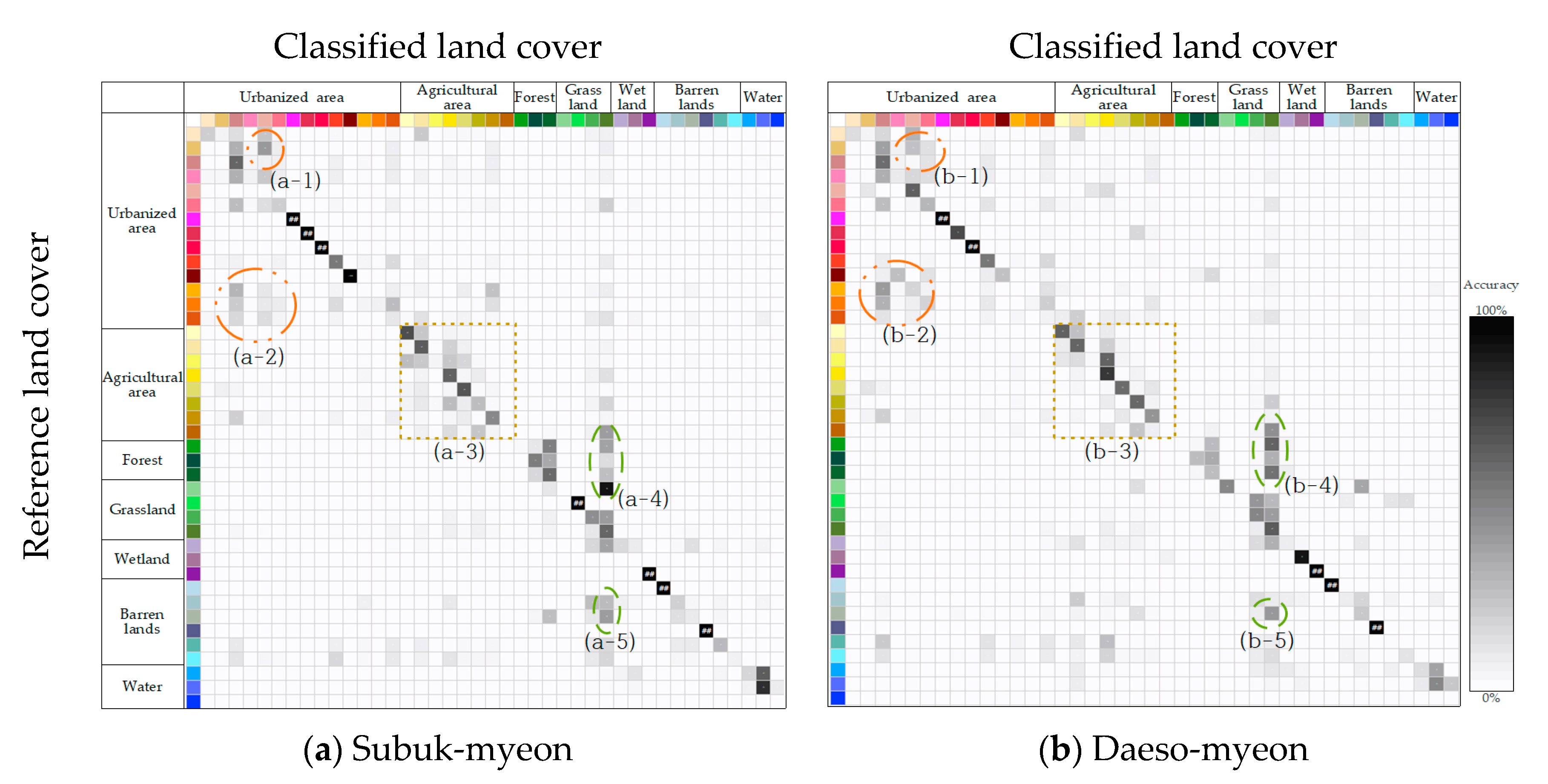
Model performance in land cover classification for the respective Subuk-myeon (Jeonnam province, 2018) and Daeso-myeon (Chungbuk province, 2016) was presented in terms of the number of classified land cover that matches with the reference land label as shown in Figure 1. A total of 41 land covers at the child subcategory level were classified with the developed model (Figure 6). As can be seen from the darker gray along the diagonal direction, the developed model performed reasonably well in land cover classification. Overall, the model demonstrated better accuracy for the urban, agriculture, forest and water areas, while relatively poor in grass, wetlands, and barren lands showing the wider spectrum of classified land covers.

Most of misclassifications at the child subcategory (41 classes) level occurred within the main categories (seven classes) for the urbanized and agriculture areas. It can be seen that some sporadic points are deviated from the diagonal line, but it still remains within the same square of the respective main land cover classes in Figure 6. Several urban land covers in the 41-classes-subcategory are buildings which are similar in appearance so making it difficult for the developed model differentiate its usage, for example among apartment, industrial, and commercial buildings as shown in Figure 6(a-1,a-2,b-2 and b-2). Agricultural areas also include land cover sub-classes with similar outward shapes depending on consolidation that resulted in the misclassifications within the main category (Figure 6(a-3,b-3)).

However, grass and barren lands showed the wider misclassifications over the main land cover categories. Many of grass lands were misclassified by the forest, wetlands, and barren lands, of which appearances are similar as natural landscapes (Figure 6(a-4,a-5,b-4, and b-5)).

The statistics of 16 different perspective classifications are presented in Figure 7. As aforementioned, the final land cover classification was assigned statistically based on the maximum counts of a given land cover class.

The greater the maximum count is, the more consistent the developed model performed for a given class. The average counts for urban, agriculture, forest, and water land covers were greater than 14, which indicates approximately 87% consistency of out of 16 classifications. This implies also that the consideration of viewpoints could improve classification consistency by reducing 13% potential errors as compared to a single-pixel based classification. Consistent with Figure 6, the maximum counts for wetland and barren lands were smaller than nine, which means nearly half of these categories could be misclassified as other land covers if the 16 different perspective classifications were not implemented. Thus the 16-perspective application can increase model accuracy by improving the model classification consistency.

4.2. Classification Accuracy of the Aggregated Land Cover to Main Category

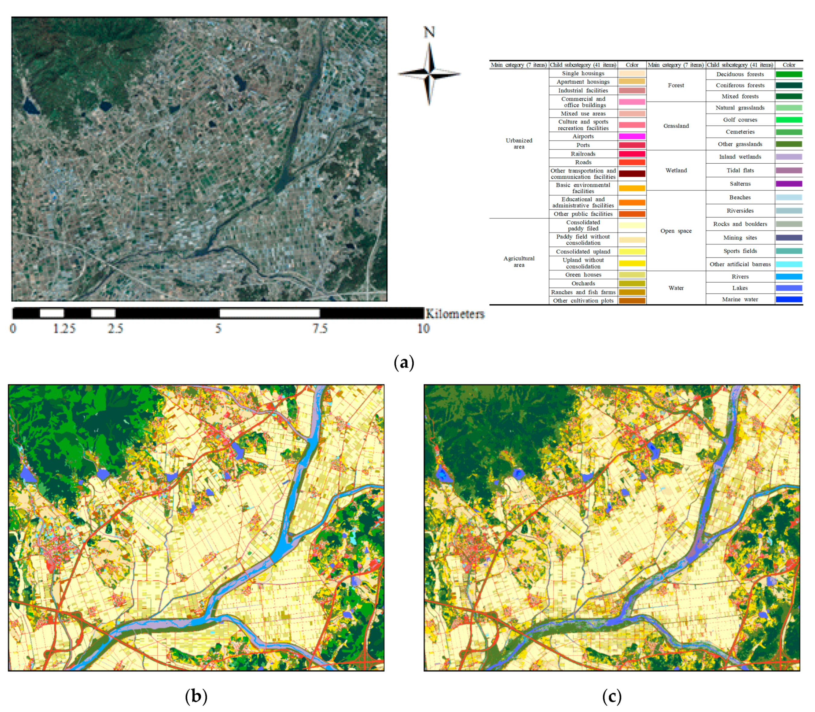
The overall accuracy of the land cover classification was evaluated by expanding the printed land uses of child subcategory unit to the main category unit. A land cover map (Figure 8c) of an orthographic image (Figure 8a) of Subuk-myeon which is spatially and temporally similar to the study area (Jeonnam province, 2018) was printed through the land cover classification model developed in this study. This result is compared with the land cover map (Figure 8b) obtained from EGIS and the accuracy metrics are presented in

Table 2. Accuracy metrics and verification indices for the Subuk-myeon area (unit: 1000 pixels).

		Classified Land Cover								Producer’s Accuracy (%)
		Urbanized Area	Agricultural Area	Forest	Grassland	Wetland	Barren Lands	Water	Total
Reference land cover	Urbanized area	18,658	2834	19	1850	41	193	24	23,619	79.00
	Agricultural area	4439	114,426	61	5848	177	1122	114	126,187	90.68
	Forest	83	329	29,198	9619	4	24	3	39,261	74.37
	Grassland	2148	4870	1414	23,920	424	853	43	33,672	71.04
	Wetland	138	309	22	3840	1595	1205	352	7461	21.38
	Barren lands	1369	802	13	879	13	385	9	3469	11.10
	Water	29	22	1	153	688	187	5055	6133	82.41
	Total	26,864	123,593	30,728	46,108	2943	3970	5600	239,804	-
User’s Accuracy (%)		69.45	92.58	95.02	51.88	54.20	9.70	90.27	-	-
Overall accuracy		0.81
Kappa Value		0.71

.

Visual comparison of both the land cover map of EGIS and the land cover map produced by the model shows an overall match between the two maps. However, the result showed large differences in the green areas of deciduous forests, coniferous forests, and mixed forests that were classified as the forest area. The classification of the overall forest area showed users accuracy of 95.02% and a producer’s accuracy of 74.37%. This high accuracy result was achieved because the developed model is effective in classifying forest and other areas; however, it is not as effective in identifying detailed forest types within the forest area. As the forest area has large differences in elevations, the shades developed are based on its terrain, which affects the colors of the orthographic images. Such differences in colors made it difficult to classify the forests in detail.

The qualitative index of overall accuracy and kappa coefficient were 0.81 and 0.71, respectively. This showed a substantial degree of accuracy with the kappa coefficient ≥0.6 and <0.8. It was confirmed that this was an improvement when compared to overall accuracy of 73.7% and kappa coefficient of 0.69 [43] of the land cover classification using an object-based algorithm in the agricultural region.

Agricultural area, forest area and water showed high classification accuracy. The user’s accuracy and producer’s accuracy of each classification item from the accuracy metrics showed in agricultural area (92.58%, 90.68%), forest area (95.02%, 74.37%), and water (90.27%, 82.41%), respectively. However, the classification accuracy of grassland (51.88%, 71.04%), wetlands (54.20%, 21.38%), and barren lands (9.70%, 11.10%) were low. It was caused by the misclassification of grassland to forest, wetland to grassland and barren lands, and barren lands to wetland and agricultural area.

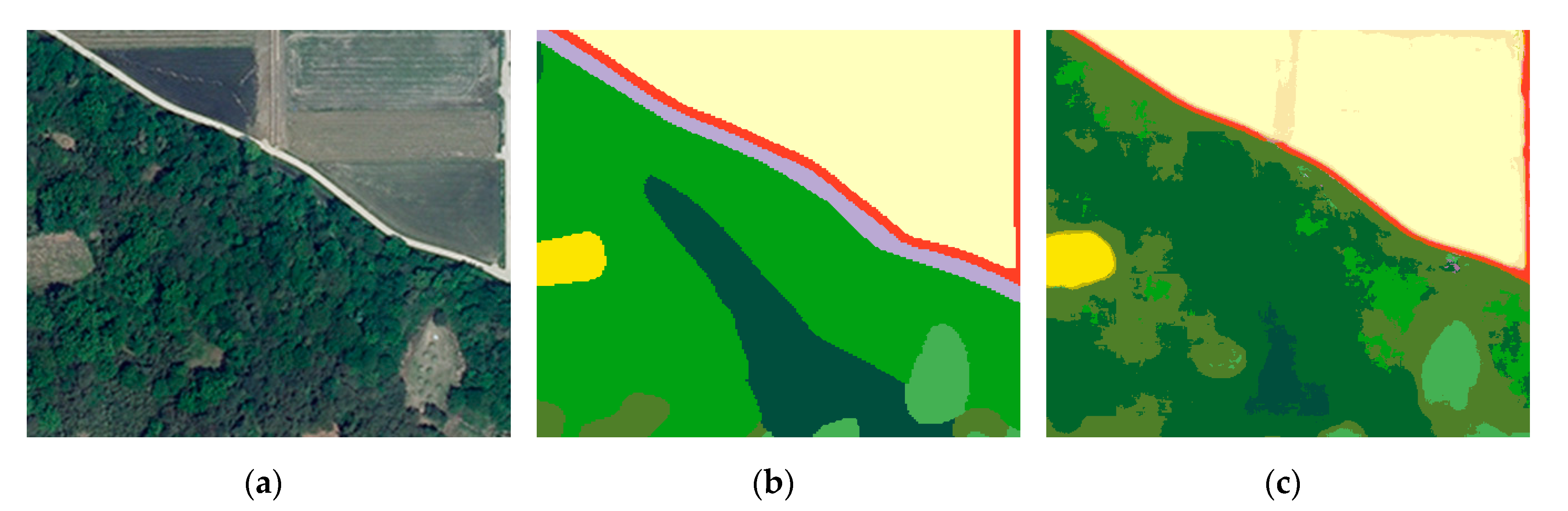
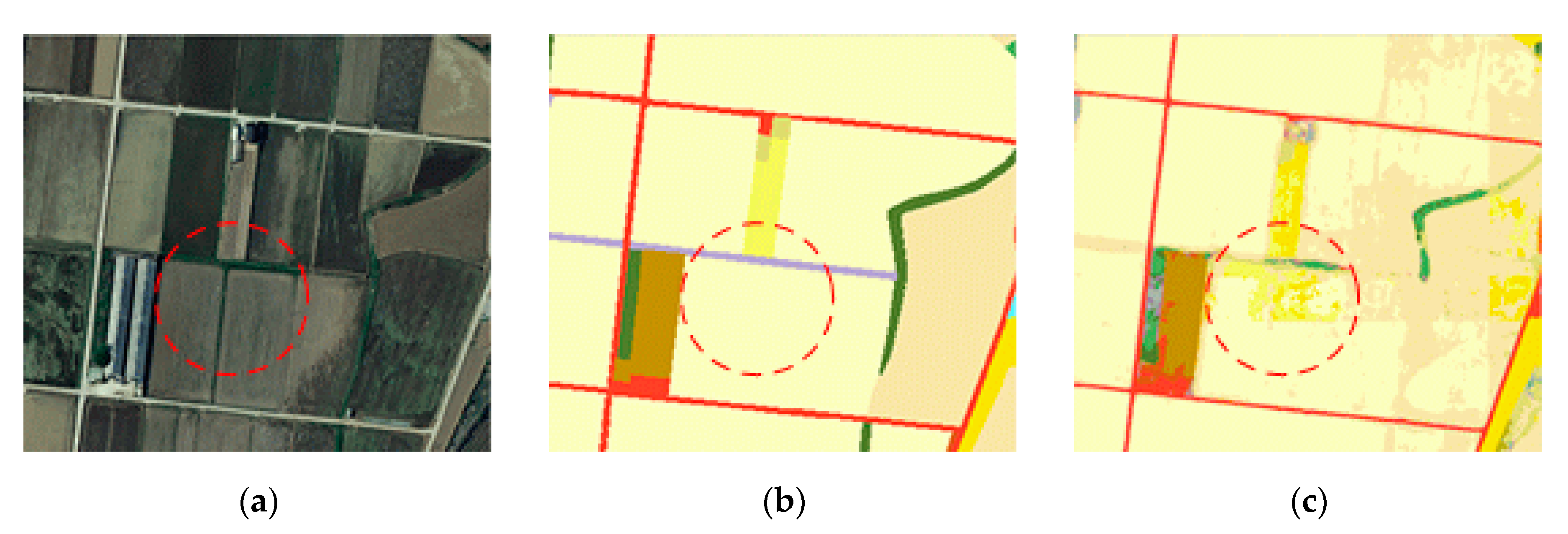
This might be results from the ambiguity of the land cover, which causes difficulties in classification, as the forms of land uses are not clear (Figure 9 and Figure 10).

Most of the forest area in the orthographic image (Figure 9a) was defined as deciduous forest (Figure 9b, bright green) and coniferous forest (Figure 9b, dark green). However, the developed model classified mostly as mixed forest (Figure 9c, intermediate dark green) and grass lands (Figure 9c, yellowish green). As mentioned, this might be due to difficulties of distinguish these two classes and thus more intensive training on forest areas are needed to increase the accuracy.

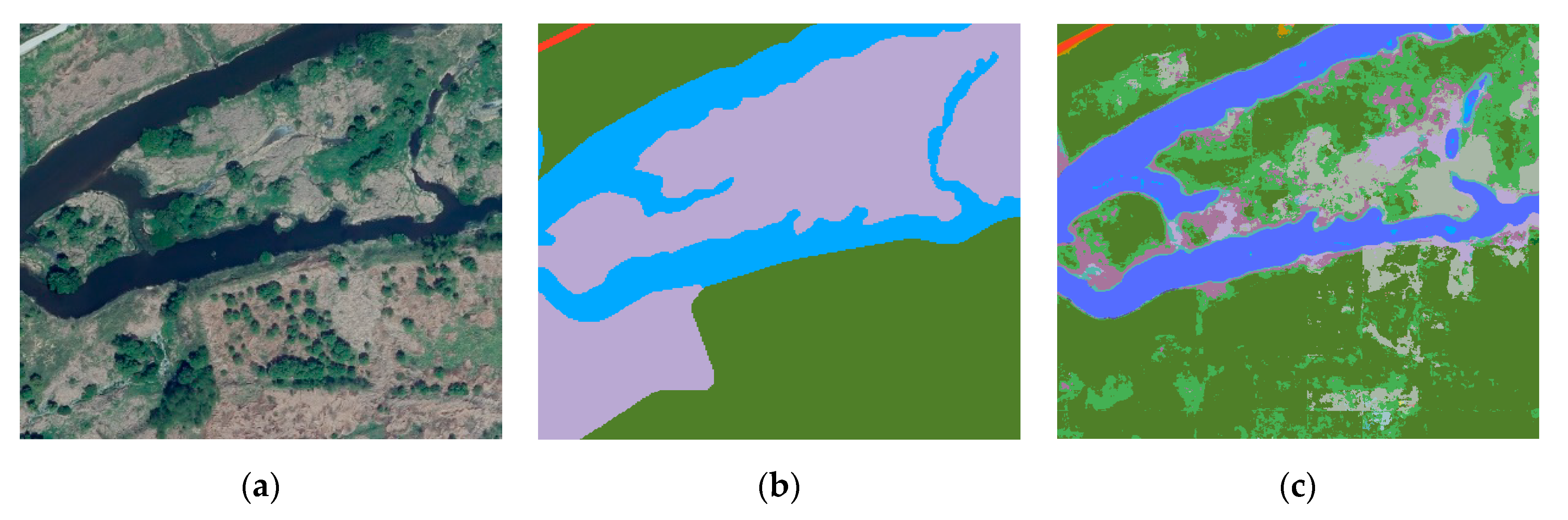
In the space surrounded by the central river of the orthographic image (Figure 10a) near the river in Subuk-myeon, it is difficult to clearly classify the wetlands, barren lands, and grasslands by visual reading. In the land cover map (Figure 10b) of EGIS, this was classified as a single land use (wetland) based on the land boundary, while in the land cover classification model, the classification of an optimal land use per pixel (Figure 10c) was conducted. The differences in the land cover classification results caused by the ambiguity of the land cover largely affected the classification accuracy of wetlands and barren lands.

Wetlands are generally located in lower land area and thus pooled water during rainy season, while grasslands and barren lands are dry lands with and without vegetation, respectively. Thus wetlands, grasslands, and barren lands could share the similar landscape and its land cover changes depending on the existence of water and vegetation. This may have caused some ambiguity among those land covers that resulted in relatively poor performance. The ambiguity can be alleviated if additional indicators of NDWI (normalized difference water index) and NDVI (normalized difference vegetation index) are used, along with the RGB values.

Additionally, the overall portions of wetland and barren areas are relatively small as compared to other land covers, so the model might have been under-trained. The poor performance for water and barren area would be improved by training the model with more data specific to these land covers.

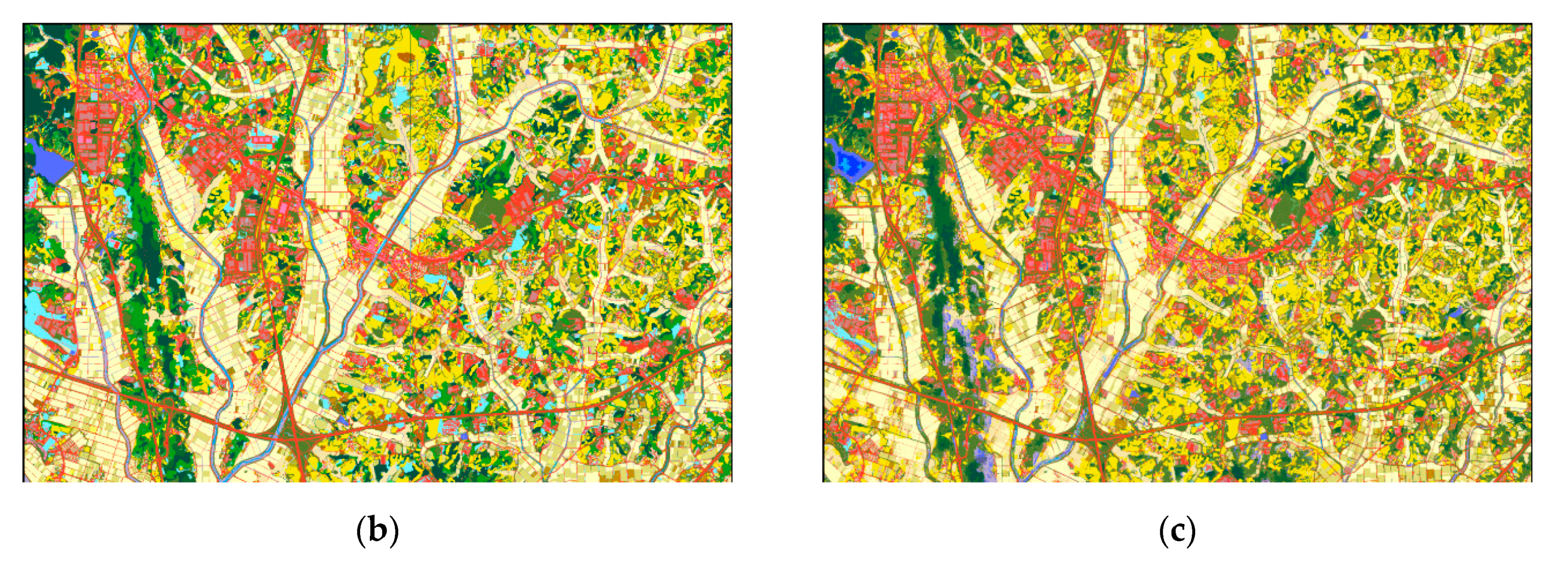
Figure 11 shows the orthographic image of Daeso-myeon (Figure 11a), which is spatially (Chungbuk province) and periodically (2016) different from the study area (Jeonnam province, 2018) and the land cover map (Figure 11c) classification produced by the land cover classification model. The accuracy metrics obtained by verifying it visually with the land cover map of EGIS (Figure 11b) are presented in

Table 3. Accuracy metrics and verification indices of the Daeso-myeon area (unit: 1000 pixels).

		Classified Land Cover								Producer’s Accuracy (%)
		Urbanized Area	Agricultural Area	Forest	Grassland	Wetland	Barren Lands	Water	Total
Reference land cover	Urbanized area	44,614	4451	25	4026	203	334	68	53,721	83.05
	Agricultural area	6759	124,749	254	6677	334	737	402	139,912	89.16
	Forest	214	469	14,582	18,109	1184	213	198	34,970	41.70
	Grassland	3951	7333	775	39,064	815	788	344	53,069	73.61
	Wetland	558	2327	5	3985	759	790	77	8501	8.92
	Barren lands	3956	3483	14	2,702	131	2280	38	12,604	18.09
	Water	73	321	2	378	280	249	2012	3315	60.69
	Total	60,125	143,132	15,657	74,941	3706	5392	3139	306,093	-
User’s Accuracy (%)		74.20	87.16	93.13	52.13	20.47	42.29	64.10	-	-
Overall accuracy		0.75
Kappa Value		0.64

.

Although the verification area was both spatially and periodically different from the study area, it was confirmed that the classification was conducted well when visually comparing the land cover map of EGIS with the land cover map produced by the model.

In particular, the qualitative index of overall accuracy and kappa coefficient were 0.75, and 0.64, respectively. When compared with the Subuk-myeon area (overall accuracy of 0.81, kappa coefficient of 0.71), which was similar to the study area, it showed approximately 10% lower accuracy. However, it showed a substantial degree of accuracy with kappa coefficient ≥ 0.6 and < 0.8. This result confirms the possibility of applying the land cover classification of a general orthographic image data regardless of its acquired time, or space. As for the classification accuracy of each item, the results for agricultural area (user’s accuracy of 87.16%, producer accuracy of 89.16%) were accurate, whereas the results for wetlands (user’s accuracy of 20.47%, producer’s accuracy of 8.92%) and barren lands (user’s accuracy of 42.29%, producer’s accuracy of 18.09%) showed a lower level of accuracy. Thus, it can be confirmed that the results are similar to those from the aforementioned verification of Subuk-myeon.

4.3. Land Cover Classification of the Agricultural Fields

Agricultural land cover data is widely used in various purpose from rural hydrological analysis to soil conservation to irrigation planning. To this end, further investigation in agricultural lands were conducted by analyzing the parent level land cover. The model simulation results from the Daeso-myeon, which is one of the verification areas, was evaluated by estimating the classification accuracy to the level of subcategory land cover including paddy field, upland, and greenhouses.

Agricultural lands (equivalent to the second row and column in Table 3) were extracted from the global simulation results and rearranged based on the subcategories as presented in

Table 4. Classification results of paddy field, upland, and green house in Daeso-myeon (unit: 1000 pixels).

		Classified Land Cover							Producer’s Accuracy (%)
		Paddy	Upland	Green House	Orchard	Other Cultivation Lands	Other Land Cover	Total
Reference land cover	Paddy	56,560	7523	1073	130	27	2262	67,575	83.70
	Upland	2340	36,944	589	1743	286	5129	47,031	78.55
	Green house	557	359	9908	491	1575	3828	16,718	59.27
	Orchard	9	158	6	1356	84	624	2236	60.66
	Other cultivation lands	99	417	261	875	1378	3321	6352	21.70
	Other land cover	4302	6556	1398	3156	2971	147,798	166,181	88.94
	Total	63,868	51,956	13,236	7751	6322	162,961	306,093
User’s accuracy (%)		88.56	71.11	74.86	17.50	21.80	90.70	-	-
Overall accuracy		0.83
Kappa Value		0.73

. All other land cover classes other than agricultural lands were lumped into other land cover class. The model performance in agricultural lands were evaluated with overall accuracy and kappa coefficient were also estimated.

The land cover classification in the agricultural field showed an overall accuracy of 0.83 and kappa coefficient of 0.73, which showed the result of substantial. In evaluating the accuracy per item, the classification of paddy (user’s accuracy of 88.56, producer’s accuracy of 83.70) and upland (user’s accuracy of 71.11 producer’s accuracy of 78.55) showed a higher level of accuracy. In both items, some paddy fields were misclassified as upland and some uplands as paddy fields. This arises from an ambiguity in boundaries that occurs when classifying the land cover in pixel unit, which is a characteristic of the model (Figure 12).

In reality, the land uses of paddy field and upland are in the form of parcels with boundaries. However, the result of the model produces the optimal land cover classification per pixel not per parcel with boundaries. As indicated by the red dotted lines shown in Figure 12, most of the area is classified as paddy field in the classification of a parcel of paddy field, whereas some part of the area is classified as upland. The ambiguity in boundaries could be improved to additional process of applying land parcel boundaries into pixel-based land cover.

The classification of the greenhouses had a user’s accuracy of 74.86 and a producer’s accuracy of 59.27, and, therefore, some areas were classified as upland. After the structure of the green house was demolished, it showed a similar land use characteristic to upland in the orthographic image, although it was classified as green house in the land cover map of EGIS.

The classification accuracy of orchards and other cultivation plots was evaluated to be lower than that of the other items. The land cover map of EGIS classifies areas of cultivating garden trees, street trees, etc., other than fruit trees and livestock production facilities, as other cultivation lands. However, the ambiguity in classification of orchards and other cultivation lands that cultivate garden trees, street trees, etc., and greenhouses and other cultivation lands that were used as livestock production facilities became a limitation factor.

5. Conclusions

As an effort to improve the update of land cover map especially for agriculture, this study developed the land cover classification model using the CNN-based FusionNet network structure, and verified its applicability for the two areas of different spatial and temporal characteristics.

The land cover classification model was designed to perform an accurate land cover classification by reflecting the adjacent land uses based on CNN. In addition, by reading 16 images of different perspectives for the land cover classification of a single area, the classification consistency was increased.

Performance of the developed model was reasonably good demonstrating the overall accuracies of 0.81 and 0.75, and kappa coefficients of 0.71 and 0.64, respectively. However, the accuracy for wetlands and barren lands were 26.24% and 20.30%, which were substantially misclassified to grassland and wetland, respectively. These areas were relatively small and, thus, further training with data specific to these land covers may improve the accuracy.

When considering only agricultural areas, the model performance was better showing overall accuracy of 0.83 and kappa coefficients of 0.73. Moreover, each land cover classification accuracy of paddy field, upland was 80.48% on average.

It was concluded that the developed model can enhance the efficiency of the current slow process of land cover classification and thus assist rapid update of land cover map.

The developed CNN-based land cover classification model classifies land cover on a pixel unit, which can be different from the actual land use of parcel unit. So, considering land parcel boundaries into pixel-based land cover can improve the classification accuracy substantially and thus will be further studies in the future.

References

- Blasi, C.; Zavattero, L.; Marignani, M.; Smiraglia, D.; Copiz, R.; Rosati, L.; Del Vico, E. The concept of land ecological network and its design using a land unit approach. Plant Biosyst. 2008, 142, 540–549. [Google Scholar] [CrossRef]
- Yang, J.; Chen, F.; Xi, J.; Xie, P.; Li, C. A multitarget land use change simulation model based on cellular automata and its application. Abstr. Appl. Anal. 2014, 2014, 1–11. [Google Scholar] [CrossRef] [Green Version]
- He, T.; Shao, Q.; Cao, W.; Huang, L.; Liu, L. Satellite-observed energy budget change of deforestation in northeastern China and its climate implications. Remote Sens. 2015, 7, 11586–11601. [Google Scholar] [CrossRef] [Green Version]
- Anderson, M.C.; Allen, R.G.; Morse, A.; Kustas, W. Use of Landsat thermal imagery in monitoring evapotranspiration and managing water resources. Remote Sens. Environ. 2012, 122, 50–65. [Google Scholar] [CrossRef]
- Schilling, K.E.; Jha, M.K.; Zhang, Y.K.; Gassman, P.W.; Wolter, C.F. Impact of land use and land cover change on the water balance of a large agricultural watershed: Historical effects and future directions. Water Resour. Res. 2008, 44, 44. [Google Scholar] [CrossRef]
- Rahman, S. Six decades of agricultural land use change in Bangladesh: Effects on crop diversity, productivity, food availability and the environment, 1948–2006. Singap. J. Trop. Geogr. 2010, 31, 254–269. [Google Scholar] [CrossRef] [Green Version]
- Bontemps, S.; Arias, M.; Cara, C.; Dedieu, G.; Guzzonato, E.; Hagolle, O.; Inglada, J.; Matton, N.; Morin, D.; Popescu, R.; et al. Building a data set over 12 globally distributed sites to support the development of agriculture monitoring applications with Sentinel-2. Remote Sens. 2015, 7, 16062–16090. [Google Scholar] [CrossRef] [Green Version]
- Borrelli, P.; Robinson, D.A.; Fleischer, L.R.; Lugato, E.; Ballabio, C.; Alewell, C.; Bagarello, V. An assessment of the global impact of 21st century land use change on soil erosion. Nat. Commun. 2017, 8, 1–13. [Google Scholar] [CrossRef] [Green Version]
- Kyungdo, L.; Sukyoung, H.; Yihyun, K. Farmland use mapping using high resolution images and land use change analysis. Korean J. Soil Sci. Fertil. 2012, 45, 1164–1172. [Google Scholar]
- Song, X.; Duan, Z.; Jiang, X. Comparison of artificial neural networks and support vector machine classifiers for land cover classification in Northern China using a SPOT-5 HRG image. Int. J. Remote Sens. 2012, 33, 3301–3320. [Google Scholar] [CrossRef]
- Lee, H.-J.; Lu, J.-H.; Kim, S.-Y. Land cover object-oriented base classification using digital aerial photo image. J. Korean Soc. Geospat. Inf. Syst. 2011, 19, 105–113. [Google Scholar]
- Sakong, H.; Im, J. An empirical study on the land cover classification method using IKONOS image. J. Korean Assoc. Geogr. Inf. Stud. 2003, 6, 107–116. [Google Scholar]
- Enderle, D.I.; Weih, R.C., Jr. Integrating supervised and unsupervised classification methods to develop a more accurate land cover classification. J. Ark. Acad. Sci. 2005, 59, 65–73. [Google Scholar]
- Laha, A.; Pal, N.R.; Das, J. Land cover classification using fuzzy rules and aggregation of contextual information through evidence theory. IEEE Trans. Geosci. Remote Sens. 2006, 44, 1633–1641. [Google Scholar] [CrossRef] [Green Version]
- Jin, B.; Ye, P.; Zhang, X.; Song, W.; Li, S. Object-oriented method combined with deep convolutional neural networks for land-use-type classification of remote sensing images. J. Indian Soc. Remote Sens. 2019, 47, 951–965. [Google Scholar] [CrossRef] [Green Version]
- Paisitkriangkrai, S.; Shen, C.; Av, H. Pedestrian detection with spatially pooled features and structured ensemble learning. IEEE Trans. Pattern Anal. Mach. Intell. 2016, 38, 1243–1257. [Google Scholar] [CrossRef] [Green Version]
- Roy, M.; Melgani, F.; Ghosh, A.; Blanzieri, E.; Ghosh, S. Land-cover classification of remotely sensed images using compressive sensing having severe scarcity of labeled patterns. IEEE Geosci. Remote Sens. Lett. 2015, 12, 1257–1261. [Google Scholar] [CrossRef]
- Prasad, S.V.S.; Savitri, T.S.; Krishna, I.V.M. Classification of multispectral satellite images using clustering with SVM classifier. Int. J. Comput. Appl. 2011, 35, 32–44. [Google Scholar]
- Huang, X.; Zhang, L. An SVM ensemble approach combining spectral, structural, and semantic features for the classification of high-resolution remotely sensed imagery. IEEE Trans. Geosci. Remote Sens. 2012, 51, 257–272. [Google Scholar] [CrossRef]
- Kang, M.S.; Park, S.W.; Kwang, S.Y. Land cover classification of image data using artificial neural networks. J. Korean Soc. Rural Plan. 2006, 12, 75–83. [Google Scholar]
- Kang, N.Y.; Pak, J.G.; Cho, G.S.; Yeu, Y. An analysis of land cover classification methods using IKONOS satellite image. J. Korean Soc. Geospat. Inf. Syst. 2012, 20, 65–71. [Google Scholar]
- Schöpfer, E.; Lang, S.; Strobl, J. Segmentation and object-based image analysis. Remote Sens. Urban Suburb. Areas 2010, 10, 181–192. [Google Scholar]
- Längkvist, M.; Kiselev, A.; Alirezaie, M.; Loutfi, A. Classification and segmentation of satellite orthoimagery using convolutional neural networks. Remote Sens. 2016, 8, 329. [Google Scholar] [CrossRef] [Green Version]
- Kamilaris, A.; Prenafeta-Boldú, F.X. A review of the use of convolutional neural networks in agriculture. J. Agric. Sci. 2018, 156, 312–322. [Google Scholar] [CrossRef] [Green Version]
- Gavade, A.B.; Rajpurohit, V.S. Systematic analysis of satellite image-based land cover classification techniques: Literature review and challenges. Int. J. Comput. Appl. 2019, 1–10. [Google Scholar] [CrossRef]
- Luus, F.P.S.; Salmon, B.P.; Bergh, F.V.D.; Maharaj, B.T. Multiview deep learning for land-use classification. IEEE Geosci. Remote Sens. Lett. 2015, 12, 2448–2452. [Google Scholar] [CrossRef] [Green Version]
- Santoni, M.M.; Sensuse, D.I.; Arymurthy, A.M.; Fanany, M.I. Cattle race classification using gray level co-occurrence matrix convolutional neural networks. Procedia Comput. Sci. 2015, 59, 493–502. [Google Scholar] [CrossRef] [Green Version]
- Chen, Y.; Lin, Z.; Zhao, X.; Wang, G.; Gu, Y. Deep learning-based classification of hyperspectral data. IEEE J. Sel. Top. Appl. Earth Obs. Remote. Sens. 2014, 7, 2094–2107. [Google Scholar] [CrossRef]
- Lee, S.H.; Chan, C.S.; Wilkin, P.; Remagnino, P. Deep-plant: Plant identification with convolutional neural networks. In Proceedings of the 2015 IEEE International Conference on Image Processing (ICIP), Quebec City, QC, Canada, 27–30 September 2015. [Google Scholar]
- Grinblat, G.L.; Uzal, L.C.; Larese, M.G.; Granitto, P.M. Deep learning for plant identification using vein morphological patterns. Comput. Electron. Agric. 2016, 127, 418–424. [Google Scholar] [CrossRef]
- Kussul, N.; Lavreniuk, M.; Skakun, S.; Shelestov, A. Deep learning classification of land cover and crop types using remote sensing data. IEEE Geosci. Remote Sens. Lett. 2017, 14, 778–782. [Google Scholar] [CrossRef]
- Fu, G.; Liu, C.; Zhou, R.; Sun, T.; Zhang, Q. Classification for high resolution remote sensing imagery using a fully convolutional network. Remote Sens. 2017, 9, 498. [Google Scholar] [CrossRef] [Green Version]
- Lu, H.; Fu, X.; Liu, C.; Li, L.-G.; He, Y.-X. Cultivated land information extraction in UAV imagery based on deep convolutional neural network and transfer learning. J. Mt. Sci. 2017, 14, 731–741. [Google Scholar] [CrossRef]
- Carranza-García, M.; García-Gutiérrez, J.; Riquelme, J. A framework for evaluating land use and land cover classification using convolutional neural networks. Remote Sens. 2019, 11, 274. [Google Scholar] [CrossRef] [Green Version]
- Pan, S.; Guan, H.; Chen, Y.; Yu, Y.; Gonçalves, W.; Junior, J.M.; Li, J. Land-cover classification of multispectral LiDAR data using CNN with optimized hyper-parameters. ISPRS J. Photogramm. Remote Sens. 2020, 166, 241–254. [Google Scholar] [CrossRef]
- Quan, T.M.; Hildebrand, D.G.; Jeong, W.K. Fusionnet: A deep fully residual convolutional neural network for image segmentation in connectomics. arXiv 2016, arXiv:1612.05360. [Google Scholar]
- Ronneberger, O.; Fischer, P.; Brox, T. U-net: Convolutional networks for biomedical image segmentation. In International Conference on Medical Image Computing and Computer-Assisted Intervention; Springer: Cham, Switzerland, 2015; pp. 234–241. [Google Scholar]
- Çiçek, Ö.; Abdulkadir, A.; Lienkamp, S.S.; Brox, T.; Ronneberger, O. 3D U-Net: Learning dense volumetric segmentation from sparse annotation. In Proceedings of the International Conference on Medical Image Computing and Computer-Assisted Intervention, Athens, Greece, 17–21 October 2016; Volume 9901, pp. 424–432. [Google Scholar]
- Shang, W.; Sohn, K.; Almeida, D.; Lee, H. Understanding and improving convolutional neural networks via concatenated rectified linear units. In Proceedings of the International Conference on Machine Learning, New York, NY, USA, 19–24 June 2016; pp. 2217–2225. [Google Scholar]
- Zeiler, M.D.; Fergus, R. Stochastic pooling for regularization of deep convolutional neural networks. arXiv 2013, arXiv:1301.3557. [Google Scholar]
- Cultivated Area by City and County in 2017 from Kostat Total Survey of Agriculture, Forestry and Fisheries. Available online: http://kosis.kr/statHtml/statHtml.do?orgId=101&tblId=DT_1EB002&conn_path=I2 (accessed on 27 September 2020).
- Landis, J.R.; Koch, G.G. The measurement of observer agreement for categorical data. Biometrics 1977, 33, 159–174. [Google Scholar] [CrossRef] [Green Version]
- Kim, H.O.; Yeom, J.M. A study on object-based image analysis methods for land cover classification in agricultural areas. J. Korean Assoc. Geogr. Inf. Stud. 2012, 15, 26–41. [Google Scholar] [CrossRef] [Green Version]
Figure 1.
Conceptual schematic of the land cover classification model. (a) Pre-processing module, (b) Land cover classification module, (c) Post-processing module.
Figure 2.
Scheme of the 16 perspectives preparation of the pre-processing module. The red hatched is the target classification area from the 16 different viewpoints.
Figure 3.
Architecture of the convolutional neural network (CNN)-based land cover classification module. (a) Encoding, (b) Decoding.
Figure 4.
Schematics of the study procedure.
Figure 5.
Study areas for the model training and verification.
Figure 6.
Model performance matrices for (a) the Subuk-myeon and (b) Daeso-myeon areas. The accuracy was presented in gray scale based on the percentage of the classified pixels that batch with the reference land cover label to the total number of pixels. The darker gray indicates the more pixels were classified to the given land cover. Refer to the color codes for detailed land cover given Table 1.
Figure 7.
Average counts for different land covers from the 16 different perspective classifications.
Figure 8.
Photos of (a) Orthographic image, (b) land cover map, and (c) classification results of the Subuk-myeon area.
Figure 9.
Example of ambiguity of land cover in grassland (yellowish green and whitish green is grass land, other greens are forest with different types of tree, yellows are agricultural area, and red is road). (a) Orthographic image, (b) Land cover map, (c) Classification result.
Figure 10.
Example of ambiguity of land cover in wetland and barren lands (purple is wetland, gray is barren lands, green is grass land, blue is river, red is road). (a) Orthographic image 1, (b) Land cover map 1, (c) Classification result 1.
Figure 11.
Photos of (a) Orthographic image, (b) land cover map, and (c) classification results of the Daeso-myeon area.
Figure 12.
Example of ambiguity of boundaries (bright and dark skin color are paddy field, bright and dark yellow are upland). (a) Orthographic image, (b) Land cover map, (c) Classification result.