Technical Note

Image Collection Simulation Using High-Resolution Atmospheric Modeling

1
NGA/Research, National Geospatial-Intelligence Agency, Springfield, VA 22150, USA
2
Brookhaven National Laboratory, Upton, NY 11973, USA
3
NGA/A, National Geospatial-Intelligence Agency, Springfield, VA 22150, USA
*
Author to whom correspondence should be addressed.
Remote Sens. 2020, 12(19), 3214; https://0-doi-org.brum.beds.ac.uk/10.3390/rs12193214
Submission received: 27 August 2020 / Revised: 28 September 2020 / Accepted: 29 September 2020 / Published: 1 October 2020
(This article belongs to the Special Issue Feature Papers of Section Atmosphere Remote Sensing)

Abstract

:
A new method is described for simulating the passive remote sensing image collection of ground targets that includes effects from atmospheric physics and dynamics at fine spatial and temporal scales. The innovation in this research is the process of combining a high-resolution weather model with image collection simulation to attempt to account for heterogeneous and high-resolution atmospheric effects on image products. The atmosphere was modeled on a 3D voxel grid by a Large-Eddy Simulation (LES) driven by forcing data constrained by local ground-based and air-based observations. The spatial scale of the atmospheric model (10–100 m) came closer than conventional weather forecast scales (10–100 km) to approaching the scale of typical commercial multispectral imagery (2 m). This approach was demonstrated through a ground truth experiment conducted at the Department of Energy Atmospheric Radiation Measurement Southern Great Plains site. In this experiment, calibrated targets (colored spectral tarps) were placed on the ground, and the scene was imaged with WorldView-3 multispectral imagery at a resolution enabling the tarps to be visible in at least 9–12 image pixels. The image collection was simulated with Digital Imaging and Remote Sensing Image Generation (DIRSIG) software, using the 3D atmosphere from the LES model to generate a high-resolution cloud mask. The high-resolution atmospheric model-predicted cloud coverage was usually within 23% of the measured cloud cover. The simulated image products were comparable to the WorldView-3 satellite imagery in terms of the variations of cloud distributions and spectral properties of the ground targets in clear-sky regions, suggesting the potential utility of the proposed modeling framework in improving simulation capabilities, as well as testing and improving the operation of image collection processes.

Graphical Abstract

1. Introduction

The simulation of image collection for airborne and satellite sensors has many applications. Simulated video and image products make it possible to measure the value of potential imagery collections before they are carried out. Accurate simulations can help mission planners use collection platforms more efficiently, safely, and effectively, and predict the detection and visibility of targets and other scene features under anticipated collection conditions [1,2]. Simulation is useful for prototyping sensors [3] and for testing algorithms in the imaging chain [4]. Simulation can be used to predict, analyze, and reverse engineer artifacts and system issues that degrade image and video quality. Simulations can generate large quantities of annotated training data for computer vision machine learning systems.
The research described in this article is concerned with passive remote sensing in visible and near-infrared spectral bands. Some researchers have generated synthetic scenes using emulations of physical effects modeled on input images [5]. However, the main goal of this project was to create end-to-end 3D simulations of image collection that included all the scene features, such as the target, atmosphere, and sensor characteristics. The simulations must also include time-stepping to account for target motion, changes in ambient illumination, sensor platform motion, and atmospheric dynamics.
Several image collection simulation tools have been developed for this purpose, such as the Digital Imaging and Remote Sensing Image Generation (DIRSIG) model [1,2,3,4,6] and Monte Carlo Scene (MCScene) [7,8,9,10]. DIRSIG and MCScene account for scene features and sensor specifications well in many cases but do not account for dynamical, heterogeneous atmospheric effects at high spatial resolution. Both DIRSIG and MCScene accept, as input, collection platform and trajectory parameters, atmospheric parameters, and target parameters and generate an output of simulated images by simulating photon scattering from the target and through the atmosphere. It is possible to specify the spectral properties of ground targets and target scenes, and to include sensor design features in the models, but the atmosphere is generally treated as an unchanging feature with no spatial or temporal variations. Furthermore, there is no model that ingests existing weather data in real time, conducts high-resolution processing, and simulates potential imagery resulting from impending weather conditions. These are significant shortcomings, because atmosphere and weather are often the primary and most unpredictable factors that contribute to image quality degradation.
Weather conditions applied to image processing, correction, or simulation are generally homogeneous parameters, because atmospheric data have not been available that have the spatial scale of most imagery. When ambient weather conditions are used as parameters for correcting or calibrating imagery, single parameters for temperature, etc. may be applied to an entire scene of tens of square kilometers. This spatial scale is much coarser than the resolution scale of image data, which can be 1–4 m for a standard commercial satellite multispectral image.
Advanced weather modeling and increasing computing resources have improved the resolution of weather simulation. Large-eddy simulation (LES) explicitly resolves clouds and energetic turbulent eddies at fine scale (10–100 m) by calculating atmospheric dynamics and physics. LES has been increasingly applied to simulations of more realistic atmospheric conditions by constraining model inputs (which include aerosol size distribution parameters, hygroscopicity parameters, large-scale forcing and surface forcing) with locally measured boundary conditions and global- or regional-scale, low-resolution weather data [11].
It is worth considering the feasibility of applying high-resolution weather information to image collection simulations. The possible advantages include a more accurate spectral characterization of ground targets, more accurate measurement of temperature in thermal data, and better prediction of atmospheric impediments to imaging, such as clouds, haze, hail, sleet, and aerosols, that might influence satellite or airborne tasking decisions.
The concept of operation for this idea is that the weather model is represented as a 3D voxel grid placed over the scene. At each time step, LES calculations produce a new voxel grid for each parameter of interest, such as the cloud water content, droplet radius, humidity, temperature, and pressure. The image collection simulation accounts for the high-resolution weather data by masking or otherwise demarcating cloudy regions in the simulated imagery output. This process makes it possible to account for the high-spatial-resolution variability of effects from clouds and other atmospheric phenomena across a scene.
Section 2 of this article explains the method of image collection simulation and describes a ground truth experiment in which real imagery was collected. Section 2 also describes the process of developing a computer model of the 3D scene and calibrating the computer model to the physical properties of the scene. Section 3 explains the high-resolution atmospheric simulation. Section 4 describes the results of the image collection simulation, and Section 5 provides conclusions and possible paths for future work.

2. Materials and Methods

2.1. Image Collection Simulation Using DIRSIG

The purpose of image and video collection simulation is to account for all possible factors in the end-to-end image chain that can degrade video and image quality, and to be able to reproduce and explain artifacts or target signatures. The main factors to simulate include platform characteristics such as the camera specs, wavelength bands, sensor response functions, spectral linewidth, timing, jitter, altitude, and elevation and azimuth angles. The target factors include the reflectance, bidirectional reflectance distribution function (BRDF), and material composition of the facets. The atmosphere and environmental factors include the sun direction, temperature, moisture, haze, clouds, precipitation, and downwelling and upwelling radiation. The product of the image collection simulation is an image expressed in units of radiance. Video can be simulated as a concatenation of image frames collected at typical video rates.
The software package used in this paper was DIRSIG, which is a radiation transfer simulation program designed by the Carlsen Lab in the Rochester Institute of Technology [1,2,3,4]. DIRSIG simulates image collection by ingesting a computer-aided design (CAD) scene for which all the objects and environmental features have been assigned spectral characteristics. DIRSIG can be set up to use the Air Force Research Lab program MODTRAN to calculate atmospheric radiative transfer to supplement the target photon scattering and sensor response functions simulated by DIRSIG [12]; MODTRAN accepts an input formatted description of atmospheric characteristics, and outputs line-of-sight spectral transmittances and radiances calculated by solving the radiative transfer equation to account for absorption, emission, and scattering. DIRSIG models sensor characteristics in great detail, such as the sensor response at specific wavelengths and camera specifications. DIRSIG also models platform motion and trajectory, and moving objects on the ground [1,2].
DIRSIG and MODTRAN have been used for a long time to measure radiance transfer through the atmosphere and simulate the effects on imagery. However, existing image collection simulations in the open scientific literature cannot accommodate atmospheric dynamics with high spatial or temporal resolution [13]. Therefore, we developed an image collection simulation that includes the dynamical effects of the atmosphere on radiation transfer.

2.2. Ground Truth Experiment Using WorldView-3 Satellite Imagery
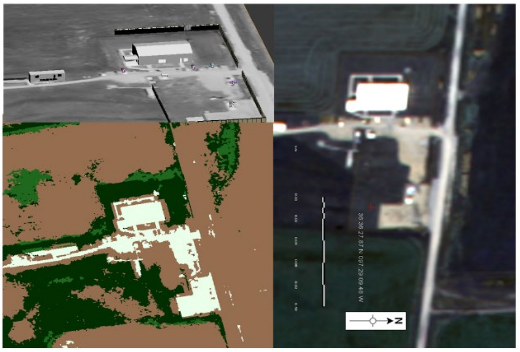
To test the validity of the image collection simulation, WorldView-3 commercial satellite images of the Atmospheric Radiation Measurement Southern Great Plains (ARM/SGP) site in Lamont, OK, were obtained. The images studied in this experiment were collected on 21, 22, 26, 27, and 28 May (Table 1). The satellite image data set includes visible spectral bands ranging from blue to red, infrared bands ranging from near infrared (NIR) to shortwave infrared (SWIR), and atmospheric sounding data from the Cloud, Aerosol, Water Vapor, Ice, Snow (CAVIS) instrument. Each image data set consisted of 15–17 files including multispectral, atmospheric, panchromatic, NIR, and SWIR bands. (See Supplementary Materials).
The cloud cover during the period ranged from nearly clear to overcast conditions. In several cases, the images had slight opacity from haze or thin cloud layers, which was ideal for testing the image collection simulation with atmospheric dynamics.
Calibration objects consisting of colored tarps were placed on the ground (Figure 1 and Figure 2). Two sites in the SGP central facility were used for the placing objects: a site at the north end of the compound and another to the south. The reflectance of the calibration tarps was later measured in a laboratory at the National Ground Intelligence Center (NGIC), as described in Appendix A. The calibration process helped to align the spectral characteristics of the DIRSIG scene model with the real-world imagery.

2.3. CAD Model

A CAD model of the ARM/SGP site (Figure 3) was built with Blender [14], an open source CAD software package. Existing CAD building models developed for the ARM/SGP site in FBX, DWG, and SQLITE formats were imported as input into Blender, and other objects in the scene were manually generated. The scene was draped onto a Digital Elevation Model (DEM), which also had a layer corresponding to terrain type, e.g., soil, grass, rock, etc. Vegetation and other simple scene objects were manually generated in Blender and added to the CAD model. The output of Blender is a 3D CAD model in a proprietary format that can be read by DIRSIG.
An annotated map of the vegetation and terrain types was derived from Google Maps imagery and a United States Department of Agriculture (USDA) model, CropScape, which provided ground truth values for the terrain classifications (soil, grass, etc.) [15]. A segmentation image product of the terrain classification was developed for the Google Maps imagery using a K-means unsupervised training model in the Harris Corporation ENVI software, so the image pixels in the Google Maps imagery could be assigned material values that could be mapped onto the CAD model. This process made it possible to combine the existing CAD model, which only included manmade buildings, equipment, and features, with an annotated background, thus providing material characteristics for the entire CAD model, which could be assigned spectra. The spectra of scene vegetation and other background objects were assigned from the Nonconventional Exploitation Factors Data System (NEFDS) database [16]. The spectra of target objects were derived from laboratory measurements of the BRDF. This terrain classification map of the scene was used by the DIRSIG model to simulate the reflectivity properties of the objects in the scene. The objects in the Blender model were exported into OBJ and GLIST formats; the latter is used by DIRSIG to assemble groups of objects into a scene.

2.4. WorldView-3 Simulation

The image collection was simulated in DIRSIG by modeling the trajectory of the WorldView-3 satellite. The following satellite parameters were extracted from the WorldView-3 XML metadata: the altitude, image dimensions, mean azimuth angle, and mean elevation angle. The ground sampling distance (GSD), or image resolution, was taken from the WorldView-3 metadata; the WorldView-3 GSD values ranged from 1.3 to 2.6 m, and the simulated GSD values were set to match the GSD values in the metadata. Other features of the camera model such as the pixel pitch, focal length, and aperture were unavailable but were able to be approximated from first-principle optics, based on knowledge of the image resolution and other parameters in the metadata.
The imaging bands used by WorldView-3, which ranged from coastal blue to SWIR, were used in the DIRSIG sensor model. The DIRSIG wavelengths used in the cloud fraction comparisons below were only the visible wavelengths, which were set as 450, 550, and 650 nm for blue, green, and red, respectively. This can be compared to the sensor bands WorldView-3 uses for red (630–690 nm), green (510–580 nm), and blue (450–510 nm). The laboratory spectra that were measured for the calibration tarps (Appendix A) were ingested into the DIRSIG model of the scene.

2.5. Atmospheric Model

The atmospheric model used in the image collection simulation is the Weather Research and Forecasting (WRF) model version 3.8.1 [17], which adopts a fully compressible equation system as a dynamical solver as well as advanced physics packages for subgrid-scale processes. For a flexible LES configuration, we utilized the version enhanced by implementing initialization, forcing, and statistics modules [11]. The LES model produces a time-stepping 3D distribution of atmospheric state variables, such as the pressure, temperature, water vapor, and cloud variables, as well as a variety of other statistical variables, which can be utilized as an input atmospheric model (i.e., 3D atmospheric data) for the image collection simulation.
The 3D grid of the LES was set to a spatial scale of 100 m in the horizontal direction and 30 m in the vertical direction below 5 km. The vertical grid spacing increases with height between 5 km and 15 km at the model top. When the 3D atmosphere is ingested into the image collection simulation, it is resampled in the vertical direction to a constant spatial interval of 30 m. The model domain consists of 144 × 144 × 226 grid boxes, which is an area of 14.4 by 14.4 km on the ground, and 15 km vertically. The dynamical time step is 0.5 sec. Periodic boundary conditions are applied for lateral boundaries.
The simulation uses the following physics packages: Thompson cloud microphysics [18], Rapid Radiative Transfer Model for General Circulation Models (RRTMG) radiative transfer [19], and 1.5-order Turbulence Kinetic Energy (TKE) subgrid-scale turbulence [20]. The Thompson scheme is a bulk cloud microphysics scheme that calculates evolutions and interactions of cloud hydrometeors in the categories of cloud liquid, cloud ice, rain, snow, and graupel; the RRTMG scheme calculates radiative transfer and heating due to longwave and shortwave fluxes based on the correlated k-distribution method [21,22,23]; the 1.5-order TKE scheme represents diffusion due to subgrid-scale turbulence based on the turbulent kinetic energy predicted based on wind shear, buoyancy, or external forcing [24,25,26].
The simulations were performed for each of five days on which the WorldView-3 images were collected. The model was initialized with a sounding profile at 12 UTC (6 local time) and was driven for 15 h. The simulation applies large-scale and surface forcing from the ARM VARANAL product [27], which is based on a variational analysis using rawinsondes, ground measurements at ARM/SGP, and National Oceanic and Atmospheric Administration (NOAA) Rapid Refresh (RAP) analysis data as input. To prevent the drift of simulated fields from VARANAL fields, a relaxation of the thermodynamic profile is applied using a 12 h time scale.

3. Results

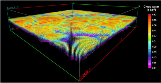
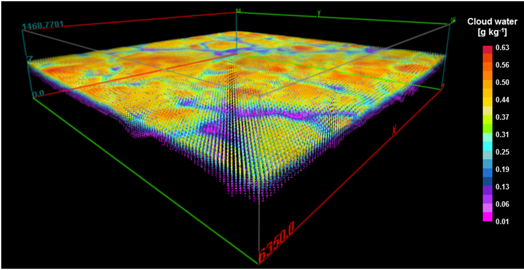
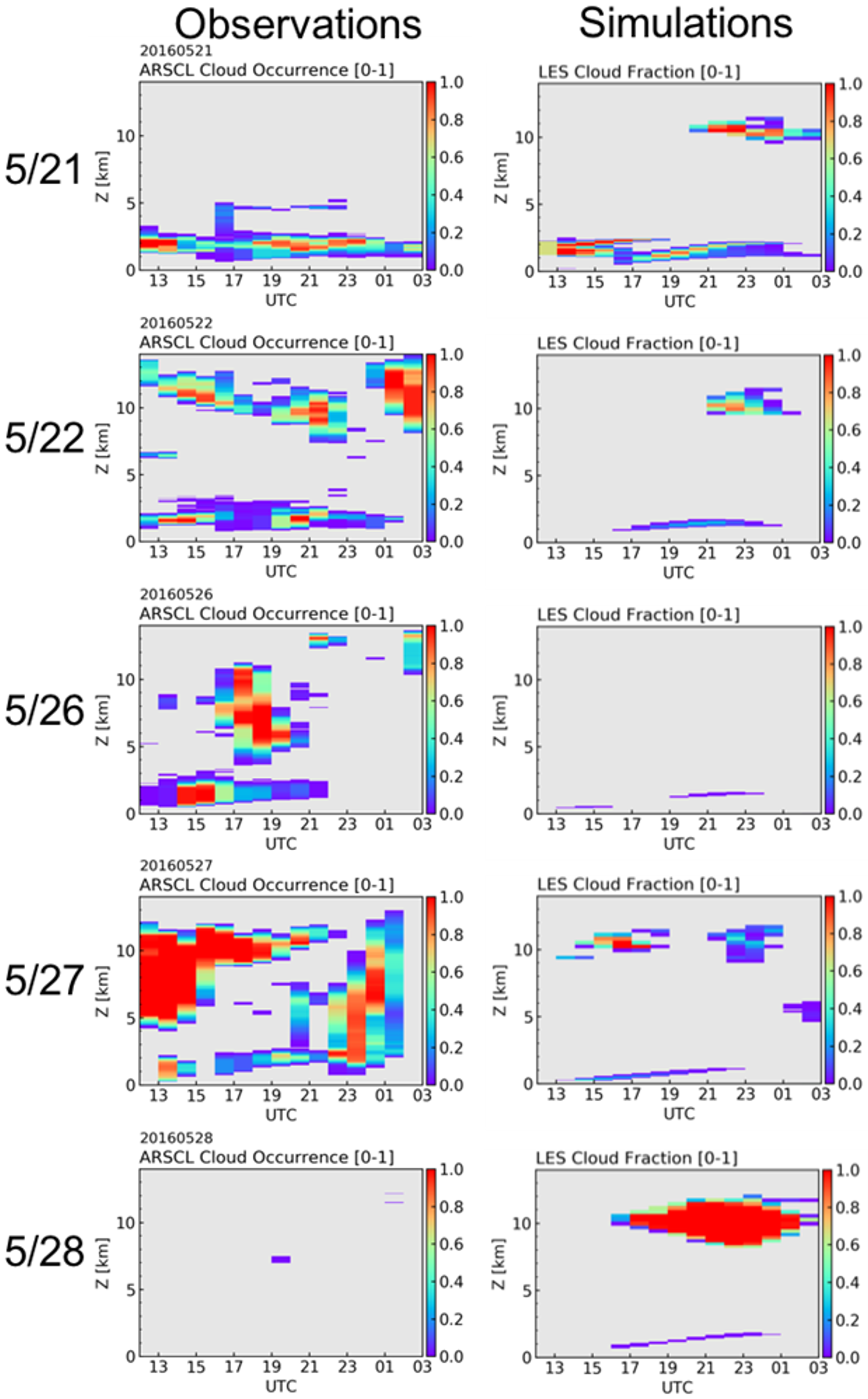
3.1. Comparison of Cloud Measurements and LES Atmospheric Simulation

First, we tested the quality of the time-stepping atmospheric model data. The simulated cloud fields were compared to observed cloud occurrence from the Active Remote Sensing of Clouds (ARSCL) product [28], which is based on vertically pointing radar and lidar at the ARM/SGP site. Figure 4 shows cloud occurrences from the ARSCL measurements and LES atmospheric simulation for the period of 21, 22, and 26–28 May. The cloud occurrence was hourly averaged to reduce the scale mismatch between the 1D measurement and the 3D simulation. The simulations generally captured the observed peaks of cloud layers at the lower and upper levels. The observations and simulations generally show that the clouds with more coverage also generally occupied more height and had a longer duration during the course of the day. For specific times and heights, the simulated clouds could be overpredicted (e.g., upper-level clouds on 21 May) or underpredicted (e.g., upper-level clouds on 22 May). The larger difference at upper levels suggest that the quality of the simulation could be improved by better large-scale forcing and ice microphysics, which are responsible for the cloud generation at the upper levels.
We performed several tests to examine the simulation’s sensitivities to the choice of microphysics scheme and relaxation time scale (not shown). By switching from Thompson microphysics to Morrison microphysics [29], upper-level cloud occurrence and duration increased in most cases.
Lower-level clouds were almost identical in the two simulations using different microphysics schemes. With a reduced relaxation time scale (i.e., stronger relaxation), the simulated clouds were more persistent at lower levels but were diminished at upper levels. The sensitivity tests produced mixed results depending on the different times, heights, and case days. Since parameter tuning for each case is not preferable for operational purposes and for prototyping the framework, we used simulations with a combination of Thompson microphysics and a 12 h relaxation time scale for the following analysis, and planned a separate study for more consistent improvements.

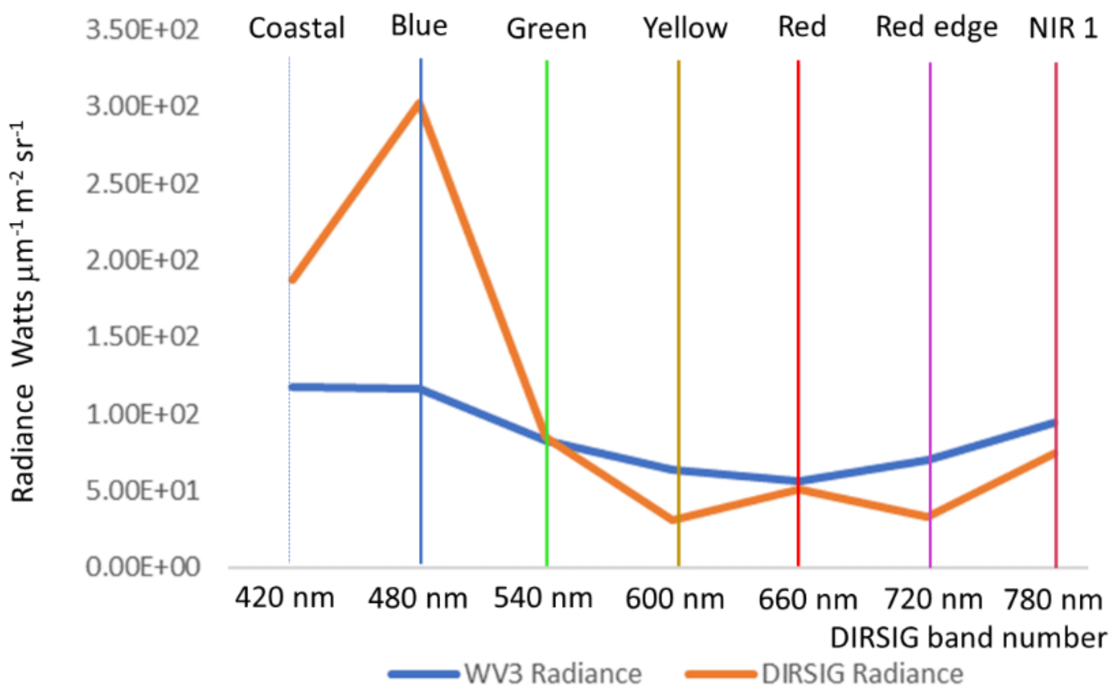
3.2. Comparison of Image Collection Simulation and Satellite Ground Truth

Next, the image collection simulation was performed with DIRSIG using the LES high-resolution atmosphere and modeled 3D scene at ground level, and it was evaluated with a ground truth experiment using WorldView-3 satellite images. This procedure was performed according to the following steps:
  • Run the LES models using the forcing data taking into account the SGP site observations during the period of the ground truth experiment.
  • For the five days and times when imagery was collected at the SGP (Table 1 and Table 2), capture the 3D atmosphere, particularly the cloud water.
  • Align the 3D atmosphere with the scene as projected onto a 2D ground plane.
  • Integrate the cloud water along parallel lines of sight extending from each ground pixel to the satellite’s position for each day.
  • These integrated lines of sight form a cloud mask (Figure 5), and the cloud coverage percentage is the percent of pixels for which clouds obscure the line of sight.
Table 2 compares the cloud coverage from the image collection simulation to the cloud coverage reported in the metadata of the WorldView-3 images. Unlike the previously shown comparison with ARSCL (Figure 4), the cloud coverage here is derived from image collection simulations that consider the target-to-sensor angle and field of view of the WorldView-3 satellite measurements. The results for the simulated cloud coverage agree with the WorldView-3 cloud coverage within 23% for all days except 26 May. The WorldView-3 image on 26 May had 99% cloud cover, and the atmospheric model missed the clouds completely. Since the upper-level stratiform clouds are dependent on the input large-scale forcing rather than model dynamics, the discrepancy is likely due to the insufficient quality of the input forcing data. A possible mitigation for the forcing uncertainty would be to use regional-scale simulations that incorporate more observational data to constrain the simulations. Using multiple sets of LES forcing data and driving multiple LES simulations would also be useful for quantifying the potential uncertainty of the forcing data.
Examples of DIRSIG simulations that include the high-resolution atmospheric modeling are shown in Figure 5. The currently used modeling framework simulates small-scale clouds and turbulence structures for given large-scale meteorological conditions. Thus, the simulations are not designed to capture the physical location, size, or structure of individual clouds but to capture the cloud statistics such as the fractional coverage and the effects on visibility. The colors in the simulations represent classes of objects (grass, dirt, etc.). The simulated images on the left in these figures were not formed to match the red–green–blue colors as the WorldView-3 images on the right, but the spectral properties of the cloud-free areas in the DIRSIG products were calibrated to match the spectra of the WorldView-3 image products across as many bands as possible in the wavelength range from coastal blue to short-wave infrared. A description of this process is provided in Appendix A.
We generated spectral plots over the range of the WorldView-3 imagery wavelengths (420–830 nm). Figure 6 shows the DIRSIG simulation radiance values, which include the spectra of the NGIC lab measurements of tarp reflectance, compared to the radiance values measured on the tarp in the WorldView-3 image from 22 May. The radiance values from the WorldView-3 image represent average values from 3–4 samples obtained with the ENVI image viewer [13]. The agreement of measurements is good for green and red but worse for the blue band.
Though DIRSIG is unable to calculate cloud radiometry, it is possible to use the atmospheric simulation to calculate the lower bounds of visibility, by integrating the 3D cloud water. The extinction coefficient σext determines the range of visibility Sm, which can be calculated, assuming a constant extinction coefficient across the visible light spectrum, as [30]
Sm = 3.91/σext.
The extinction coefficient can be calculated from the cloud liquid water content Cw, density of water ρwater, and effective radius of water droplets aef.
σext = 3 Cw/(2 ρwater aef)
Therefore, the visibility can be calculated from Equations (1) and (2) as
Sm = 3.91 ∙ 2 ∙ ρwater ∙ aef/(3 ∙ Cw)
It is possible to calculate the liquid water content from the cloud water mixing ratio qc and the density of air ρair as
Cw = ρairqc
Along a slant range line of sight h, Cw would be calculated as an integral,
Cw = ∫ (ρair(h) ∙ qc(h)) dh
All the quantities mentioned here can either be treated as constants or calculated by the LES simulation. The cloud masks in Figure 5 were set to the lowest possible threshold, so the masks indicated either the presence or absence of clouds along the line of sight.

4. Discussion

The high-resolution atmospheric model provided cloud predictions for which the predicted cloud coverage was within 23% of the measured cloud coverage, except for one case in which clouds were not successfully predicted, likely due to the uncertainty of the input large-scale forcing dataset. The simulated imagery of the ARM/SGP site compared favorably with the WorldView-3 satellite imagery in terms of the variations of cloud distributions and spectral properties of ground target in clear-sky regions, suggesting a potential capability of the proposed modeling framework in testing and improving the operation of image collection processes.
In this study, the cloudy regions were flagged by a cloud mask since DIRSIG is unable to model the radiometric scattering and absorption properties of the clouds. It would be possible, in future work, to modify DIRSIG or other image collection tools to include the effects of attenuation, opacity, reflection, shadows, and other cloud features. The MCScene image simulation code includes a capability for incorporating cloud distributions produced by an empirical model, which increases the resolution of regional-scale weather simulations [9]; high-resolution weather calculations based on real atmospheric dynamics and cloud physics, such as the ones in this study, could be applied and tested in such simulations.

5. Conclusions

This study tested a new process of combining image collection simulations with high-resolution atmospheric model simulations. The simulated results were evaluated against ground-based remote sensor and WorldView-3 satellite imagery. While the simulation accuracy for producing the right cloud type and the timing of the cloud formation still needs improvement, the simulated cloud fields have the detailed structure that makes them feasible for the image collection simulation process.
It is desirable to have good quality in the input large-scale forcing datasets to constrain the regional-scale conditions for the high-resolution atmospheric simulations. Future research could consider running the atmospheric model at a regional scale by incorporating available observations to generate the forcing or boundary conditions for the high-resolution LES model. It would also be valuable to include interactions with vegetation and terrain in future atmospheric simulations. The sensitivity of the atmospheric modeling to the various input measurements can be tested to see if a smaller suite of input measurements could be used. If this turns out to be the case, this image simulation technique may be able to be applied in other locations, using a smaller set of instruments that could make it practical. In some environments, unmanned aerial vehicles could serve as a source of local atmospheric parameters [31].

Supplementary Materials

The atmospheric data and WorldView-3 images collected for this experiment are available online at https://www.arm.gov/research/campaigns/sgp2016hiscalengacaltp.

Author Contributions

Conceptualization, A.K., S.E., and R.C.; methodology, A.K., S.E., and R.C.; software, A.K., S.E., and R.C.; validation, A.K., S.E., and R.F.; formal analysis, A.K., S.E., and R.C.; investigation, A.K., S.E., R.C., R.F., and M.M.; resources, S.Y., M.M., L.G., A.C., and D.C.; data curation, A.K., S.E., and R.C.; writing—original draft preparation, A.K. and S.E.; writing—review and editing, R.C., M.M., R.F., A.C., L.G., S.Y., W.X., and D.C.; visualization, W.X., R.C., S.E., and A.K.; supervision, M.M.; project administration, M.M., A.K., S.E., and S.Y.; funding acquisition, M.M., A.K., S.E., A.C., and L.G.. All authors have read and agreed to the published version of the manuscript.

Funding

Funding for this research was provided through the National Geospatial-Intelligence Agency (NGA) IDEA program and other offices at NGA.

Acknowledgments

The ground truth measurement was supported by the Atmospheric Radiation Measurement (ARM) user facility, a U.S. Department of Energy (DOE) Office of Science user facility managed by the office of Biological and Environmental Research. The atmospheric data used in this research were obtained from the ARM data archive. Brookhaven National Laboratory provided High-Performance Computing facilities and other resources for this project. Commercial image collection was arranged by Marco Mizrahi and Steve Hopkins at the NGA. The lab measurements of the tarps were provided by Rob McEwen at NGIC.

Conflicts of Interest

This article was approved by the NGA for public release (20-532). However, the NGA and the authors’ affiliated institutions had no role in the design of the study; in the collection, analyses, or interpretation of data; in the writing of the manuscript; or in the decision to publish the results.

Appendix A

The reflectance of the tarps for the wavelengths used by WorldView-3 was measured in a laboratory by the National Ground Intelligence Center (NGIC). The procedure was as follows.
Reflectance measurements at wavelengths from 350 to 2500 nm were collected with an Analytical Spectral Devices ASD FieldSpec3 spectroradiometer, and they were calibrated via the Spectralon polymer panel with illumination provided by a tungsten halogen lamp. Three spectra with twenty co-added spectral measurements each were averaged together to yield a single signature. All signatures underwent a Spectralon correction routine to remove the signature contribution of the Spectralon polymer, which is not 100% reflective across the 350 to 2500 nm region. The resulting corrected signatures are expected to be within 4% of the absolute reflectance.

References

  1. Dobbs, B. The Incorporation of Atmospheric Variability into DIRSIG. Master’s Thesis, Rochester Institute of Technology, Rochester, NY, NY, USA, 2006. Available online: http://scholarworks.rit.edu/theses/3011 (accessed on 2 July 2020).
  2. Salvaggio, C. Multispectral Synthetic Scene Generation using Atmospheric Propagation and Thermodynamic Models. Ph.D. Thesis, State University of New York, New York, NY, USA, 1994. [Google Scholar]
  3. Ientilucci, E. Synthetic simulation and modeling of image intensified CCDs (IICCD). Master’s Thesis, Rochester Institute of Technology, Rochester, NY, USA, 1996. Available online: https://scholarworks.rit.edu/theses/3004 (accessed on 2 July 2020).
  4. Scanlon, N. Comparative Performance Analysis of Texture Characterization Models in DIRSIG. Master’s Thesis, Rochester Institute of Technology, Rochester, NY, USA, 2003. Available online: https://scholarworks.rit.edu/theses/7067 (accessed on 2 July 2020).
  5. Young, S.R.; Steward, B.J.; Gross, K.C. Development and validation of the AFIT scene and sensor emulator for testing (ASSET). Proc. SPIE 2017, 10178, 101780A. [Google Scholar] [CrossRef]
  6. Walli, K.C. Relating Multimodal Imagery Data in 3D. Ph.D. Thesis, Rochester Institute of Technology, Rochester, NY, USA, 2010. Available online: https://scholarworks.rit.edu/theses/3007 (accessed on 2 July 2020).
  7. Richtsmeier, S.; Sundberg, R.; Berk, A.; Adler-Golden, S.; Haren, R. Full Spectrum Scene Simulation. Def. Secur. 2004, 5425, 530–537. [Google Scholar] [CrossRef]
  8. Richtsmeier, S.C.; Lynch, D.K.; Dearborn, D.S.P. Antitwilight II: Monte Carlo simulations. Appl. Opt. 2017, 56, G169–G178. [Google Scholar] [CrossRef] [PubMed]
  9. Richtsmeier, S.; Sundberg, R. Recent advances in the simulation of partly cloudy scenes. Remote Sens. 2010, 7827, 78270S. [Google Scholar] [CrossRef]
  10. Richtsmeier, S.; Sundberg, R.; Haren, R.; Clark, F.O. Fast Monte Carlo full spectrum scene simulation. Def. Secur. Symp. 2006, 6233, 62331. [Google Scholar] [CrossRef]
  11. Endo, S.; Fridlind, A.; Lin, W.; Vogelmann, A.; Toto, T.; Ackerman, A.; McFarquhar, G.M.; Jackson, R.C.; Jonsson, H.H.; Liu, Y. RACORO continental boundary layer cloud investigations: 2. Large-eddy simulations of cumulus clouds and evaluation with in situ and ground-based observations. J. Geophys. Res. Atmos. 2015, 120, 5993–6014. [Google Scholar] [CrossRef] [Green Version]
  12. Berk, A.; Conforti, P.; Kennett, R.; Perkins, T.; Hawes, F.; Bosch, J.V.D. Modtran6: A major upgrade of the Modtran radiative transfer code. SPIE Def. Secur. 2014, 9088. [Google Scholar] [CrossRef]
  13. Bierwirth, V. Visualizing Airborne and Satellite Imagery. NASA USRP Internship Report 2011. Available online: http://ntrs.nasa.gov/archive/nasa/casi.ntrs.nasa.gov/20110012861.pdf (accessed on 2 July 2020).
  14. Fraedrich, K.; Blender, R. Fraedrich and Blender Reply. Phys. Rev. Lett. 2004, 92. [Google Scholar] [CrossRef]
  15. Han, W.; Yang, Z.; Di, L.; Yue, P. A geospatial Web Service Approach for Creating on-Demand Cropland Data Layer Thematic Maps. Trans. ASABE 2014, 57, 239–247. [Google Scholar]
  16. Gibbs, T.J. NEFDS contamination model parameter estimation of powder contaminated surfaces. Proc. SPIE 2016, 9840, 98400L. [Google Scholar] [CrossRef]
  17. Skamarock, W.C.; Klemp, J.B.; Dudhia, J.; Gill, D.O.; Barker, D.M.; Duda, M.G.; Wang, W.; Powers, J.G. A Description of the Advanced Research WRF Version 3; NCAR Technical Note, NCAR/TN-475+STR; National Center for Atmospheric Research, University Corporation for Atmospheric Research: Boulder, CO, USA, 2008. [Google Scholar] [CrossRef]
  18. Thompson, G.; Field, P.R.; Rasmussen, R.M.; Hall, W.D. Explicit Forecasts of Winter Precipitation Using an Improved Bulk Microphysics Scheme. Part II: Implementation of a New Snow Parameterization. Mon. Weather. Rev. 2008, 136, 5095–5115. [Google Scholar] [CrossRef]
  19. Iacono, M.J.; Delamere, J.S.; Mlawer, E.J.; Shephard, M.W.; Clough, S.A.; Collins, W.D. Radiative forcing by long-lived greenhouse gases: Calculations with the AER radiative transfer models. J. Geophys. Res. Space Phys. 2008, 113, 13103. [Google Scholar] [CrossRef]
  20. Deardorff, J.W. Stratocumulus-capped mixed layers derived from a three-dimensional model. Bound.-Layer Meteorol. 1980, 18, 495–527. [Google Scholar] [CrossRef]
  21. Fu, Q.; Liou, K.N. On the Correlatedk-Distribution Method for Radiative Transfer in Nonhomogeneous Atmospheres. J. Atmos. Sci. 1992, 49, 2139–2156. [Google Scholar] [CrossRef] [Green Version]
  22. Lacis, A.A.; Oinas, V. A description of the correlatedkdistribution method for modeling nongray gaseous absorption, thermal emission, and multiple scattering in vertically inhomogeneous atmospheres. J. Geophys. Res. Space Phys. 1991, 96, 9027. [Google Scholar] [CrossRef] [Green Version]
  23. Bae, S.Y.; Hong, S.-Y.; Lim, K.-S.S. Coupling WRF Double-Moment 6-Class Microphysics Schemes to RRTMG Radiation Scheme in Weather Research Forecasting Model. Adv. Meteorol. 2016, 2016, 5070154. [Google Scholar] [CrossRef]
  24. Zhou, B.; Li, Y.; Zhu, K. Improved Length Scales for Turbulence Kinetic Energy–Based Planetary Boundary Layer Scheme for the Convective Atmospheric Boundary Layer. J. Atmos. Sci. 2020, 77, 2605–2626. [Google Scholar] [CrossRef]
  25. New, D.A. Are 1.5-order TKE-based eddy diffusivity closures a reasonable representation of physical processes underlying turbulent transport in convective and cloudy boundary layers? In Proceedings of the AGU Fall Meeting, Washington, DC, USA, 12–14 December 2018; p. A54B-08. [Google Scholar]
  26. Wikipedia Contributors. Turbulence Kinetic Energy. In Wikipedia, The Free Encyclopedia. Available online: https://en.wikipedia.org/w/index.php?title=Turbulence_kinetic_energy&oldid=965277340 (accessed on 20 September 2020).
  27. Xie, S.; Cederwall, R.T.; Zhang, M. Developing long-term single-column model/cloud system–resolving model forcing data using numerical weather prediction products constrained by surface and top of the atmosphere observations. J. Geophys. Res. Space Phys. 2004, 109, 01104. [Google Scholar] [CrossRef]
  28. Johnson, K.; Giangrande, S.; Toto, T. Atmospheric Radiation Measurement (ARM) User Facility. Updated HourlyActive Remote Sensing of CLouds (ARSCL) product using Ka-band ARM Zenith Radars (ARSCLKAZRBND1KOLLIAS), 21–28 May 2016, 36°36′18.0″ N, 97°29′6.0″ W: Southern Great Plains Central Facility (C1)Eastern North Atlantic (ENA) ARM/SGPARM Data Center. 1996. Available online: https://adc.arm.gov/discovery/#/results/instrument_code::arsclkazrbnd1kollias (accessed on 8 January 2019).
  29. Morrison, H.; Thompson, G.; Tatarskii, V. Impact of Cloud Microphysics on the Development of Trailing Stratiform Precipitation in a Simulated Squall Line: Comparison of One- and Two-Moment Schemes. Mon. Weather. Rev. 2009, 137, 991–1007. [Google Scholar] [CrossRef] [Green Version]
  30. Kokhanovsky, A. Optical properties of terrestrial clouds. Earth-Sci. Rev. 2004, 64, 189–241. [Google Scholar] [CrossRef]
  31. Xiang, X.; Wang, Z.; Mo, Z.; Chen, G.; Pham, K.; Blasch, E. Wind field estimation through autonomous quadcopter avionics. In Proceedings of the 2016 IEEE/AIAA 35th Digital Avionics Systems Conference (DASC), Sacramento, CA, USA, 25–29 September 2016; pp. 1–6. [Google Scholar]
Figure 1. Blue tarp used for calibration test; photograph at SGP site.
Remotesensing 12 03214 g001
Figure 2. Blue tarp seen in WorldView-3 imagery used for calibration.
Remotesensing 12 03214 g002
Figure 3. Computer-aided design (CAD) model (upper left), WorldView-3 image (right), and simulated image (lower left).
Remotesensing 12 03214 g003
Figure 4. Time variations of cloud occurrence profiles from Active Remote Sensing of Clouds (ARSCL) measurement (left) and Large-Eddy Simulation (LES) (right) for 21, 22, and 26–28 May. The horizontal axis represents the hour of the day (UTC), and the left vertical axis represents the height in km. Color represents, for ARSCL, the fraction of clouds observed by vertically pointed remote sensors during an hour and, for LES, the fraction of clouds in the model domain averaged over an hour.
Remotesensing 12 03214 g004
Figure 5. DIRSIG simulation with cloud mask from high-resolution atmospheric model (left), and WorldView-3 images (right) for (a) 21 May, (b) 22 May, (c); 27 May, and (d) 28 May. The left panels are rotated to align with the satellite images on the right.
Remotesensing 12 03214 g005
Figure 6. WorldView-3 radiance vs. DIRSIG simulated radiance (Watts µm−1 m−2 sr−1) for a blue tarp placed on the SGP site during image collection. The horizontal axis represents the spectral bands in the WorldView-3 images and DIRSIG simulations. The vertical axis represents the average intensity of the pixels sampled on the tarp, for both the simulation (orange curve) and WorldView-3 (blue curve).
Remotesensing 12 03214 g006
Table 1. WorldView-3 data collection parameters for Southern Great Plains (SGP) experiment.
Date of CollectionTime of Collection (GMT)Azimuth Angle (Degrees, Target to Sensor)Elevation Angle (Degrees, Ground Tangent to Sensor)
21 May 2016174711277.370.5
22 May 2016180325243.435.9
26 May 2016172655102.565.8
27 May 2016174223221.973.0
28 May 2016175739258.249.6
Table 2. Cloud coverage percentage for WorldView-3 vs. Digital Imaging and Remote Sensing Image Generation (DIRSIG) image collection simulation.
Date of CollectionWorldView-3 Cloud Coverage DIRSIG Cloud Coverage
21 May 201684%99%
22 May 201615%30%
26 May 2016100%0%
27 May 201651%28%
28 May 20160%1%

