Pollution Trends in China from 2000 to 2017: A Multi-Sensor View from Space


Department of Atmospheric and Oceanic Sciences, School of Physics, Peking University, Beijing 100871, China
Remote Sens. 2020, 12(2), 208; https://0-doi-org.brum.beds.ac.uk/10.3390/rs12020208
Submission received: 23 November 2019
/
Revised: 4 January 2020
/
Accepted: 6 January 2020
/
Published: 8 January 2020
(This article belongs to the Special Issue Urban Air Quality Monitoring using Remote Sensing)
Abstract
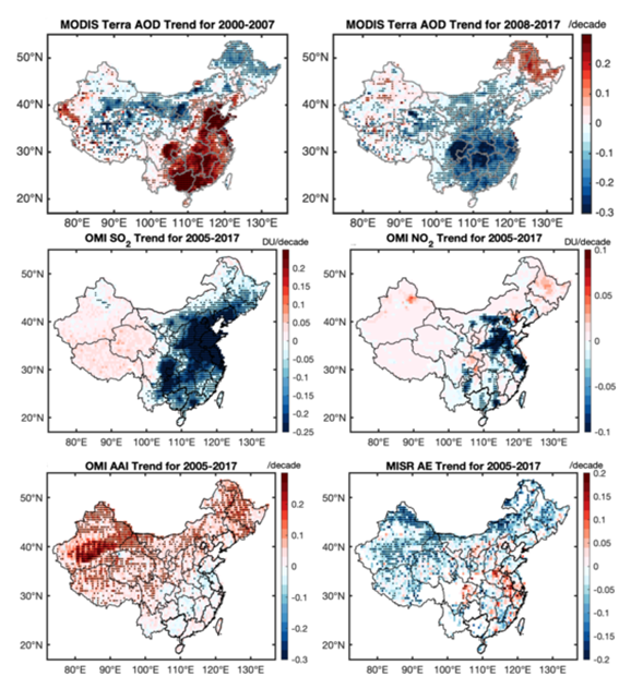
:Satellite sensors can provide unique views of global pollution information from space. In particular, a series of aerosol and trace gas monitoring instruments have been operating for more than a decade, providing the opportunity to analyze temporal trends of major pollutants on a large scale. In this study, we integrate aerosol products from MODIS (MODIS Resolution Imaging Spectroradiometer, all abbreviations and their definitions are listed alphabetically in Abbreviations) and MISR (Multi-angle Imaging Spectroradiometer), the AAI (Absorbing Aerosol Index) product from OMI (Ozone Monitoring Instrument), column SO2 and NO2 concentrations from OMI, and tropospheric column ozone concentration from OMI/MLS (Microwave Limb Sounder) to study temporal changes in major pollutants over China. MODIS and MISR consistently revealed that column AOD (Aerosol Optical Depth) increased from 2000, peaked around 2007, and started to decline afterward, except for northwest and northeast China, where a continuous upward trend was found. Extensive negative trends in both SO2 and NO2 have also been found over major pollution source regions since ~2005. On the other hand, the OMI AAI exhibited significant increases over north China, especially the northeast and northwest regions. These places also have a decreased Angstrom exponent as revealed by MISR, indicating an increased fraction of large particles. In general, summer had the largest AOD, SO2, and NO2 trends, whereas AAI trends were strongest for autumn and winter. A multi-regression analysis showed that much of the AOD variance over major pollution source regions could be explained by SO2, NO2, and AAI combined, and that the SO2 and NO2 reduction was likely to be responsible for the negative AOD trends, while the AOD increase over NE and NW China may be associated with an increase of coarse particles revealed by increased AAI and decreased AE. In contrast to aerosols, tropospheric ozone exhibited a steady increase from 2005 throughout China. This indicates that although the recent emission control effectively reduced aerosol pollutants, ozone remains a challenging issue and may dominate future air pollution.

1. Introduction
In recent years, China has been facing a challenging air pollution problem in the background of its rapid industrialization and economic development. Especially in the past two decades, the frequent occurrence of haze and smog days has brought about considerable damage to both the environment and human health [1] as well as perturbations to the climate [2]. As a result, pollution in China has become the focus of many studies in China and worldwide. The major emission source of anthropogenic pollutants in China is fossil fuel burning, especially coal burning [3,4]. Studies have shown that this source has contributed to over 80% of SO2 pollution in China [5]. In urban areas, traffic is also an important source that greatly contributes to NOx, ozone, and particulate matter pollution [3,6,7]. In the winter, north China typically suffers from increased black carbon emissions from heating [8,9]. Seasonal biomass burning [10] and dust storms [11] also impair air quality over north and southeast China. Transboundary transport is another factor that impacts on air quality in China. For example, studies have shown that the trans-Eurasian transport of air pollutants can significantly contribute to surface ozone concentration in west China [12], whereas south China can be affected by pollution transported from South Asia [13] and Southeast Asia [14,15,16]. To combat air pollution, the Chinese government has enforced a series of emission control policies in the last few years to reduce the emission of major pollutants such as sulfur dioxides and carbonaceous aerosols [17]. Analysis using satellite datasets has indicated the effectiveness of these policies, with remarkable reductions in NOx [18,19,20], SO2 [21], or particulate matter [22]. These studies also prove that satellite measurements effectively reflect the spatial-temporal changes of the pollution condition and can be used for investigating long term trends.
Nonetheless, most of the previous studies only relied on a single dataset (e.g., AOD from MODIS or NO2 from OMI). There is still a lack of an integrated analysis using retrievals from multiple sensors that are available, which is likely to produce more complete and robust results. On one hand, different measurements of the same parameter such as AOD from MODIS and MISR, can cross-validate each other to achieve a more reliable result. On the other hand, analyzing the retrieval of multiple species can offer insights into the compositional changes of the pollution. For example, trends of SO2 and NO2 imply changes of sulfate and nitrate aerosols, whereas trends of carbonaceous and dust aerosols can be inferred from the AAI [23] and the AE (Angstrom Exponent). Moreover, although changes in aerosols and related trace gases have been extensively studied using satellite datasets, less attention has been paid to another major pollutant: tropospheric ozone. Given its complicated sources and formation mechanism, the control of ozone pollution is even more difficult than that of particulate matter. It has been implied that ozone will likely become the dominant pollutant in China in the near future [24,25].
To address the above-mentioned shortcomings, this study used aerosol and trace gas retrieval products from multiple satellite sensors to comprehensively investigate the temporal trends of major pollutants in China including aerosols, SO2, NO2, and tropospheric ozone for the past ~15 years. The relationships of SO2, NO2, AAI, and AE with AOD were also examined to explain the possible compositional changes of aerosols. This study can contribute to our understanding of regional pollution changes and the effectiveness of control measures, and serve as a reference for future environmental and climate modeling works.
The rest of this paper is organized as follows. Section 2 describes the multi-sensor data used in the study. The analysis method is described in Section 3. Pollution trends from multiple satellite datasets are presented in Section 4, and the conclusion with a brief discussion is given in the final section.
2. Materials and Methods
2.1. Datasets
2.1.1. MODIS and MISR Aerosol Optical Depth and Angstrom Exponent
The MODIS instrument is a single-view imager with a swath width of 2330 km and near global coverage every two days. This high sampling frequency captures most of the aerosol variability and microphysics properties. MODIS was launched on EOS Terra in 1999 and on EOS Aqua in 2002. We used Collection 6.1 Level 2 AOD products [26,27] from both of these platforms. The variable used was the quality controlled dark target and deep blue combined AOD at 550 nm over land, and the time period spanned from 2000 to 2017. The land AOD product uncertainty was estimated to be 0.05 ± 20%AERONET (Aerosol Robotic Network) AOD. Only QC = 3 data were selected to ensure data quality. We gridded the pixel level data into daily means at 0.5° × 0.5° resolution, and only grids with more than half the available pixel level data were considered valid. To calculate the monthly means, we applied two schemes, namely threshold equal day averaging and pixel weighted averaging, as Levy et al. [28] indicated that substantial differences in the monthly means could be caused by different averaging schemes. The two schemes were found to have a negligible impact on the trend (figure not shown). We thus only show the results using 5-day threshold equal day averaging (i.e., each month must have at least five valid daily means).
MISR is a multi-angle sensor with nine pushbroom cameras on the EOS Terra platform. The zonal overlap of the common swath of all nine cameras is at least 360 km in order to provide multi-angle coverage in nine days at the equator, and two days at the poles [29]. Compared to MODIS, the multi-angle view of MISR performs better over bright surfaces, while its lower sampling may not fully resolve small-scale variability. In addition to AOD, the AE is also a useful parameter indicating the composition of fine/coarse particles. Therefore, we used version 31 Level 3 gridded monthly mean AOD and AE products [30,31,32] with a 0.5° resolution from 2000 to 2017. The reported MISR AOD uncertainty is 0.05 or 20%AOD [33,34]. Note that MODIS AE over land is considered unsuitable for quantitative research [13] and we thus only used those data from MISR.
2.1.2. OMI Absorbing Aerosol Index
The OMI launched onboard the EOS Aura in 2004 [35] provides an absorbing aerosol index (AAI) product, which constituted a qualitative indicator of the presence of UV absorbing aerosols in the atmosphere such as biomass burning and dust [36]. The AAI calculations were based on the difference in surface reflectivity derived from the 331.2 and 360 nm backscatter radiance, exhibiting an uncertainty of ±30% [36]. The AAI dataset used in this study was the version 3 Level 2 daily product with 0.25° resolution from the near UV algorithm [37,38] during the 2005–2017 period. As clouds and scattering aerosols can also produce small positive AAI, we only retained AAI values greater than 0.7 to represent absorbing aerosols as suggested by Prospero et al. (2002) [39]. Then, the monthly means were calculated with a 5-day minimum threshold. Although more quantitative products such as the absorption aerosol optical depth and single scattering albedo are also provided, these data tend to have greater uncertainty arising from aerosol model assumptions in the retrieval algorithm. Therefore, we used the AAI data here, which is the ratio of the directly observed radiance at two channels.
2.1.3. OMI SO2 and NO2
The measurements of SO2 and NO2 are also explicit objectives of OMI. We used the operational OMI planetary boundary layer SO2 product processed with the improved band residual difference algorithm [40,41,42]. The algorithm uses differential residuals at the three wavelength pairs with the largest differential SO2 cross sections in the OMI UV2 spectral region (310–380 nm) to maximize measurement sensitivity to anthropogenic emissions in the PBL (Planetary Boundary Layer). Validation against field measurements indicates accuracy of ~1.5 DU (Dobson units) over East China [43].
The tropospheric column NO2 data used are from the NASA standard product version 3 [41]. It uses the new algorithm described in [43]. The average error reported in the data file was 2.2 × 10¹⁵ molecules/cm2. For consistency with SO2, the data were converted from molecules/cm2 to Dobson unit (1 DU = 2.69 × 10¹⁶ molecules/cm2).
The original product used was version 3, Level 3 daily mean SO2 and NO2 products with 0.25° resolution [38]. The data were further gridded into monthly means at 0.5° × 0.5° resolution, for the purpose of multi-regression analysis. The study period was also from 2005 to 2017.
2.1.4. OMI/MLS Tropospheric Ozone
As OMI only retrieves the total column ozone, a joint algorithm was developed to retrieve the tropospheric ozone with the MLS also onboard Aura [44]. The OMI ozone data were provided on a 1° × 1.25° grid for each day. There are typically 3494 MLS Level 2 Version 1.5 along track profile per day over the globe with horizontal resolution of 150 km and vertical resolution of 3 km in the upper troposphere and lower stratosphere. OMI is matched with each MLS profile by linearly interpolating the nearest four 1° × 1.25° grids. Then, the corresponding MLS ozone profile was integrated from the tropopause to the top of the atmosphere and extracted from the matched OMI total column ozone. The final tropospheric ozone data was gridded with 1° × 1.25° grid for each month [45]. The OMI/MLS tropospheric ozone data compared well with ozonesondes and chemical transport models [46,47] in terms of large scale features including the mean value, seasonal cycle, and zonal variations, although over high latitudes and the Sahara desert, a larger different exceeding 5 DU can be observed.
2.2. Methods
2.2.1. Trend Estimation
The linear trends are estimated using the monthly mean data with the Sen’s slope method [48]. This is a non-parametric estimation and is less sensitive to outliers compared to linear regression. The Sen’s slop is defined as the median of the slopes of all data pairs:
where b is the Sen’s slope and Xi and Xj are the ith and jth data in the time series, respectively.
To test the significance of the trend, we used the Mann–Kendall statistical test [49,50]. This is also a nonparametric test to identify the existence of monotonic trends in a time series. The MK test statistic is calculated as:
where
which follows a normal distribution with zero mean and variance.
Moreover, studies have found that the existence of serial correlation in the time series will increase the probability that the MK test detects a significant trend [51,52,53]. We thus pre-whitened the time series to remove serial correlation following the procedure recommended by [53]. Specifically, the linear trend is first removed from the time series using the Sen’s slope b:
Then the AR(1) process is estimated and removed:
where is the lag−1 autocorrelation, and finally the linear trend is added back:
2.2.2. Multiple Regression
To investigate the relationship between AOD and the components (AAI, SO2, and NO2 as precursors for sulfate and nitrate aerosols respectively), we performed a multiple regression analysis as:
The time series for AOD, AAI, SO2, and NO2 are first de-seasonalized and de-trended, by removing the multi-year averaged seasonal cycle and linear trends, respectively, and then normalized by their respective standard deviation. In this way, the magnitude of each regression coefficient can reflect the relative contribution of the corresponding variable to the total variance of AOD. The significance of the model as well as each coefficient is tested using the F test. In addition, because significant correlation may exist between some species such as SO2 and NO2, which will impact on the accuracy of the multi-regression coefficients [54,55], we also performed a single parameter regression of AOD against each species to verify the credibility of the coefficients.
3. Results
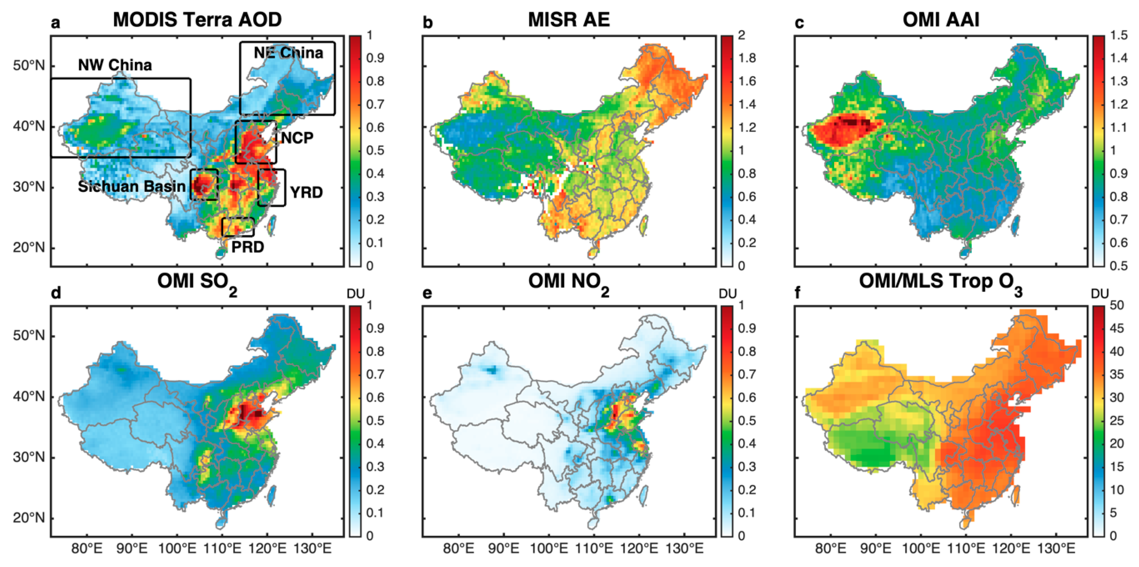
Before discussing the trends, we first briefly examine the spatial distribution of the parameters used in this study (Figure 1). It was seen that the highest AOD values (up to 1) mainly concentrated on East China and the Sichuan Basin, corresponding to the most densely populated areas. NW China’s Taklimakan Desert also showed some high AOD signals, resulting from wind-blown dust. East China also had the highest SO2 and NO2 concentrations, especially the NCP (North China Plain) region. AE exhibited higher values over East China than the west, and the lowest values were found in the Taklimakan Desert. This is also consistent with the general aerosol size distribution as East China is dominated by fine anthropogenic aerosols whereas dust is typically found over the desert region in the west. The spatial distribution of AAI also showed a hotspot in the Taklimakan Desert, with some moderately high values found over the NCP and NE China. The former is the result of dust aerosols, while the latter should be mainly attributed to carbonaceous aerosols considering the higher AE values there. The spatial distribution of tropospheric O3 was more spatially uniform than the aerosol and the other two gas components, and largely follows the topography (i.e., higher concentrations over low altitudes and lowest concentration over the Tibetan Plateau). In general, the parameters examined reflect the spatial distribution of major pollutants in China.
3.1. AOD Trends
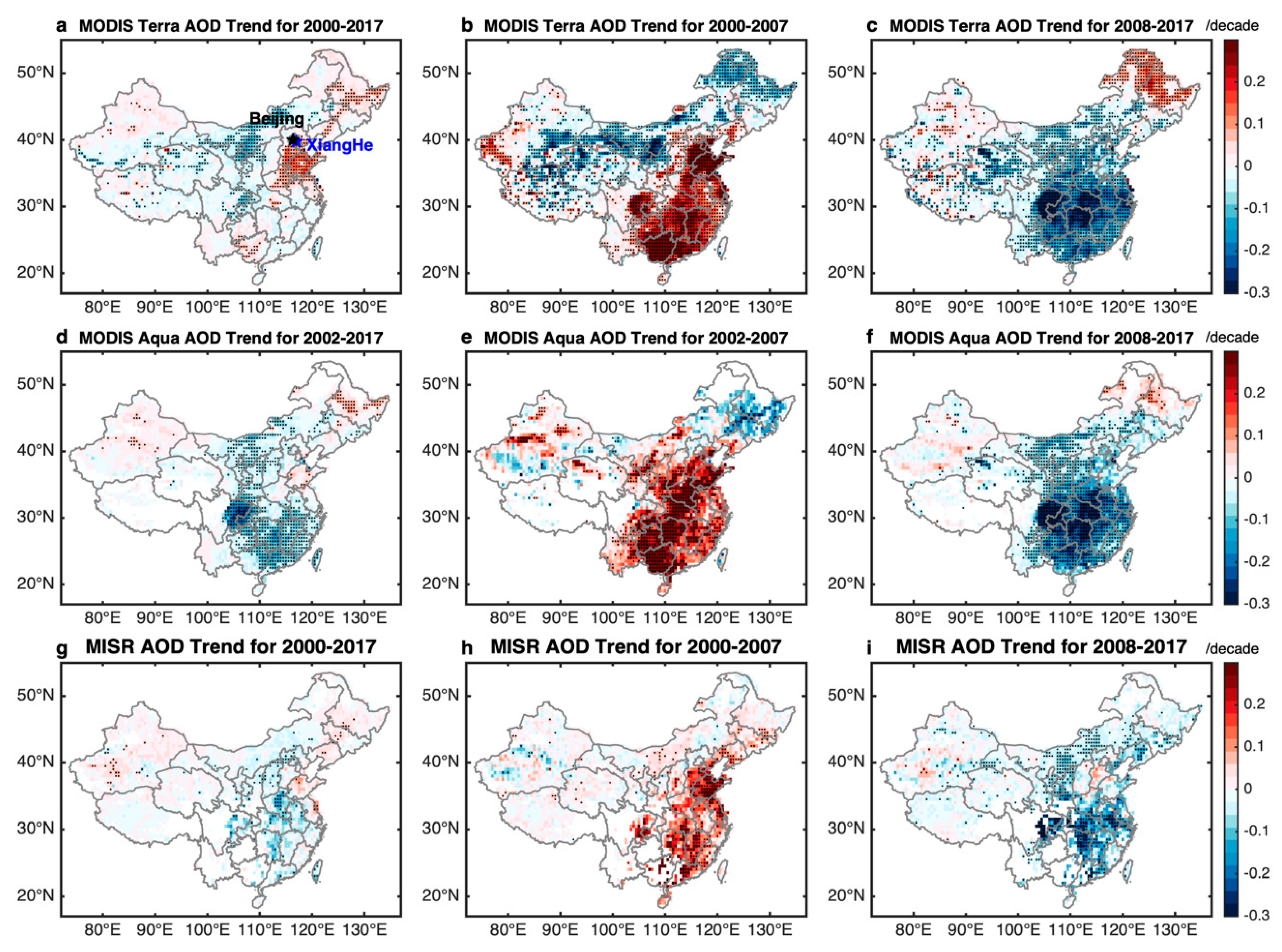
The linear trends for MODIS and MISR AOD are shown in Figure 2. During the whole period of 2000 to 2017, the MODIS Terra data indicated weak increasing trends over the NCP and NE China and weak decreasing trends over Inner Mongolia to the northwest of the NCP (Figure 2a), MODIS Aqua exhibited significant negative trends over South China and insignificant positive trends over NE China (Figure 2d), while MISR showed weak significant negative trends in parts of South China, but largely insignificant trends elsewhere (Figure 2g). Through closer examination, we found that there appeared to be a sharp trend change in 2008. Before 2008, both MODIS and MISR data showed strong and significant positive changes as large as 0.3/decade over the entire East China (middle column). After 2008, in contrast, prevailing negative trends with comparable magnitudes were found over China (right column). The only exception is in NE and NW China, where positive trends were noticed. This trend shift around 2008 was also previously noticed by [56] using MODIS data.
To corroborate satellite retrieval products, we also examined the trends at two ground sites within the AERONET, which is a surface network of high quality sunphotometer measurements of aerosol properties, whose data are often used to validate satellite retrievals [57]. The two sites were Beijing and XiangHe, which are both located in the NCP and are the only two sites with sufficiently long data records for long term trend estimation. From Figure 3, it is clearly seen that both these sites exhibited trend shifts from positive to negative around 2008, which is consistent with the satellite data.
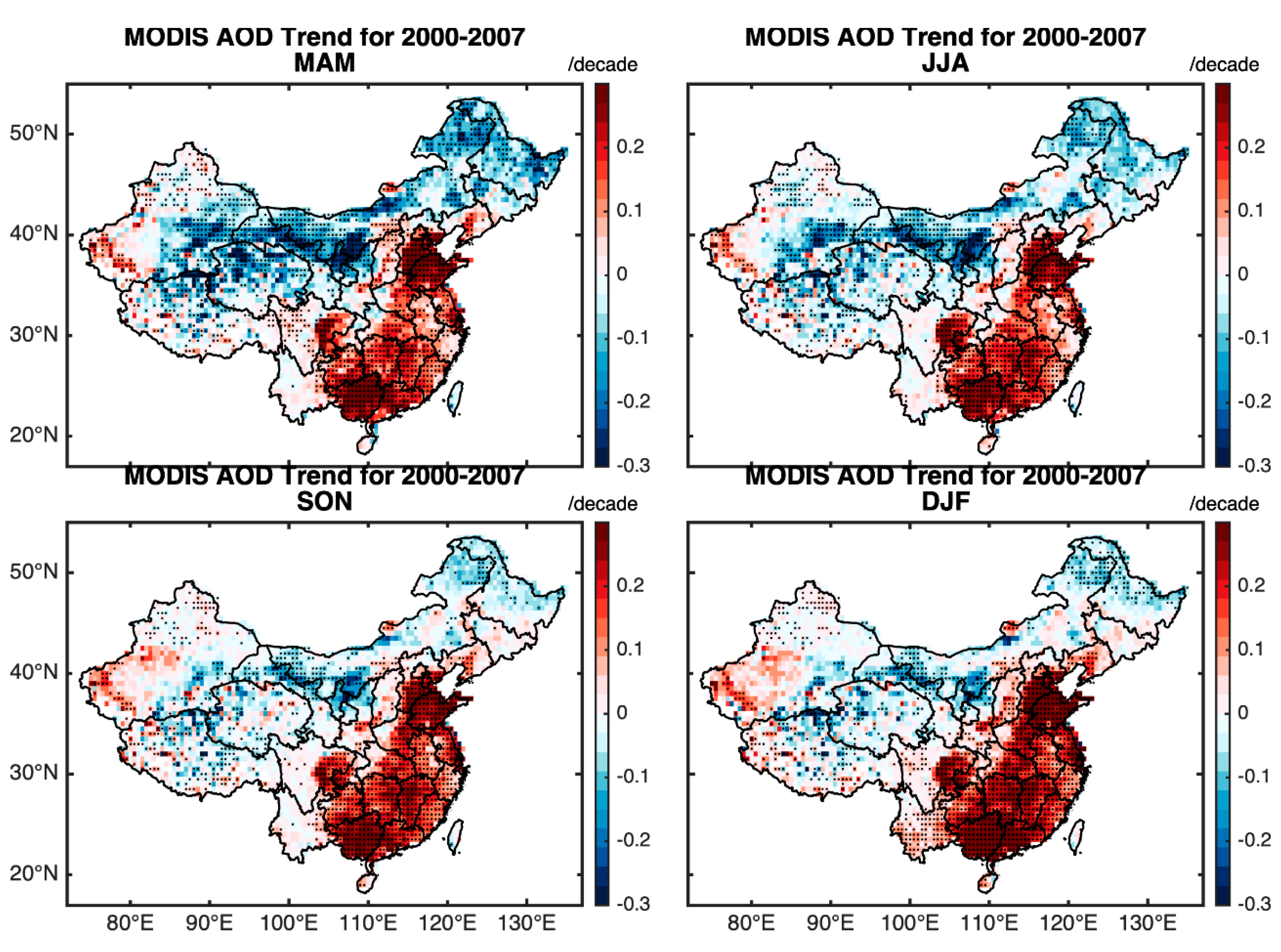
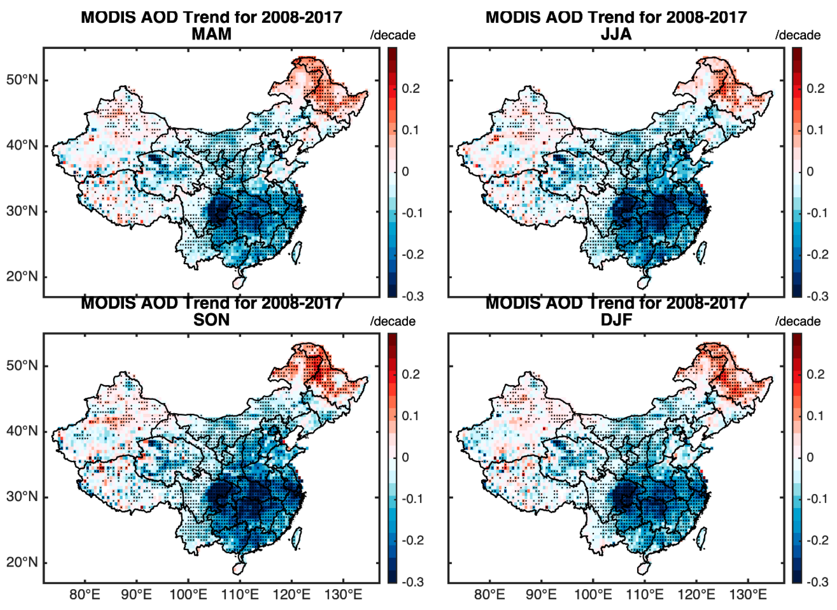
The seasonal AOD trends from MODIS showed a very similar pattern to the annual trends (Figure 4 and Figure 5) and little differences were found between the results of the four seasons. To save space, only the MODIS Terra results are presented here because the Aqua results were quite similar. In general, before 2008, the winter (DJF, December, January, February) showed the strongest increase, especially over the NCP and PRD, where the trends exceeded 0.3/decade, whereas the trend during the other seasons was generally between 0.1–0.2/decade. After 2008, the summer (JJA, June, July, August) and fall (SON, September, October, November) trends appeared slightly stronger, especially for the southern part. Note that we did not use MISR for seasonal analysis, mainly because we observed more variability and missing data in the MISR time series, probably related to its lower sampling frequency than MODIS. This sampling difference may also explain many of the trend differences between MODIS and MISR in Figure 2.
3.2. AAI and AE Trends
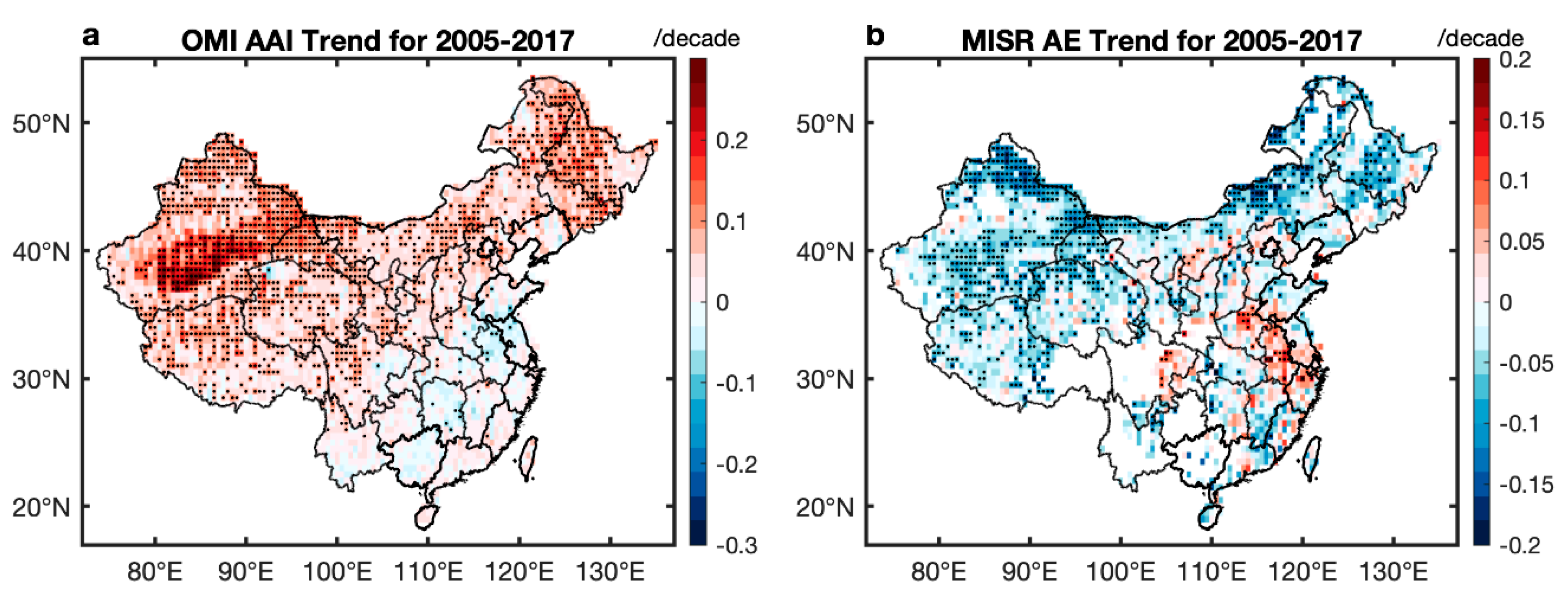
The AAI is defined as the difference between the ratio of two satellite observed radiances at the UV channel and those calculated for a pure Rayleigh atmosphere. It is a measure of the wavelength-dependent reduction of Rayleigh scattered radiance by aerosol absorption. By theory, it is related to the amount and height of UV absorbing aerosols [23] including dust, black, and organic carbon. Therefore, it offers insights into aerosol composition. Figure 6a shows the annual trends of OMI AAI during the 2005 to 2017 period (the trends from 2008 to 2017 are similar). Significant increases were noted over most of North China. The strongest positive trends were found in the Taklimakan Desert in the Xinjiang Province of NW China. The trends there reached ~0.27/decade, while over the other regions with positive trends, the trend amplitude was mostly below 0.2/decade. For the southern part where significant negative AOD trends were observed during this period, the AAI trend was weak and insignificant.
Since the AAI increases can be caused by changes in the loading of either dust or carbonaceous aerosols or both, we also examined the trend for MISR AE (Figure 6b). The AE is related to particle size and a lower AE indicates larger sizes in general. Comparing Figure 6a and Figure 6b, it can be clearly seen that the regions with positive AAI changes corresponded well to those with negative AE trends. This suggests an increase in the mean particle size, which is mostly likely due to increased dust fraction. Considering that NW China is also a major dust source region, increased dust activity can well explain the observed AAI and AE trends. The trends in NE China might be associated with increased dust transport from the west.
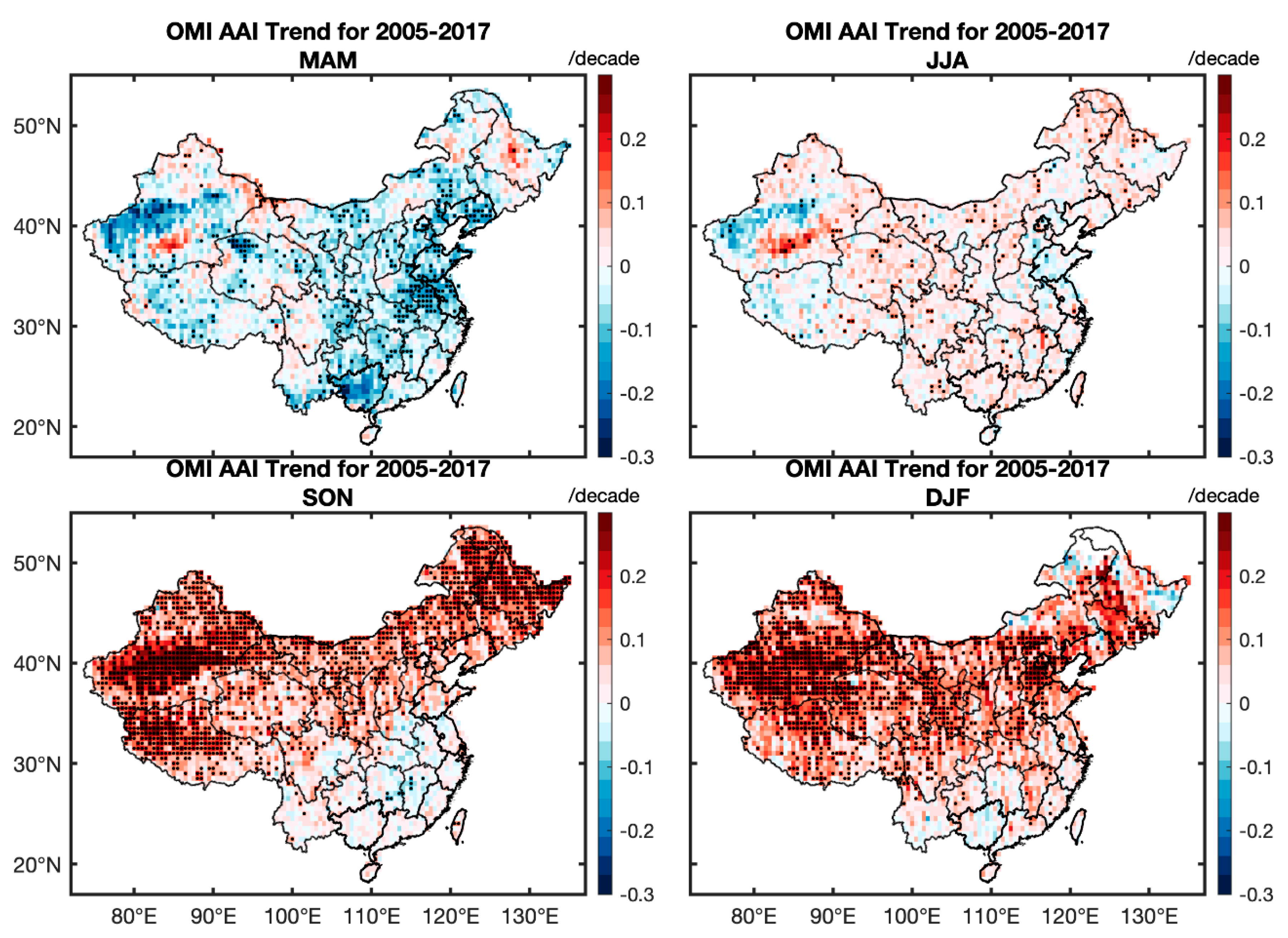
Seasonally, the strongest AAI increase happened in the fall and winter (Figure 7). This is somewhat inconsistent with the dust outburst season, which is usually in the spring. However, precious studies have also indicated increased dust emission in the late fall–winter season [58,59]. We also noticed the strongest negative trends in MISR AE for SON (figure not shown), while for winter, the MISR data availability was too low to estimate significant trends.
Relating the AAI trends to those of AOD, it was noticed that the regions with an AAI increase largely corresponded to regions with positive AOD trends during the 2008–2017 period (i.e., NE and NW China, as seen in Figure 2c). The seasonality was also in phase with the most notable changes in the fall and winter, although the AOD trends appeared weaker. This makes sense since dust only accounts for a small fraction of total aerosols in these two seasons. Moreover, since AAI is not linearly related to dust concentration, its change cannot reflect the absolute change in the dust amount.
It is worth noting that AAI is a qualitative indicator of absorbing aerosols and its trends should be interpreted with caution. According to previous studies [34,60,61], apart from the column loading of absorbing aerosols, AAI is also sensitive to absorbing aerosol layer height, surface albedo, clouds, and ozone concentration. We then discuss the possible impact of these four factors on the observed trends in detail. First, the aerosol layer height is typically highly correlated with PBLH (Planetary Boundary Layer), and previous studies have indicated that AAI is positively related to the PBLH. However, Guo et al. (2019) [62] revealed a downward PBLH trend over China since 2004, which means that the change of BLH would cause a decreasing AAI trend, opposite to what we have shown. Next, the increase of surface albedo has two competing effects on AAI: a higher albedo may enhance aerosol absorption and thus increase AAI, while also increasing the total amount of reflected radiation at the top of the atmosphere, which may reduce the AAI. De Graaf et al. (2005) [60] indicated that the overall effect will be dominated by the first mechanism (i.e., increasing surface albedo may increase AAI). Although a long-term surface albedo dataset is not readily available, a recent study by Chen et al. (2019) [63] found that the leaf area of vegetation has significantly increased over China since 2000 by using satellite measurements. This suggests that surface albedo is likely to be decreased during this period as vegetation has a lower albedo than bare lands. This decreased surface albedo would lead to a decreased AAI trend, which is again in contrast to the observation. Third, the effect of clouds on AAI is more complicated and depends on the relative height of the cloud and aerosol layer. The accurate analysis of this effect requires long term observations of the collocated cloud height and aerosol height, which is rather difficult to obtain. Nonetheless, Li et al. (2018) [64] found that cloud fraction over China did not exhibit significant trends, therefore, we consider that the change of clouds is unlikely to be a dominant factor for the AAI change. Finally, absorption of ozone in the UV range will also increase the AAI value. The AAI product already increased the correction of ozone absorption. For the study period, although we noticed an increase in tropospheric ozone over China (Section 3.5), ozone absorption was dominated by stratospheric ozone and the change in tropospheric ozone was only a minor contribution to total ozone absorption. Moreover, the spatial distribution of the ozone trends was not consistent with the AAI trends. These facts suggest that ozone change is also unlikely to be responsible for the AAI trends. In sum, factors other than absorbing aerosol loading that affect the AAI have mostly been ruled out. Combined with the negative AE trends, the positive AAI trends are thus mostly likely to be associated with increases in the amount of absorbing aerosols, especially dust.
3.3. SO2 and NO2 Trends
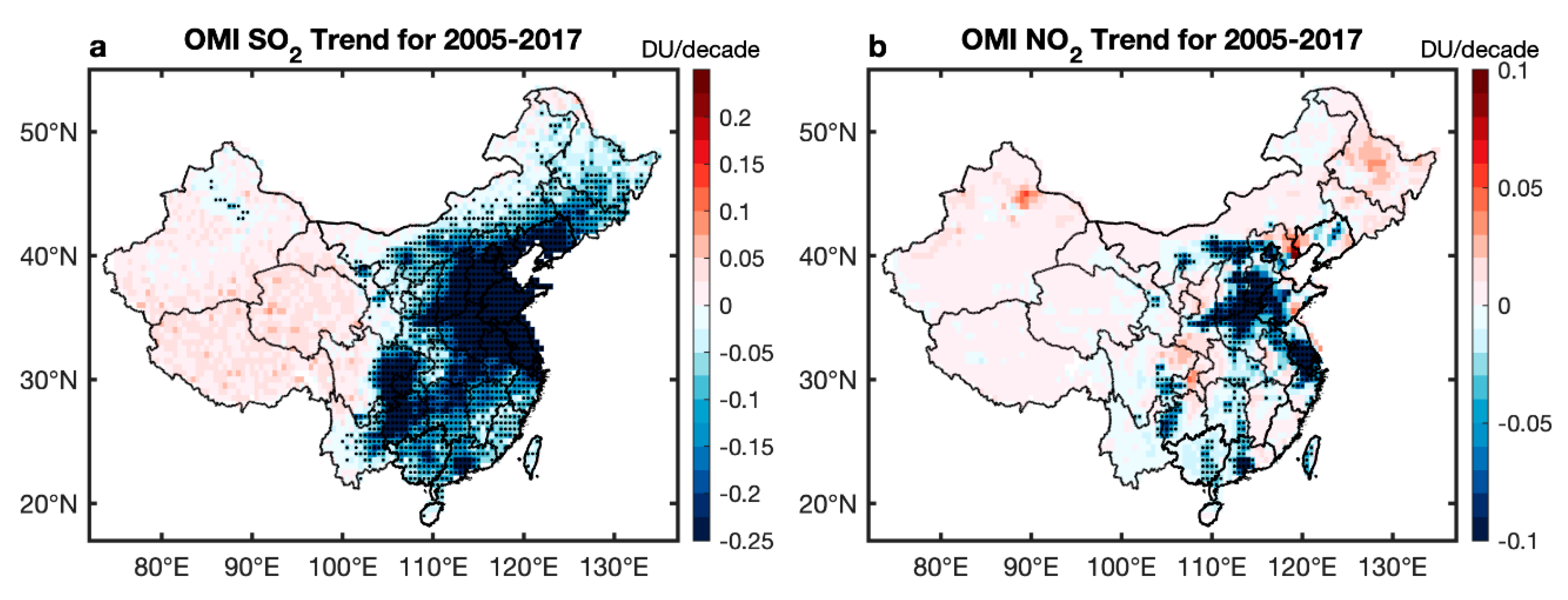
SO2 and NO2 are also major pollutants in China as well as precursors for sulfate and nitrate aerosols. Their trends directly reflect the emission changes, which may help explain the AOD trends. In Figure 8, we plot the annual trends for the column SO2 and NO2 concentrations retrieved by OMI for the 2005–2017 period. The spatial pattern of SO2 trends highly resembles that of AOD (Figure 2c,f,i), with significant decreases over East and South China, in particular, the major pollution source regions of the NCP, Sichuan Basin, and PRD. The distribution of trends for NO2 appears to be comparatively scattered and also exhibits significant negative trends over East China, but are mainly concentrated on the southern NCP, YRD, and the PRD. The major source of NO2 is automotive, so the highest emissions are typically found over densely polluted city conglomerates. Nonetheless, the SO2 and NO2 trends both indicate significantly decreased emissions of anthropogenic pollution and well agree with the negative trends of AOD for this time period.
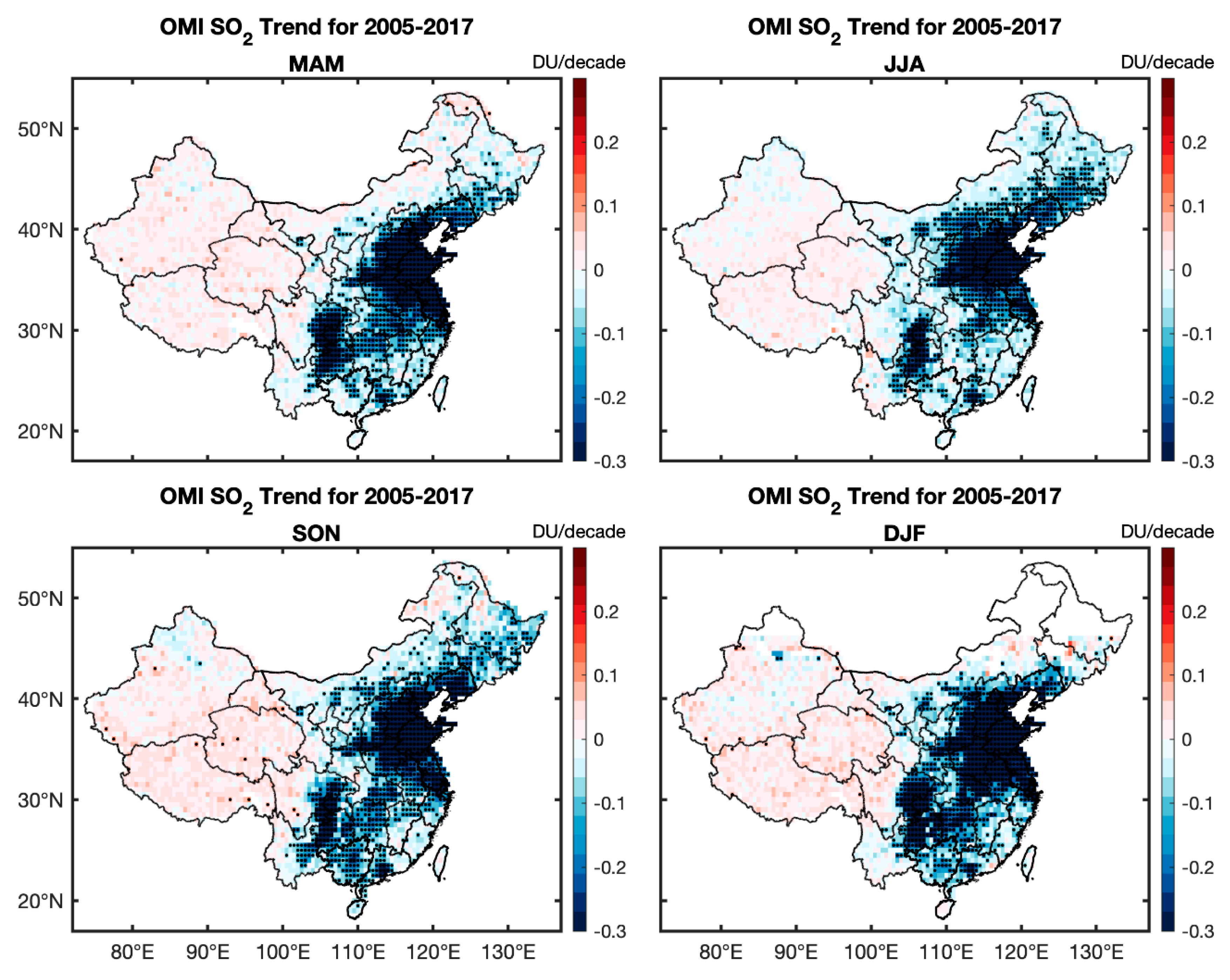
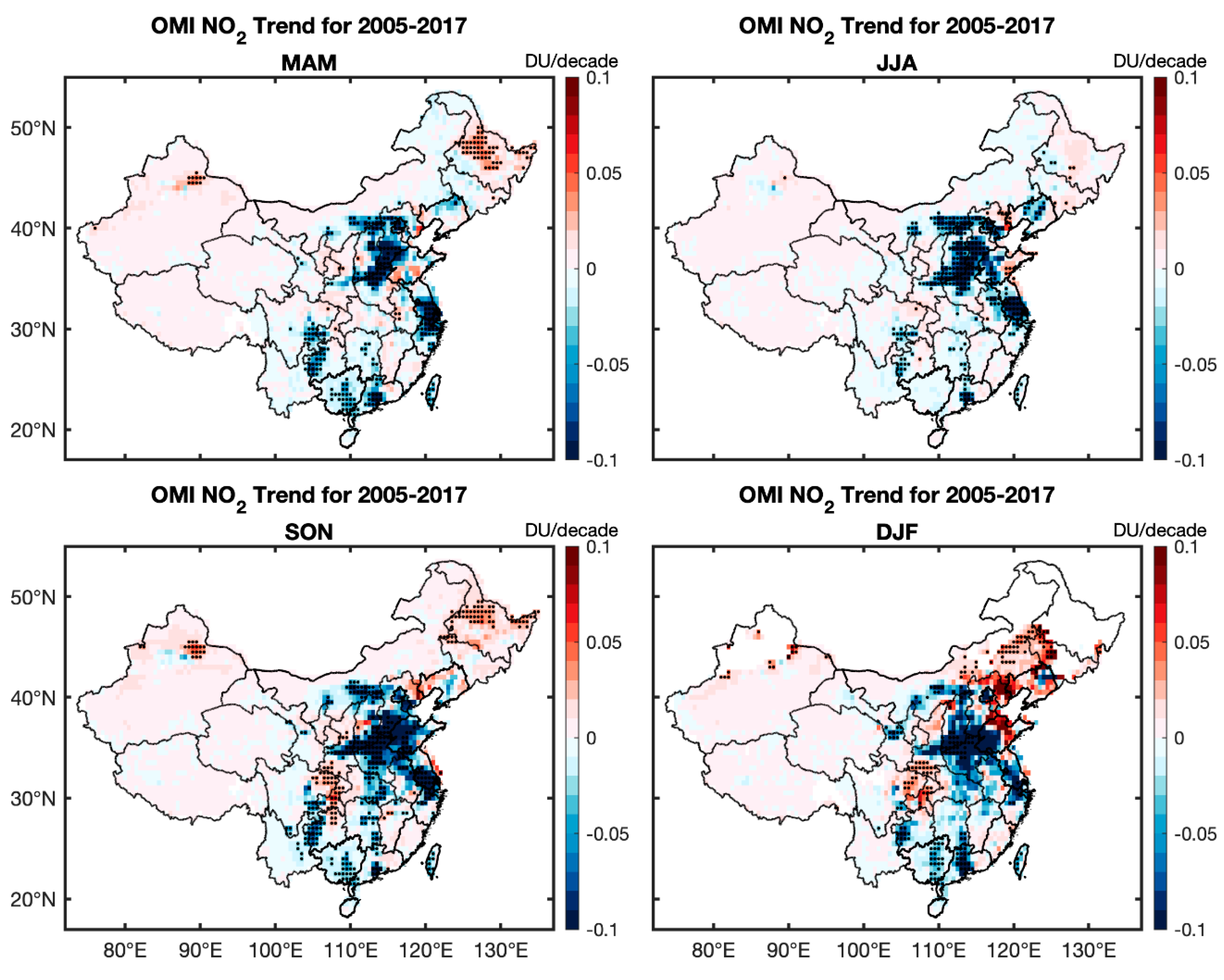
The SO2 trends for the four seasons were highly consistent with the annual trends (Figure 9). Regions with negative trends extended slightly to the northeast in the summer and fall. For seasonal NO2 trends, some differences were observed (Figure 10). Specifically, while overall, most areas over East China showed negative trends, during the winter and fall, significant increases were found in the northeast. This could also partly contribute to the increased AOD over NE China during these two seasons, in addition to dust.
The decreases of SO2 and NO2 are consistent with previous study by [65], who analyzed global trends of SO2 and NO2 from OMI, and are clear indications of the effectiveness of emission reduction measures taken in China during the past decade.
3.4. Multiple Regression
Multiple regression was performed on AOD against AAI, SO2, and NO2 according to Equation (7) to further investigate the possible compositional changes associated with the AOD trends. The variance of AOD explained by the multiple regression model, defined as the R2 value between the original AOD time series and the regressed time series, is shown in Figure 11. Note that the AOD variance here refers to the deviation from its multi-year averaged seasonal cycle. We notice that for the majority of places over North and East China, the regression model was significant and the variance explained reached 50% (corresponding to ~0.7 correlation) or higher. The highest variance explained was found over NW China’s Taklimakan Desert. This is not surprising because this region is dominated by dust aerosols, which is a primary aerosol species and can be well represented by the AAI. For most of the other regions, especially those in East China, the aerosol composition is more complex. Moreover, many aerosol species are secondary such as sulfate, nitrate, and organic aerosols, thus making the relationship between AOD and gas precursors ambiguous and variable. The regression model still performed well over major pollution source regions such as the NCP, PRD, YRD, and the Sichuan Basin. This is an indication of the success of the fitting, and that the decomposition of AOD variability into that of AAI, SO2, and NO2 is reasonable.
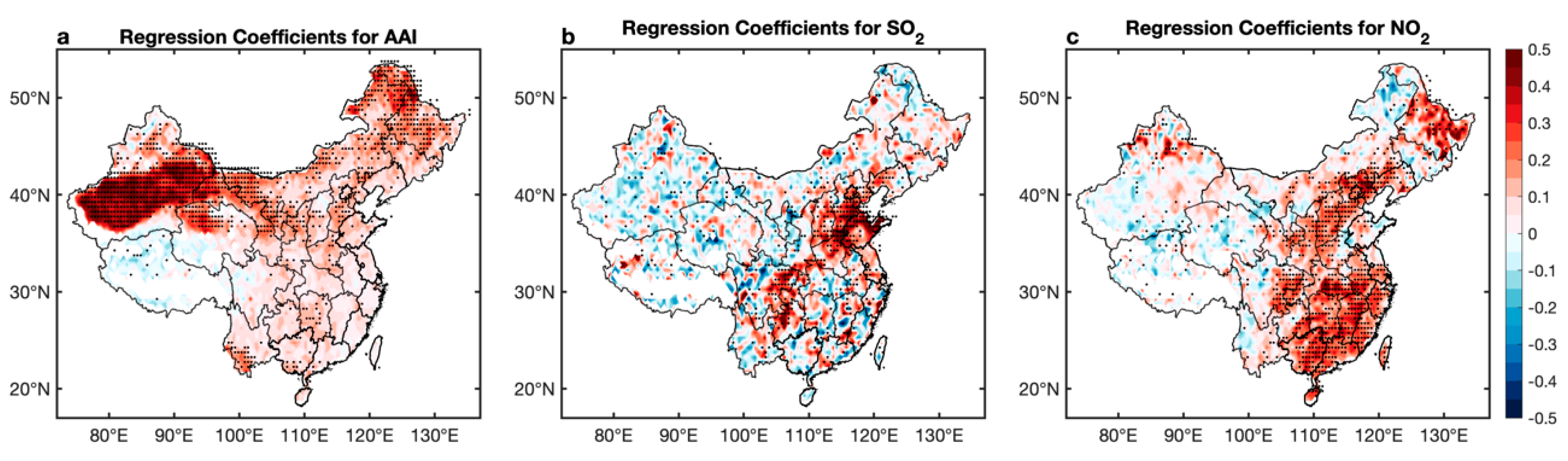
We continued to examine the regression coefficients as they reflect the relative contribution of each component to the total AOD given that all of the time series were normalized. Figure 12 shows the spatial distribution of the coefficients for AAI, SO2, and NO2. To examine the possible effect of multicollinearity on the accuracy of the regression coefficients, we compared the multi-regression coefficients with those obtained from the single parameter regression of AOD onto AAI, SO2, and NO2, respectively, and found that the magnitude and distribution of the coefficients were highly consistent (figure not shown). It can be clearly seen that the signals of AAI coefficients (Figure 12a) were mostly concentrated in the north, especially the desert area of the northwest, whereas the highest coefficients for SO2 (Figure 12b) and NO2 (Figure 12c) appeared in the east and the north. Again, this was expected, as dust is the major aerosol component in the northwest, thus high signals of AAI were found there. On the other hand, anthropogenic aerosols are the major contributor to AOD over East and South China, thus the AOD variability of the latter is more closely related to sulfate and nitrate precursors of SO2 and NO2, respectively. Note that even for SO2 and NO2, the distributions of the coefficients were not the same. The SO2 pattern showed two distinct centers over the NCP and the Sichuan Basin, respectively, with negligible signals elsewhere. For NO2, large positive coefficients were found over the entire East Asia and even the northeast, in particular, the coastal regions of Southeast and South China where the SO2 impact is low. Although SO2 and NO2 can both be produced by fossil fuel burning, they have different emission sources. SO2 is primarily released from coal burning while automobiles release the largest fraction of anthropogenic NO2. A large fraction of NO2 is also formed from natural processes such as lightning. The difference in the spatial distribution of SO2 and NO2 regression coefficients may reflect the different aerosol compositions in East and South China.
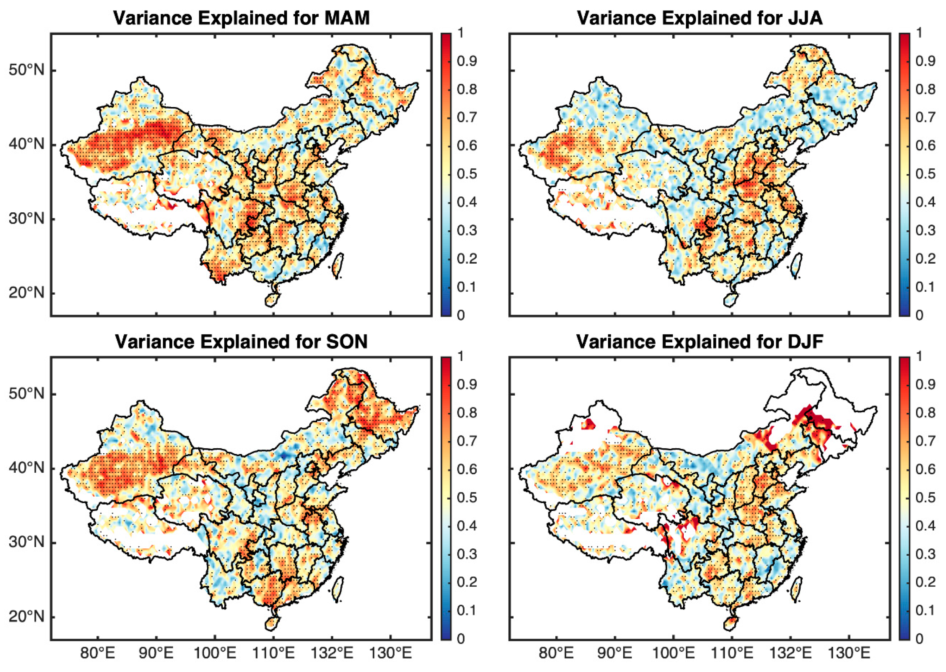
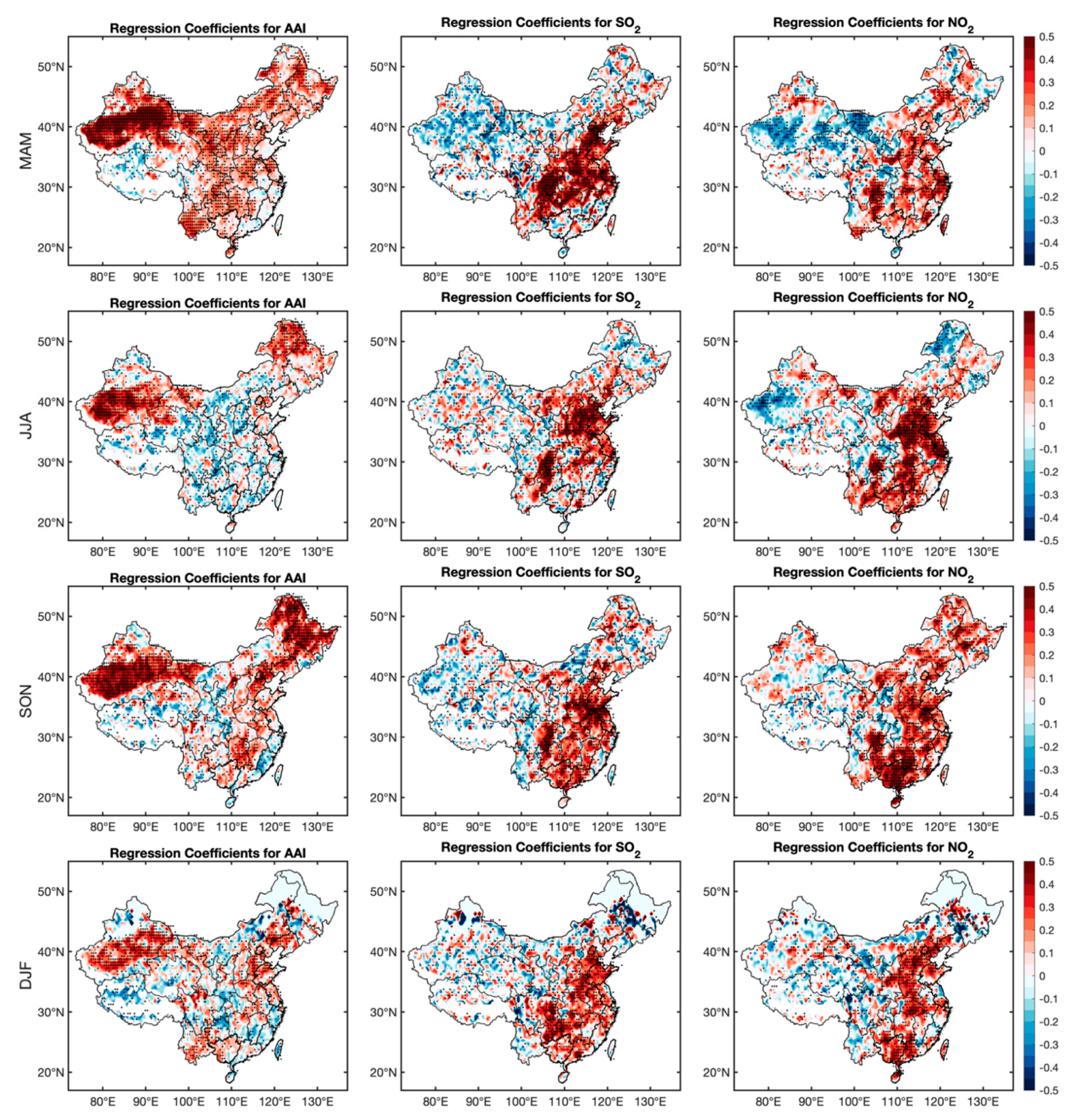
Seasonal multiple regression was also performed as the residence time and dominant pollution species tend to vary with season. The seasonal models also showed satisfactory fitting with the variance explained mostly over 50% (Figure 13). The spring season (MAM) had the best overall fitting. The missing values in winter (DJF) over the high latitudes and the Tibetan Plateau were due to the high surface albedo caused by the ice and snow surface. Figure 14 displays the seasonal regression coefficients for the three parameters. For the AAI, large positive signals exist over the Taklamakan Desert in all seasons. In the spring, positive signals extended over most of China, indicating wide spread dust events because this is the windiest season of the year. The positive signals can also extend to the NCP and parts of South China, except for summer (JJA). For the summer season, the concentrations of both dust and absorbing carbonaceous aerosols were in general lower than the other three seasons, which was due to decreased dust emission and increased scattering associated with the photochemical production of secondary species and higher aerosol water uptake. The regression coefficients of SO2 and NO2 showed less seasonality, both agreeing with annual results (Figure 12b,c) and concentrating over densely populated regions including the NCP, Southeast, and South China.
Overall, the multiple regression model using AAI, SO2, and NO2 as independent variables well fit the AOD variability and the spatial distribution of the coefficients was reasonable. Through this, combined with the AAI, SO2, and NO2 trends revealed previously, we can conclude that the decrease of AOD after ~2008 over East and South China is likely to be the result of reduced SO2 and NO2 emissions. Increase of dust (reflected by AAI) should be primarily responsible for the weak positive AOD trends over NW and NE China. However, caution should be taken in interpreting the multiple regression results, because (1) satellite retrievals bear certain sources of uncertainties, (2) the AAI, SO2, and NO2 are not directly related to the amount of dust, sulfate, and nitrate aerosols, and (3) like most statistical methods, correlation does not necessarily mean causality, and coincident measurements as well as modeling study is likely needed to confirm the causal relationship.
3.5. Tropospheric Ozone Trends
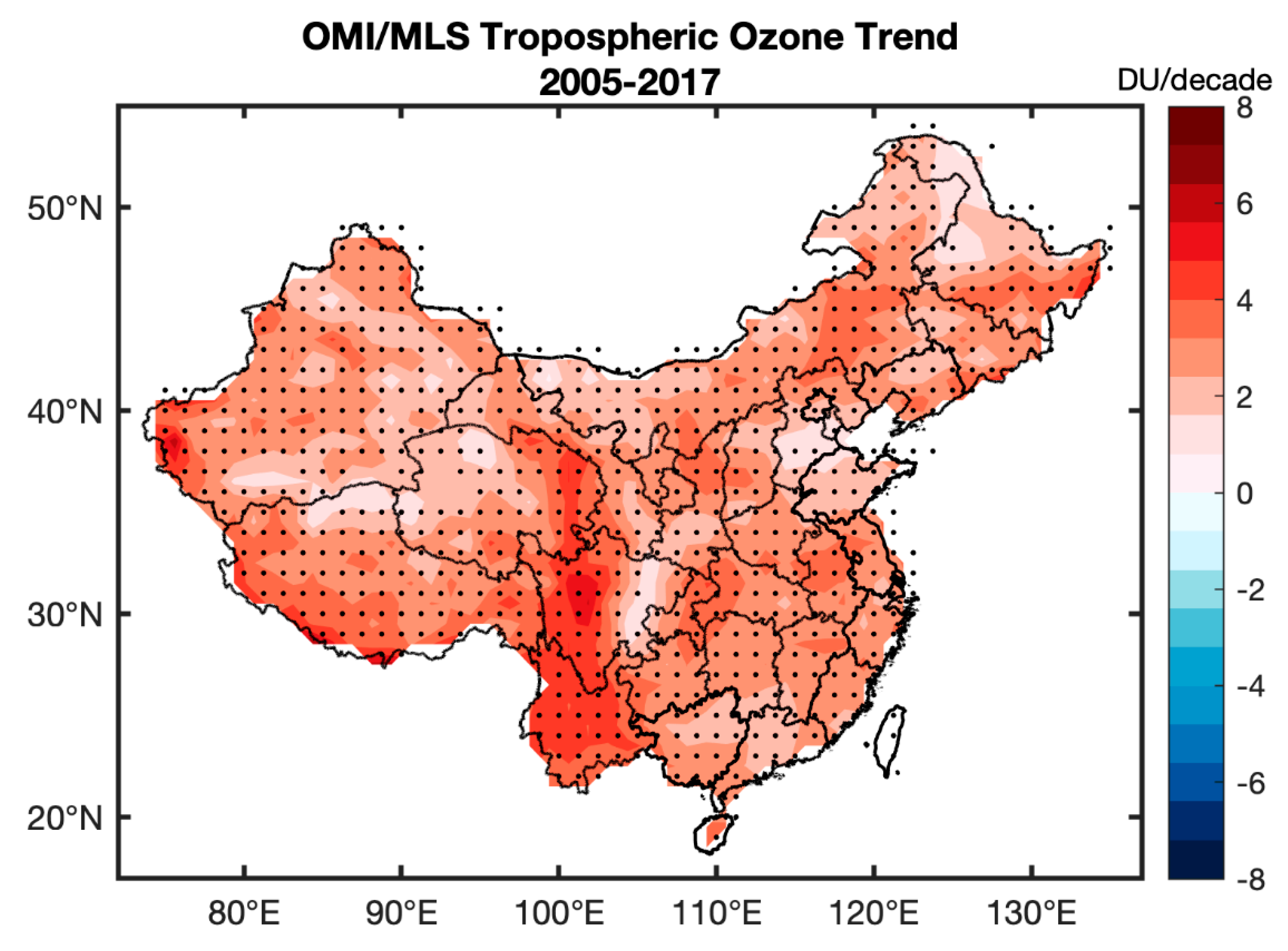
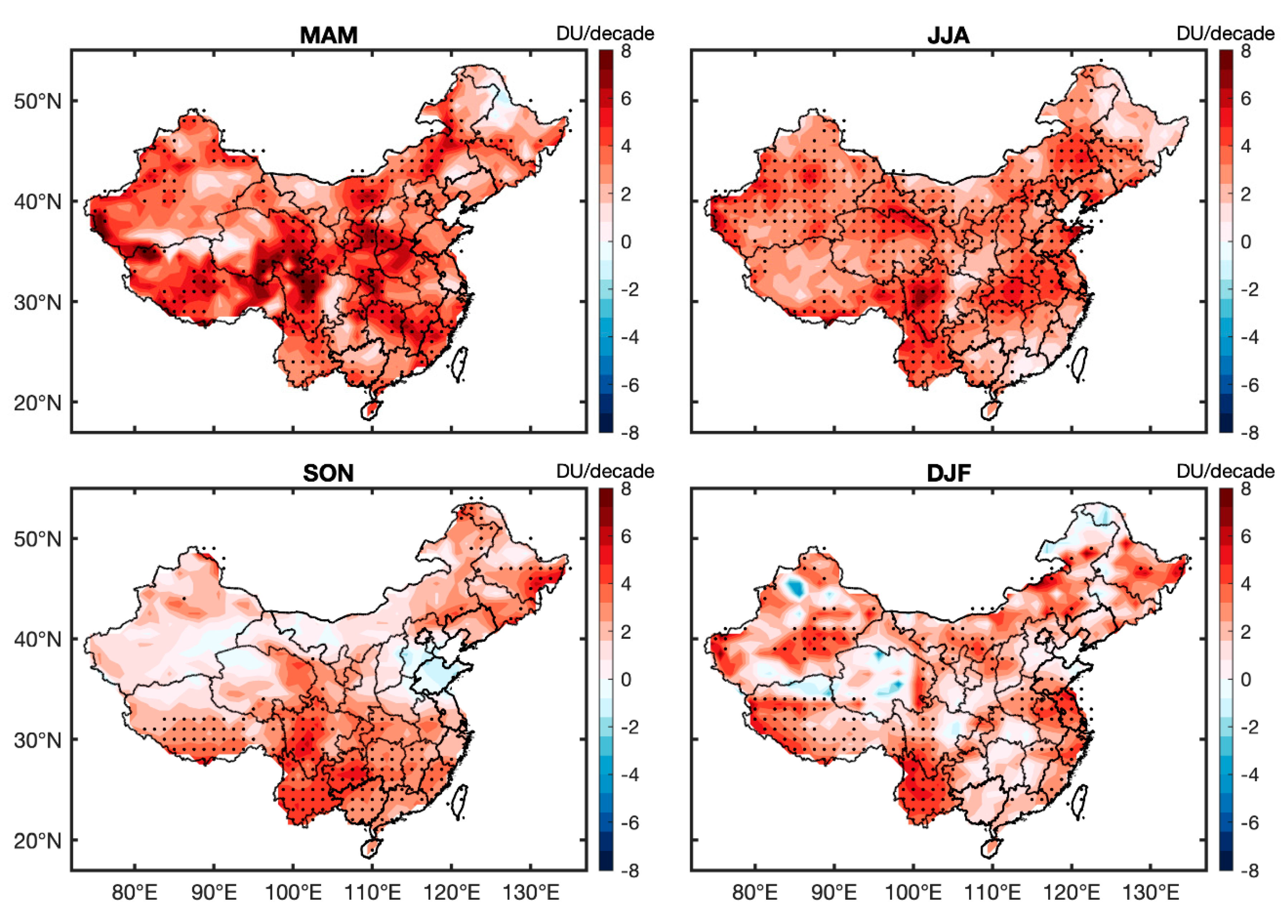
In contrast to aerosols, tropospheric ozone over China exhibits a nation-wide significant increasing trend on the order of 5 DU/decade (Figure 15). The spatial distribution of the trends is also much more uniform compared to aerosols, which is also consistent with the more uniform spatial distribution of tropospheric ozone (Figure 1). This should be reasonable considering the longer lifetime of ozone. The southwest region and edge of the Tibetan Plateau showed slightly higher trends, which is likely to be associated with transport from India and Southeast Asia [13,14,15,16,63] as the trends there appear stronger than in China (not shown in Figure 15). Distinct differences were observed in the seasonal trends (Figure 16). In general, spring trends were the strongest (5 DU/decade on average) while summer had the most significant trends (over 80% of the grids showed significant trends). The fall (SON) and winter (DJF) trends were mostly below 4 DU/decade and only ~40% of the grids showed significant trends. Tropospheric ozone pollution is typically heavier in spring and summer due to the high temperature and stronger surface solar radiation [66]. Therefore, it is natural that these two seasons exhibit greater changes than the other two seasons. This is most prominent for North China, whereas for a few regions including the Tibetan Plateau and Southwest China, larger increases were observed in the fall and winter.
The increase of tropospheric ozone in China has also been reported at scattered sites using ground observations [25,67,68]. Li et al. [69] further attributed this positive trend to the reduction of particular matter. Compared to ground observations, satellites have the advantage of revealing large scale patterns, and help to identify sources and transport features. The results shown here indicate that the worsening of ozone pollution is not local, but rather extends all over China.
3.6. Regional Trends
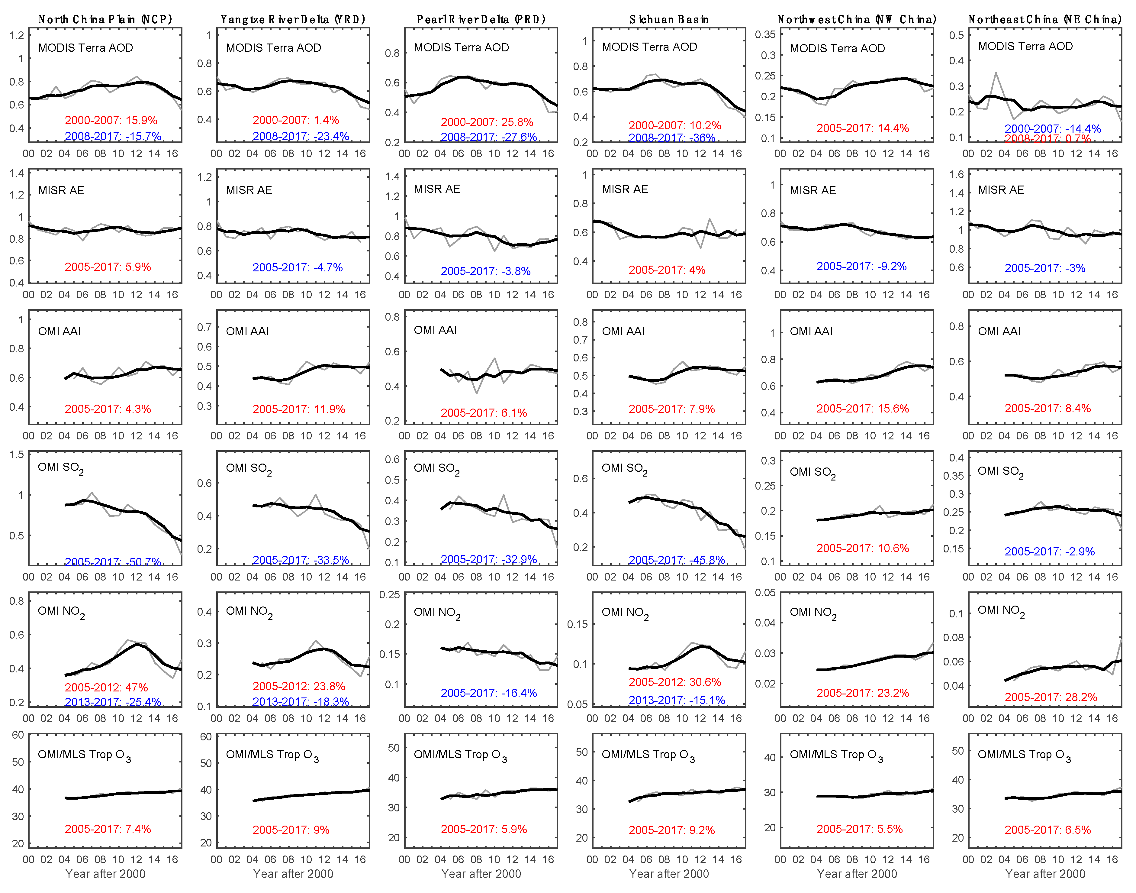
To better examine the variability of the pollutants as well as regional trend differences, in Figure 17, we plotted the annual time series of all pollutants over six representative regions marked on Figure 1a. The thick black lines in Figure 17 show the four-year moving average smoothed time series. The percentage of change is also marked on Figure 17 with positive changes shown in red and negative in blue.
The changes of the time series in Figure 17 can mostly be inferred from the trend maps shown previously, but some detailed regional features are still observed. For example, although in general, the AOD has started to decrease since 2008, at NCP, the AOD increased until ~2012 before a declining trend started. NO2 showed similar behaviors for the NCP, YRD, and Sichuan Basin, where it first increased until ~2012 and then experienced a sharp decline. Moreover, different to most of the country where overall negative AOD, NO2, and SO2 trends in the last decade were found, over NW China, these parameters were steadily increasing, together with AAI. This may be partly associated with the China western development strategy, which increased the emission of anthropogenic gases and aerosols.
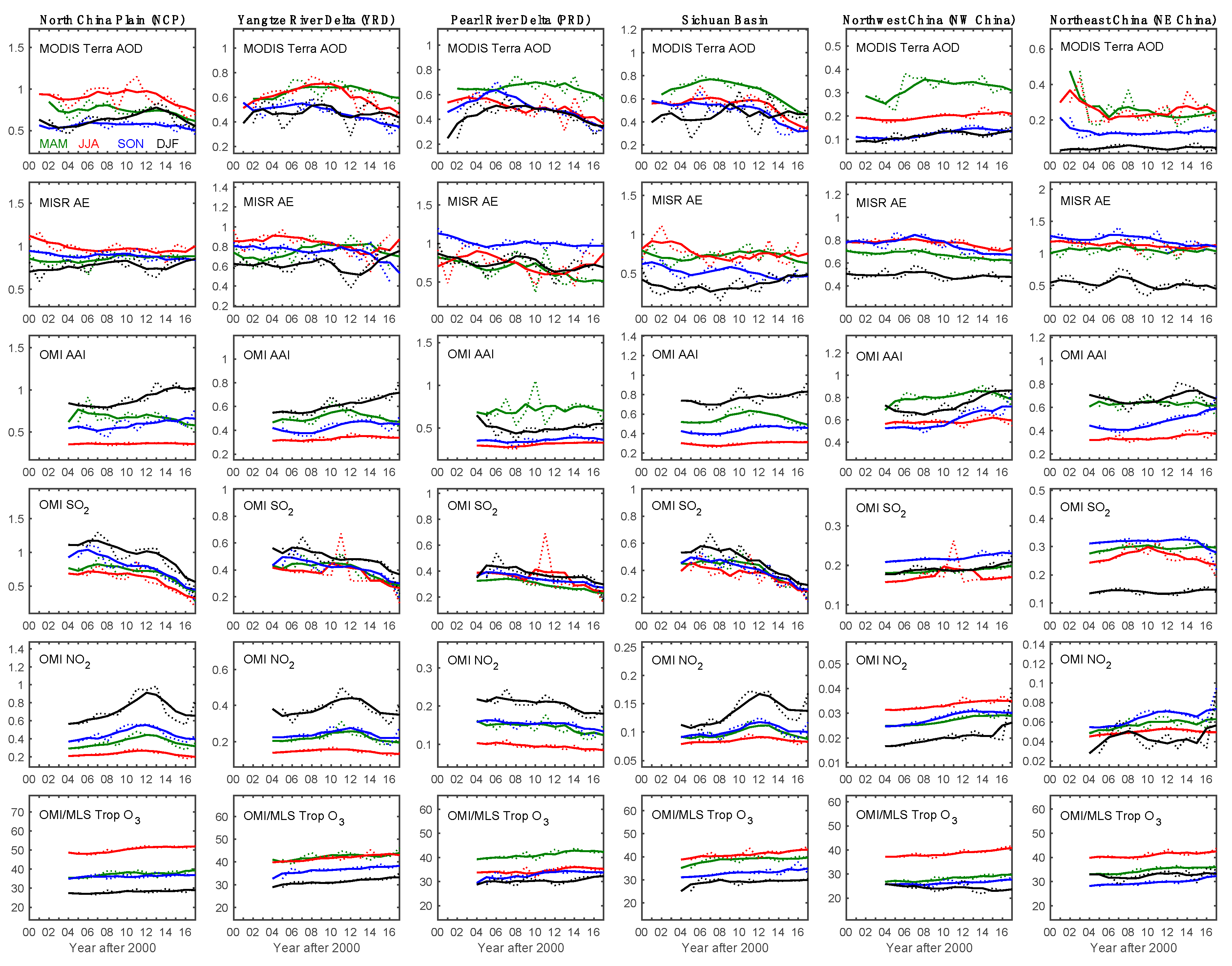
As aerosol properties and pollution composition have different seasonal variability over different regions, we also examined the seasonal changes in detail. Figure 18 shows the seasonal time series for the six variables over the six representative regions. Although a glance of Figure 16 mostly indicates consistency with annual trends, more careful examination shows considerable differences in the seasonal trends. The difference in AOD trends tends to be larger than trace gases, which is reasonable, since AOD involves the complicated mixing of different species. Over the NCP, the start of the AOD decrease for the winter season (DJF) clearly lags behind the other three seasons, and the variability of the AOD time series appears more consistent with that of NO2 than those of SO2 and AAI. This suggests that changes in nitrate aerosols are likely to be responsible for the winter AOD trends in this region. The increase of AAI might also contribute to the lagged decline of winter aerosol loading and the near flat aerosol trend in the fall (SON). For the YRD, the strongest decline in AOD as large as 0.3/decade occurred in the summer season (JJA) after 2008; spring and fall also showed a moderate decrease, whereas the winter AOD time series was generally flat. Although SO2 and NO2 reduction can lead to a significant decrease of sulfate and nitrate aerosols, respectively, the increase of absorbing aerosols in the winter and fall as reflected in the positive AAI trends may compensate for this decrease. For the PRD region, summer and fall AOD exhibited a consistent decline from 2000 to 2018, whereas winter and spring AOD first increased until ~2008 and then decreased. This difference might be related to meteorology and biomass burning aerosols transported from Southeast Asia [60,70]. The Sichuan Basin showed consistent AOD changes except for winter, when a flat AOD time series was observed. Unlike the other three seasons, the winter season suffered from an increase in both AAI and AE, which indicated that the AOD decrease caused by SO2 and NO2 reduction might have been compensated by an increase in fine mode absorbing aerosols, mostly black and organic carbon. NW China is primarily dominated by dust aerosols, and the AOD values were clearly much higher in the dust-peak season of spring. However, the AOD for the non-peak seasons (i.e., summer, autumn, and winter) all increased at ~0.03/decade while that for spring first increased rapidly at 0.1/decade until ~2008, but then slightly decreased by ~0.05 from 2008 to 2016. Meanwhile, the SO2 and NO2 concentrations also showed consistent increases, unlike East China. As discussed above, this might be related to the western development policy. An increase in anthropogenic aerosols should be responsible for the AOD increase during the non-peak seasons, whereas the dust change is most likely to be related to natural variability. The last region, NE China, is dominated by heavy industries and anthropogenic aerosols should be the major component. Unlike most East China regions, its AOD for all seasons except winter first showed clear decreases from 2000 to ~2006 by ~0.15, but remained flat afterward. Winter AOD showed weak and consistent upward trends (~0.04/decade). Additionally, unlike East China, no obvious reduction in SO2 and NO2 concentrations were found over this region, and NO2 even increased for the winter and fall. Pollution control here might not have been implemented as strictly as East China, which led to the insignificant or even positive AOD trends. Finally, it should be noted that the changes in the loading of aerosols and trace gases can be associated with changes in both emissions and meteorology. In the future, we plan to carry out a series of detailed studies involving both data analysis and model simulations to attribute the trends.
4. Discussions
Our study is not the first to report the pollution trends in China. Previous studies have also noticed similar trends or change in AOD [56,71] or trace gases [20,72]. However, these studies mostly used a single set of satellite data or/and focused on a particular region. Our study was the first to conduct a comprehensive spatial analysis of pollution changes in China using multiple satellite datasets. The consistency of different datasets not only increases the robustness of the results, but also provides valuable insights into the compositional changes. Compared to previous studies, our study offers a few new findings. (1) While previous studies have mostly focused on the most densely populated regions such as the NCP, YRD, and PRD, we showed that aerosol loading over NW and NE China has increased. This is most likely the result of increased dust, according to the positive AAI trends and negative AE trends. However, from the slight increase of SO2 and NO2, we can infer that sulfate and nitrate aerosols may also play a role. (2) Many studies revealed the recent pollution reduction in East China, but the shift from positive to negative trends was different for different regions and for different pollutants. In particular, the pollution decline for the YRD and PRD started in ~2008, whereas for the NCP and the Sichuan Basin, it started around ~2012. A further comparison with SO2 and NO2 trends indicates that the YRD and PRD trends were more consistent with the SO2 trends, while for the NCP and the Sichuan Basin, it was in phase with the NO2 trends. (3) Previous study (e.g., [66]) about tropospheric O3 trends have only used surface observations, therefore the analysis was focused on the east part because there were very few monitoring sites in West China. By using satellite data, we showed that there were also significant increases in tropospheric O3 for West China, even over the Tibetan Plateau. The trends also exhibited distinct seasonal features. These findings highlight the usefulness and importance of satellites in environmental monitoring and research.
The cause of the observed trends, nonetheless, still needs investigation. The decrease of SO2, NO2, and AOD is likely to be the result of a series of emission reduction strategies taken by China. However, meteorology may also play an important role [73], especially concerning natural sources. In the future, we will be further quantifying different effects using chemical transport models. We will also examine the interannual variability and regional differences of pollution changes in detail.
5. Conclusions
In this study, we analyzed trends of major pollutants in China including aerosols, SO2, NO2, and tropospheric ozone using multiple satellite retrieval datasets. The major conclusions include:
- (1)
- Total aerosol loading in China, especially in the eastern and southern parts, has exhibited a significant decrease of ~0.15–0.3/decade since 2008, after an almost decade-long increase.
- (2)
- This negative trend is accompanied by decreases of SO2 and NO2 during the same period, suggesting reductions in anthropogenic emissions.
- (3)
- NW and NE China, however, exhibit weak positive AOD trends at ~0.1/decade, together with significant positive AAI and negative AE trends. These combined indicate that dust aerosol loading has likely increased and caused a total AOD increase over these two regions.
- (4)
- Multiple regression of AOD against AAI, SO2, and NO2 show overall successful fitting and reasonable spatial distribution of the coefficients, further supporting the inferred compositional changes associated with the AOD trends.
- (5)
- Unlike aerosols, tropospheric ozone exhibits near uniform significant upward trends all over China, implying that ozone pollution control remains a challenging problem.
Funding
This study was funded by the National Key Research and Development Program of China, No. 2017YFC0212803 and by the National Natural Science Foundation of China (NSFC Nos. 41575018 and 41975023).
Acknowledgments
We thank the MODIS, MISR, OMI, and OMI/MLS teams and the PIs of Beijing and XiangHe AERONET sites for providing the data used in this study. The MODIS AOD data were downloaded from https://ladsweb.modaps.eosdis.nasa.gov/. The MISR AOD and AE data were downloaded from http://eosweb.larc.nasa.gov. OMI AAI, SO2, and NO2 products were obtained from https://disc.gsfc.nasa.gov/. The OMI/MLS tropospheric ozone data were downloaded from https://acd-ext.gsfc.nasa.gov/Data_services/cloud_slice/#nd. The AERONET data for Beijing and XiangHe were provided by the AERONET website at https://aeronet.gsfc.nasa.gov/.
Conflicts of Interest
The author declares no conflict of interests.
Abbreviations
| AAI | Absorbing Aerosol Index |
| AE | Angstrom Exponent |
| AERONET | Aerosol Robotic Network |
| AOD | aerosol optical depth |
| DJF | December, January, February |
| EOS | Earth Observing Systems |
| JJA | June, July, August |
| MAM | March, April, May |
| MISR | Multi-angle Imaging Spectroradiometer |
| MLS | Microwave Limb Sounder |
| MODIS | Moderate Resolution Imaging Spectroradiometer |
| NCP | North China Plain |
| NE China | Northeast China |
| NW China | Northwest China |
| OMI | Ozone Monitoring Instrument |
| PBLH | Planetary Boundary Layer Height |
| PRD | Pearl River Delta |
| SON | September, October, November |
| YRD | Yangtze River Delta |
References
- Kan, H.; Chen, R.; Tong, S. Ambient air pollution, climate change, and population health in China. Environ. Int. 2012, 42, 10–19. [Google Scholar] [CrossRef] [PubMed]
- Kasoar, M.; Voulgarakis, A.; Lamarque, J.-F.; Shindell, D.T.; Bellouin, N.; Collins, W.J.; Faluvegi, G.; Tsigaridis, K. Regional and global temperature response to anthropogenic SO2 emissions from China in three climate models. Atmos. Chem. Phys. 2016, 16, 9785–9804. [Google Scholar] [CrossRef] [Green Version]
- Zhang, H.; Zhang, B.; Bi, J. More efforts, more benefits: Air pollutant control of coal-fired power plants in China. Energy 2015, 80, 1–9. [Google Scholar] [CrossRef]
- Chan, C.K.; Yao, X. Air pollution in mega cities in China. Atmos. Environ. 2008, 42, 1–42. [Google Scholar] [CrossRef]
- Ma, Q.; Cai, S.; Wang, S.; Zhao, B.; Martin, R.V.; Brauer, M.; Cohen, A.; Jiang, J.; Zhou, W.; Hao, J.; et al. Impacts of coal burning on ambient PM2.5 pollution in China. Atmos. Chem. Phys. 2017, 17, 4477–4491. [Google Scholar] [CrossRef] [Green Version]
- Rohde, R.A.; Muller, R.A. Air Pollution in China: Mapping of Concentrations and Sources. PLoS ONE 2015, 10, e0135749. [Google Scholar] [CrossRef]
- Qin, Y.M.; Tan, H.B.; Li, Y.J.; Schurman, M.I.; Li, F.; Canonaco, F.; Prévôt, A.S.H.; Chan, C.K. Impacts of traffic emissions on atmospheric particulate nitrate and organics at a downwind site on the periphery of Guangzhou, China. Atmos. Chem. Phys. 2017, 17, 10245–10258. [Google Scholar] [CrossRef] [Green Version]
- Zhang, L.; Liu, L.; Zhao, Y.; Gong, S.; Zhang, X.; Henze, D.K.; Wang, Y. Source attribution of particulate matter pollution over North China with the adjoint method. Environ. Res. Lett. 2015, 10. [Google Scholar] [CrossRef]
- Zhang, X.; Rao, R.; Huang, Y.; Mao, M.; Berg, M.J.; Sun, W. Black carbon aerosols in urban central China. J. Quant. Spectrosc. Radiat. Transf. 2015, 150, 3–11. [Google Scholar] [CrossRef]
- Li, K.; Liao, H.; Mao, Y.; Ridley, D.A. Source sector and region contributions to concentration and direct radiative forcing of black carbon in China. Atmos. Environ. 2016, 124, 351–366. [Google Scholar] [CrossRef]
- Chen, J.; Li, C.; Ristovski, Z.; Milic, A.; Gu, Y.; Islam, M.S.; Guo, H. A review of biomass burning: Emissions and impacts on air quality, health and climate in China. Sci. Total Environ. 2017, 579, 1000–1034. [Google Scholar] [CrossRef] [Green Version]
- Wang, X.; Dong, Z.; Zhang, J.; Liu, L. Modern dust storms in China: An overview. J. Arid Environ. 2004, 58, 559–574. [Google Scholar] [CrossRef]
- Li, X.; Liu, J.; Mauzerall, D.L.; Emmons, L.K.; Walters, S.; Horowitz, L.W.; Tao, S. Effects of trans-Eurasian transport of air pollutants on surface ozone concentrations over Western China. J. Geophys. Res. Atmos. 2014, 119, 12–338. [Google Scholar] [CrossRef]
- Zhao, Z.; Cao, J.; Shen, Z.; Xu, B.; Zhu, C.; Chen, L.W.A.; Su, X.; Liu, S.; Han, Y.; Wang, G.; et al. Aerosol particles at a high-altitude site on the Southeast Tibetan Plateau, China: Implications for pollution transport from South Asia. J. Geophys. Res. Atmos. 2013, 118, 11360–11375. [Google Scholar] [CrossRef]
- Chan, C.Y.; Chan, L.Y.; Harris, J.M.; Oltmans, S.J.; Blake, D.R.; Qin, Y.; Zheng, Y.G.; Zheng, X.D. Characteristics of biomass burning emission sources, transport, and chemical speciation in enhanced springtime tropospheric ozone profile over Hong Kong. J. Geophys. Res. 2003, 108, 4015. [Google Scholar] [CrossRef] [Green Version]
- Chan, C.Y.; Wong, K.H.; Li, Y.S.; Chan, L.Y.; Zheng, X.D. The effects of Southeast Asia fire activities on tropospheric ozone, trace gases and aerosols at a remote site over the Tibetan Plateau of Southwest China. Tellus B Chem. Phys. Meteorol. 2006, 58, 310–318. [Google Scholar] [CrossRef] [Green Version]
- De Foy, B.; Lu, Z.; Streets, D.G. Satellite NO2 retrievals suggest China has exceeded its NOx reduction goals from the twelfth Five-Year Plan. Sci. Rep. 2016, 6, 35912. [Google Scholar] [CrossRef] [PubMed] [Green Version]
- Georgoulias, A.K.; Stammes, P.; Boersma, K.F.; Eskes, H.J. Trends and trend reversal detection in 2 decades of tropospheric NO2 satellite observations. Atmos. Chem. Phys. 2019, 19, 6269–6294. [Google Scholar] [CrossRef] [Green Version]
- Liu, F.; Zhang, Q.; Zheng, B.; Tong, D.; Yan, L.; Zheng, Y.; He, K. Recent reduction in NOx emissions over China: Synthesis of satellite observations and emission inventories. Environ. Res. Lett. 2016, 11, 114002. [Google Scholar] [CrossRef] [Green Version]
- Mijling, B.; Ding, J.; Koukouli, M.E.; Liu, F.; Li, Q.; Mao, H.; Theys, N. Cleaning up the air: Effectiveness of air quality policy for SO2 and NOx emissions in China. Atmos. Chem. Phys. 2017, 17, 1775–1789. [Google Scholar] [CrossRef] [Green Version]
- Wang, S.; Zhang, Q.; Martin, R.V.; Philip, S.; Liu, F.; Li, M.; Jiang, X.; He, K. Satellite measurements oversee China’s sulfur dioxide emission reductions from coal-fired power plants. Environ. Res. Lett. 2015, 10, 114015. [Google Scholar] [CrossRef] [Green Version]
- Ma, Z.; Liu, R.; Liu, Y.; Bi, J. Effects of air pollution control policies on PM2.5 pollution improvement in China from 2005 to 2017: A satellite-based perspective. Atmos. Chem. Phys. 2019, 19, 6861–6877. [Google Scholar] [CrossRef] [Green Version]
- Torres, O.; Bhartia, P.K.; Herman, J.R.; Ahmad, Z.; Gleason, J. Derivation of aerosol properties from satellite measurements of backscattered ultraviolet radiation: Theoretical basis. J. Geophys. Res. Atmos. 1998, 103, 17099–17110. [Google Scholar] [CrossRef]
- Wang, T.; Xue, L.; Brimblecombe, P.; Lam, Y.F.; Li, L.; Zhang, L. Ozone pollution in China: A review of concentrations, meteorological influences, chemical precursors, and effects. Sci. Total Environ. 2017, 575, 1582–1596. [Google Scholar] [CrossRef] [PubMed]
- Ma, Z.; Xu, J.; Quan, W.; Zhang, Z.; Lin, W.; Xu, X. Significant increase of surface ozone at a rural site, north of eastern China. Atmos. Chem. Phys. 2016, 16, 3969–3977. [Google Scholar] [CrossRef] [Green Version]
- Levy, R.C.; Mattoo, S.; Munchak, L.A.; Remer, L.A.; Sayer, A.M.; Patadia, F.; Hsu, N.C. The Collection 6 MODIS aerosol products over land and ocean. Atmos. Meas. Tech. 2013, 6, 2989–3034. [Google Scholar] [CrossRef] [Green Version]
- Available online: https://ladsweb.modaps.eosdis.nasa.gov/ (accessed on 15 October 2019).
- Levy, R.C.; Leptoukh, G.G.; Kahn, R.; Zubko, V.; Gopalan, A.; Remer, L.A. A Critical Look at Deriving Monthly Aerosol Optical Depth from Satellite Data. IEEE Trans. Geosci. Remote Sens. 2009, 47, 2942–2956. [Google Scholar] [CrossRef]
- Diner, D.J.; Beckert, J.C.; Reilly, T.H.; Bruegge, C.J.; Conel, J.E.; Kahn, R.A.; Martonchik, J.V.; Ackerman, T.P.; Davies, R.; Gerstl, S.A.; et al. Multi-angle Imaging SpectroRadiometer (MISR) instrument description and experiment overview. IEEE Trans. Geosci. Remote Sens. 1998, 36, 1072–1087. [Google Scholar] [CrossRef]
- Martonchik, J.V.; Kahn, R.A.; Diner, D.J. Retrieval of aerosol properties over land using MISR observations. In Satellite Aerosol Remote Sensing Over Land; Springer: Berlin/Heidelberg, Germany, 2009; pp. 267–293. [Google Scholar]
- Kahn, R.A.; Nelson, D.L.; Garay, M.J.; Levy, R.C.; Bull, M.A.; Diner, D.J.; Martonchik, J.V.; Paradise, S.R.; Hansen, E.G.; Remer, L.A. MISR aerosol product attributes and statistical comparisons with MODIS. IEEE Trans. Geosci. Remote Sens. 2009, 47, 4095–4114. [Google Scholar] [CrossRef]
- Available online: http://eosweb.larc.nasa.gov (accessed on 15 October 2019).
- Kahn, R.A.; Gaitley, B.J.; Martonchik, J.V.; Diner, D.J.; Crean, K.A.; Holben, B. Multiangle Imaging Spectroradiometer (MISR) global aerosol optical depth validation based on 2 years of coincident Aerosol Robotic Network (AERONET) observations. J. Geophys. Res. Atmos. 2005, 110. [Google Scholar] [CrossRef] [Green Version]
- Kahn, R.A.; Gaitley, B.J.; Garay, M.J.; Diner, D.J.; Eck, T.F.; Smirnov, A.; Holben, B.N. Multiangle Imaging SpectroRadiometer global aerosol product assessment by comparison with the Aerosol Robotic Network. J. Geophys. Res. Atmos. 2010, 115. [Google Scholar] [CrossRef]
- Levelt, P.F.; van den Oord, G.H.; Dobber, M.R.; Malkki, A.; Visser, H.; de Vries, J.; Stammes, P.; Lundell, J.O.; Saari, H. The ozone monitoring instrument. IEEE Trans. Geosci. Remote Sens. 2006, 44, 1093–1101. [Google Scholar] [CrossRef]
- Torres, O.; Tanskanen, A.; Veihelmann, B.; Ahn, C.; Braak, R.; Bhartia, P.K.; Veefkind, P.; Levelt, P. Aerosols and surface UV products from Ozone Monitoring Instrument observations: An overview. J. Geophys. Res. Atmos. 2007, 112. [Google Scholar] [CrossRef] [Green Version]
- Torres, O.; Ahn, C.; Chen, Z. Improvements to the OMI near-UV aerosol algorithm using A-train CALIOP and AIRS observations. Atmos. Meas. Tech. 2013, 6, 3257–3270. [Google Scholar] [CrossRef] [Green Version]
- Available online: https://disc.gsfc.nasa.gov/ (accessed on 15 October 2019).
- Prospero, J.M.; Ginoux, P.; Torres, O.; Nicholson, S.E.; Gill, T.E. Environmental characterization of global sources of atmospheric soil dust derived from the NIMBUS-7 TOMS absorbing aerosol product. Rev. Geophys. 2002, 40, 1002. [Google Scholar] [CrossRef]
- Krotkov, N.A.; Carn, S.A.; Krueger, A.J.; Bhartia, P.K.; Yang, K. Band residual difference algorithm for retrieval of SO2 from the aura ozone monitoring instrument (OMI). IEEE Trans. Geosci. Remote Sens. 2006, 44, 1259–1266. [Google Scholar] [CrossRef]
- Krotkov, N.A.; Lamsal, L.N.; Celarier, E.A.; Swartz, W.H.; Marchenko, S.V.; Bucsela, E.J.; Chan, K.L.; Wenig, M.; Zara, M. The version 3 OMI NO2 standard product. Atmos. Meas. Tech. 2017, 10, 3133–3149. [Google Scholar] [CrossRef] [Green Version]
- Li, C.; Joiner, J.; Krotkov, N.A.; Bhartia, P.K. A fast and sensitive new satellite SO2 retrieval algorithm based on principal component analysis: Application to the ozone monitoring instrument. Geophys. Res. Lett. 2013, 40, 6314–6318. [Google Scholar] [CrossRef] [Green Version]
- Krotkov, N.A.; McClure, B.; Dickerson, R.R.; Carn, S.A.; Li, C.; Bhartia, P.K.; Yang, K.; Krueger, A.J.; Li, Z.; Levelt, P.F.; et al. Validation of SO2 retrievals from the Ozone Monitoring Instrument over NE China. J. Geophys. Res. 2008, 113. [Google Scholar] [CrossRef]
- Marchenko, S.; Krotkov, N.A.; Lamsal, L.N.; Celarier, E.A.; Swartz, W.H.; Bucsela, E.J. Revising the slant column density retrieval of nitrogen dioxide observed by the Ozone Monitoring Instrument. J. Geophys. Res. Atmos. 2015, 120, 5670–5692. [Google Scholar] [CrossRef] [Green Version]
- Available online: https://acd-ext.gsfc.nasa.gov/Data_services/cloud_slice/#nd (accessed on 15 October 2019).
- Ziemke, J.R.; Chandra, S.; Duncan, B.N.; Froidevaux, L.; Bhartia, P.K.; Levelt, P.F.; Waters, J.W. Tropospheric ozone determined from Aura OMI and MLS: Evaluation of measurements and comparison with the Global Modeling Initiative’s Chemical Transport Model. J. Geophys. Res. Atmos. 2006, 111. [Google Scholar] [CrossRef]
- Ziemke, J.R.; Chandra, S.; Labow, G.J.; Bhartia, P.K.; Froidevaux, L.; Witte, J.C. A global climatology of tropospheric and stratospheric ozone derived from Aura OMI and MLS measurements. Atmos. Chem. Phys. 2011, 11, 9237–9251. [Google Scholar] [CrossRef] [Green Version]
- Sen, P.K. Estimates of the regression coefficient based on Kendall’s tau. J. Am. Stat. Assoc. 1968, 63, 1379–1389. [Google Scholar] [CrossRef]
- Mann, H.B. Nonparametric tests against trend. Econometrica 1945, 13, 245–259. [Google Scholar] [CrossRef]
- Kendall, M.G. Rank Correlation Methods; Griffin: London, UK, 1975. [Google Scholar]
- von Storch, V.H. Misuses of statistical analysis in climate research. In Analysis of Climate Variability: Applications of Statistical Techniques; Von Storch, H., Navarra, A., Eds.; Springer: Berlin, Germany, 1995; pp. 11–26. [Google Scholar]
- Yue, S.; Pilon, P.; Phinney, B.; Cavadias, G. The influence of autocorrelation on the ability to detect trend in hydrological series. Hydrol. Process. 2002, 16, 1807–1829. [Google Scholar] [CrossRef]
- Zhang, X.; Zwiers, F.W. Comment on “Applicability of prewhitening to eliminate the influence of serial correlation on the Mann-Kendall test” by Sheng Yue and Chun Yuan Wang. Water Resour. Res. 2004, 40. [Google Scholar] [CrossRef] [Green Version]
- Belsley, D. Conditioning Diagnostics: Collinearity and Weak Data in Regression; Wiley: New York, NY, USA, 1991; ISBN 978-0-471-52889-0. [Google Scholar]
- Chatterjee, S.; Hadi, A.S.; Price, B. Regression Analysis by Example, 3rd ed.; John Wiley and Sons: New York, NY, USA, 2000; ISBN 978-0-471-31946-7. [Google Scholar]
- Zhang, J.; Reid, J.S.; Alfaro-Contreras, R.; Xian, P. Has China been exporting less particulate air pollution over the past decade. Geophys. Res. Lett. 2017, 44, 2941–2948. [Google Scholar] [CrossRef]
- Holben, B.N.; Tanre, D.; Smirnov, A.; Eck, T.F.; Slutsker, I.; Abuhassan, N.; Newcomb, W.W.; Schafer, J.S.; Chatenet, B.; Lavenu, F.; et al. An emerging ground-based aerosol climatology: Aerosol optical depth from AERONET. J. Geophys. Res. Atmos. 2001, 106, 12067–12097. [Google Scholar] [CrossRef]
- Guo, J.P.; Zhang, X.Y.; Wu, Y.R.; Zhaxi, Y.; Che, H.Z.; La, B.; Li, X.W. Spatio-temporal variation trends of satellite-based aerosol optical depth in China during 1980–2008. Atmos. Environ. 2011, 45, 6802–6811. [Google Scholar] [CrossRef]
- Mukai, M.; Nakajima, T.; Takemura, T. A study of long-term trends in mineral dust aerosol distributions in Asia using a general circulation model. J. Geophys. Res. 2004, 109, D19204. [Google Scholar] [CrossRef]
- De Graaf, M.; Stammes, P.; Torres, O.; Koelemeijer, R.B.A. Absorbing Aerosol Index: Sensitivity analysis, application to GOME and comparison with TOMS. J. Geophys. Res. 2005, 110, D01201. [Google Scholar] [CrossRef] [Green Version]
- Mahowald, N.M.; Dufresne, J.-L. Sensitivity of TOMS aerosol index to boundary layer height: Implications for detection of mineral aerosol sources. Geophys. Res. Lett. 2004, 31. [Google Scholar] [CrossRef] [Green Version]
- Guo, J.; Li, Y.; Cohen, J.B.; Li, J.; Chen, D.; Xu, H.; Liu, L.; Yin, J.; Hu, K.; Zhai, P. Shift in the temporal trend of boundary layer height in China using long-term (1979–2016) radiosonde data. Geophys. Res. Lett. 2019, 46, 6080–6089. [Google Scholar] [CrossRef] [Green Version]
- Chen, C.; Park, T.; Wang, X.; Piao, S.; Xu, B.; Chaturvedi, R.K.; Fuchs, R.; Brovkin, V.; Ciais, P.; Fensholt, R.; et al. China and India lead in greening of the world through land-use management. Nat. Sustain. 2019, 2, 122. [Google Scholar] [CrossRef] [PubMed]
- Li, J.; Jiang, Y.; Xia, X.; Hu, Y. Increase of surface solar irradiance across East China related to changes in aerosol properties during the past decade. Environ. Res. Lett. 2018, 13. [Google Scholar] [CrossRef]
- Krotkov, N.A.; McLinden, C.A.; Li, C.; Lamsal, L.N.; Celarier, E.A.; Marchenko, S.V.; Swartz, W.H.; Bucsela, E.J.; Joiner, J.; Duncan, B.N.; et al. Aura OMI observations of regional SO2 and NO2 pollution changes from 2005 to 2015. Atmos. Chem. Phys. 2016, 16, 4605–4629. [Google Scholar] [CrossRef] [Green Version]
- Wang, Y.; Zhang, Y.; Hao, J.; Luo, M. Seasonal and spatial variability of surface ozone over China: Contributions from background and domestic pollution. Atmos. Chem. Phys. 2011, 11, 3511–3525. [Google Scholar] [CrossRef] [Green Version]
- Verstraeten, W.W.; Neu, J.L.; Williams, J.E.; Bowman, K.W.; Worden, J.R.; Boersma, K.F. Rapid increases in tropospheric ozone production and export from China. Nat. Geosci. 2015, 8, 690. [Google Scholar] [CrossRef]
- Sun, L.; Xue, L.; Wang, T.; Gao, J.; Ding, A.; Cooper, O.R.; Lin, M.; Xu, P.; Wang, Z.; Wang, X.; et al. Significant increase of summertime ozone at Mount Tai in Central Eastern China. Atmos. Chem. Phys. 2016, 16, 10637–10650. [Google Scholar] [CrossRef] [Green Version]
- Li, K.; Jacob, D.J.; Liao, H.; Shen, L.; Zhang, Q.; Bates, K.H. Anthropogenic drivers of 2013–2017 trends in summer surface ozone in China. Proc. Natl. Acad. Sci. USA 2019, 116, 422–427. [Google Scholar] [CrossRef] [Green Version]
- Fu, J.S.; Hsu, N.C.; Gao, Y.; Huang, K.; Li, C.; Lin, N.-H.; Tsay, S.-C. Evaluating the influences of biomass burning during 2006 BASE-ASIA: A regional chemical transport modeling. Atmos. Chem. Phys. 2012, 12, 3837–3855. [Google Scholar] [CrossRef] [Green Version]
- Liu, X.; Chen, Q.; Che, H.; Zhang, R.; Gui, K.; Zhang, H.; Zhao, T. Spatial distribution and temporal variation of aerosol optical depth in the Sichuan basin, China, the recent ten years. Atmos. Environ. 2016, 147, 434–445. [Google Scholar] [CrossRef]
- Zhang, L.; Lee, C.S.; Zhang, R.; Chen, L. Spatial and temporal evaluation of long term trend (2005–2014) of OMI retrieved NO2 and SO2 concentrations in Henan Province, China. Atmos. Environ. 2017, 154, 151–166. [Google Scholar] [CrossRef]
- Wang, H.-J.; Chen, H.-P. Understanding the recent trend of haze pollution in eastern China: Roles of climate change. Atmos. Chem. Phys. 2016, 16, 4205–4211. [Google Scholar] [CrossRef] [Green Version]
Figure 1.
Spatial distribution of annual mean MODIS Terra AOD (a), MISR AE (b), OMI AAI (c), OMI SO2 (d) and NO2 (e), and OMI/MLS tropospheric O3 (f). The black boxes in panel (a) indicate the representative regions defined for regional analysis, namely NCP, NE China, NW China, YRD, PRD, and the Sichuan Basin.

Figure 2.
MODIS Terra (a–c), MODIS Aqua (d–f) and MISR (g–i) AOD trends over China for the 2000–2017 (a,d,g, 2002–2017 for MODIS Aqua), 2000–2007 (b,e,h, 2002–2017 for MODIS Aqua) and 2008–2017 (c,f,i) periods. The trends were calculated as the Sen’s slope and tested using the Mann–Kendall test. Trends with significance level >95% are marked with black dots. A clear transition from negative to positive trends was observed since 2008. The locations of Beijing and XiangHe AERONET sites are marked on panel (a).

Figure 3.
AERONET AOD time series and linear trends for Beijing and XiangHe. The dashed lines indicate linear trends fitted for the 2000–2007 and 2008–2017 periods using the Sen’s slope method. All trends were significant at 95% according to the Mann–Kendall test.
Figure 3.
AERONET AOD time series and linear trends for Beijing and XiangHe. The dashed lines indicate linear trends fitted for the 2000–2007 and 2008–2017 periods using the Sen’s slope method. All trends were significant at 95% according to the Mann–Kendall test.

Figure 4.
MODIS Terra AOD trends calculated during the 2000–2007 period for the four seasons: Spring—March, April, May (MAM); Summer—June, July, August (JJA); Fall—September, October, November (SON); Winter—December, January, February (DJF). The trends were calculated as the Sen’s slope and tested using the Mann–Kendall test. Trends with significance level >95% are marked with black dots.

Figure 5.
The same as Figure 4, but calculated during the 2008–2017 period.
Figure 5.
The same as Figure 4, but calculated during the 2008–2017 period.

Figure 6.
OMI AAI (a) and MISR AE (b) trends calculated for the 2005–2017 period. The trends were calculated as the Sen’s slope and tested using the Mann–Kendall test. Trends with significance level > 95% are marked with black dots.
Figure 6.
OMI AAI (a) and MISR AE (b) trends calculated for the 2005–2017 period. The trends were calculated as the Sen’s slope and tested using the Mann–Kendall test. Trends with significance level > 95% are marked with black dots.

Figure 7.
Seasonal OMI AAI trend for 2005–2017.

Figure 8.
OMI SO2 (a) and OMI NO2 (b) trends over China for the 2005–2017 period. The trends were calculated as the Sen’s slope and tested using the Mann–Kendall test. Trends with a significance level > 95% are marked with black dots.
Figure 8.
OMI SO2 (a) and OMI NO2 (b) trends over China for the 2005–2017 period. The trends were calculated as the Sen’s slope and tested using the Mann–Kendall test. Trends with a significance level > 95% are marked with black dots.

Figure 9.
Seasonal OMI SO2 trends for 2005–2017.

Figure 10.
Seasonal OMI NO2 trends for 2005–2017.

Figure 11.
Variance of AOD explained by the multiple regression model against AAI, SO2, and NO2. The significance of the regression was tested using the F test and places passing the 95% significance level are marked by black dots.
Figure 11.
Variance of AOD explained by the multiple regression model against AAI, SO2, and NO2. The significance of the regression was tested using the F test and places passing the 95% significance level are marked by black dots.

Figure 12.
Regression coefficients for AAI (a), SO2 (b), and NO2 (c) for the multiple regression model. Each individual coefficient was tested using the F test and places passing the 95% significance level are marked by black dots.
Figure 12.
Regression coefficients for AAI (a), SO2 (b), and NO2 (c) for the multiple regression model. Each individual coefficient was tested using the F test and places passing the 95% significance level are marked by black dots.

Figure 13.
Variance explained by the seasonal regression model.

Figure 14.
Distribution of the regression coefficients for AAI, SO2, and NO2 from the seasonal model.
Figure 14.
Distribution of the regression coefficients for AAI, SO2, and NO2 from the seasonal model.

Figure 15.
OMI/MLS tropospheric ozone trends over China for the 2005–2017 period. The trends were calculated as the Sen’s slope and tested using the Mann–Kendall test. Trends with a significance level > 95% are marked with black dots.
Figure 15.
OMI/MLS tropospheric ozone trends over China for the 2005–2017 period. The trends were calculated as the Sen’s slope and tested using the Mann–Kendall test. Trends with a significance level > 95% are marked with black dots.

Figure 16.
Seasonal OMI/MLS tropospheric ozone trends. The trends were calculated as the Sen’s slope and tested using the Mann–Kendall test. Trends with a significance level > 95% are marked with black dots.
Figure 16.
Seasonal OMI/MLS tropospheric ozone trends. The trends were calculated as the Sen’s slope and tested using the Mann–Kendall test. Trends with a significance level > 95% are marked with black dots.

Figure 17.
Regional mean time series for all variables averaged over the six representative regions marked on Figure 1a. The thin gray lines are the original annual mean time series and the thick black lines are four year moving average smoothed time series. The relative changes for different periods are marked on each panel, with positive changes indicated in red and negative in blue.

Figure 18.
Similar to Figure 15, but showing the seasonal time series. The dotted lines represent annual time series and the solid lines show the four year running means.
Figure 18.
Similar to Figure 15, but showing the seasonal time series. The dotted lines represent annual time series and the solid lines show the four year running means.

© 2020 by the author. Licensee MDPI, Basel, Switzerland. This article is an open access article distributed under the terms and conditions of the Creative Commons Attribution (CC BY) license (http://creativecommons.org/licenses/by/4.0/).
Share and Cite
MDPI and ACS Style
Li, J. Pollution Trends in China from 2000 to 2017: A Multi-Sensor View from Space. Remote Sens. 2020, 12, 208. https://0-doi-org.brum.beds.ac.uk/10.3390/rs12020208
AMA Style
Li J. Pollution Trends in China from 2000 to 2017: A Multi-Sensor View from Space. Remote Sensing. 2020; 12(2):208. https://0-doi-org.brum.beds.ac.uk/10.3390/rs12020208
Chicago/Turabian StyleLi, Jing. 2020. "Pollution Trends in China from 2000 to 2017: A Multi-Sensor View from Space" Remote Sensing 12, no. 2: 208. https://0-doi-org.brum.beds.ac.uk/10.3390/rs12020208
Note that from the first issue of 2016, this journal uses article numbers instead of page numbers. See further details here.