Grouping-Based Time-Series Model for Monitoring of Fall Peak Coloration Dates Using Satellite Remote Sensing Data


1
State Key Laboratory of Information Engineering in Surveying, Mapping and Remote Sensing, Wuhan University, Wuhan 430079, China
2
School of Remote Sensing and Information Engineering, Wuhan University, Wuhan 430079, China
*
Author to whom correspondence should be addressed.
Remote Sens. 2020, 12(2), 274; https://0-doi-org.brum.beds.ac.uk/10.3390/rs12020274
Submission received: 18 December 2019
/
Revised: 7 January 2020
/
Accepted: 12 January 2020
/
Published: 14 January 2020
(This article belongs to the Special Issue Monitoring of Forest Ecological Environment Based on Remote Sensing Technology)
Abstract
:Accurate monitoring of plant phenology is vital to effective understanding and prediction of the response of vegetation ecosystems to climate change. Satellite remote sensing is extensively employed to monitor vegetation phenology. However, fall phenology, such as peak foliage coloration, is less well understood compared with spring phenological events, and is mainly determined using the vegetation index (VI) time-series. Each VI only emphasizes a single vegetation property. Thus, selecting suitable VIs and taking advantage of multiple spectral signatures to detect phenological events is challenging. In this study, a novel grouping-based time-series approach for satellite remote sensing was proposed, and a wide range of spectral wavelengths was considered to monitor the complex fall foliage coloration process with simultaneous changes in multiple vegetation properties. The spatial and temporal scale effects of satellite data were reduced to form a reliable remote sensing time-series, which was then divided into groups, namely pre-transition, transition and post-transition groups, to represent vegetation dynamics. The transition period of leaf coloration was correspondingly determined to divisions with the smallest intra-group and largest inter-group distances. Preliminary results using a time-series of Moderate Resolution Imaging Spectroradiometer (MODIS) data from 2002 to 2013 at the Harvard Forest (spatial scale: ~3500 m; temporal scale: ~8 days) demonstrated that the method can accurately determine the coloration period (correlation coefficient: 0.88; mean absolute difference: 3.38 days), and that the peak coloration periods displayed a shifting trend to earlier dates. The grouping-based approach shows considerable potential in phenological monitoring using satellite time-series.
1. Introduction
Vegetation phenological events, which play a crucial role in determining spatial and temporal patterns of net primary production, are highly sensitive to climate change [1]. The seasonal and long-time-scale dynamics in vegetation foliage parameterizes models used to understand the dynamic processes of earth ecosystems [2] and reflect the interactions between the terrestrial biosphere and the climate system [3]. Although a large number of growing season phenological events have been extensively explored [4], fall phenology remains poorly understood [5]; such knowledge is important to gain insights into the climate system and ecosystem management, because it can help in choosing suitable species to be planted according to the climate conditions [6]. Peak foliage coloration, which is one of the fall phenological events, is sensitive to environmental conditions, such as temperatures, water, and protein [7]. Therefore, accurate monitoring of peak foliage coloration is important to understand the underlying mechanisms and establish explicit phenological models with regard to climate change phenomena.
Satellite remote sensing provides unprecedented opportunities to monitor vegetation dynamics, including peak foliage coloration at large scales, because of the various spatial and temporal coverages of satellite observations [8]. Over the past decade, various methods based on satellite remote sensing data have been widely used to monitor vegetation phenology [9]. Satellite time-series of vegetation indices (VIs), such as the normalized difference vegetation index (NDVI), leaf area index (LAI), and enhanced vegetation index (EVI), which provide indicators of vegetation phenological stages, are widely used to identify phenological dates [10,11]. Moderate-resolution sensors, such as the Moderate Resolution Imaging Spectroradiometer (MODIS), the Medium Resolution Imaging Spectrometer (MERIS), the Advanced Very High-Resolution Radiometer (AVHRR), and the Visible Infrared Imager Radiometer Suite (VIIRS), allow calculation of near-daily frequency VIs to monitoring regional to global vegetation phenology [9].
The VI time-series is used to estimate phenological events using various approaches, including autoregressive moving average methods [12], the change rate of curvature methods [11], wavelet and Fourier transform methods [10], and threshold-based methods [13]. However, the various approaches result in dramatically different identified phenological transition dates, which may eventually lead to conflicting conclusions in the analysis of interactions between vegetation and climate change [14]. The different VIs emphasize varied vegetation properties and are sensitive to the soil, vegetation, and atmospheric conditions, making it challenging to select the appropriate VI to estimate phenological transition dates [15]. Leaf phenological processes can be better characterized by satellite remote sensing using multiple spectral wavelengths [16]. Tracking the change in multiple spectral signatures by combining different vegetation properties may outperform the tracking of a single VI time-series trajectory and can accurately estimate the transition dates of complex leaf coloration [16].
To better monitor the complex foliage coloration processes, Diao [16] developed a pheno-network model to detect peak coloration transition dates using collections of spectral signatures. In this model, MODIS time-series data were presented as nodes and edges to construct the network graph, and peak coloration dates were determined by the network metrics. However, the network-based model was complex and involved selections of a threshold, which is crucial to the network construction, indicating that the model performance is sensitive to the threshold selection. In addition, phenological models should be validated against field measurements. The scale effects (spatial and temporal scales) should be addressed to match the remote sensing images and field measurements [17] because in-situ observations are typically conducted locally [18,19] and many broad-leaf and deciduous forest species differ spatially inside small forest stands [7]. Generally, the mean values at the center of an empirical spatial or temporal window are used to match the in-situ measurements and avoid irregular satellite data.
To avoid threshold selection and take advantage of multiple spectral signatures, we proposed an innovative grouping-based method for peak foliage coloration estimations using MODIS data and field measurements from 2002 to 2013 at Harvard Forest. We considered the fall foliage transition dates as variables and divided the time-series data into three groups according to the assumed transition dates, namely pre-transition, transition, and post-transition groups. The most appropriate transition dates correspond to the minimum intra-group and largest inter-group distances. To reduce the scale effects, the optimal spatial and temporal scales for processing satellite data were determined based on semi-variance function [20]. The grouping-based approach with scale effects considered here may provide a new perspective in monitoring the foliage transition dates for fall peak coloration. Thus, the performance of the grouping-based model was also evaluated in this study.
2. Data and Methods
2.1. Data Sources and Preprocessing
Abundant field measurements of fall foliage peak coloration at Harvard Forest (42.54° N, 72.18° W, central Massachusetts, approximately 1500 m × 1500 m) are freely available. The region is located in the northeastern United States. Deciduous plants have been phenologically monitored in this region since 1991 at a frequency of 3–7 days (http://harvardforest.fas.harvard.edu/data-archives). The percentage of leaf coloration and percentage of leaf fall for each individual tree are observed during the field campaigns.
The MODIS data were used to estimate the peak coloration dates at Harvard Forest because MODIS provides an excellent opportunity to study regional-to-global scale land surface phenology with a high frequency [21]. The 2002–2013 MODIS data at Harvard Forest were downloaded from the Land Processes Distributed Active Archive Center (LP DAAC, https://lpdaac.usgs.gov/), including the Nadir Bidirectional reflectance distribution function (BRDF) Adjusted Reflectance data (NBAR, version 6), the MODIS BRDF/Albedo Quality data (BAQ, version 6), the MODIS Land Surface Temperature data (LST, version 6), and the MODIS Land Cover Type data (LCT, version 5.1). The role of each MODIS dataset in this study is summarized in Table 1.
The mean values of the species-based field observations were used to match the satellite images. To represent the continuous phenological stage, the field measurements were linearly interpolated for the missing dates. The mean peak coloration period at Harvard Forest based on the field measurements was obtained from Diao [16]. The seven spectral bands (from visible to shortwave infrared) of the NBAR time-series data were used as the main data source to determine the fall peak coloration transition dates. The BAQ data, LST data (resampled to 500 m using nearest-neighbor interpolation), and LCT data were used to eliminate the invalid pixels such as pixels covered by snow or clouds. The mean peak coloration periods at Harvard Forest obtained from field measurements were compared with the results estimated using satellite remote sensing to evaluate the performance of our proposed method. More details regarding the preprocessing of the field measurements and MODIS data can be found in Diao [16]. The preprocessing steps of MODIS data are summarized in Figure 1.
2.2. Determination of Optimal Spatial and Temporal Scales
A spatial window is required to match the MODIS data and field measurements and avoid spatial uncertainty [18]. To reduce the influence of irregular points in a time-series, a temporal window is needed [16]. The scale choice of remote sensing data is one of the fundamental factors that should be considered to provide the most suitable level of information for remote sensing applications [19]. The optimal sampling scale is highly related to the spatial and temporal characteristics of ground targets. Low or high scales will lead to insufficient information or information redundancy, which will influence the analysis and interpretations of satellite remote sensing [8,18].
The most commonly used methods to determine the optimal sampling scale are based on geostatistical methods [22]. Semi-variance is one of the comprehensive indicators to describe dependence and heterogeneity quantitatively and determine an optimal sampling scale which is defined as [20]:
where is the scale for isotropic variation; is the nugget; is the sill; and is the range, which represents the variation scale of geographical elements. Geographic variables with a scale larger than will no longer correlate, and can be regarded as the optimal scale. After the empirical semi-variance is calculated from satellite images, the can then be fitted, and is further determined. The semi-variance function was used to determine the optimal spatial and temporal scales for satellite images in this study.
To determine the spatial scale at Harvard Forest, the high-resolution atmospherically corrected surface reflectance data from Landsat-7/Enhanced Thematic Mapper Plus (ETM+, 30 m) of 2002–2013 were used which can efficiently represent the surface conditions and were obtained through the Google Earth Engine [23] with co-referencing or spatial accuracy tests performed. The high-frequency (daily) MODIS NBAR data with the influence of atmospheric interference and noise reduction were used to calculate the optimal temporal scale at Harvard Forest. The optimal spatial scale was firstly determined, and the NBAR data were then processed according to the optimal spatial scale to obtain the optimal temporal scale (see Figure 1). Specifically, the mean value within the optimal spatial scale was used to represent the value of the central pixel value.
2.3. Grouping-Based Time-Series Model
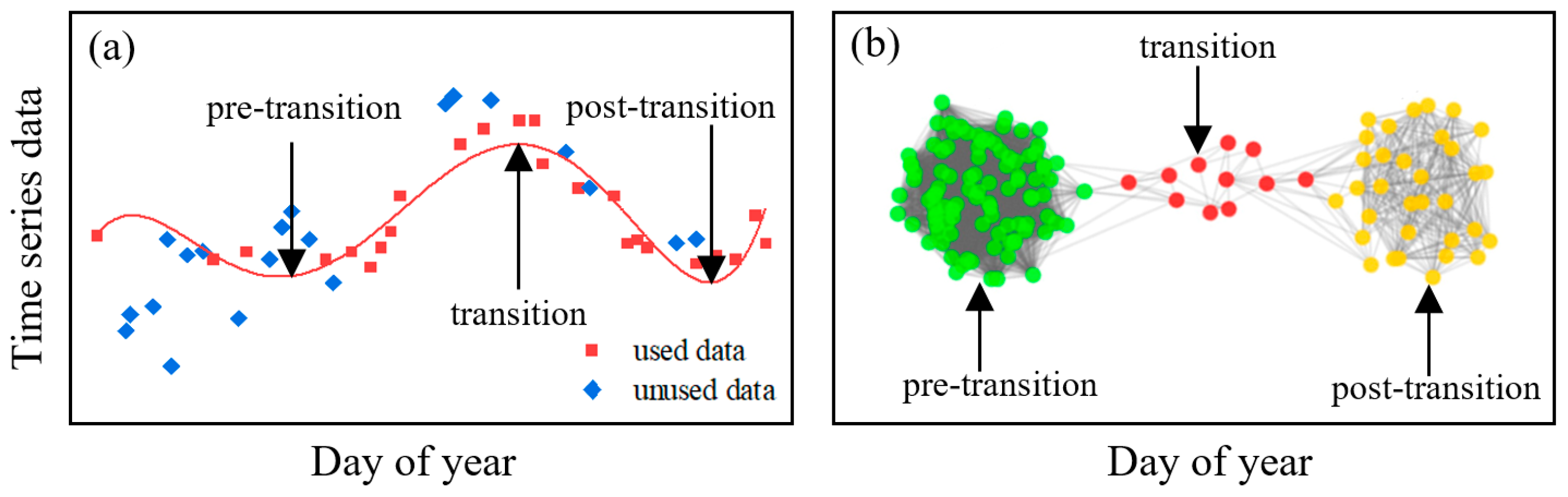
The satellite time-series data used to monitor vegetation phenological events are mostly curve-based (Figure 2a), which means the satellite time-series is presented as curves, and the features of the curves demonstrate the vegetation phenological stages [24]. These time-series are mainly VI-based, which may produce different phenological transition dates due to the lack of vegetation properties such as canopy pigment content, cell structure, and water content. Diao [16] recently represented time-series data as a series of nodes to take advantage of multiple spectral wavelengths (Figure 2b). Each node contains information of seven MODIS bands from visible to shortwave infrared, which can characterize several vegetation properties.
Taking advantage of the spectral signature nodes, the grouping-based model for peak coloration detection divided the satellite time-series into several groups according to the assumed phenological stages. For time-series data, we assumed that there were N nodes and k transition dates annually for the vegetation phenology (. Thus, the N nodes were then divided into k + 1 groups, and each group contained nodes. The total node number of the k + 1 groups is N:
The nodes within a group are more similar in terms of reflectance and spectral shape than those in different groups and are characterized by similarity. The similarity between the spectral signatures of nodes is defined as similarity distance (SD, d). Euclidean and cosine distances are frequently and commonly used metrics to measure “similarity distance”. However, the first one suffers from high sensitivity to magnitudes, whereas the second is less sensitive to magnitudes. The SD of a node pair is measured using cosine distance.
where A and B are vectors representing spectral signature nodes, and is the SD between A and B.
The total group distance (TGD, ) of the time-series is defined based on SD:
where and are the intra-group and inter-group SDs, respectively. The former is calculated as follows:
where is the intra-group SD of group i; and are two continuous nodes in group i to maintain the temporal order. The SD is calculated times for . Thus, SD is calculated times for all intra-group SDs. The inter-group SD is calculated as follows:
where is the inter-group SD of groups i and i + 1; is the end point in group i, and is the start point in group i + 1. The negative sign indicates that the inter-group SD should be large to minimize the TGD. In every , the SD is calculated once. The SD is then calculated times. The total calculation times of SD for a time-series are counted as follows:
where represents the total calculation times of SD, and is the total number of nodes of a time-series. is independent of the number of divided groups (k + 1). This interpretation indicates that the TGD is only influenced by the similarity of intra- and inter-group nodes, and insensitive to the number of groups. This interpretation may have advantages of not involving a pre-defined number of transition stages, whereas previous studies have needed an empirical number of transition dates [2,16].
2.4. Determination of Peak Coloration Periods
The best fall peak coloration transition dates correspond to the minimum TGD of a time-series. According to in-situ measurements of fall phenology at Harvard Forest, the mean peak coloration period is within the day of year (DOY) 270 to 310; the mean start date of peak coloration is before DOY 290 and the mean end is later than DOY 290 [16]. The fall field observations were typically conducted from DOY 240 to 330 at Harvard Forest. Thus, only the MODIS data during DOY 240 to 330 were used to form the time-series.
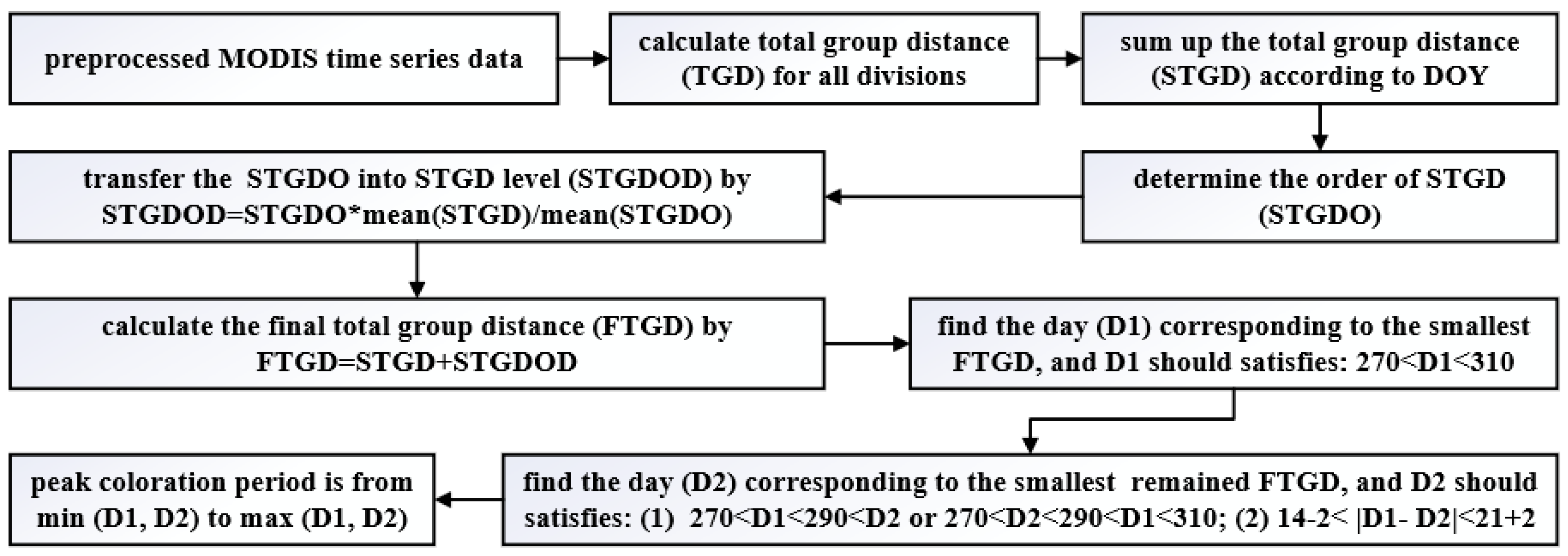
In practice, the MODIS time-series were divided into three groups by the start and end dates of peak coloration. The start date was set from DOY 240 to 329, and the end date was set from DOY 241 to 330 to explore all cases. After calculations of all cases of the start and end dates, the TGD were summed according to the DOY and the summed TGD (STGD) was ordered. The order of STGD (STGDO) was then transformed into distance-level (STGDOD) by multiplying the ratio of mean STGD and STGDO. The final TGD (FTGD) was the sum of the STGD and STGDOD. The steps of determination of peak coloration periods are summarized in Figure 3.
The peak coloration periods were determined with some empirical constraints based on the FTGD: (1) according to field observations, the start and end peak coloration dates were assumed before and after DOY 290 within the range of DOY 270 to 310, respectively; and (2) the peak coloration period normally lasts for 2–3 weeks. Thus, the day (D1) corresponding to the smallest FTGD during DOY 270 to 310 was firstly determined as either the start or end peak coloration date. Then, another day (D2) satisfying the two constraints and corresponding to the smallest remaining FTGD was considered as the end or start peak coloration date.
3. Results
3.1. Optimal Spatial Scale using ETM+
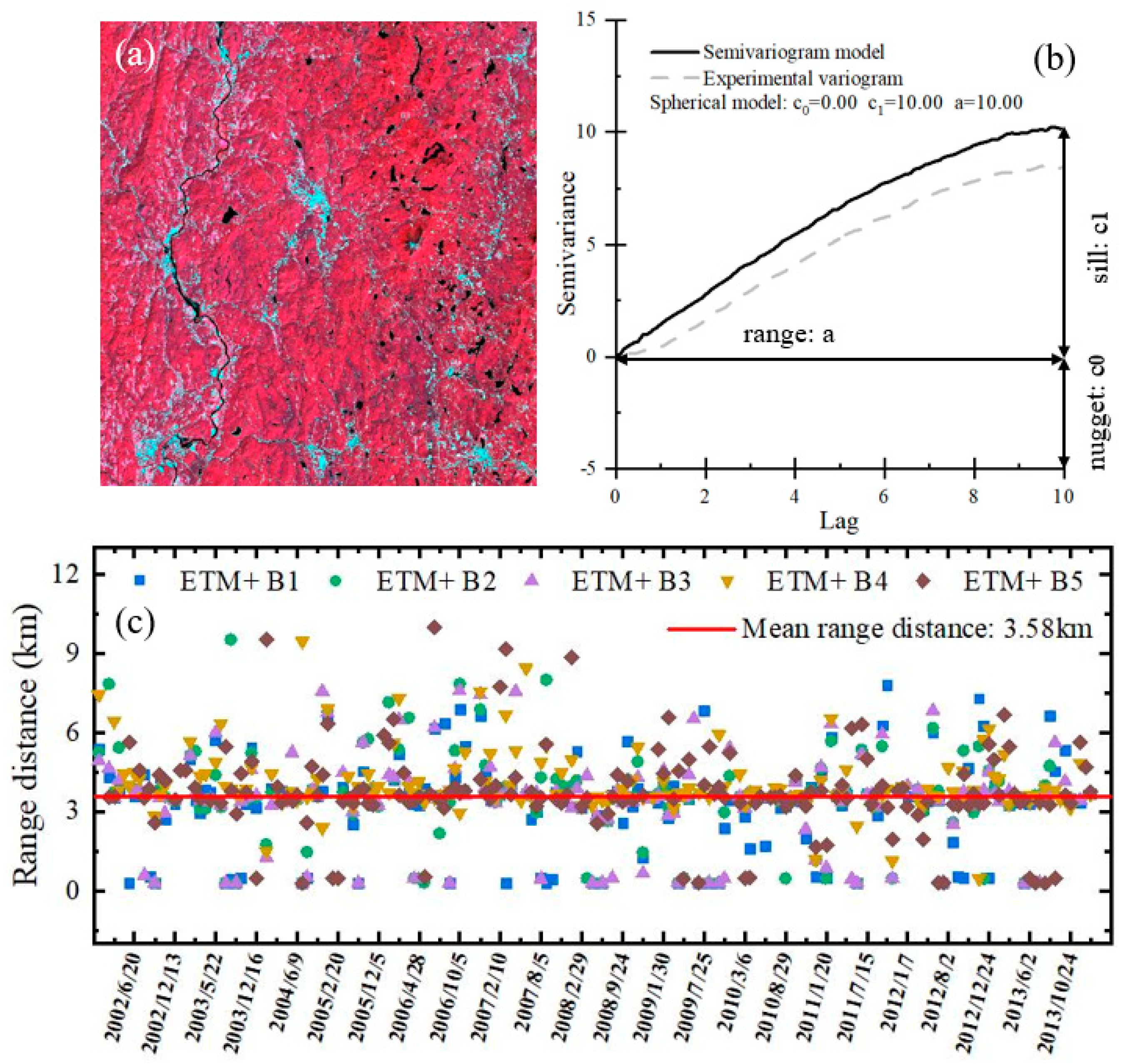
The optimal spatial scale at Harvard Forest was analyzed based on the semi-variance functions using ETM+ data (30 m) from 2002 to 2013. The optimal spatial scale for each ETM+ image is shown in Figure 4. The vegetation at Harvard Forest is dense, as can be seen in the false-color composite of the ETM+ image (Figure 4a). Figure 4b illustrates an example of a semi-variance function with a spherical model, and the range determines the optimal spatial scale. Figure 4c shows that the range distance of semi-variogram function is different for each image whilst similar for the five ETM+ bands, indicating that the semi-variance is not sensitive to bands. Although the range distance varies on different imaging days, the frequently occurring range distance is approximately 3500 m. This phenomenon may be attributed to the land surface that remains homogenous after atmospheric correction.
The mean range distance at Harvard Forest is approximately 3580 m from 2002 to 2013, which is about seven pixels of MODIS NBAR data (500 m). To avoid the potential influence of irregular spectral points and to reduce the uncertainty of geolocation, the mean value of MODIS NBAR data with a 7 × 7 window was adopted to represent the land surface. Without a window, the pixels influenced by absorbent aerosol, cloud shadow, and adjacent pixels may affect the performance of time-series models [16,18].
3.2. Optimal Temporal Scale using MODIS
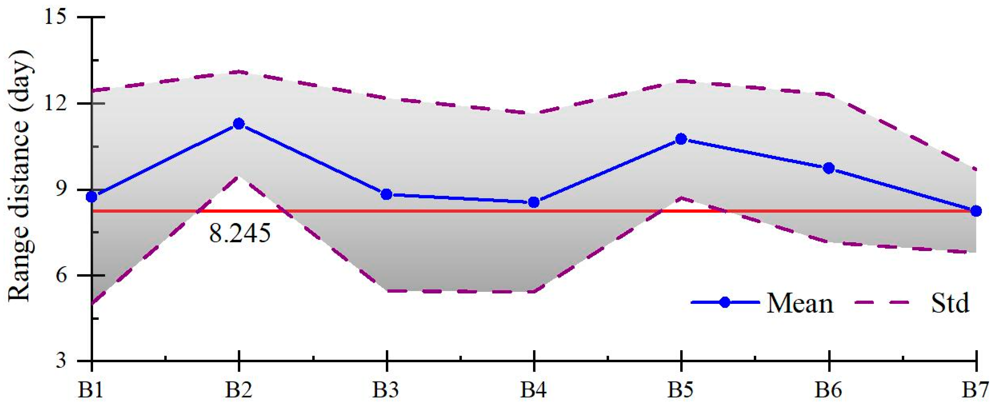
Irregular points in the time-series data affect the analysis and model performance [16]. Although the 16-day composite MODIS NBAR data were corrected for atmospheric influence, the pixels are occasionally unavoidably contaminated by absorbent aerosol, cloud shadow, or adjacent pixels [10,25]. To reduce the impacts of irregular nodes, the remote sensing time-series is usually averaged using moving windows and multiple window sizes are tested to yield the best results [16]. However, this strategy requires intense experiments and is occasionally time-consuming. Based on the semi-variance function, it is possible to determine the optimal window size for a time-series. Figure 5 shows the mean and standard deviation (Std) values of the temporal range distance of MODIS NBAR data at Harvard Forest. The temporal range distance slightly varies for different MODIS bands. The variations of B3 and B4 are large, possibly due to the fact that the short wavelength is most likely to be affected by atmospheric conditions [26].
The minimum of mean temporal range distance of MODIS NBAR data at Harvard Forest was approximately eight days. Since the window size is generally an odd number to determine the window center easily, the temporal window size was selected as seven days in this study, which is the same as the best window size for the network-based model in estimations of peak coloration transition dates at Harvard Forest [16].
3.3. Grouping-based Estimations of Peak Coloration Periods
After the optimal spatial and temporal scales are determined at Harvard Forest, the preprocessed MODIS NBAR data were first spatially averaged using a 7 × 7 window, and then temporally averaged with a 7-days moving window to form a reliable satellite time-series. Using the MODIS time-series data and grouping-based model, the fall peak coloration periods at Harvard Forest during 2002–2013 were estimated and listed in Table 2. The field-based peak coloration periods [16] are also included.
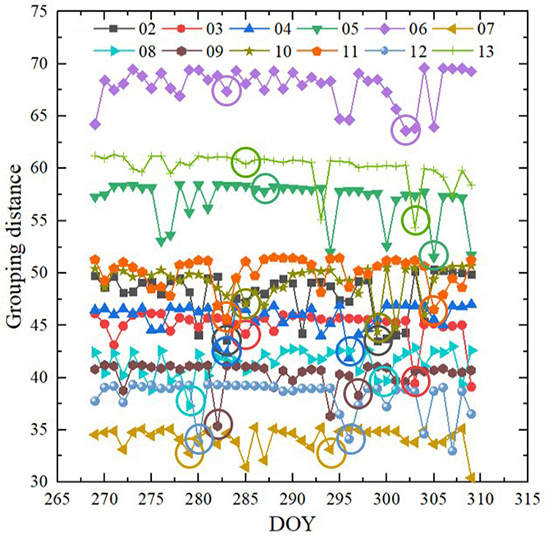
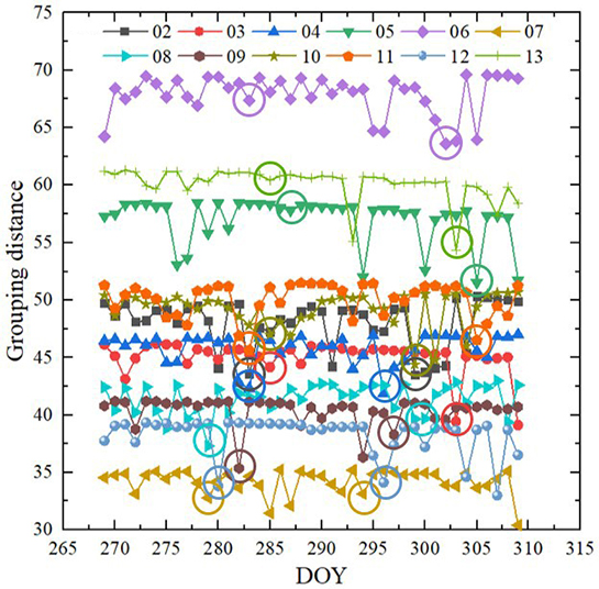
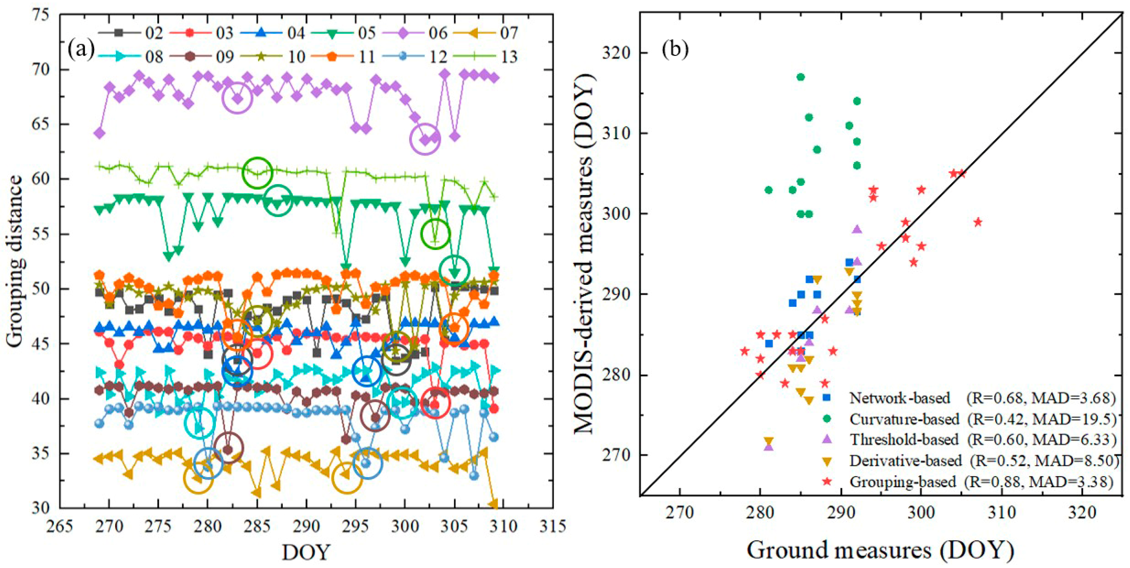
The mean peak coloration transition dates estimated by the grouping-based model are well consistent with the field observations at Harvard Forest, particularly for years from 2003 to 2005 and 2009 to 2012. The relationship between the grouping distance and the transition periods are displayed in Figure 6a, and comparison among the grouping-, curve-fitting- (threshold-, curve derivative-, and curvature change rate-based) and network-based models are shown in Figure 6b.
The start and end dates of peak coloration transition correspond to the small grouping-based distances. Although many local minimum grouping distances are observed, the date cannot be determined as the transition dates because the start and end dates should meet the empirical constraints (Section 2.4). Overall, the transition dates have small grouping-based distances and consistent with empirical knowledge.
Amongst the proposed grouping-based model and the four other phenological methods (threshold-, curve derivative-, curvature change rate-, and network-based models), the grouping-based model obtained the highest accuracy in calculations of the fall peak coloration dates compared with in-situ observations, with a correlation coefficient (R) of 0.88 and a mean absolute difference (MAD) of 3.38 days. The MAD between grouping-retrieved and field-observed peak coloration dates was smaller than the interval of field measurements (7 days). The grouping-based model considerably outperformed the conventional NDVI-based curve-fitting models and was comparable to the complex network-based model. The main advantages of the grouping-based model over the network-based model are that the former does not involve threshold selection and is much simpler. The comparisons of these models demonstrated that the grouping-based model has the potential to model fall peak coloration stages effectively.
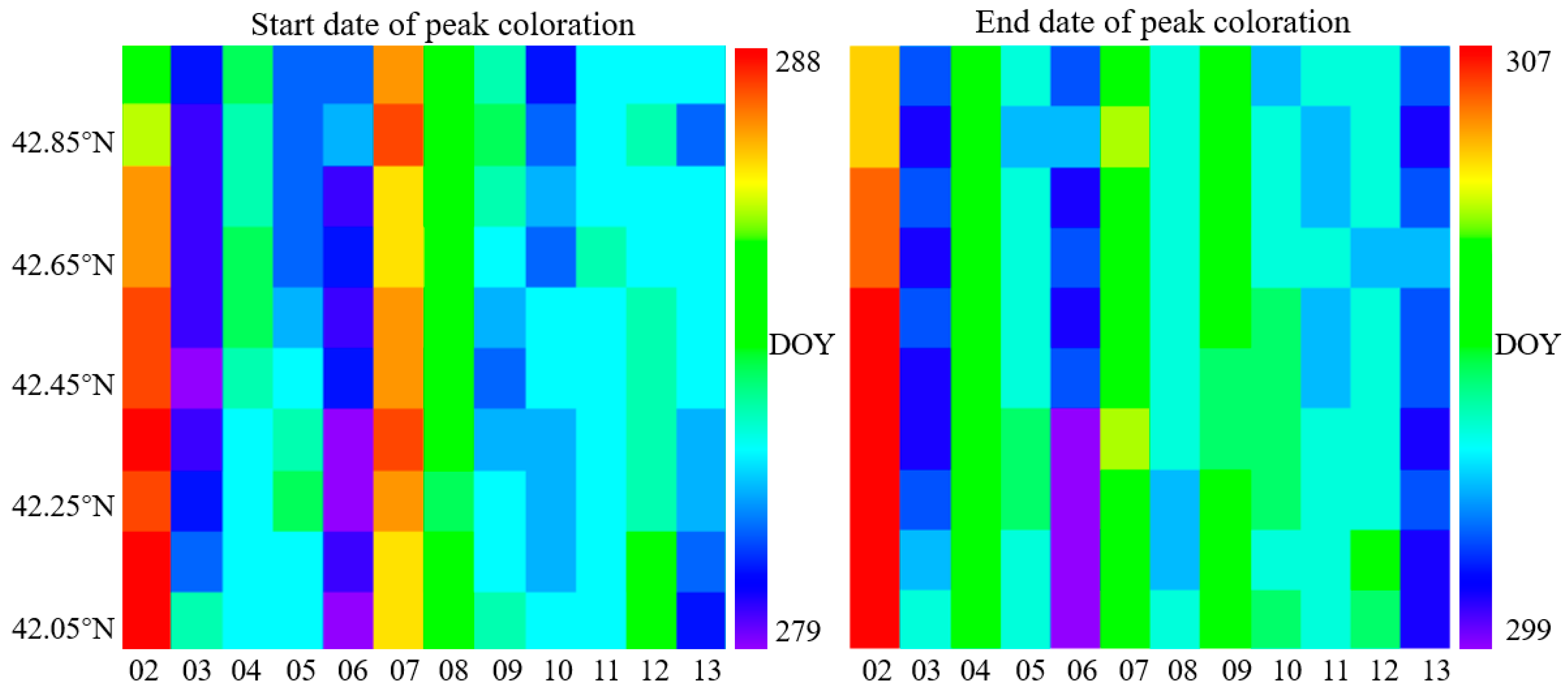
To visualize the spatial distributions of grouping-retrieved fall peak coloration dates from 2002–2013 at Harvard Forest, the fall peak coloration transition dates of a 1° × 1° region centered at Harvard Forest were estimated. Because the foliage phenological events are affected by temperature associated with latitude [24], the region was divided into ten small sections based on latitude with increments of 0.1° to analyze the latitude influence. The start and end dates of fall peak coloration periods from 2002–2013 are shown in Figure 7. Note that the biases between the field and the grouping-estimated dates were corrected for the 1° × 1° region.
In the 1° × 1° region, the transition dates are not obviously influenced by latitude (from the bottom to the top) possibly because the change in temperature in the small region is slight. However, the dates considerably vary for different years. Specifically, the start and end dates of peak coloration from 2002 to 2007 normally changed with increasing or decreasing trends. However, the start and end dates from 2007 to 2013 display a clear decreasing trend, indicating that the peak coloration periods were shifted to earlier dates.
4. Discussion
Satellite remote sensing has been widely used to monitor vegetation phenological events [16,21,24]. The grouping concept is introduced to remote sensing time-series in modeling the complex peak coloration processes. The overall performance of the grouping-based model, and its opportunities and limitations, are discussed below.
The grouping concept has been successfully used to deal with complex data flows [27,28,29]. In this study, the concurrent changes in spectral signatures along the phenological trajectory are reflected by the node similarity. Validated against field measurements at Harvard Forest, the retrieved peak coloration transition dates are well consistent with them. This indicates that the grouping-based similarity can differentiate the various vegetation phenological states, which cannot be adequately captured by curve fitting-based phenological approaches using a single VI [16]. The grouping concept provides a new perspective for the monitoring of vegetation phenological events.
Compared with the conventional VI-based phenological models, the grouping-based model can take advantage of multiple spectral signatures represented by the nodes. Each VI emphasizes a particular vegetation property, while the complex phenological process involves the concurrent changes of several vegetation properties, such as canopy pigment content, cell structure, and water content. These properties can be characterized by visible bands, near-infrared bands, and shortwave infrared bands, respectively [16]. MODIS bands from visible to shortwave infrared bands formed the nodes in the grouping-based model, indicating that the model can capture multiple vegetation properties. Compared with the novel network-based model, which also adopts the node concept, the grouping-based model is free from threshold selection, and thereby more flexible. The network-based model needs an appropriate threshold to construct a reasonable network graph [16]. Calculating the grouping similarity distance automatically without threshold selections can simplify the phenological model and make the model more robust.
To avoid the influence of irregular data in a time-series, the window sizes to process satellite data are based on empirical knowledge or tests of different sizes in previous studies [16]. In Diao [16], the spatial window size was set empirically as 6 × 6, and a series of window sizes ranging from one to seven days were tested to determine the best temporal window size. However, in this study, the spatial and temporal window sizes were determined using the semi-variance function [20], which can determine the optimal sampling size without empirical knowledge or extensive tests. Thus, the analysis of the remote sensing time-series is more reliable and accurate.
However, the proposed grouping-based time-series model still has several limitations. Firstly, the model was established based on the daily MODIS NBAR data, which might be affected by snow, clouds, and atmospheric effects [16]. More datasets, such as the AVHRR, MERIS, and VIIRS should be involved to create a more robust satellite remote sensing time-series [30]. Secondly, the methodical data processing steps for the determination of peak coloration periods need to be further explored and modified to avoid pre-defined assumptions. At present, the model needs to restrict the start and end dates within specific ranges, which might hinder the model’s global implementation. Finally, the grouping-based model is only validated using field observations at Harvard Forest, while validation is crucial in phenological studies based on remote sensing [11,16,31]. More phenological observations should be acquired to extensively evaluate the performance of the proposed model.
5. Conclusions
We have developed a new grouping-based time-series model for fall peak coloration period estimations, which has been successfully applied at Harvard Forest using MODIS data from 2002 to 2013. The model consists of three procedures: (1) preprocessing of MODIS data; (2) removal of spatial and temporal scale effects based on semi-variance function; and (3) determination of peak coloration transition dates using the grouping-based model.
The grouping-based model takes advantage of multiple MODIS spectral signatures and is free from threshold selections, and it outperforms the curving-fitting- and network-based methods when validated against field measurements at Harvard Forest. This study demonstrates that the grouping concept is useful in analyzing remote sensing time-series for the monitoring of complex vegetation phenological processes. We believe that the grouping concept has potential applicability to other phenological events and regions.
Overall, the grouping-based model showed good performance to support the monitoring of the fall plant phenology and could complement the current time-series models. In the near future, we will conduct investigations on the determination steps of transition dates for peak coloration estimation to free the model from empirical knowledge and apply the model to other regions to explore its feasibility.
Author Contributions
The project was coordinated by Q.Z. who took the lead in writing this article. L.T. and J.L. outlined the research topic. Q.Z. and X.S. organized the research collaboration, reviewed the manuscript, and contributed to the writing. X.S. and W.L. contributed to the writing and editing of the manuscript. All authors have read and agreed to the published version of the manuscript.
Funding
This research was funded by the National Key R&D Program of China (2018YFB0504900, 2018YFB0504904, and 2016YFC0200900) and the National Natural Science Foundation of China (41571344 and 41701379).
Acknowledgments
The authors would like to thank the LP DAAC for providing the MODIS data (https://lpdaac.usgs.gov/) and John O’Keefe for making the phenological data at Harvard Forest available (http://harvardforest.fas.harvard.edu).
Conflicts of Interest
The authors declare no conflict of interest.
References
- Kimball, J.S.; McDonald, K.C.; Running, S.W.; Frolking, S.E. Satellite radar remote sensing of seasonal growing seasons for boreal and subalpine evergreen forests. Remote Sens. Environ. 2004, 90, 243–258. [Google Scholar] [CrossRef]
- Chen, M.; Melaas, E.K.; Gray, J.M.; Friedl, M.A.; Richardson, A.D. A new seasonal-deciduous spring phenology submodel in the Community Land Model 4.5: Impacts on carbon and water cycling under future climate scenarios. Glob. Chang. Biol. 2016, 22, 3675–3688. [Google Scholar] [CrossRef] [PubMed] [Green Version]
- Visser, M.E. Phenology: Interactions of climate change and species. Nature 2016, 535, 236–237. [Google Scholar] [CrossRef] [PubMed]
- Clark, J.S.; Melillo, J.; Mohan, J.; Salk, C. The seasonal timing of warming that controls onset of the growing season. Glob. Chang. Biol. 2014, 20, 1136–1145. [Google Scholar] [CrossRef] [PubMed]
- Xie, Y.; Wang, X.; Wilson, A.M.; Silander, J.A. Predicting autumn phenology: How deciduous tree species respond to weather stressors. Agric. For. Meteorol. 2018, 250, 127–137. [Google Scholar] [CrossRef]
- Garonna, I.; de Jong, R.; de Wit, A.J.W.; Mücher, C.A.; Schmid, B.; Schaepman, M.E. Strong contribution of autumn phenology to changes in satellite-derived growing season length estimates across Europe (1982–2011). Glob. Chang. Biol. 2014, 20, 3457–3470. [Google Scholar] [CrossRef]
- Jeong, S.J.; Medvigy, D. Macroscale prediction of autumn leaf coloration throughout the continental United States. Glob. Ecol. Biogeogr. 2014, 23, 1245–1254. [Google Scholar] [CrossRef]
- Zhou, Q.; Tian, L.; Wai, O.W.H.; Li, J.; Sun, Z.; Li, W. Impacts of insufficient observations on the monitoring of short- and long-term suspended solids variations in highly dynamic waters, and implications for an optimal observation strategy. Remote Sens. 2018, 10, 345. [Google Scholar] [CrossRef] [Green Version]
- Liang, L.; Schwartz, M.D.; Fei, S. Validating satellite phenology through intensive ground observation and landscape scaling in a mixed seasonal forest. Remote Sens. Environ. 2011, 115, 143–157. [Google Scholar] [CrossRef]
- Sakamoto, T.; Yokozawa, M.; Toritani, H.; Shibayama, M.; Ishitsuka, N.; Ohno, H. A crop phenology detection method using time-series MODIS data. Remote Sens. Environ. 2005, 96, 366–374. [Google Scholar] [CrossRef]
- Zhang, X.; Friedl, M.A.; Schaaf, C.B.; Strahler, A.H.; Hodges, J.C.F.; Gao, F.; Reed, B.C.; Huete, A. Monitoring vegetation phenology using MODIS. Remote Sens. Environ. 2003, 84, 471–475. [Google Scholar] [CrossRef]
- Reed, B.C.; Brown, J.F.; VanderZee, D.; Loveland, T.R.; Merchant, J.W.; Ohlen, D.O. Measuring phenological variability from satellite imagery. J. Veg. Sci. 1994, 5, 703–714. [Google Scholar] [CrossRef]
- Dragoni, D.; Rahman, A.F. Trends in fall phenology across the deciduous forests of the Eastern USA. Agric. For. Meteorol. 2012, 157, 96–105. [Google Scholar] [CrossRef]
- White, M.A.; Thornton, P.E.; Running, S.W. A continental phenology model for monitoring vegetation responses to interannual climatic variability. Glob. Biogeochem. Cycles 1997, 11, 217–234. [Google Scholar] [CrossRef]
- Toda, M.; Richardson, A.D. Estimation of plant area index and phenological transition dates from digital repeat photography and radiometric approaches in a hardwood forest in the Northeastern United States. Agric. For. Meteorol. 2018, 249, 457–466. [Google Scholar] [CrossRef]
- Diao, C. Complex network-based time series remote sensing model in monitoring the fall foliage transition date for peak coloration. Remote Sens. Environ. 2019, 229, 179–192. [Google Scholar] [CrossRef]
- Zhou, Q.; Tian, L.; Li, J.; Song, Q.; Li, W. Radiometric cross-calibration of Tiangong-2 MWI visible/NIR channels over aquatic environments using MODIS. Remote Sens. 2018, 10, 1803. [Google Scholar] [CrossRef] [Green Version]
- Li, J.; Chen, X.; Tian, L.; Huang, J.; Feng, L. Improved capabilities of the Chinese high-resolution remote sensing satellite GF-1 for monitoring suspended particulate matter (SPM) in inland waters: Radiometric and spatial considerations. ISPRS J. Photogramm. Remote Sens. 2015, 106, 145–156. [Google Scholar] [CrossRef]
- Woodcock, C.E.; Strahler, A.H. The factor of scale in remote sensing. Remote Sens. Environ. 1987, 21, 311–332. [Google Scholar] [CrossRef]
- Atkinson, P.M.; Curran, P.J. Defining an Optimal Size of Support for Remote Sensing Investigations. IEEE Trans. Geosci. Remote Sens. 1995, 33, 768–776. [Google Scholar] [CrossRef]
- Ahl, D.E.; Gower, S.T.; Burrows, S.N.; Shabanov, N.V.; Myneni, R.B.; Knyazikhin, Y. Monitoring spring canopy phenology of a deciduous broadleaf forest using MODIS. Remote Sens. Environ. 2006, 104, 88–95. [Google Scholar] [CrossRef] [Green Version]
- Brocca, L.; Tullo, T.; Melone, F.; Moramarco, T.; Morbidelli, R. Catchment scale soil moisture spatial-temporal variability. J. Hydrol. 2012, 422–423, 63–75. [Google Scholar] [CrossRef]
- Gorelick, N.; Hancher, M.; Dixon, M.; Ilyushchenko, S.; Thau, D.; Moore, R. Google Earth Engine: Planetary-scale geospatial analysis for everyone. Remote Sens. Environ. 2017, 202, 18–27. [Google Scholar] [CrossRef]
- Zhang, X.; Goldberg, M.D.; Yu, Y. Prototype for monitoring and forecasting fall foliage coloration in real time from satellite data. Agric. For. Meteorol. 2012, 158–159, 21–29. [Google Scholar] [CrossRef] [Green Version]
- Delbart, N.; Kergoat, L.; Le Toan, T.; Lhermitte, J.; Picard, G. Determination of phenological dates in boreal regions using normalized difference water index. Remote Sens. Environ. 2005, 97, 26–38. [Google Scholar] [CrossRef] [Green Version]
- Yang, A.; Zhong, B.; Lv, W.; Wu, S.; Liu, Q. Cross-calibration of GF-1/WFV over a desert site using Landsat-8/OLI imagery and ZY-3/TLC data. Remote Sens. 2015, 7, 10763–10787. [Google Scholar] [CrossRef] [Green Version]
- Xu, S.; Liu, Y.; Zhang, W. Grouping-based discontinuous reception for massive narrowband internet of things systems. IEEE Internet Things J. 2018, 5, 1561–1571. [Google Scholar] [CrossRef]
- Mao, J.; Wang, T.; Jin, C.; Zhou, A. Feature grouping-based outlier detection upon streaming trajectories. IEEE Trans. Knowl. Data Eng. 2017, 29, 2696–2709. [Google Scholar] [CrossRef]
- Lee, B.; Choi, J.; Seol, J.Y.; Love, D.J.; Shim, B. Antenna Grouping Based Feedback Compression for FDD-Based Massive MIMO Systems. IEEE Trans. Commun. 2015, 63, 3261–3274. [Google Scholar] [CrossRef] [Green Version]
- Pouliot, D.; Latifovic, R.; Fernandes, R.; Olthof, I. Evaluation of compositing period and AVHRR and MERIS combination for improvement of spring phenology detection in deciduous forests. Remote Sens. Environ. 2011, 115, 158–166. [Google Scholar] [CrossRef]
- Schwartz, M.D.; Reed, B.C. Surface phenology and satellite sensor-derived onset of greenness: An initial comparison. Int. J. Remote Sens. 1999, 20, 3451–3457. [Google Scholar] [CrossRef]
Figure 1.
The preprocessing steps of satellite images.

Figure 2.
Two ways to handle time-series data: (a) as curves according to Sakamoto et al. [10] and (b) as points according to Diao [16].

Figure 3.
Data processing steps to determine the peak coloration periods by the grouping-based time-series approach.
Figure 3.
Data processing steps to determine the peak coloration periods by the grouping-based time-series approach.

Figure 4.
(a) False-color composite of an ETM+ image on 8 September 2002 at Harvard Forest; (b) example of a semi-variance function [20]; and (c) the spatial range distances of five Enhanced Thematic Mapper Plus (ETM+) bands from 2002 to 2013.
Figure 4.
(a) False-color composite of an ETM+ image on 8 September 2002 at Harvard Forest; (b) example of a semi-variance function [20]; and (c) the spatial range distances of five Enhanced Thematic Mapper Plus (ETM+) bands from 2002 to 2013.

Figure 5.
Mean and Std temporal range distance of seven MODIS bands using MODIS Nadir Bidirectional reflectance distribution function Adjusted Reflectance (NBAR) data at Harvard Forest from 2002 to 2013.
Figure 5.
Mean and Std temporal range distance of seven MODIS bands using MODIS Nadir Bidirectional reflectance distribution function Adjusted Reflectance (NBAR) data at Harvard Forest from 2002 to 2013.

Figure 6.
(a) Estimated start and end dates (circles) for peak coloration using the grouping-based time-series analysis from 2002 to 2013 at Harvard Forest; (b) comparisons of the grouping-, three conventional curve-fitting-, and complex network-based models in estimating coloration transition dates from 2002 to 2013 at Harvard Forest. The results of curve-fitting- and network-based methods are obtained from Diao [16].

Figure 7.
The 1° × 1° region centered at Harvard Forest was divided into ten small sections based on latitude with increments of 0.1°. The start and end dates of peak coloration were represented during the 12 years of the study period.
Figure 7.
The 1° × 1° region centered at Harvard Forest was divided into ten small sections based on latitude with increments of 0.1°. The start and end dates of peak coloration were represented during the 12 years of the study period.


Table 1.
Information and roles of Moderate Resolution Imaging Spectroradiometer (MODIS) datasets.
| Data | Spatial Resolution | Temporal Resolution | Roles |
|---|---|---|---|
| NBAR | 500 m | daily, 16-day composite | estimate the peak coloration dates |
| BAQ | 500 m | daily, 16-day composite | locate the pixels covered by snow |
| LST | 1000 m | daily, 16-day composite | locate the winter periods |
| LCT | 500 m | yearly, 16-day composite | determine the land cover types |
Table 2.
The mean field-based and MODIS-estimated transition dates for fall peak coloration at Harvard Forest from 2002 to 2013. The mean field-based results are adopted from Diao [16].
Table 2.
The mean field-based and MODIS-estimated transition dates for fall peak coloration at Harvard Forest from 2002 to 2013. The mean field-based results are adopted from Diao [16].
| Year | Field | MODIS | Year | Field | MODIS | Year | Field | MODIS |
|---|---|---|---|---|---|---|---|---|
| 02 | [289, 307] | [283, 299] | 06 | [278, 294] | [283, 302] | 10 | [282, 298] | [285, 299] |
| 03 | [284, 300] | [285, 303] | 07 | [288, 299] | [279, 294] | 11 | [284, 304] | [283, 305] |
| 04 | [285, 300] | [283, 296] | 08 | [283, 298] | [279, 299] | 12 | [280, 295] | [280, 296] |
| 05 | [288, 305] | [287, 305] | 09 | [280, 298] | [282, 297] | 13 | [280, 294] | [285, 302] |
© 2020 by the authors. Licensee MDPI, Basel, Switzerland. This article is an open access article distributed under the terms and conditions of the Creative Commons Attribution (CC BY) license (http://creativecommons.org/licenses/by/4.0/).
Share and Cite
MDPI and ACS Style
Zhou, Q.; Sun, X.; Tian, L.; Li, J.; Li, W. Grouping-Based Time-Series Model for Monitoring of Fall Peak Coloration Dates Using Satellite Remote Sensing Data. Remote Sens. 2020, 12, 274. https://0-doi-org.brum.beds.ac.uk/10.3390/rs12020274
AMA Style
Zhou Q, Sun X, Tian L, Li J, Li W. Grouping-Based Time-Series Model for Monitoring of Fall Peak Coloration Dates Using Satellite Remote Sensing Data. Remote Sensing. 2020; 12(2):274. https://0-doi-org.brum.beds.ac.uk/10.3390/rs12020274
Chicago/Turabian StyleZhou, Qu, Xianghan Sun, Liqiao Tian, Jian Li, and Wenkai Li. 2020. "Grouping-Based Time-Series Model for Monitoring of Fall Peak Coloration Dates Using Satellite Remote Sensing Data" Remote Sensing 12, no. 2: 274. https://0-doi-org.brum.beds.ac.uk/10.3390/rs12020274
Note that from the first issue of 2016, this journal uses article numbers instead of page numbers. See further details here.