Do Game Data Generalize Well for Remote Sensing Image Segmentation?


1
Department of Computational Medicine and Bioinformatics, University of Michigan, Ann Arbor, MI 48109, USA
2
Image Processing Center, School of Astronautics, Beihang University, Beijing 100191, China
3
Beijing Key Laboratory of Digital Media, Beihang University, Beijing 100191, China
4
State Key Laboratory of Virtual Reality Technology and Systems, School of Astronautics, Beihang University, Beijing 100191, China
5
Department of Biological Systems Engineering, University of Wisconsin-Madison, Madison, WI 53706, USA
*
Author to whom correspondence should be addressed.
†
These authors are co-first authors as they contributed equally to this work.
Remote Sens. 2020, 12(2), 275; https://0-doi-org.brum.beds.ac.uk/10.3390/rs12020275
Submission received: 10 December 2019
/
Revised: 8 January 2020
/
Accepted: 10 January 2020
/
Published: 14 January 2020
(This article belongs to the Special Issue Computational Intelligence and Advanced Learning Techniques in Remote Sensing)
Abstract
:Despite the recent progress in deep learning and remote sensing image interpretation, the adaption of a deep learning model between different sources of remote sensing data still remains a challenge. This paper investigates an interesting question: do synthetic data generalize well for remote sensing image applications? To answer this question, we take the building segmentation as an example by training a deep learning model on the city map of a well-known video game “Grand Theft Auto V” and then adapting the model to real-world remote sensing images. We propose a generative adversarial training based segmentation framework to improve the adaptability of the segmentation model. Our model consists of a CycleGAN model and a ResNet based segmentation network, where the former one is a well-known image-to-image translation framework which learns a mapping of the image from the game domain to the remote sensing domain; and the latter one learns to predict pixel-wise building masks based on the transformed data. All models in our method can be trained in an end-to-end fashion. The segmentation model can be trained without using any additional ground truth reference of the real-world images. Experimental results on a public building segmentation dataset suggest the effectiveness of our adaptation method. Our method shows superiority over other state-of-the-art semantic segmentation methods, for example, Deeplab-v3 and UNet. Another advantage of our method is that by introducing semantic information to the image-to-image translation framework, the image style conversion can be further improved.
1. Introduction
The remote sensing technology opens a door for us to a better understanding of our planet, changing all walks of our life with very broad applications, including disaster relief, land monitoring, city planning and so forth. With the rapid advances in imaging sensor technology, the modality of the remote sensing data is becoming more and more diversified. People now can easily acquire and access to up-to-date remote sensing images from a variety of imaging platforms (e.g., airborne, spaceborne) with a wide spectral range (from multi-spectrum to hyper-spectrum) at multiple spatial resolutions (from centimeters to kilometers).
Recently, deep learning technology [1,2] has drawn great attention in a variety of research fields. The deep Convolutional Neural Networks (CNNs), as one of the deep neural architectures, have greatly promoted the progress of remote sensing technology [3,4,5,6,7]. Despite its great success in automatic remote sensing image analysis, the adaption of a deep learning model between different sources of remote sensing data still remains a challenge. On one hand, most of the previous methods of this field are designed and tuned based on images of specific resolution or motility. When these methods are applied across different platforms (e.g., the remote sensing images with different modality or image resolution), their performance will be deeply affected. On the other hand, as deep neural networks’ capacity is growing rapidly, the training of a deep learning model requires a huge amount of training data with high-quality annotations, but the manual labeling of these data is time-consuming, expensive and may heavily rely on domain knowledge.
Arguably, improving the adaptability of a model between the different sources of images can be essentially considered as a visual domain adaptation problem [8,9,10]. The mechanism behind the degradation lies in the none independent and identically distributed data between the training and deployment, that is, the “domain shift” [8,11] between different sources. Since the training of most of the deep CNN models can be essentially viewed as a maximum likelihood estimation process under the “independent and identically distribution” assumption [2], once the data distribution has changed after training, the performance can be deeply affected. An important idea for tackling this problem is to learn a mapping/transformation between the two groups of data (e.g., the training data and the testing data) so that they will have, in principle, the same distribution.
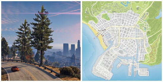
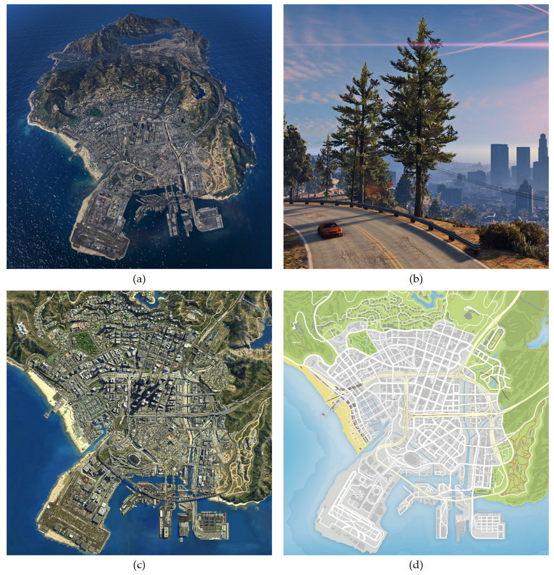
In the computer vision field, efforts have been made to generalize a model trained on the rendered images [12,13] (e.g., computer games) to real-world computer vision tasks and have obtained promising results [14,15,16,17]. In recent video games, for example, Grand Theft Auto (https://www.rockstargames.com/), Hitman (https://hitman.com/) and Watch Dogs (https://www.ubisoft.com/en-us/game/watch-dogs/), to improve a player’s immersion, the game developers have made great efforts to feature sophisticated and highly realistic game environment. The realism of these games not only lies in the high reality of material appearance, illumination but also in the content of the environment: the ground objects, structure layout, vehicles and non-player characters [13]. In addition to realism, the size of the game maps are also growing explosively and are made more and more sophisticated. For example, in a well-known game “Grand Theft Auto V (GTA-V)” (https://www.rockstargames.com/V/), the Los Santos, a fictional city featured in the game’s open world, covers an area of over 100 km with unprecedented details. Reviewers praised its design and similarity to Los Angeles. Figure 1 shows a part of its official map and a frame rendered by the game engine.
In this paper, we investigate an interesting question: do synthetic data generalize well for remote sensing applications? To answer this question, we train a remote sensing image segmentation model on the city map of the well-known video game GTA-V and then adapting it to real-world remote sensing application scenarios. Due to the “domain shift” between the game and the real world, we cannot simply apply the models trained on game data to real-world applications since it may lead to a large generalization error. A general practice to tackle this problem is the “neural style transfer” that is, to transform a game image by using a deep neural network so that the transformed image shares a similar style with a real-world one while keeping its original image contents unchanged [18,19,20,21]. The Fully Convolutional Adaptation Network (FCAN) [14] is a representative of this group of the methods. The FCAN aims to improve the street-view image segmentation across different domains. By transforming the game data to the style of urban street scenes based on neural style transfer, it narrows the domain gap and improves the segmentation performance. More recently, Generative Adversarial Networks (GAN) [22,23] has greatly promoted the progress of image translation [22,24,25,26]. Zhu et al. proposed a method called CycleGAN [26], which has achieved impressive results in a variety of image-to-image translation tasks. Owing to the “cycle consistency loss” they introduced, people are now able to obtain realistic transformations between the two domains even without the instruction of paired training data. CycleGAN has then been applied to improve visual domain adaptation tasks [15,27].
In this paper, we choose a fundamental application in remote sensing image interpretation, that is, the building segmentation, as an example by training a deep learning model on the city map of the game GTA-V and then adapting our model to real-world remote sensing images. We build our dataset based on the GTA-V official game maps. Different to any previous methods [14,15,16,17] and any previous image segmentation dataset [12,13] that focuses on the game images generated from the “first-person perspective” or from the “street view”, our dataset is built from an “aerial view” of the game world, resulting more abundant ground features and spatial relationship of different ground objects.
We further proposed a generative adversarial training based method, called “CycleGAN based Fully Convolutional Networks (CGFCN)’,on top of the CycleGAN [26], to improve the adaptability of a deep CNN model to different sources of remote sensing data. Our model consists of a CycleGAN model [26] and a deep Fully Convolutional Networks (FCN) [28,29] based segmentation model, where the former one learns to transforms the style of an image from the “game domain” to the “remote sensing domain” and the latter one learns to predict pixel-wise building masks. The two models can be trained jointly without requiring any additional ground truth reference of the real-world images. An overview of the proposed method is shown in Figure 2.
Different to previous methods like FCAN [14], where the image transformation model and the segmentation model are trained separately, our model can be jointly optimized in a unified training framework, which leads to additional performance gains. Experimental results on Massachusetts Buildings [30], a well-known building segmentation dataset, suggest the effectiveness of our adaptation method. Our method shows superiority over some other state-of-the-art semantic segmentation methods, for example, Deeplab-v3 [29] and UNet [31]. In addition, by introducing semantic information to the image-to-image translation framework, the image style conversion of the CycleGAN can be further improved by using our method. The contributions of our paper can be summarized as follows:
- We investigate an interesting question: do game data generalize well for remote sensing image segmentation? This is a brand-new question for the remote sensing community and it may have great application significance. To answer this, we study the domain adaptation ability of a deep learning based segmentation methods by training our model based on the rendered in-game data and then apply it to real-world remote sensing tasks. We propose a new method called CycleGAN to tackle the domain shift problem by first transferring the game data to real-world fashion and then producing pixel-wise segmentation output. In fact, the innovation of our paper is not limited to a certain algorithm - the significance of our work also lies in our investigation of a brand-new task in remote sensing and a feasible solution. To our best knowledge, this problem was rarely studied before and we haven’t seen any similar solution proposed in the remote sensing community.
- We introduce a synthetic dataset for building segmentation based on the well-known video game GTA-V. Different to the previous datasets [12,13] that focuses on rendering street-view images from the “first-person perspective”, we build our dataset from the “aerial perspective” of the city. To our best knowledge, this is the first synthetic dataset that focuses on aerial view image segmentation tasks and this is also the first game-based dataset for remote sensing applications. We will make our dataset publicly available at https://github.com/jiupinjia/gtav-sattellite-imagery-dataset.
2. Materials and Methods
In this section, we will first give a brief review of some related methods, including the fully convolutional networks [28], vanilla GAN [22] and the CycleGAN [26]. Then, we will give a detailed introduction of the proposed CGFCN. Finally, we will introduce our experimental datasets and evaluation metrics.
2.1. Fully Convolutional Networks
In recent years, deep CNNs [32,33,34,35] have greatly promoted the research of image processing and computer vision, including object detection [36,37,38,39,40,41], semantic segmentation [28,42,43], image captioning [44,45,46], image super-resolution [47,48,49], and so forth. A CNN consists of multiple convolutional and down-sampling layers, learning high-level image abstraction of the data in a layer-wise fashion with better discriminative ability and robustness. Compared with the traditional methods where the features are manually designed, the features of a deep CNN can be automatically learned through an end-to-end learning framework.
The fast development of deep CNNs gave birth to a new technique called Fully Convolutional Networks (FCN) [28,29]. An FCN is a network architecture that is specially designed to predict two-dimensional structured outputs. Compared to a standard CNN that only accepts images of a fixed size and produces one-dimensional vectorized outputs, an FCN can accept arbitrary-sized inputs and produce two-dimensional outputs accordingly, which greatly improves the flexibility of data processing. The FCN thus proves to be much more effective than the traditional CNNs in many computer vision tasks. Similar to a standard CNN, an FCN consists of a series of layers, including convolutional layers, activation layers and pooling layer, stacked repeatedly in a certain order. The difference between an FCN and a CNN lies in their output layer—a CNN uses a fully connected layer at its output end, while an FCN replaces it with a 1 × 1 convolutional layer. When we train an FCN, a loss function needs to be specifically designed according to our tasks (e.g., classification, regression, etc.). In a pixel-to-pixel translation task, the loss of the whole two-dimensional output can be written as the average of the losses of every pixel in its output map.
2.2. Generative Adversarial Networks (GAN)
Generative Adversarial Network (GAN) was originally proposed by A. Goodfellow et al. in 2014 [22]. It has then received increasing attention and achieved impressive results in a variety of image processing and computer vision tasks, for example, image generation [50,51,52,53], image-to-image translation [26,54,55], object detection [56,57,58], image super-resolution [49,59,60], and so forth.
The essence of a GAN is the idea of “adversarial training,” where two networks, a generator G and a discriminator D, are trained to contest with each other in a minimax two-player game and forces the generated data to be, in principle, indistinguishable from real ones. In this framework, the generator aims to learn a mapping from a input noise space to a data distribution of the target. The discriminator, on one hand, is trained to discriminate between the samples from the true data distribution and those generated , on the other hand, feeds its output back to G to further make the generated data indistinguishable from real ones. The training of a GAN can be considered as solving the following minimax problem:
where x and z represent a true data point and an input random noise. The above problem can be well-solved by iteratively updating D and G: that is, by first fixing G and updating D to maximize , and then fixing D and updating G to minimize . As the adversarial training progresses, the D will have more powerful discriminative ability and thus the images generated by the G will become more and more realistic. As is suggested by I. Goodfellow et al. [22], instead of updating G to minimize , in practice, many researchers choose to maximize . This is because in the early stage of learning, tends to saturate. This revision on objective provides much stronger gradients.
2.3. CycleGAN for Image-to-Image Translation
Suppose X represents a source domain (e.g., the game maps), Y represents a target domain (e.g., the real-world remote sensing images) and and are their training samples. In a GAN-based image-to-image translation task [26,54], we aim to learn a mapping G: by using an adversarial loss, such that the generated images is indistinguishable from those real images from the distribution Y. In this case, the above random noise vector z in the vanilla GAN will be replaced by an input image x. In addition, the generator G and the discriminator D are usually constructed based on deep CNNs [51]. Similar to the vanilla GAN [22], the G and D are also trained to compete with each other. Their objective function can be rewritten as follows:
where x and y represent two images from the domain X and domain Y. and are their data distributions.
In 2017, Zhu et al. proposed CycleGAN [26] for solving the unpaired image-to-image translation problem. The main innovation of the CycleGAN is the introduction of the cycle “consistency loss” in the adversarial training framework. CycleGAN breaks the limits of previous GAN based image translation methods, in which their models need to be trained by pair-wise images between the source and target domains. Since no pair-wise training data is provided, they deal with this problem with an inverse mapping F: and enforce (and vice versa).
A CycleGAN consists of four networks: two generative networks , and two discriminative networks , . To transform the style of an image to the domain Y, a straight forward implementation would be training the to learn a mapping from X to Y so that to fool the to make it fail to tell which domain they belong to. The objective function for training the and can thus be written as follows:
where maps the data from domain X to domain Y and is trained to classify whether the transformed data is real or fake. Similarly, can also be trained to learn to map the data from Y to X and is trained to classify it. The objective function for the training of and can thus be written as .
However, since the mapping is highly under-constrained, with large enough model capacity, the networks and can map the same set of input images to any random locations in the target domain if no pair-wise training supervision is provided [26], thus may fail to learn image correspondence between the two domains. To this end, the CycleGAN introduces a cycle consistency loss that further enforces the transformed image to be mapped back to itself in the original domain: . The cycle consistency loss is defined as follows:
where represents the pixel-wise loss (sum of absolute difference of each pixel between the input and the back-projected output). The CycleGAN uses pixel-wise loss rather the loss since the former one encourages less blurring effect.
2.4. CGFCN
We build our model based on the CycleGAN. Our model consists of five networks: , , , and F, where the (, , , ) correspond to a CycleGAN, and the F is a standard FCN based image segmentation network. An overview of the proposed method is shown in Figure 2.
The goals of the proposed CGFCN is twofold. On one hand, we aim to learn two mappings and , where the former one maps the data from X to Y and the latter one maps the data from Y to X. On the other hand, we aim to train the F to predict pixel-wise building masks on the transformed data . Since the CycleGAN can convert the source data to the target style while keeping their content unchanged, we use it to generate target-like images. In this way, the transformed data is given as the input of F and the ground truth of the original game data is given as the reference when training the segmentation network.
Suppose represents the pixel-wise binary label of the image x, where “1” represents the pixel belonging to the category of “building” and “0” represent the pixel belonging to the category of “background”. As the segmentation is essentially a pixel-wise binary classification process, we design the loss function of the segmentation network F as a standard pixel-wise binary cross-entropy loss. We express it as follows:
On combining the CycleGAN’s objectives with the above segmentation loss, the final objective function of our method can be written as follows:
where controls the balance between the image translation task and the segmentation task. The training of our model can be considered as a minimax optimization process where the and F try to minimize its objective while the tries to maximize it:
Since all networks of our model are differentiable, the image segmentation network F can be jointly trained with the CycleGAN networks in an end-to-end fashion.
A complete optimization process of our method can be summarized as the following steps:
- Step 1. Initialize the weights of the networks (, ) with random initialization. Initialize the F using the ImageNet pre-train weights.
- Step 2. Fix and , and update F to minimize the .
- Step 3. Fix F and , and update to minimize the .
- Step 4. Fix F and , and update to maximize the .
- Step 5. Repeat the steps 2–4 until the maximum epoch number reached.
2.5. Implementation Details
We build our generators and discriminators by following the configurations of the CycleGAN paper [26]. We build the as a local perception network, which only penalizes the image structures at the scale of patches (a.k.a the Markovian discriminator or “PatchGAN”). The tries to classify if each patch in an image is from the game domain or real-world domain. This type of architecture can be equivalently implemented by building a fully convolutional network with perceptive fields. Such design is more computationally efficient since the responses of all patches can be obtained by taking only single time of forward-propagation. We build the by following the configuration of the UNet [31]. We add skip connections to our separator between the layer i and layer for learning both high-level semantics and low-level details.
Our segmentation network F is built based on the ResNet-50 [35]. We remove the fully connected layers and replace them with a convolution layer at its output end. In this way, the network F can proceed an input image with an arbitrary size and aspect ratio. Besides, to obtain a larger output resolution in ResNet-50, we reduce the convolutional stride at the “Conv_3” layer and “Conv_4” layer from 2 to 1. Such modification enlarges the output resolution from 1/32 to 1/8 of the input.
During the training, the , and F are alternatively updated. The maximum training iteration is set to 200 epochs. We train and F by using Adam optimizer [61]. The and are trained from scratch. For the first 100 epochs, we set earning_rate . For the rest epochs, we reduce the learning rate to its 1/10. The F is trained with the learning rate of 1 × 10⁻³. We initialize it with the ImageNet [62] pre-trained weights. The learning rate decays to 90% per 10 epochs. We set and . We have also tried other hyper-parameters for our segmentation network F but found it has little impact on the results and the IOU change is not significant. To increase the generalization performance with limited training data, the data augmentation is used during the training, including the random image rotation (90, 180, 270) and vertical/horizontally image flipping.
2.6. Dataset and Evaluation Metrics
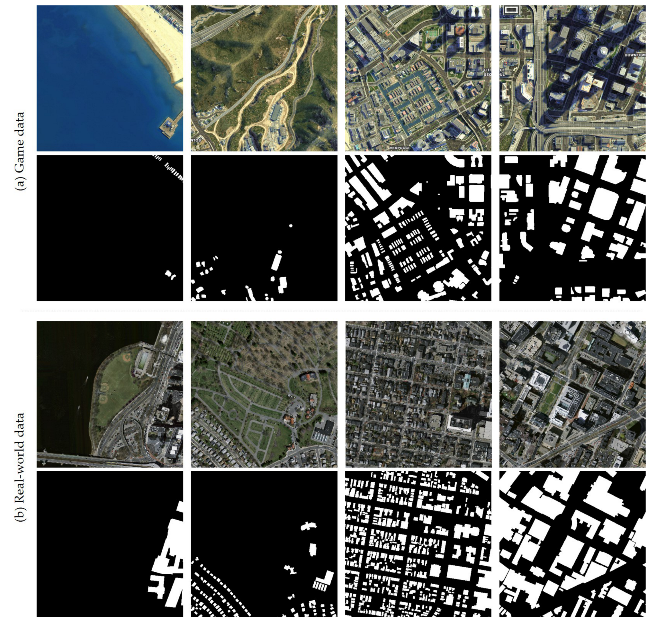
We build our aerial view image segmentation dataset based on the game map of the video game GTA-V. We use a sub-region of the rendered satellite map as our training data. This part of the map is located in the urban part of the fictional city “Los Santos”. We build its ground truth map based on its official legend (8000 × 8000 pixels) by manually annotating the building regions. As the GTA-V official map contains a Google map fashion color legend for various ground features, the manual annotation can be very efficient—it only takes half an hour for a single person to complete the annotation. Our dataset covers the most ground features of a typical coastal city, for example, building, road, green-land, mountain, beach, harbor, wasteland, and so forth. In Figure 3, the first two rows show some representative samples and their ground truth of our synthetic dataset.
We test our model on a real-world remote sensing dataset, the Massachusetts building detection dataset [30]. As the CycleGAN focuses on reducing image style differences between two sets of images, which requires the two datasets to have similar contents. Therefore, a subset of the Massachusetts building dataset is used as our test set. Most of the images in this subset are captured above the urban area. All images in our training and test sets are cropped to image slices with a size of pixels and with the resolution of ∼1 m/pixel before being fed into our networks. Table 1 gives the statistics of our experimental datasets.
The Intersection Over Union (IOU), which is commonly used in previous building segmentation literature [63,64], is used as our evaluation metric for the segmentation results. Given a segmentation output and a ground truth reference image with the same size, the IOU is defined as follows:
where represents the number of true positive pixels, represents the number of false positive pixels and represents the number of false negative pixels in the segmentation output.
3. Results
In our experiment, we first compare our method with some state-of-the-art image segmentation models. Then the ablation analysis is made to evaluate the effectiveness of each of our technical components. Finally, some additional controlled experiments are made to investigate whether the integration of semantic labels helps style conversion.
3.1. Comparison with Other Methods
We compare our model with some state-of-the-art semantic segmentation models, including Deeplab-v3 [29] and UNet [31]. These models are first trained on our game data and then directly tested on the real-world test set without the help of the style transfer. All models are fully optimized for a fair comparison. For each of these methods, we individually train each model for five times and then record the accuracy of each model on our test set (marked as “Test-1”∼“Test-5”).
Table 2 shows their accuracy during the five repeated tests. It should be noticed that although we do not apply any other tricks (e.g., feature fusion and dilated convolution) to increase the feature resolution, as those are used in UNet [31] and Deeplab-v3 [29], our method still achieves the best results in terms of both mean accuracy and stability (standard deviation).
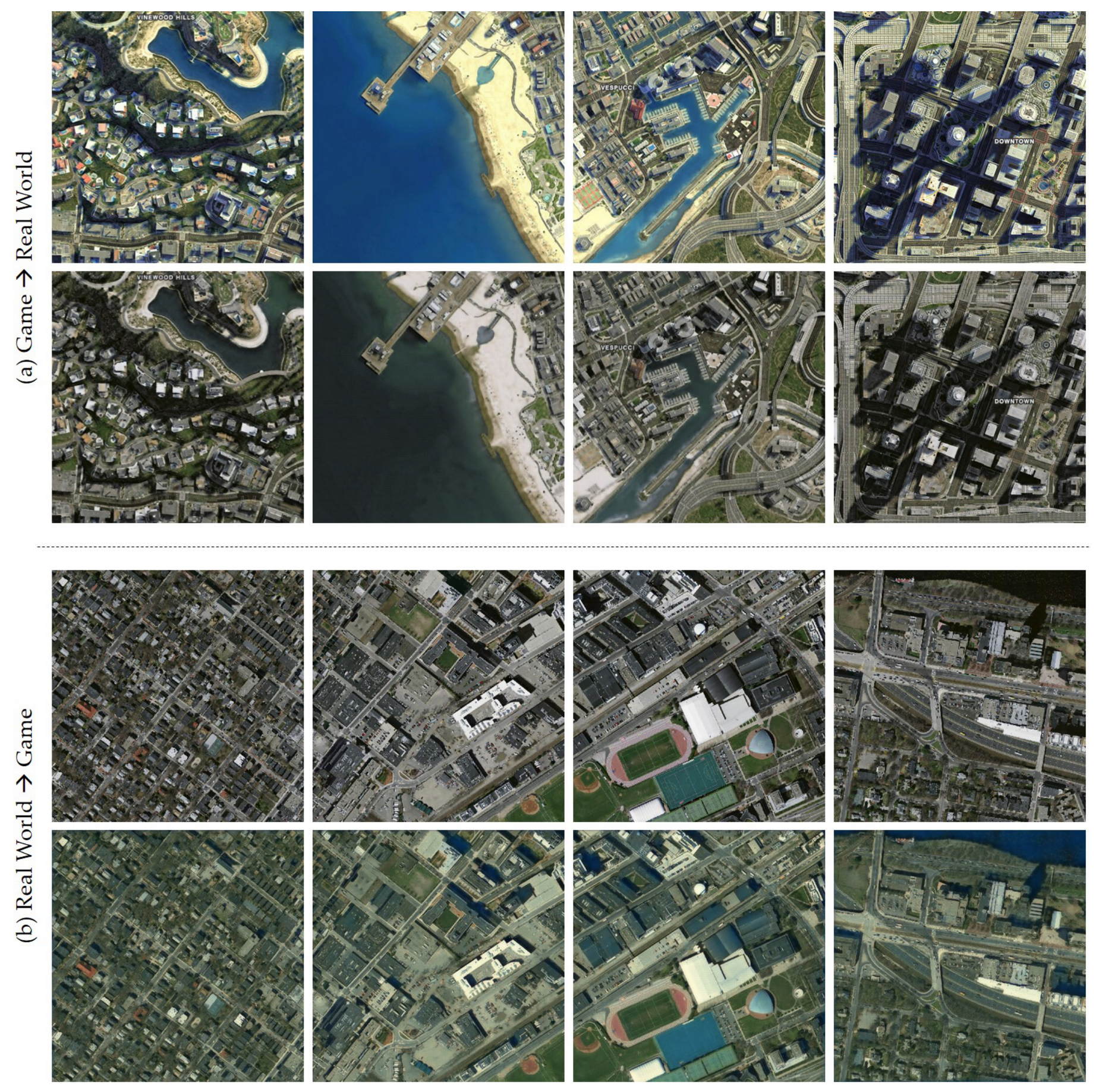
Figure 4 shows some image translation results of our method, where the first two rows show some rendered game images and the “game → real world” translation results. The second two rows show some real world images from the Massachusetts building dataset and the “real world → game” translation results. We can see that the style of these images is transformed to another domain while their contents are retained at the same time.
It is noted that, although some recent modifications on UNet or Deeplab (e.g., TreeUNet [65], MDN [66] and DE-Net [67]) could bring incremental results for remote sensing data, these methods are not designed for the cross-domain segmentation problem. Besides, the source code of the above modifications [65,66,67] is not available at this time and thus cannot be fairly compared. Therefore, we did not compare to these methods.
We have also compared the inference speed of our model with other segmentation methods. It should be noted that although our model consists of five networks (, , , and F), at the inference stage, the computational overhead is only related with the segmentation network F since the CycleGAN part of our model can be simple discarded after training. All our experiments are conducted on a PC platform with a 2080Ti GPU and an I7-7700k CPU. The input image size is set to 500 × 500 pixels. The average inference speed (fps, frames per second) of the UNet, Deeplab-v3 and the proposed method are shown in Table 3. It is shown that our method has comparable inference speed with the Deeplab-v3 but is much faster than the UNet.
3.2. Ablation Analysis
To further evaluate the effectiveness of the proposed methods, the ablation experiment is conducted to verify the importance of each part of our modification, including the “domain adaptation” (Adaptation) and the “end-to-end training” (End-to-End). For a fair comparison, we set our method and its variants with the same experimental configurations in data augmentation and use the same training hyper-parameters. We first compare with a weak baseline method “ResNet50-FCN” where our segmentation network F is only trained according to Equation (6) without the help of adversarial domain adaptation (the first row in Table 4). Then, we gradually add other technical components.
- Res50-FCN: We train our segmentation network F according to Equation (6). The training is performed on game data and then the evaluation is performed on real data without the help of domain adaption (our weak baseline).
- Adaptation: We first train a CycleGAN model separately to transform the game data to the real-world data style. Then we train our segmentation network F based on the transformed data by freezing the parameters of the CycleGAN part (our strong baseline).
- End-to-End: we jointly train the CycleGAN and our segmentation network F according to Equation (8) in an end-to-end fashion (our full implementation).
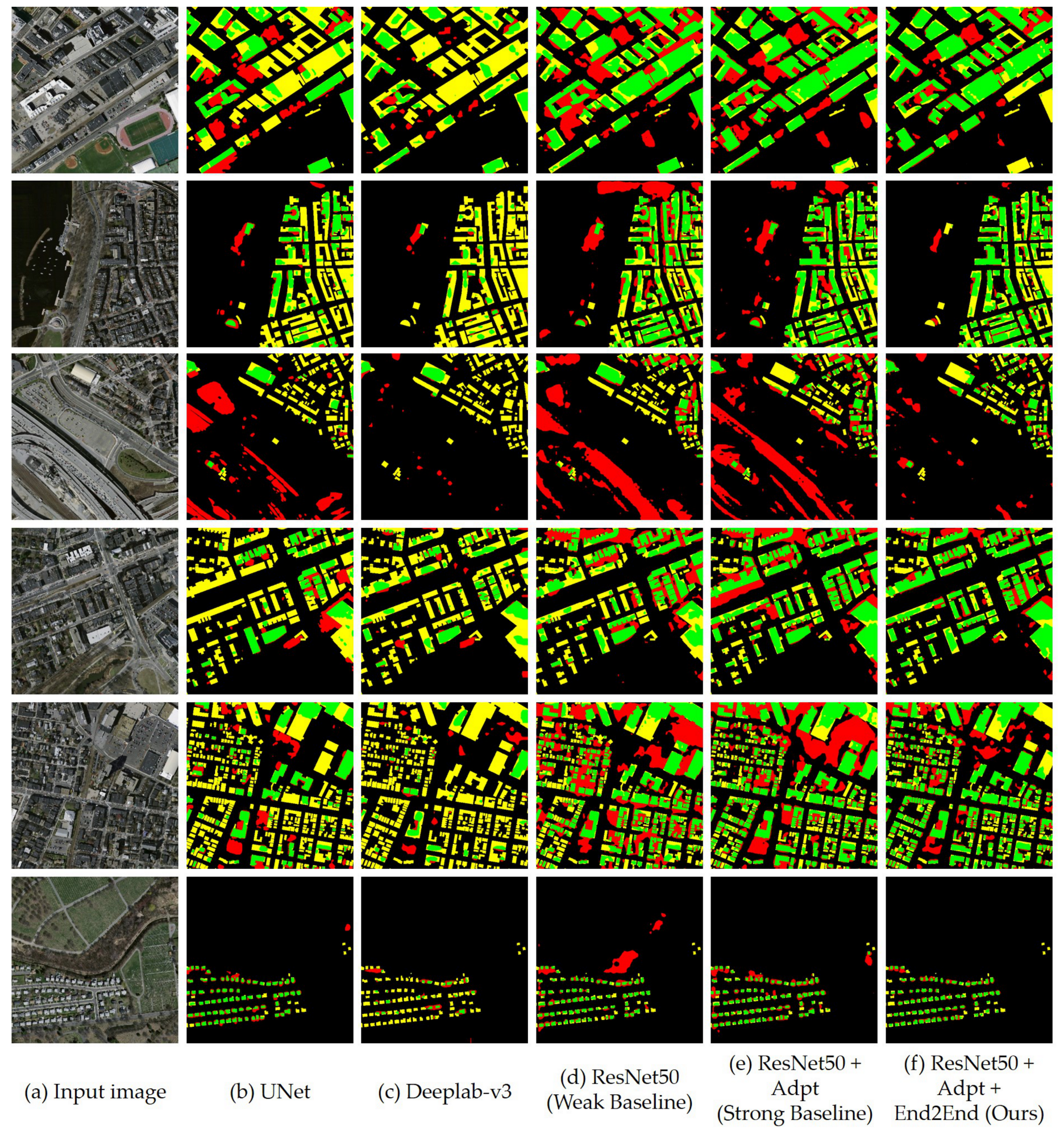
Table 4 shows the evaluation results of all the above variants. We can see the integration of domain adaptation and end-to-end learning yields noticeable improvements in the segmentation accuracy. Figure 5 shows some building segmentation results of the UNet [31], Deeplab-v3 [29] and all the above-mentioned ablation variants. The green, yellow and red pixels represent “true positive” pixels, “false negative” pixels and “false positive” pixels, respectively. Although the style transfer (Res50FCN+Adaptation, our strong baseline) improves the segmentation result, it still has some limitations. As shown in the 3rd row of the Figure 5, the flyover is falsely labeled as building by the UNet, ResNet50 and ResNet50-Adpt, while our end-to-end model (full-implementation) can effectively remove most false-alarms. This improvement (∼4%) is mainly owing to the introduction of semantic information, which benefits our method in generating more precisely stylized results. This indicates that the integration of the semantic information to the style transfer process helps to reduce the style difference between two datasets and thus a semantic segmentation model jointly trained with a style transfer model yields incremental segmentation results. Another reason for the improvement is due to the perturbation of the data introduced by the end-to-end training process, where the intermediate results produced by the CycleGAN produces small input variations to the segmentation network. This variation can be considered as a data augmentation process, which helps improve the generalization ability.
4. Discussion
Do Semantic Labels Help Style Conversion?
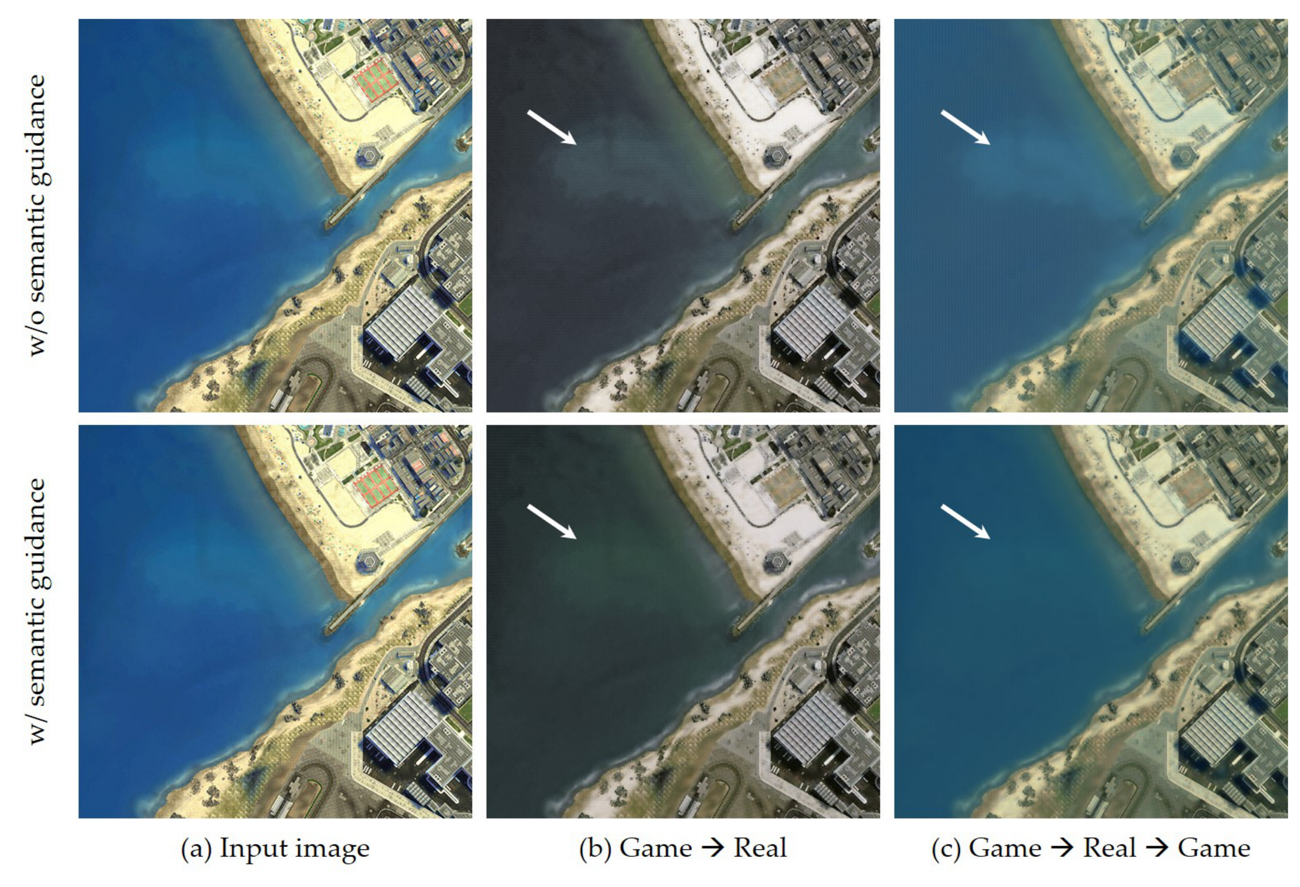
Another advantage of our end-to-end training framework is that it introduces semantic information to the style transfer framework and thus it will benefit to style conversion. Figure 6 gives a comparison example with or without the help of semantic guidance when performing the CycleGAN style conversion. There are subtle differences in the results produced by using the two configurations. The stylized images generated by our end-to-end trained CGFCN are much similar to the images from the target domain than those of the original CycleGAN [26]. This improvement helps in generating more accurate segmentation results.
To further evaluate the style transfer results, we quantitatively compare with CycleGAN on their generated images, as shown in Table 5. We use three image similarity evaluation metrics?(1) the Peak Signal-to-Noise Ratio (PSNR), (2) the Structural Similarity (SSIM) index [68] and (3) the Fréchet Inception Distance (FID) [69]. The PSNR and SSIM two are classic metrics for evaluating image restoration results. The FID is a more recent popular metric that can better evaluate the visual perceptual quality. The FID measures the deviation of the feature distribution between the generated images and the real images, which is widely used in adversarial image synthesis. It should be noticed that although the PSNR and SSIM are computed by comparing the resulting image to a reference image, which requires paired inputs, the FID can be evaluated free from such restrictions. As there is no ground truth reference in the “Game → Real” experiment, we only report the FID score in Table 5. To do this, we randomly divide the generated results and the real data into five groups and then compute the average FID similarity of them. We evaluate the style conversion results of two settings: (1) “game → real-world” conversion and (2) “game → real-world → game” conversion. Our method achieves the best conversion results in all evaluation metrics.
5. Conclusions
We investigate an interesting question that whether game data generalize well for remote sensing image segmentation. To do this, we train a deep learning model on the city map of the game “GTA-V” and then adapt the model to real-world remote sensing building segmentation tasks. To tackle the “domain shift” problem, we propose a CycleGAN-based FCN model where the mappings between the two domains are jointly learned with the building segmentation network. By using the above methods, we have obtained promising results. Experimental results suggest the effectiveness of our method for both segmentation and style conversion.
The applications of our method may not be limited to building segmentation. In fact, our method can be applied to any remote sensing tasks with the problem of “domain shift”—when the source domain and target domain do not share the same data distribution. For example, our method can be applied to road segmentation, vehicle detection, cloud detection, and so forth. Apart from the game data, other types of synthetic data (e.g., architectural rendering data) may also be beneficial to the above remote sensing applications. Besides, since the annotation of game data can be automatically generated, our method can also be used to solve the problem of semi-supervised or unsupervised learning in the remote sensing field.
Author Contributions
Conceptualization, Z.S.; Methodology, Z.Z. (Zhengxia Zou) and T.S.; Validation, T.S. and W.L.; Formal Analysis, Z.S., Z.Z. (Zhengxia Zou), and Z.Z. (Zhou Zhang); Writing and original draft preparation: Z.Z. (Zhengxia Zou) and T.S.; Writing—Review and Editing, Z.S., T.S., Z.Z. (Zhou Zhang) and Z.Z. (Zhengxia Zou). All authors have read and agreed to the published version of the manuscript.
Funding
The work was supported by the National Key R&D Program of China under the Grant 2017YFC1405605, the National Natural Science Foundation of China under the Grant 61671037, the Beijing Natural Science Foundation under the Grant 4192034 and the National Defense Science and Technology Innovation Special Zone Project.
Conflicts of Interest
The authors declare no conflict of interest.
References
- LeCun, Y.; Bengio, Y.; Hinton, G. Deep learning. Nature 2015, 521, 436. [Google Scholar] [CrossRef] [PubMed]
- Goodfellow, I.; Bengio, Y.; Courville, A. Deep Learning; MIT Press: Cambridge, MA, USA, 2016. [Google Scholar]
- Zhang, L.; Zhang, L.; Du, B. Deep learning for remote sensing data: A technical tutorial on the state of the art. IEEE Geosci. Remote Sens. Mag. 2016, 4, 22–40. [Google Scholar] [CrossRef]
- Zou, Z.; Shi, Z. Random access memories: A new paradigm for target detection in high resolution aerial remote sensing images. IEEE Trans. Image Process. 2018, 27, 1100–1111. [Google Scholar] [CrossRef]
- Shi, Z.; Zou, Z. Can a machine generate humanlike language descriptions for a remote sensing image? IEEE Trans. Geosci. Remote Sens. 2017, 55, 3623–3634. [Google Scholar] [CrossRef]
- Penatti, O.A.; Nogueira, K.; Dos Santos, J.A. Do deep features generalize from everyday objects to remote sensing and aerial scenes domains? In Proceedings of the IEEE Conference on Computer Vision and Pattern Recognition Workshops, Boston, MA, USA, 7–12 June 2015; pp. 44–51. [Google Scholar]
- Xia, G.S.; Bai, X.; Ding, J.; Zhu, Z.; Belongie, S.; Luo, J.; Datcu, M.; Pelillo, M.; Zhang, L. DOTA: A large-scale dataset for object detection in aerial images. In Proceedings of the IEEE Conference on Computer Vision and Pattern Recognition, Salt Lake City, UT, USA, 18–23 June 2018; pp. 3974–3983. [Google Scholar]
- Patel, V.M.; Gopalan, R.; Li, R.; Chellappa, R. Visual domain adaptation: A survey of recent advances. IEEE Signal Process. Mag. 2015, 32, 53–69. [Google Scholar] [CrossRef]
- Fernando, B.; Habrard, A.; Sebban, M.; Tuytelaars, T. Unsupervised visual domain adaptation using subspace alignment. In Proceedings of the IEEE International Conference on Computer Vision, Sydney, NSW, Australia, 1–8 December 2013; pp. 2960–2967. [Google Scholar]
- Wang, M.; Deng, W. Deep visual domain adaptation: A survey. Neurocomputing 2018, 312, 135–153. [Google Scholar] [CrossRef] [Green Version]
- Yao, T.; Pan, Y.; Ngo, C.W.; Li, H.; Mei, T. Semi-supervised domain adaptation with subspace learning for visual recognition. In Proceedings of the IEEE Conference on Computer Vision and Pattern Recognition, Boston, MA, USA, 7–12 June 2015; pp. 2142–2150. [Google Scholar]
- Ros, G.; Sellart, L.; Materzynska, J.; Vazquez, D.; Lopez, A.M. The synthia dataset: A large collection of synthetic images for semantic segmentation of urban scenes. In Proceedings of the IEEE Conference on Computer Vision and Pattern Recognition, Las Vegas, NV, USA, 27–30 June 2016; pp. 3234–3243. [Google Scholar]
- Richter, S.R.; Vineet, V.; Roth, S.; Koltun, V. Playing for data: Ground truth from computer games. In Proceedings of the European Conference on Computer Vision, Amsterdam, The Netherlands, 11–14 October 2016; pp. 102–118. [Google Scholar]
- Zhang, Y.; Qiu, Z.; Yao, T.; Liu, D.; Mei, T. Fully Convolutional Adaptation Networks for Semantic Segmentation. In Proceedings of the IEEE Conference on Computer Vision and Pattern Recognition, Salt Lake City, UT, USA, 18–23 June 2018; pp. 6810–6818. [Google Scholar]
- Hoffman, J.; Tzeng, E.; Park, T.; Zhu, J.Y.; Isola, P.; Saenko, K.; Efros, A.A.; Darrell, T. Cycada: Cycle-consistent adversarial domain adaptation. arXiv 2017, arXiv:1711.03213. [Google Scholar]
- Tzeng, E.; Hoffman, J.; Saenko, K.; Darrell, T. Adversarial discriminative domain adaptation. In Proceedings of the IEEE Conference on Computer Vision and Pattern Recognition, Honolulu, HI, USA, 21–26 July 2017; pp. 7167–7176. [Google Scholar]
- Sankaranarayanan, S.; Balaji, Y.; Jain, A.; Nam Lim, S.; Chellappa, R. Learning from synthetic data: Addressing domain shift for semantic segmentation. In Proceedings of the IEEE Conference on Computer Vision and Pattern Recognition, Salt Lake City, UT, USA, 18–23 June 2018; pp. 3752–3761. [Google Scholar]
- Gatys, L.A.; Ecker, A.S.; Bethge, M. Image Style Transfer Using Convolutional Neural Networks. In Proceedings of the 2016 IEEE Conference on Computer Vision and Pattern Recognition (CVPR), Las Vegas, NV, USA, 27–30 June 2016; pp. 2414–2423. [Google Scholar]
- Lu, M.; Zhao, H.; Yao, A.; Xu, F.; Chen, Y.; Zhang, L. Decoder network over lightweight reconstructed feature for fast semantic style transfer. In Proceedings of the IEEE Conference on Computer Vision and Pattern Recognition, Honolulu, HI, USA, 21–26 July 2017; pp. 2469–2477. [Google Scholar]
- Li, Y.; Fang, C.; Yang, J.; Wang, Z.; Lu, X.; Yang, M.H. Universal style transfer via feature transforms. In Proceedings of the Annual Conference on Neural Information Processing Systems, Long Beach, CA, USA, 4–9 December 2017; pp. 386–396. [Google Scholar]
- Liao, J.; Yao, Y.; Yuan, L.; Hua, G.; Kang, S.B. Visual attribute transfer through deep image analogy. ACM Trans. Graphics 2017, 36, 120. [Google Scholar] [CrossRef] [Green Version]
- Goodfellow, I.; Pouget-Abadie, J.; Mirza, M.; Xu, B.; Warde-Farley, D.; Ozair, S.; Courville, A.; Bengio, Y. Generative adversarial nets. In Proceedings of the Annual Conference on Neural Information Processing Systems, Montreal, QC, Canada, 8–13 December 2014; pp. 2672–2680. [Google Scholar]
- Goodfellow, I. NIPS 2016 tutorial: Generative adversarial networks. arXiv 2016, arXiv:1701.00160. [Google Scholar]
- Lu, Y.; Tai, Y.W.; Tang, C.K. Attribute-Guided Face Generation Using Conditional CycleGAN. In Proceedings of the European Conference on Computer Vision (ECCV), Munich, Germany, 8–14 September 2018. [Google Scholar]
- Chang, H.; Lu, J.; Yu, F.; Finkelstein, A. PairedCycleGAN: Asymmetric Style Transfer for Applying and Removing Makeup. In Proceedings of the IEEE Conference on Computer Vision and Pattern Recognition (CVPR), Salt Lake City, UT, USA, 18–22 June 2018. [Google Scholar]
- Zhu, J.Y.; Park, T.; Isola, P.; Efros, A.A. Unpaired Image-To-Image Translation Using Cycle-Consistent Adversarial Networks. In Proceedings of the IEEE International Conference on Computer Vision (ICCV), Venice, Italy, 22–29 October 2017. [Google Scholar]
- Inoue, N.; Furuta, R.; Yamasaki, T.; Aizawa, K. Cross-domain weakly-supervised object detection through progressive domain adaptation. In Proceedings of the IEEE Conference on Computer Vision and Pattern Recognition, Salt Lake City, UT, USA, 18–23 June 2018; pp. 5001–5009. [Google Scholar]
- Long, J.; Shelhamer, E.; Darrell, T. Fully convolutional networks for semantic segmentation. In Proceedings of the IEEE Conference on Computer Vision and Pattern Recognition, Boston, MA, USA, 7–12 June 2015; pp. 3431–3440. [Google Scholar]
- Chen, L.C.; Papandreou, G.; Kokkinos, I.; Murphy, K.; Yuille, A.L. Deeplab: Semantic image segmentation with deep convolutional nets, atrous convolution, and fully connected crfs. IEEE Trans. Pattern Anal. Mach. Intell. 2018, 40, 834–848. [Google Scholar] [CrossRef]
- Mnih, V. Machine Learning for Aerial Image Labeling; University of Toronto: Toronto, ON, Canada, 2013. [Google Scholar]
- Ronneberger, O.; Fischer, P.; Brox, T. U-net: Convolutional networks for biomedical image segmentation. In Proceedings of the International Conference on Medical Image Computing And Computer-Assisted Intervention, Munich, Germany, 5–9 October 2015; pp. 234–241. [Google Scholar]
- Krizhevsky, A.; Sutskever, I.; Hinton, G.E. Imagenet classification with deep convolutional neural networks. In Proceedings of the Annual Conference on Neural Information Processing Systems, Lake Tahoe, NV, USA, 3–6 December 2012; pp. 1097–1105. [Google Scholar]
- Simonyan, K.; Zisserman, A. Very deep convolutional networks for large-scale image recognition. arXiv 2014, arXiv:1409.1556. [Google Scholar]
- Szegedy, C.; Vanhoucke, V.; Ioffe, S.; Shlens, J.; Wojna, Z. Rethinking the inception architecture for computer vision. In Proceedings of the IEEE Conference on Computer Vision and Pattern Recognition, Las Vegas, NV, USA, 27–30 June 2016; pp. 2818–2826. [Google Scholar]
- He, K.; Zhang, X.; Ren, S.; Sun, J. Deep residual learning for image recognition. In Proceedings of the IEEE Conference on Computer Vision and Pattern Recognition, Las Vegas, NV, USA, 27–30 June 2016; pp. 770–778. [Google Scholar]
- Zou, Z.; Shi, Z.; Guo, Y.; Ye, J. Object Detection in 20 Years: A Survey. arXiv 2019, arXiv:1905.05055. [Google Scholar]
- Girshick, R.; Donahue, J.; Darrell, T.; Malik, J. Rich feature hierarchies for accurate object detection and semantic segmentation. In Proceedings of the IEEE Conference on Computer Vision and Pattern Recognition, Columbus, OH, USA, 23–28 June 2014; pp. 580–587. [Google Scholar]
- Girshick, R. Fast r-cnn. In Proceedings of the IEEE International Conference on Computer Vision, Santiago, Chile, 7–13 December 2015; pp. 1440–1448. [Google Scholar]
- Ren, S.; He, K.; Girshick, R.; Sun, J. Faster r-cnn: Towards real-time object detection with region proposal networks. In Proceedings of the Advances in Neural Information Processing Systems, Montreal, QC, Canada, 7–12 December 2015; pp. 91–99. [Google Scholar]
- Redmon, J.; Divvala, S.; Girshick, R.; Farhadi, A. You only look once: Unified, real-time object detection. In Proceedings of the IEEE Conference on Computer Vision and Pattern Recognition, Las Vegas, NV, USA, 27–30 June 2016; pp. 779–788. [Google Scholar]
- Liu, W.; Anguelov, D.; Erhan, D.; Szegedy, C.; Reed, S.; Fu, C.Y.; Berg, A.C. Ssd: Single shot multibox detector. In Proceedings of the European Conference on Computer Vision, Amsterdam, The Netherlands, 11–14 October 2016; pp. 21–37. [Google Scholar]
- Noh, H.; Hong, S.; Han, B. Learning deconvolution network for semantic segmentation. In Proceedings of the IEEE International Conference on Computer Vision, Santiago, Chile, 7–13 December 2015; pp. 1520–1528. [Google Scholar]
- Chen, L.C.; Papandreou, G.; Kokkinos, I.; Murphy, K.; Yuille, A.L. Semantic Image Segmentation with Deep Convolutional Nets and Fully Connected CRFs. In Proceedings of the ICLR, San Diego, CA, USA, 7–9 May 2015. [Google Scholar]
- Karpathy, A.; Fei-Fei, L. Deep visual-semantic alignments for generating image descriptions. In Proceedings of the IEEE Conference on Computer Vision and Pattern Recognition, Boston, MA, USA, 7–12 June 2015; pp. 3128–3137. [Google Scholar]
- Xu, K.; Ba, J.; Kiros, R.; Cho, K.; Courville, A.; Salakhudinov, R.; Zemel, R.; Bengio, Y. Show, attend and tell: Neural image caption generation with visual attention. In Proceedings of the International Conference on Machine Learning, Lille, France, 6–11 July 2015; pp. 2048–2057. [Google Scholar]
- Wu, Q.; Shen, C.; Wang, P.; Dick, A.; van den Hengel, A. Image captioning and visual question answering based on attributes and external knowledge. IEEE Trans. Pattern Anal. Mach. Intell. 2017, 40, 1367–1381. [Google Scholar] [CrossRef] [PubMed] [Green Version]
- Dong, C.; Loy, C.C.; He, K.; Tang, X. Image super-resolution using deep convolutional networks. IEEE Trans. Pattern Anal. Mach. Intell. 2015, 38, 295–307. [Google Scholar] [CrossRef] [PubMed] [Green Version]
- Kim, J.; Kwon Lee, J.; Mu Lee, K. Accurate image super-resolution using very deep convolutional networks. In Proceedings of the IEEE Conference on Computer Vision and Pattern Recognition, Las Vegas, NV, USA, 27–30 June 2016; pp. 1646–1654. [Google Scholar]
- Ledig, C.; Theis, L.; Huszár, F.; Caballero, J.; Cunningham, A.; Acosta, A.; Aitken, A.; Tejani, A.; Totz, J.; Wang, Z.; et al. Photo-realistic single image super-resolution using a generative adversarial network. In Proceedings of the IEEE Conference on Computer Vision and Pattern Recognition, Honolulu, HI, USA, 21–26 July 2017; pp. 4681–4690. [Google Scholar]
- Denton, E.L.; Chintala, S.; Fergus, R.; Szlam, A. Deep generative image models using a laplacian pyramid of adversarial networks. In Proceedings of the Advances in Neural Information Processing Systems, Montreal, QC, Canada, 7–12 December 2015; pp. 1486–1494.
- Radford, A.; Metz, L.; Chintala, S. Unsupervised representation learning with deep convolutional generative adversarial networks. arXiv 2015, arXiv:1511.06434. [Google Scholar]
- Zhang, H.; Goodfellow, I.; Metaxas, D.; Odena, A. Self-attention generative adversarial networks. arXiv 2018, arXiv:1805.08318. [Google Scholar]
- Brock, A.; Donahue, J.; Simonyan, K. Large scale gan training for high fidelity natural image synthesis. arXiv 2018, arXiv:1809.11096. [Google Scholar]
- Isola, P.; Zhu, J.Y.; Zhou, T.; Efros, A.A. Image-to-image translation with conditional adversarial networks. In Proceedings of the IEEE Conference on Computer Vision and Pattern Recognition, Honolulu, HI, USA, 21–26 July 2017; pp. 1125–1134. [Google Scholar]
- Choi, Y.; Choi, M.; Kim, M.; Ha, J.W.; Kim, S.; Choo, J. Stargan: Unified generative adversarial networks for multi-domain image-to-image translation. In Proceedings of the IEEE Conference on Computer Vision and Pattern Recognition, Salt Lake City, UT, USA, 18–23 June 2018; pp. 8789–8797. [Google Scholar]
- Li, J.; Liang, X.; Wei, Y.; Xu, T.; Feng, J.; Yan, S. Perceptual generative adversarial networks for small object detection. In Proceedings of the IEEE CVPR, Honolulu, HI, USA, 21–26 July 2017. [Google Scholar]
- Bai, Y.; Zhang, Y.; Ding, M.; Ghanem, B. SOD-MTGAN: Small Object Detection via Multi-Task Generative Adversarial Network. In Proceedings of the Computer Vision-ECCV, Munich, Germany, 8–14 September 2018; pp. 8–14. [Google Scholar]
- Wang, X.; Shrivastava, A.; Gupta, A. A-fast-rcnn: Hard positive generation via adversary for object detection. In Proceedings of the IEEE Conference on Computer Vision and Pattern Recognition, Honolulu, HI, USA, 21–26 July 2017. [Google Scholar]
- Wang, X.; Yu, K.; Wu, S.; Gu, J.; Liu, Y.; Dong, C.; Qiao, Y.; Change Loy, C. Esrgan: Enhanced super-resolution generative adversarial networks. In Proceedings of the European Conference on Computer Vision (ECCV), Munich, Germany, 8–14 September 2018. [Google Scholar]
- Yuan, Y.; Liu, S.; Zhang, J.; Zhang, Y.; Dong, C.; Lin, L. Unsupervised image super-resolution using cycle-in-cycle generative adversarial networks. In Proceedings of the IEEE Conference on Computer Vision and Pattern Recognition Workshops, Salt Lake City, UT, USA, 18–22 June 2018; pp. 701–710. [Google Scholar]
- Kingma, D.P.; Ba, J. Adam: A method for stochastic optimization. arXiv 2014, arXiv:1412.6980. [Google Scholar]
- Deng, J.; Dong, W.; Socher, R.; Li, L.J.; Li, K.; Fei-Fei, L. Imagenet: A large-scale hierarchical image database. In Proceedings of the IEEE Conference on Computer Vision and Pattern Recognition (CVPR), Miami, FL, USA, 20–25 June 2009; pp. 248–255. [Google Scholar]
- Ji, S.; Wei, S.; Lu, M. Fully Convolutional Networks for Multisource Building Extraction from an Open Aerial and Satellite Imagery Data Set. IEEE Trans. Geosci. Remote Sens. 2019, 57, 574–586. [Google Scholar] [CrossRef]
- Maggiori, E.; Tarabalka, Y.; Charpiat, G.; Alliez, P. Convolutional Neural Networks for Large-Scale Remote-Sensing Image Classification. IEEE Trans. Geosci. Remote Sens. 2017, 55, 645–657. [Google Scholar] [CrossRef] [Green Version]
- Yue, K.; Yang, L.; Li, R.; Hu, W.; Zhang, F.; Li, W. TreeUNet: Adaptive Tree convolutional neural networks for subdecimeter aerial image segmentation. ISPRS J. Photogramm. Remote Sens. 2019, 156, 1–13. [Google Scholar] [CrossRef]
- Zhang, X.; Xiao, Z.; Li, D.; Fan, M.; Zhao, L. Semantic Segmentation of Remote Sensing Images Using Multiscale Decoding Network. IEEE Geosci. Remote Sens. Lett. 2019, 16, 1492–1496. [Google Scholar] [CrossRef]
- Liu, H.; Luo, J.; Huang, B.; Hu, X.; Sun, Y.; Yang, Y.; Xu, N.; Zhou, N. DE-Net: Deep Encoding Network for Building Extraction from High-Resolution Remote Sensing Imagery. Remote Sens. 2019, 11, 2380. [Google Scholar] [CrossRef] [Green Version]
- Wang, Z.; Bovik, A.C.; Sheikh, H.R.; Simoncelli, E.P. Image quality assessment: From error visibility to structural similarity. IEEE Trans. Image Process. 2004, 13, 600–612. [Google Scholar] [CrossRef] [PubMed] [Green Version]
- Heusel, M.; Ramsauer, H.; Unterthiner, T.; Nessler, B.; Hochreiter, S. Gans trained by a two time-scale update rule converge to a local nash equilibrium. In Proceedings of the Advances in Neural Information Processing Systems, Long Beach, CA, USA, 4–9 December 2017; pp. 6626–6637. [Google Scholar]
Figure 1.
An official map of the video game Grand Theft Auto-V (GTA-V): the city of Los Santos. (a) The satellite imagery rendered from aerial view. (b) An in-game frame rendered from the “first-person perspective”. (c) A part of the game map that is used in our experiment. (d) The legend of the map (in a similar fashion of Google maps). Different to the previous datasets [12,13] that focuses on rendering street-view images from the “first-person perspective” (like (b)), we build our dataset from the “aerial perspective” of the city (c,d).

Figure 2.
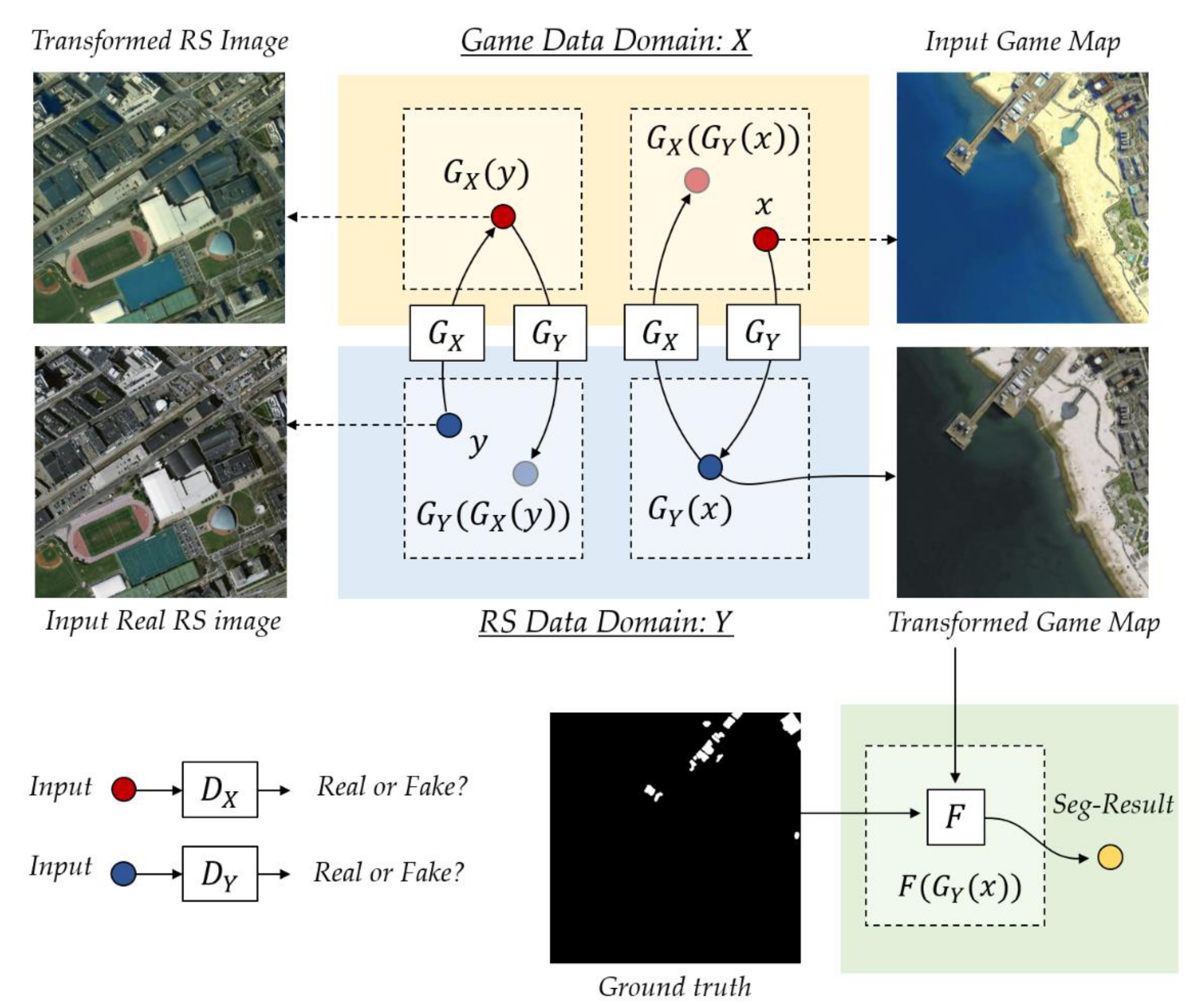
An overview of the proposed method. Our method consists of five networks: , , , and F. The former four networks, which corresponds to a CycleGAN model [26], learn two mappings between the game domain X and the remote sensing domain Y (, ). The last network F learns to predict building masks of the transformed data. In our method, we first transfer the style of a synthetic game map x to a real one and then train the network F based on the transformed image (input) and the game map legend (ground truth).
Figure 2.
An overview of the proposed method. Our method consists of five networks: , , , and F. The former four networks, which corresponds to a CycleGAN model [26], learn two mappings between the game domain X and the remote sensing domain Y (, ). The last network F learns to predict building masks of the transformed data. In our method, we first transfer the style of a synthetic game map x to a real one and then train the network F based on the transformed image (input) and the game map legend (ground truth).

Figure 3.
A preview of our two experimental datasets. (a) The first two rows show some representative images and their ground truth labels from our synthetic dataset (our training and validation set). (b) The last two rows show some image pairs from the real remote sensing dataset [30] (our testing set).

Figure 4.
(Better viewed in color) Some image translation results from using our method. (a) The first two rows show the translation results from the game domain to the real-world domain. (b) The last two rows show the inverse translation results from the real-world domain to the game domain.
Figure 4.
(Better viewed in color) Some image translation results from using our method. (a) The first two rows show the translation results from the game domain to the real-world domain. (b) The last two rows show the inverse translation results from the real-world domain to the game domain.

Figure 5.
(Better viewed in color) Some building segmentation results of different methods: (a) Input Image, (b) UNet [31], (c) Deeplab-v3 [29], (d) ResNet50-FCN (our weak baseline), (e) ResNet50-FCN + Adapt (our strong baseline) and (f) ResNet50-FCN + Adapt + End2End (our full implementation). Green pixels: true positives. Yellow pixels: false negatives. Red pixels: false positives.

Figure 6.
(Better viewed in color) A visual comparison of style transfer results with different configurations. The first row corresponds to the results of the original CycleGAN [26] and the second row corresponds to the results of our method. Columns: (a) input game data, (b) game → real, (c) game → real → game. We can see that the images generated by our method are closer to the target domain and thus helps cross-domain segmentation. Some unrelated image contents (e.g., the pollution area marked by the arrows) have been successfully removed during the conversion.


Table 1.
Statistics of our experimental datasets. We first train our model on the synthetic remote sensing dataset (GTA-V game map) and then run evaluation on the real remote sensing dataset (Massachusetts Building).
Table 1.
Statistics of our experimental datasets. We first train our model on the synthetic remote sensing dataset (GTA-V game map) and then run evaluation on the real remote sensing dataset (Massachusetts Building).
| Dataset | Synthetic Remote Sensing Dataset | Real Remote Sensing Dataset |
|---|---|---|
| Image Source | GTA-V Game Map (Los Santos) | Massachusetts Building [30] |
| Number of Images | 121 | 150 (a subset) |
| Image Size | 500 × 500 pixel | 500 × 500 pixel |
| Resolution | ∼1.0 m/pixel | 1.0 m/pixel |
| Eval Split | Trainig/Evaluation Set | Testing Set |
Table 2.
A comparison of different methods: UNet [31], Deeplab-v3 [29] and CycleGAN based Fully Convolutional Networks (CGFCN) (Ours). All methods are trained based on the synthetic data and then tested on real data. For each of these methods, we individually train each model for five times and then record the accuracy of each model on our test set (marked as “Test-1”∼“Test-5”). The CGFCN obtains the best results in both mean accuracy and stability.
| Metric | UNet [31] | Deeplab-v3 [29] | CGFCN (Ours) |
|---|---|---|---|
| IOU (Test 1) | 0.1592 | 0.1822 | 0.5218 |
| IOU (Test 2) | 0.2623 | 0.1715 | 0.5253 |
| IOU (Test 3) | 0.2837 | 0.1562 | 0.5220 |
| IOU (Test 4) | 0.2175 | 0.2022 | 0.5042 |
| IOU (Test 5) | 0.2586 | 0.2025 | 0.5355 |
| Average | 0.2363 | 0.1829 | 0.5218 |
| Stdev (±) | 0.0441 | 0.0179 | 0.0101 |
Table 3.
Average inference speed (frames per second) of different models.
| Methods | Inference Speed (fps) |
|---|---|
| UNet [31] | 14.262 |
| Deeplab-v3 [29] | 21.838 |
| CGFCN (Ours) | 21.857 |
Table 4.
Results of our ablation analysis on “domain adaptation” and “end-to-end training”. Res50FCN: our baseline method. Adaptation: the style transfer networks (, ) and segmentation network F are separately trained. En2En: jointly train all networks in an end-to-end fashion. The integration of the domain adaptation and end-to-end learning yields noticeable improvements in the segmentation accuracy.
| Ablations | Segmentation Accuracy (IOU) on Game Dataset | |||||||
|---|---|---|---|---|---|---|---|---|
| Res50FCN | Adaptation | En2En | Test 1 | Test 2 | Test 3 | Test 4 | Test 5 | Average ± Stdev |
| ✓ | 0.4322 | 0.4146 | 0.4299 | 0.4342 | 0.4427 | 0.4307 ± 0.0091 | ||
| ✓ | ✓ | 0.4708 | 0.4905 | 0.4753 | 0.4991 | 0.4785 | 0.4828 ± 0.0104 | |
| ✓ | ✓ | ✓ | 0.5218 | 0.5253 | 0.5220 | 0.5042 | 0.5355 | 0.5218 ± 0.0101 |
Table 5.
Evaluation results on image style transfer results with different similarity evaluation metrics: Fréchet Inception Distance (FID) [69], Peak Signal-to-Noise Ratio (PSNR) and Structural Similarity (SSIM) [68]. The column “Game → Real”: we compute the similarity between a group of the real images and generated ones. The column “Game → Real → Game”: we back-convert the generated image to the game domain and then compute their “self-similarity”. For FID, lower scores indicate better. For PSNR (dB) and SSIM, higher scores indicate better. The CGFCN (ours) achieves the best results, which suggests that introducing semantical supervision helps improve image style conversion.
| Metric | Game → Real | Game → Real → Game | ||
|---|---|---|---|---|
| FID | FID | PSNR | SSIM | |
| CycleGAN | 0.1893 | 0.1078 | 20.575 | 0.7214 |
| CGFCN | 0.1621 | 0.0724 | 20.598 | 0.8038 |
| Game Data | 0.1808 | 0.0000 | +∞ | 1.0000 |
| Reference | Real Data | Game Data | ||
© 2020 by the authors. Licensee MDPI, Basel, Switzerland. This article is an open access article distributed under the terms and conditions of the Creative Commons Attribution (CC BY) license (http://creativecommons.org/licenses/by/4.0/).
Share and Cite
MDPI and ACS Style
Zou, Z.; Shi, T.; Li, W.; Zhang, Z.; Shi, Z. Do Game Data Generalize Well for Remote Sensing Image Segmentation? Remote Sens. 2020, 12, 275. https://0-doi-org.brum.beds.ac.uk/10.3390/rs12020275
AMA Style
Zou Z, Shi T, Li W, Zhang Z, Shi Z. Do Game Data Generalize Well for Remote Sensing Image Segmentation? Remote Sensing. 2020; 12(2):275. https://0-doi-org.brum.beds.ac.uk/10.3390/rs12020275
Chicago/Turabian StyleZou, Zhengxia, Tianyang Shi, Wenyuan Li, Zhou Zhang, and Zhenwei Shi. 2020. "Do Game Data Generalize Well for Remote Sensing Image Segmentation?" Remote Sensing 12, no. 2: 275. https://0-doi-org.brum.beds.ac.uk/10.3390/rs12020275
Note that from the first issue of 2016, this journal uses article numbers instead of page numbers. See further details here.