Sentinel-2 Sharpening via Parallel Residual Network

Abstract

Sentinel-2 data is of great utility for a wide range of remote sensing applications due to its free access and fine spatial-temporal coverage. However, restricted by the hardware, only four bands of Sentinel-2 images are provided at 10 m resolution, while others are recorded at reduced resolution (i.e., 20 m or 60 m). In this paper, we propose a parallel residual network for Sentinel-2 sharpening termed SPRNet, to obtain the complete data at 10 m resolution. The proposed network aims to learn the mapping between the low-resolution (LR) bands and ideal high-resolution (HR) bands by three steps, including parallel spatial residual learning, spatial feature fusing and spectral feature mapping. First, rather than using the single branch network, the parallel residual learning structure is proposed to extract the spatial features from different resolution bands separately. Second, the spatial feature fusing is aimed to fully fuse the extracted features from each branch and produce the residual image with spatial information. Third, to keep spectral fidelity, the spectral feature mapping is utilized to directly propagate the spectral characteristics of LR bands to target HR bands. Without using extra training data, the proposed network is trained with the lower scale data synthesized from the observed Sentinel-2 data and applied to the original ones. The data at 10 m spatial resolution can be finally obtained by feeding the original 10 m, 20 m and 60 m bands to the trained SPRNet. Extensive experiments conducted on two datasets indicate that the proposed SPRNet obtains good results in the spatial fidelity and the spectral preservation. Compared with the competing approaches, the SPRNet increases the SRE by at least 1.538 dB on 20 m bands and 3.188 dB on 60 m bands while reduces the SAM by at least 0.282 on 20 m bands and 0.162 on 60 m bands.

1. Introduction

Sentinel-2 is a wide swath and optical fine resolution satellite imaging mission released by the European Space Agency (ESA) [1]. Owing to frequent revisit rate, global access and free availability, Sentinel-2 products have been widely used to monitor dynamically changing geophysical variables such as vegetation, soil, water cover and coasts [2,3,4,5]. However, due to the storage and transmission bandwidth restrictions, thirteen spectral bands in Sentinel-2 image are acquired with three different spatial resolutions including: four 10 m bands, six 20 m bands and three 60 m bands. With the same spatial coverage, the low-resolution (LR) bands have the potential to be enhanced by image sharpening, which is an economically effective technique that can merge the LR bands with the high-resolution (HR) bands to produce a complete HR image (ideally without loss of spectral information) [6]. With desirable spatial and spectral resolution, the sharpening image can yield better interpretation capabilities in the remote sensing applications [7,8,9].

Plenty of image sharpening methods have been proposed to enhance the spatial resolution of various sensors, such as Moderate Resolution Imaging Spectroradiometer (MODIS) [10], Advanced Spaceborne Theemal Emission and Reflection Radiometer (ASTER) [11], WorldView-2 [12] and more recently for Visible Infrared Imaging Radiometer Suite (VIIRS) [13] and Sentinel-2. These methods can be generally classified into three categories: classic pansharpening-based, model-based, and learning-based methods. Pansharpening is a crucial image enhancement technique which focuses on injecting spatial information extracted from the HR panchromatic (PAN) to LR image. The methods fall into this type including intensity-hue-saturation transform (IHS) [14], Gram-Schmidt (GS) transform, adaptive GS [15] and $\stackrel{‵}{a}$ trous wavelet transform (ATWT) [16], etc. Sentinel-2 sharpening can be taken as an extension of pansharpening, and various pansharpening methods are directly applied to enhance 20 m bands by selecting or synthesising a band from 10 bands as PAN [17,18,19,20]. And the Sentinel-2 pansharpening results have been used for water bodies’ mapping [21] and land-cover classification [22]. However, there are two differences between pansharpening and Sentinel-2 sharpening: (i) four HR bands, rather than a PAN, can be used to sharpen the bands at reduced resolution (i.e., 20 m and 60 m); (ii) the spectral range of HR bands can not overlap the LR ones. Therefore, the applicability of pansharpening-based methods is limited in Sentinel-2 sharpening.

The model-based methods concentrate on constructing the observation models that can describe the explicit process of the image, such as blurring, down-sampling and noise [23]. As an ill-posed problem, these methods simulate the process with prior constraints and the modeling can be conceptually seen as an optimization problem. The representative methods used for sharpening include Bayesian model [24,25] and sparse representation [26]. To address the problem of Sentinel-2 sharpening, several methods are presented by taking this task as a convex optimization problem. For instance, a method called SupReME is proposed [27] to solve a convex deconvolution problem in a low dimensional subspace, which is regularized using the roughness penalty. To extend the SupReME, a cyclic descent based optimization is put forward to find the low dimensional subspace in [28] and a patch-based regularisation is adopted to model the self-similarity of the images in [29]. Reference [30] exploits the object geometric information across the multi-spectral bands and the local consistency to sharpen the images. In [31], a reduce-rank method in a cyclic descent-based way is proposed, which automatically tunes the free parameters by using Bayesian optimization. However, the performance of these methods depends heavily on prior assumptions, which are hard to determine in most cases.

The learning-based methods aim at learning a mapping to describe the relationship between LR and HR images. In recent years, motivated by the rapid development of artificial intelligence (AI), deep learning (DL) methods [32,33] have been extensively used to image sharpening. Among the DL-based methods, the convolution neural network (CNN) has been found to be remarkably effective. For example, the super-resolution CNN (SRCNN) [34] is proposed for single image super-resolution (SR) and makes an important breakthrough. After that, the CNN is utilized to process the pansharpening [35] and fuse the multispectral and hyperspectral images [36,37]. Moreover, various variants of CNN are designed to solve the pansharpening problem, such as very deep CNN [38], residual network (ResNet) [39] and multiscale network [40]. As for Sentinel-2 sharpening, three CNN models [41] differing the inputs are designed to enhance the spatial resolution of the short wave infra-red (SWIR) band. Subsequently, the residual learning and high-pass preprocessing are applied to improve the results [42]. Using the training data with global coverage, a deep residual neural network termed DSen2Net is trained in [23], while [43] focuses on the single image case sharpening via a ResNet. Regardless of the superiority of the CNN-based sharpening methods, their performance still can be improved: (i) Sentinel-2 images have two kinds of LR bands, but most of the existing methods focus on sharpening 20 m bands and ignore the 60 m bands; (ii) the characteristics of LR bands and auxiliary HR bands are obviously different. However, the above-mentioned CNN-based methods adopt a single branch to extract feature from these bands together, which may sacrifice some efficient information.

To address the aforementioned problems, a parallel residual network for Sentinel-2 sharpening termed SPRNet is proposed in this paper. The proposed method can be divided into three steps. First, to exploit sufficient spatial information and learn the mapping between the LR and corresponding HR bands, we propose a parallel structure based on residual learning, where several branches with the same network compositions are utilized to extract feature from different resolution bands independently. Second, we develop the spatial feature fusing unit to concatenate and fuse the spatial features extracted from each branch and then these feature maps are restored to spatial residual image, which has the same channels as the sharpened bands. Third, a skip-connection is constructed to add the spectral information to the spatial residual image. Based on the above-mentioned steps, we can obtain the Sentinel-2 image with all bands at 10 m resolution, using the 10 m, 20 m and 60 m bands. Compared with the existing methods, the contributions of this paper can be summarized as twofold:

• We propose a Sentinel-2 sharpening method to raise the spatial resolution of both 20 m and 60 m bands with the help of 10 m bands, which can produce the HR image with all bands at 10 m resolution.
• We develop a parallel network structure for extracting feature from different resolution bands by separate branches. This idea enables to improve the spatial resolution of LR bands while keeping spectral fidelity simultaneously.

The remainder of the paper is organized as follows. Section 2 introduces the proposed SPRNet framework for Sentinel-2 sharpening in detail. In Section 3, the experimental validation and analysis on the degraded and real Sentinel-2 data are presented. Discussions on the experiments are shown in Section 4. Finally, we provide some concluding remarks in Section 5.

2. Proposed Method

2.1. Network Architecture

In this paper, we propose a parallel residual network to learn the sharpening for the Sentinel-2 images. Before we present our method, we introduce the bands of Sentinel-2 in brief. The bands of Sentinel-2 images are divided into 3 sets by different resolutions, including 10 m, 20 m and 60 m sets. Each set as well as its corresponding band index and spectral characteristics are displayed in

Table 1. The corresponding bands for Sentinel-2 datasets.

Resolution	10 m				20 m						60 m
Band index	B2	B3	B4	B8	B5	B6	B7	B8a	B11	B12	B1	B9	B10
Center Wavelength (nm)	490	560	665	842	705	740	783	865	1610	2190	443	945	1375

. It’s noteworthy that B10 is excluded from our spatial enhancement due to its poor radiometric quality and across-track striping artifacts [23]. Given these sets, the goal of our sharpening method is to estimate the HR version at 10 m resolution of 20 m and 60 m bands. Since the spatial ratio between 20 m and 10 m is different from the ratio between 60 m and 10 m, we adopt two separate networks (i.e., SPRNet${}_{2\times }$ for 20 m bands and SPRNet${}_{6\times }$ for 60 m bands, respectively) to implement Sentinel-2 sharpening.

The structures of the SPRNet${}_{2\times }$ and SPRNet${}_{6\times }$ are shown in Figure 1 and each consists of three parts: the parallel residual learning, the spatial feature fusing and the spectral feature mapping. First, the spatial features of HR and LR bands are extracted from the separated branches, which are composed of the initial spatial feature extraction (ISFE) and a series of residual blocks (ResBlocks). Second, the spatial feature fusing is constructed by the feature concatenation and several fully connected (FC) layers to merge and propagate the spatial information. Third, the spectral features of LR are directly stacked to the fused spatial features using a skip-connection layer in order to transmit the spectral information. The target HR image can be finally predicted from the trained models using LR and auxiliary HR bands.

2.2. Parallel Spatial Residual Learning

To learn the mapping for the independent spatial information extraction, we construct a parallel structure, where the inputs with different spatial resolution can be fed into the different branches separately. Since the 60 m bands can not contribute to the sharpening for 20 m bands, the SPRNet${}_{2\times }$ consists of two branches while the SPRNet${}_{6\times }$ consists of three branches. In each branch, we adopt the residual structure including ISFE unit and a series of ResBlocks to ensure that sufficient information from the inputs can be excavated.

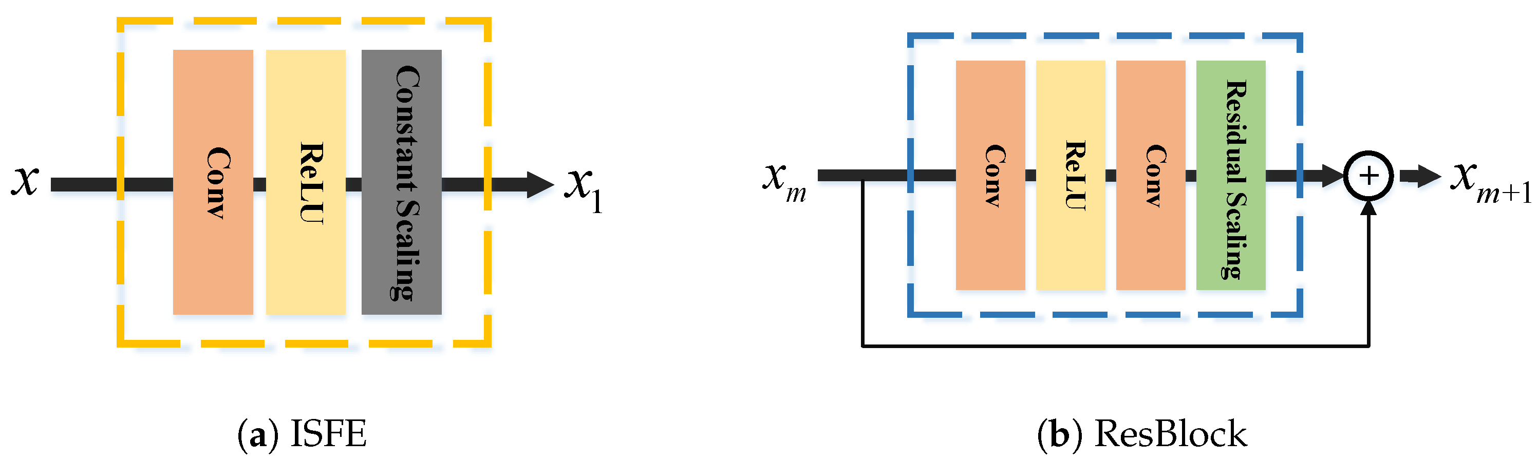
Within the SPRNet${}_{2\times }$ and SPRNet${}_{6\times }$, we can obtain numerous spectral feature maps which can contribute to the model performance. However, increasing the feature maps would lead to the unstable training procedure and destroy the sharpening results in return. To address this problem, we propose the ISFE unit with the structure in Figure 2a, which places a constant scaling layer after the convolution and activation function layers, to multiply the input features with a constant. With the input $\mathbf{x}$, they can be defined as:

$$\begin{array}{c}\hfill {\mathbf{x}}_1=\mu \phi \left(\mathbf{w}\ast \mathbf{x}+\mathbf{b}\right)\end{array}$$

(1)

where ${\mathbf{x}}_1$ denotes the output of ISFE, $\{\mathbf{w},\mathbf{b}\}$ means the weight matrix and basis of the convolution, $\phi$ is rectified linear unit (ReLU) as $\phi \left(x\right)=max\left(x,0\right)$, $\mu$ is the constant scaling with factor 0.05, and ∗ denotes the convolution operation.

To explore deeper spatial feature and learn the spatial mapping between LR and HR bands, the output of ISFE is fed to a series of ResBlocks with the structure in Figure 2b. Each Resblock consists of the convolution, activation function, and residual scaling layers [44]. To propagate the input information and alleviate the gradient vanishment problem, a skip-connection is added. So, the $m_{th}$ ResBlock can be computed as:

$$\left\{\begin{array}{c}{\mathbf{y}}_{m_1}=\phi \left({\mathbf{w}}_{m_1}\ast {\mathbf{x}}_m+{\mathbf{b}}_{m_1}\right)\hfill \\ {\mathbf{y}}_{m_2}=\lambda \left({\mathbf{w}}_{m_2}\ast {\mathbf{y}}_{m_1}+{\mathbf{b}}_{m_2}\right)\hfill \\ {\mathbf{x}}_{m+1}={\mathbf{x}}_m+{\mathbf{y}}_{m_2}\hfill \end{array}\right.$$

(2)

where ${\mathbf{y}}_{m_1}$ and ${\mathbf{y}}_{m_2}$ denote the intermediate results, $\{{\mathbf{w}}_m,{\mathbf{b}}_m\}$ is the weight matrix and basis of the convolution in Resblock, ${\mathbf{x}}_{m+1}$ denotes the output of the ResBlock, and $\lambda$ is a residual scaling with factor $0.1$.

2.3. Spatial Feature Fusing

In order to combine the information of different resolution bands, we propose the spatial feature fusing component. After the parallel residual learning component, the extracted feature maps learning from separate branches are concatenated so they can be simultaneously fed into the next layer. To fully fuse the information of these maps, two FC layers are adopted here and each of them is followed by a ReLU activation. Subsequently, a convolution layer is aimed to transform the feature maps into the spatial residual image with the channels as same as the sharpened bands. With the concatenated maps $\mathbf{z}$, these layers can be formulated as follows:

$$\left\{\begin{array}{c}{\mathbf{z}}_{f_1}=\phi \left({\mathbf{w}}_{f_1}\ast \mathbf{z}+{\mathbf{b}}_{f_1}\right)\hfill \\ {\mathbf{z}}_{f_2}=\phi \left({\mathbf{w}}_{f_2}\ast {\mathbf{z}}_{f_1}+{\mathbf{b}}_{f_2}\right)\hfill \\ {\mathbf{z}}_2={\mathbf{w}}_{f_3}\ast {\mathbf{z}}_{f_2}+{\mathbf{b}}_{f_3}\hfill \end{array}\right.$$

(3)

where ${\mathbf{z}}_f$ denotes the output of the FC layer, $\{{\mathbf{w}}_f,{\mathbf{b}}_f\}$ means the weight matrix and basis of the FC and convolution layers of this component, and ${\mathbf{z}}_2$ is the output. What’s more, after each convolutional operation, we adopt the zero padding to get the same size with the inputs.

2.4. Spectral Feature Mapping

The parallel spatial residual learning component and spatial feature fusing component mainly contribute toward learning the spatial mapping between the LR bands and targeted HR bands. Considering the target HR and input LR share the same spectral content, we construct the spectral feature mapping by adopting a skip-connection into the network to keep spectral consistency. This operation adds the up-scaled LR bands to the spatial residual image obtained from last step to propagate the spectral information directly. As such, the approximated HR can be produced by combining the spatial features and spectral characteristics.

2.5. Training and Applying

Following the above steps, the designed network can learn an end-to-end mapping between the LR and corresponding HR bands. However, due to the lack of HR reference, the mapping can not be learned from the data at original scale directly. It’s a generic solution that training and testing the sharpening methods follow Wald’s protocol [45] that takes the degraded data as inputs and the original data as the corresponding reference. This operation requires the base assumption that the mapping relationship between the LR and HR is scale-invariant (i.e., 40 m→20 m for inferring 20 m→10 m and 360 m→60 m for inferring 60 m→10 m). In this way, the image sharpening can be implemented using the degraded trained model. For convenience, the 10 m, 20 m and 60 m bands of Sentinel-2 data are denoted as ${\mathbf{X}}_{10}$, ${\mathbf{X}}_{20}$ and ${\mathbf{X}}_{60}$, respectively. And their degraded version which is convoluted with the predetermined point spread function (PSF) [23,27] and downsampled by utilizing bilinear interpolation, can be denoted as ${\mathbf{X}}_{10}^D$, ${\mathbf{X}}_{20}^D$ and ${\mathbf{X}}_{60}^D$, respectively. As mentioned before, it’s sufficient to train two networks SPRNet${}_{2\times }$ and SPRNet${}_{6\times }$. With the synthetic data pairs, these models can be trained as follows.

For SPRNet${}_{2\times }$, ${\mathbf{X}}_{10}^D$, ${\mathbf{X}}_{20}^D$ are created by downsampling the ${\mathbf{X}}_{10}$ and ${\mathbf{X}}_{20}$ by a factor 2, and used to train the 40 m→20 m network. Since the size of ${\mathbf{X}}_{10}^D$ and ${\mathbf{X}}_{20}^D$ is different, we can up-sample the ${\mathbf{X}}_{20}^D$ to the spatial size of ${\mathbf{X}}_{10}^D$. Then, we concatenate the ${\mathbf{X}}_{10}^D$ and up-sclaed ${\mathbf{X}}_{20}^D$ as the input of SPRNet${}_{\times 2}$. The mapping $F_{2\times }(·)$ can be learned by minimizing the loss between the HR reference ${\mathbf{X}}_{20}$ and the sharpening result $F_{2\times }([{\mathbf{X}}_{10}^D,{\mathbf{X}}_{20}^D],{\Theta }_1)$, where ${\Theta }_1$ is the model parameters, and the loss function can be formulated as follows:

$$\pounds \left({\Theta }_1\right)=\left|F_{2\times }([{\mathbf{X}}_{10}^D,{\mathbf{X}}_{20}^D],{\Theta }_1)-{\mathbf{X}}_{20}\right|$$

(4)

where $\left|·\right|$ denotes the L1-norm, which computes the mean absolute error between the generated and the reference data.

Compared with SPRNet${}_{2\times }$, the input and output of SPRNet${}_{6\times }$ are different. We downsample all bands by a factor 6. Then, we adopt the ${\mathbf{X}}_{10}^D$, ${\mathbf{X}}_{20}^D$ and ${\mathbf{X}}_{60}^D$ as input and the original ${\mathbf{X}}_{60}$ as HR reference to train the 360 m→60 m network. Like SPRNet${}_{2\times }$, this model is estimated by minimized the following loss function:

$$\pounds \left({\Theta }_2\right)=\left|F_{6\times }([{\mathbf{X}}_{10}^D,{\mathbf{X}}_{20}^D,{\mathbf{X}}_{60}^D],{\Theta }_2)-{\mathbf{X}}_{60}\right|$$

(5)

where ${\Theta }_2$ is the parameters of SPRNet${}_{6\times }$, and $F_{6\times }(·)$ denotes the mapping between ${\mathbf{X}}_{60}^D$ and ${\mathbf{X}}_{60}$.

On the basis of the above steps, the proposed method can learn the mapping between LR and HR bands. When we implement the image sharpening in the applying stage, we input the original bands X${}_{10}$, ${\mathbf{X}}_{20}$ and ${\mathbf{X}}_{60}$ to the trained SPRNet${}_{2\times }$ and SPRNet${}_{6\times }$ models to produce the estimated HR bands ${\mathbf{Y}}_{20}$ and ${\mathbf{Y}}_{60}$:

$$\begin{array}{cc}\hfill {\mathbf{Y}}_{20}& =F_{2\times }([{\mathbf{X}}_{10},{\mathbf{X}}_{20}],{\Theta }_1)\hfill \\ \hfill {\mathbf{Y}}_{60}& =F_{6\times }([{\mathbf{X}}_{10},{\mathbf{X}}_{20},{\mathbf{X}}_{60}],{\Theta }_2)\hfill \end{array}$$

(6)

The predicted ${\mathbf{Y}}_{20}$ and ${\mathbf{Y}}_{60}$ are the corresponding sharpening results at 10 m resolution of the 20 m and 60 m bands, respectively. Thus, the image with all bands at 10 resolution is obtained.

3. Experiments

3.1. Data

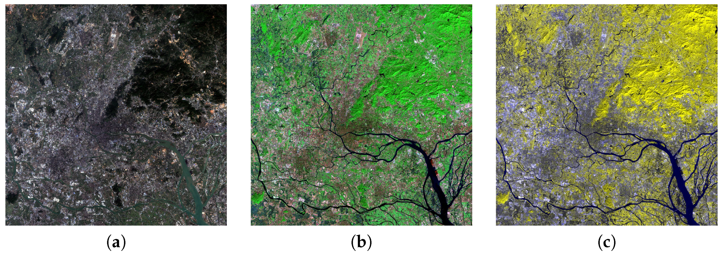
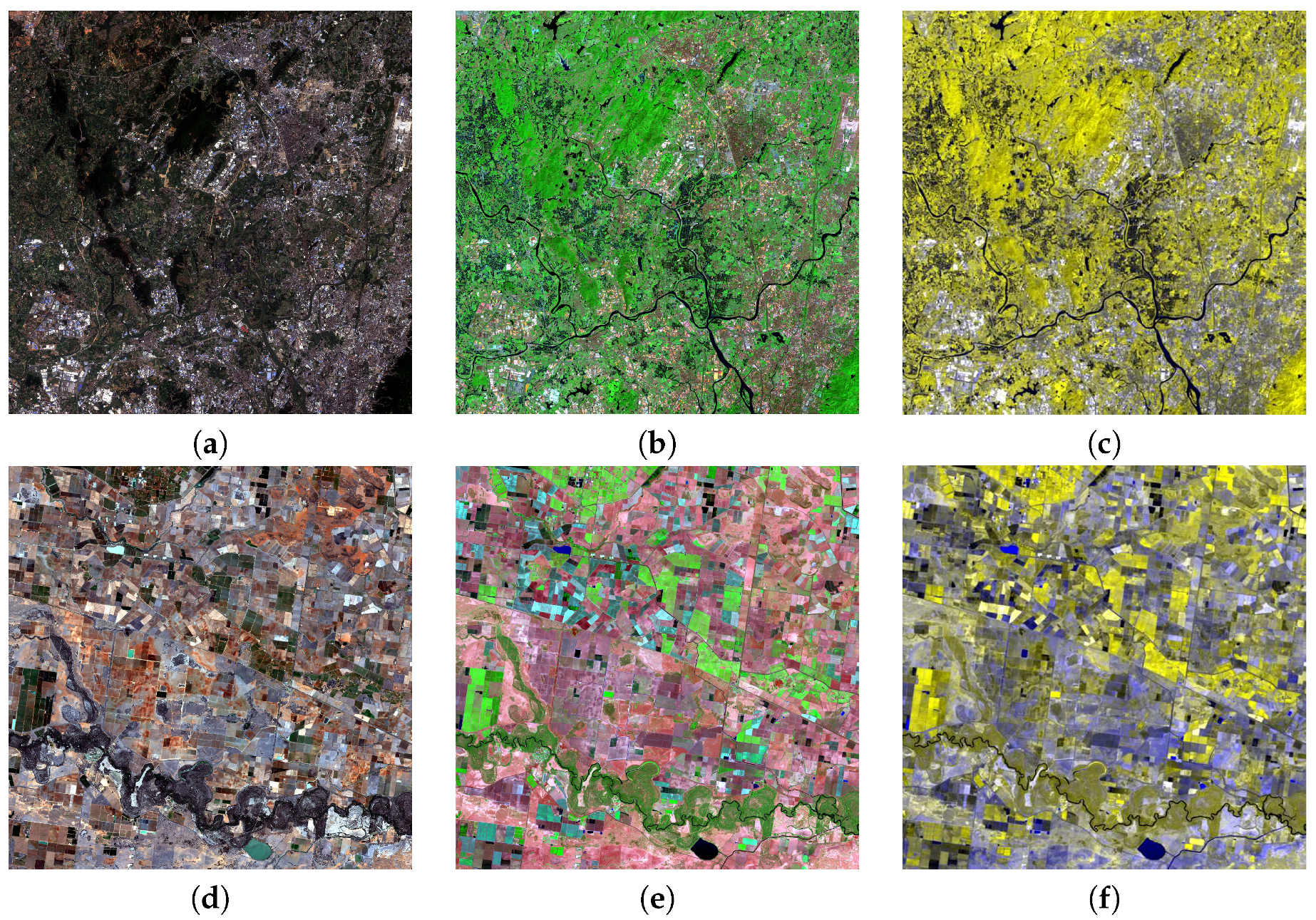
Our experimental data come from the Sentinel-2 Level-1C products, which have been converted from radiance into geo-coded top of atmosphere (TOA) reflectance with a sub-pixel multi-spectral registration [46]. The training data used in this paper cover a scene of Guangdong Province in China with a spatial extent of 72 km by 72 km and was collected on 31 December 2017. Figure 3 depicts the 10 m, 20 m and 60 m bands of this data. We adopt two datasets for testing. The first one covers a scene of Guangdong Province in China (site 1) and was obtained on 21 March 2018. The second one covers a scene of New South Wales in Australia (site 2) and was acquired on 4 December 2018. For each scene, we select an area with a spatial extent of 36 km by 36 km. The bands of the site 1 dataset are displayed in Figure 4a–c and those of the site 2 dataset are displayed in Figure 4d–f.

3.2. Experimental Details

In our experiments, some important parameters of the proposed method are configured as follows. To train the SPRNet${}_{2\times }$, the training data are degraded by a factor 2 and sliced to the patch of $60\times 60$ pixels. Similarly, to train the SPRNet${}_{6\times }$, the training data are degraded by a factor 6 and sliced to the patch of $20\times 20$ pixels. For each network, 3600 sample pairs can be used for training and $10\%$ of them are used for validation. The number of ResBlocks M is set as 6 in each branch and we use 128 filters of the size $3\times 3$ for convolution layers expect the last convolution in our evaluations. The choice of the parameter is inspired by [23]. Since the last convolution is aimed at reducing the feature dimension to the number of the sharpened bands, the number of filters is set as 6 and 2 in SPRNet${}_{2\times }$ and SPRNet${}_{6\times }$, respectively. These networks are implemented in the Keras framework with NVIDIA Tesla K80 GPU. We use the Nadam [47,48] with ${\beta }_1=0.9$, ${\beta }_1=0.999$ and $ϵ={10}^{-8}$ as optimizer to train the networks. The learning rate is initialized as ${10}^{-4}$, which can be reduced by a factor of 2 whenever the validation loss does not decrease for 5 epochs, and the reducing procedure is terminated whenever the learning rate is less than ${10}^{-5}$. The mini-batch size and the epoch number of training are set as 128 an 200, respectively.

3.3. Baselines and Quantitative Evaluation Metrics

To assess the effectiveness of our proposed method, we take SupReME [27], ResNet [43] and DSen2Net [23] as benchmark methods. Besides, the bicubic interpolation (Bicubic) is used to illustrate the performance of the naive upsampling without considering spectral correlations. The parameters of SupReME and DSen2Net are set as suggested in the original publications, while the number of ResBlocks in ResNet is set as 6.

We adopt six evaluation metrics for quantitative evaluation including: root mean squared error (RMSE), signal-to-reconstruction error (SRE), correlation coefficient (CC), universal image quality index (UIQI), $erreur$ $relative$ $globale$ $adimensionnelle$ $de$ $synth\stackrel{‵}{e}se$ (ERGAS) and spectral angle mapper (SAM) [45,49]. The RMSE and SRE evaluate the quantitative similarity between the target images and the reference images based on mean square error (MSE). The CC indicates the correlation and the UIQI is a mathematically defined universal image quality index, which can be applied to various image processing applications. The ERGAS reflects fidelity of the target images based on the weighted sum of MSE in each band, and the SAM describes the spectral fidelity of the sharpening results. In these evaluation metrics, when the sharpening results are closer to the reference one, the values of RMSE, ERGAS, and SAM are smaller, on the contrary, the values of SRE, CC, and UIQI are larger.

3.4. Experimental Results

3.4.1. Evaluation at Lower Scale

Since the 10 m version of LR bands are not available in the testing datasets, we follow the Wald’s protocol and give the quantitative evaluation at lower scale, i.e., the SPRNet${}_{2\times }$ is evaluated on the task to sharpen 40 m to 20 m; in the same way, the SPRNet${}_{6\times }$ is evaluated on the task to sharpen 360 m to 60 m. The lower scale data are generated by synthetically degrading the original data by the upscale ratio (i.e., 2 for SPRNet${}_{2\times }$ and 6 for SPRNet${}_{6\times }$). In the following, we separately discuss the effectiveness of the SPRNet${}_{2\times }$ and SPRNet${}_{6\times }$.

SPRNet${}_{\mathbf{2}\mathbf{\times }}$—20 m bands. As for 20 m bands sharpening, the network SPRNet${}_{2\times }$ is trained by the simulated data degraded from the observed data by a factor 2 to learn the mapping between 40 m and 20 m. Several state-of-the-art methods are compared with the proposed method.

Table 2. Quantitative assessment of the SPRNet${}_{2\times }$ at lower scale (input 40 m, output 20 m) on site 1. Bold indicates the best performance.

	Ideal	Band	Bicubic	SupReME	ResNet	DSen2Net	SPRNet
RMSE	0	B5	172.571	121.093	59.363	50.719	44.007
		B6	227.449	156.636	81.834	66.152	56.708
		B7	262.031	160.877	83.242	70.331	60.983
		B8a	289.247	175.351	89.080	72.175	62.439
		B11	238.489	182.597	95.896	76.858	60.541
		B12	236.283	189.993	108.664	98.661	74.780
		Mean	237.678	164.424	86.347	72.483	59.910
SRE (dB)	∞	B5	18.443	21.454	27.716	29.051	30.213
		B6	18.899	22.034	27.632	29.501	30.776
		B7	18.634	22.852	28.425	29.980	31.199
		B8a	18.187	22.550	28.343	30.177	31.451
		B11	17.899	19.943	25.623	27.541	29.475
		B12	15.483	17.152	22.118	22.847	25.212
		Mean	17.924	20.998	26.643	28.183	29.721
CC	1	B5	0.916	0.959	0.990	0.993	0.995
		B6	0.888	0.947	0.986	0.991	0.993
		B7	0.889	0.959	0.989	0.992	0.994
		B8a	0.894	0.962	0.990	0.994	0.995
		B11	0.930	0.958	0.989	0.993	0.996
		B12	0.933	0.956	0.986	0.989	0.993
		Mean	0.908	0.957	0.988	0.992	0.994
UIQI	1	B5	0.695	0.874	0.961	0.971	0.978
		B6	0.669	0.881	0.961	0.974	0.980
		B7	0.673	0.900	0.970	0.978	0.983
		B8a	0.678	0.903	0.971	0.981	0.985
		B11	0.724	0.870	0.956	0.970	0.980
		B12	0.720	0.855	0.952	0.960	0.974
		Mean	0.693	0.881	0.962	0.972	0.980
ERGAS	0		2.262	1.636	0.879	0.756	0.606
SAM	0		2.845	2.347	2.006	1.666	1.384

and

Table 3. Quantitative assessment of the SPRNet${}_{2\times }$ at lower scale (input 40 m, output 20 m) on site 2. Bold indicates the best performance.

	Ideal	Band	Bicubic	SupReME	ResNet	DSen2Net	SPRNet
RMSE	0	B5	93.332	58.979	44.042	35.161	25.443
		B6	100.533	65.210	53.416	43.207	26.161
		B7	114.797	70.440	62.458	49.627	28.337
		B8a	128.315	77.231	72.154	48.098	30.561
		B11	176.907	135.533	102.824	90.342	53.017
		B12	165.544	138.220	91.405	80.193	51.161
		Mean	129.905	90.935	71.050	57.771	35.780
SRE (dB)	∞	B5	25.366	29.386	31.694	33.761	36.636
		B6	26.286	29.999	31.630	33.584	37.922
		B7	26.190	30.376	31.403	33.417	38.295
		B8a	26.151	30.564	31.116	34.635	38.612
		B11	25.477	27.309	30.034	31.145	35.849
		B12	23.752	24.680	28.745	29.918	33.740
		Mean	25.537	28.719	30.770	32.744	36.842
CC	1	B5	0.964	0.986	0.992	0.995	0.997
		B6	0.964	0.985	0.990	0.994	0.998
		B7	0.968	0.988	0.991	0.994	0.998
		B8a	0.968	0.989	0.991	0.996	0.998
		B11	0.974	0.984	0.992	0.993	0.998
		B12	0.976	0.983	0.993	0.994	0.998
		Mean	0.969	0.986	0.991	0.994	0.998
UIQI	1	B5	0.750	0.915	0.936	0.956	0.975
		B6	0.748	0.911	0.924	0.947	0.975
		B7	0.752	0.920	0.922	0.947	0.977
		B8a	0.752	0.919	0.924	0.955	0.977
		B11	0.763	0.880	0.900	0.921	0.966
		B12	0.768	0.866	0.901	0.924	0.960
		Mean	0.755	0.902	0.918	0.942	0.972
ERGAS	0		0.893	0.637	0.486	0.398	0.249
SAM	0		1.173	1.071	1.239	0.945	0.586

list the quantitative assessment results of these methods for two testing datasets. Among them, we calculate RMSE, SRE, CC, UIQI on each band, and then compute the mean values over the bands. The ideal value of each index is provided for the convenience of inter-comparison. The best results are highlighted in bold.

According to the reported results, a few observations are noteworthy. (1) All the methods are significantly better than the Bicubic method, especially the CNN-based methods, which outperform the Bicubic by a large margin. For instance, our SPRNet reduces the RMSE by a factor of above 2 and reaches more than 10 dB higher SRE. This illustrates the effectiveness of the sharpening procedure. (2) The proposed SPRNet method obtains the best evaluation results in all indexes. For site 1, the mean RMSE of the SPRNet is 59.910, with a decrease of 104.514, 26.437 and 12.573 when compared to SupReME, ResNet and DSen2Net. Accordingly, the mean SRE value of the SPRNet is 29.721 dB, which is 8.723 dB, 3.078 dB and 1.538 dB higher than that of the aforesaid methods, respectively. Also, the mean CC and UIQI of the SPRNet are 0.994 and 0.980 with gains of 0.002 and 0.008 over that of the best comparison method DSen2Net. For site 2, the mean RMSE of the SPRNet is 55.155, 35.27 and 21.991 smaller than that of SupReME, ResNet and DSen2Net, respectively. And the mean SRE is 8.123 dB, 6.072 dB and 4.098 dB higher than that of the corresponding methods, respectively. Compared with the DSen2Net, the mean CC and UIQI of the SPRNet increase by 0.004 and 0.03. The above results demonstrate the great spatial similarity of the proposed SPRNet. Moreover, we also observe the proposed method obtains the best ERGAS and SAM. The ERGAS of the SPRNet for two sites are 0.273 and 0.237 lower than that of the ResNet, while 0.15 and 0.149 lower than that of the DSen2Net. The SAM of the SPRNet for site 1 is 1.384 while that of the compared methods are larger than 1.6 and the SAM of the SPRNet for site 2 is 0.586 while that of the competitors are higher than 0.9. These analyses indicate the effectiveness of our SPRNet in both spatial and spectral domains.

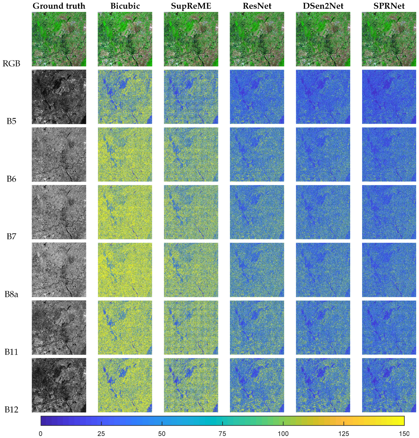
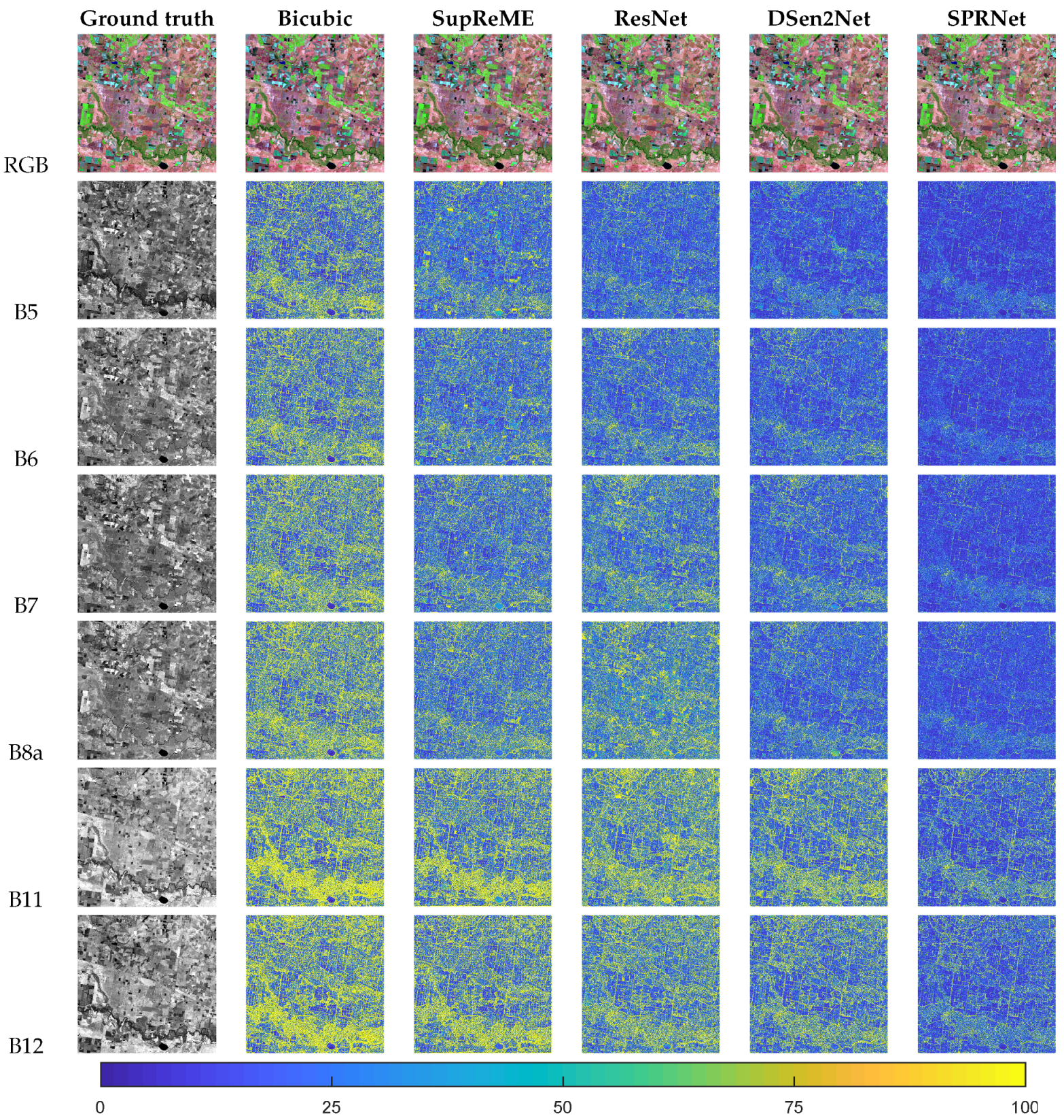
Furthermore, we depict visual comparisons with different methods on two testing datasets in Figure 5 and Figure 6. The figures provide the RGB (B12, B8a and B5 as RGB) and each bands results. In order to observe the difference between sharpening results and ground truth clearly, the absolute differences between them are presented. In these figures, if the sharpening results are either blur edges or exaggerate the contrast, the residual errors are high, on the contrary, when the results are similar to the ground truth, the residual errors trend to zero. It can be seen that the results of SPRNet are closer to the reference while the compared methods exhibit errors along high contrast edges at almost bands. In Figure 5, the images of the Bicubic and SupReME are more bright, meaning these methods get deteriorate results for the spatial reconstruction. In contrast, the CNN-based methods have more smooth regions with dark color and the edges of structures are less, and the best results can be found in the SPRNet. As for Figure 6, the boundaries of the land plots are still obvious in the Bicubic and SupReME. Among the CNN-based methods, SPRNet performs satisfactorily, especially for B5, B6, B7 and B8a.

SPRNet${}_{\mathbf{6}\mathbf{\times }}$—60 m bands. To sharpen the 60 m bands, we train another network SPRNet${}_{6\times }$ using downgraded data with resolution 60 m, 120 m and 360 m to learn the mapping from 360 m to 60 m. The quantitative results of site 1 and site 2 are shown in

Table 4. Quantitative assessment of the SPRNet${}_{6\times }$ at lower scale (input 360 m, output 60 m) on site 1. Bold indicates the best performance.

	Ideal	Band	Bicubic	SupReME	ResNet	DSen2Net	SPRNet
RMSE	0	B1	139.703	53.456	51.702	38.833	23.473
		B9	137.938	50.511	35.213	30.847	24.437
		Mean	138.821	51.984	43.457	34.840	23.955
SRE (dB)	∞	B1	20.855	29.319	29.674	32.086	36.446
		B9	15.728	24.300	27.672	28.746	30.762
		Mean	18.292	26.810	28.673	30.416	33.604
CC	1	B1	0.802	0.973	0.975	0.988	0.995
		B9	0.681	0.962	0.982	0.988	0.991
		Mean	0.742	0.968	0.979	0.988	0.993
UIQI	1	B1	0.234	0.870	0.866	0.940	0.978
		B9	0.175	0.929	0.964	0.971	0.981
		Mean	0.205	0.900	0.915	0.955	0.980
ERGAS	0		2.167	0.807	0.622	0.515	0.381
SAM	0		3.039	1.228	0.937	0.704	0.542

and

Table 5. Quantitative assessment of the SPRNet${}_{6\times }$ at lower scale (input 360 m, output 60 m) on site 2. Bold indicates the best performance.

	Ideal	Band	Bicubic	SupReME	ResNet	DSen2Net	SPRNet
RMSE	0	B1	64.444	34.835	35.902	24.026	14.919
		B9	72.906	27.764	22.113	18.561	12.750
		Mean	68.675	31.299	29.007	21.293	13.835
SRE (dB)	∞	B1	26.281	30.884	31.758	34.707	38.938
		B9	20.569	28.971	30.608	32.268	35.546
		Mean	23.425	29.928	31.183	33.488	37.242
CC	1	B1	0.850	0.960	0.956	0.981	0.992
		B9	0.853	0.980	0.987	0.991	0.996
		Mean	0.852	0.970	0.971	0.986	0.994
UIQI	1	B1	0.348	0.895	0.852	0.919	0.965
		B9	0.344	0.936	0.948	0.963	0.980
		Mean	0.346	0.916	0.900	0.941	0.972
ERGAS	0		1.203	0.503	0.442	0.341	0.227
SAM	0		1.521	0.728	0.659	0.504	0.342

, respectively. Once again, the advantage of the proposed SPRNet over the competing methods is obvious. For site 1, the mean RMSE of SPRNet is 114.866, 28.029, 19.502 and 10.885 smaller than that of Bicubic, SupReME, ResNet and DSen2Net, respectively. And the mean SRE of SPRNet is 15.312 dB, 6.794 dB, 4.931 dB and 3.188 dB higher than the corresponding methods. Compared with the DSen2Net, the mean CC and UIQI of the SPRNet increase by 0.005 and 0.025, while the ERGAS and SAM decrease by 0.134 and 0.162. For site 2, when compared to Bicubic, SupReME, ResNet and DSen2Net, the mean RMSE of SPRNet is 13.835, with a decrease of 54.84, 17.464, 15.172 and 7.458 while the mean SRE of SPRNet increases by 13.817 dB, 7.314 dB, 6.059 dB, 3.754 dB. The mean CC and UIQI of the SPRNet are 0.994 and 0.972, with gains of 0.008 and 0.031 over that of the DSen2Net. In addition, the ERGAS and SAM of the SPRNet are 0.114 and 0.162 smaller than that of the DSen2Net. These results reveal the effectiveness of the SPRNet in sharpening 60m bands, which further show feasibility and suitability of the proposed method.

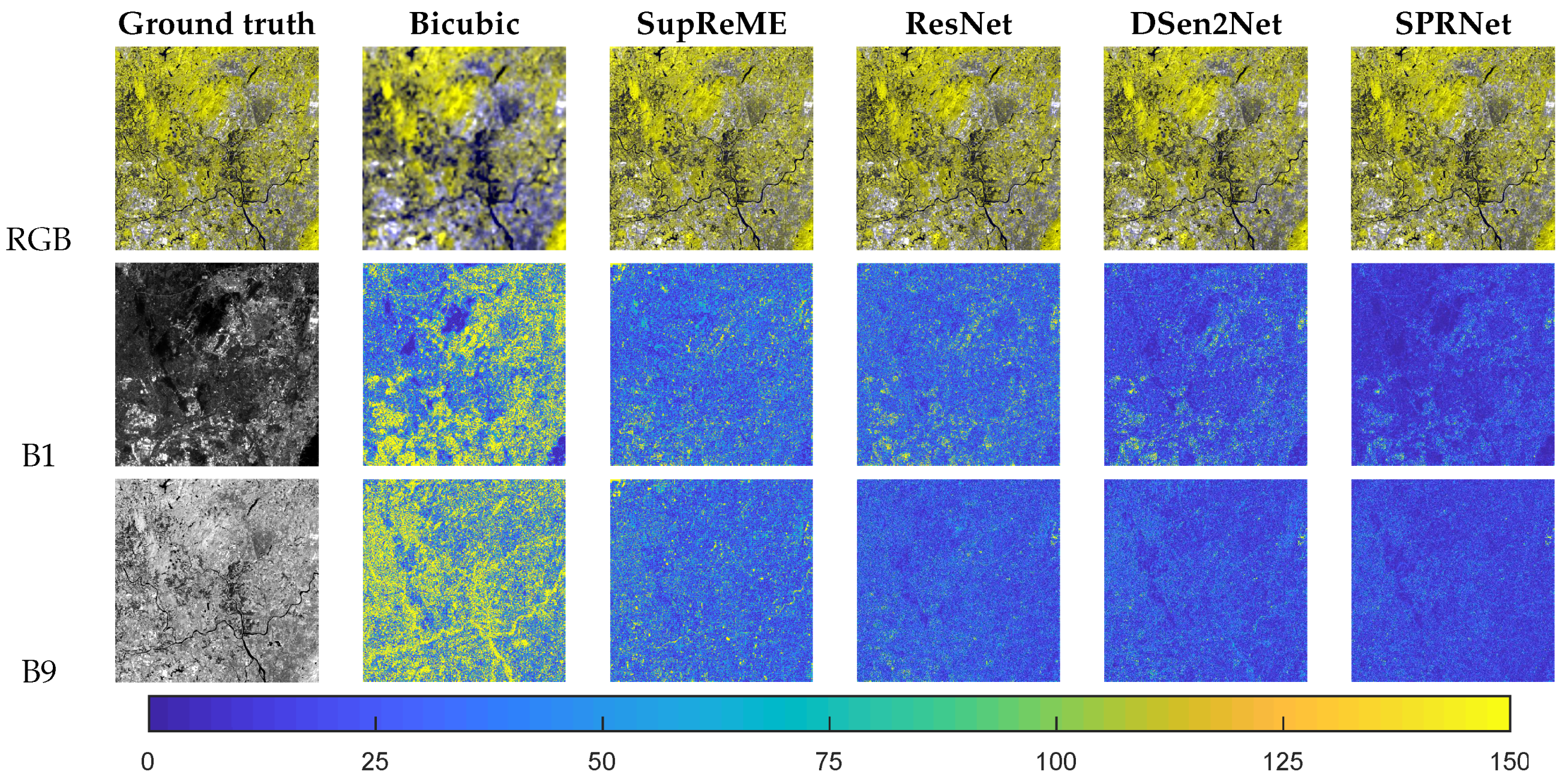
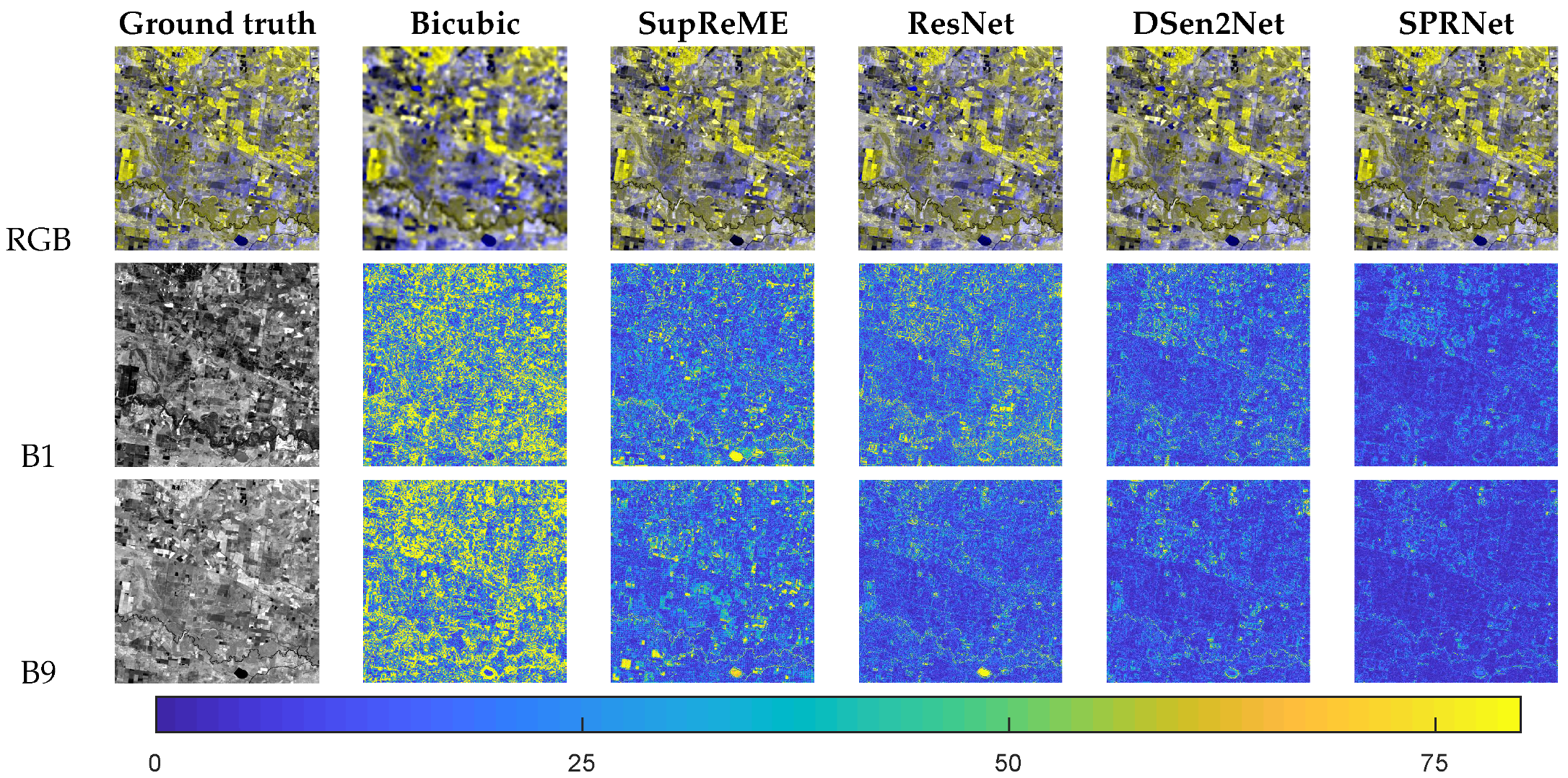
We also perform a qualitative comparison to ground truth. The RGB (B9, B9 and B1 as RGB) results and absolute residuals of two sites are plotted in Figure 7 and Figure 8. The visual impression of 60 m bands confirms that the SPRNet clearly dominates the competition with much less structured residuals. We can observe that the competing methods have more residuals for both sites, in contrast, the results of our method have more smooth regions and the color is prone to dark. This indicates our method obtains the best overall performance.

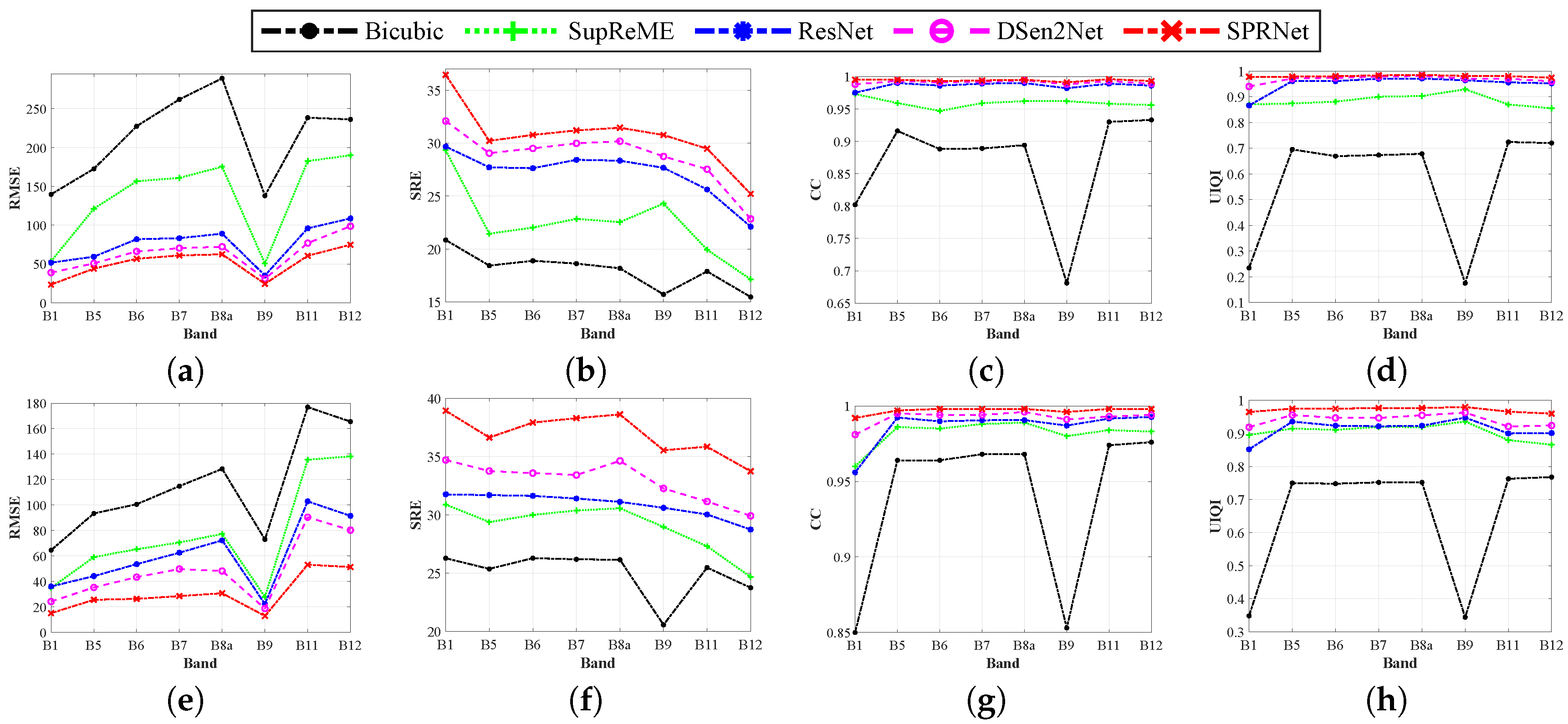
The performance of different bands. To verify the generic ability of the sharpening methods on different spectral wavelengths, the performance curves of different bands for different indices are shown in Figure 9. Almost all methods show the similar trend and the performance of the CNN-based methods are substantially better. Among the 20 m bands (i.e., B5, B6, B7, B8a, B11 and B12), we find that all the methods exhibit a marked drop in accuracy of B11 and B12. The numeric comparisons can be found in Table 2 and Table 3. For instance, compared to the average level, the SRE values of SPRNet drop 0.246 dB (site 1) and 0.993 dB (site 2) on B11, while drop 4.509 dB (site 1) and 3.102 dB (site 2) on B12. The reason is that these two bands lie in the SWIR spectrum (>1600 nm), which beyond the spectral range (400∼900 nm) of 10 m resolution bands, and thus the details of B11 and B12 can not be infer exactly by borrowing the 10 m information. As for the 60 m bands (i.e., B1 and B9), the accuracy of the Bicubic is obviously lower than other methods. This is due to the fact that the Bicubic can not use any information from the auxiliary HR bands, which aggravates the difficulties of recovering the details. Furthermore, the performance of B9 is slightly worse than that of B1. Since the center wavelength of B1 is 443 nm which is covered by 400∼900 nm, but B9 (center wavelength at 945 nm) is out of this range, the useful information borrowed from 10 m bands is limited. These observations indicate that the bands closer to the auxiliary HR bands can have more precise sharpening results.

3.4.2. Evaluation at the Original Scale

To verify the generalization of our method to true scale Sentinel-2 data, we directly feed the original LR and 10 m bands into the trained networks (i.e., band sets [20 m, 10 m] fed into SPRNet${}_{2\times }$ and band sets [60 m, 20 m, 60 m] fed into SPRNet${}_{6\times }$) to produce 10 m resolution version of the LR bands.As there is no ground truth being present, the higher resolution spectral bands are considered as the reference data to assess the sharpening method. In our experiments, four spectral bands with 10 m resolution are served as the reference data for visual evaluation. The up-scaled results of a sub-area obtained by the Bicubic and SPRNet are shown in Figure 10 and Figure 11.

From these figures, we can clearly observe that the sharpening results of the SPRNet receive a good visual quality. Although the bicubic interpolation has properties of smoothing the original images, it is unable to recover the spatial details, while the sharpening results of the SPRNet are sharper and bring out additional details in all cases. Moreover, we can find that the sharpening results of LR bands improve the spatial resolution without noticeable artifacts. To be specific, as can be observed from the marked region (red rectangle), the SPRNet produces much sharper edges and the details of ground object are more abundant. In Figure 10, compared with the 10 m bands, the original 20 m bands can not show the outlines of the building clearly and the original 60 m bands are difficult to depict the subject. Nevertheless, our method commendably enhances the spatial resolution of 20 m and 60 m bands and recovers the details of the building in these bands. In Figure 11, the contours are clear and vivid in the sharpening results of the SPRNet whereas they are blurred or distorted in the original LR data. What’s more, the sharpening results of LR bands match the 10 m resolution bands. These observations further imply our SPRNet can effectively sharpen the Sentinel-2 images and obtain a complete data at 10 m resolution.

4. Discussions

4.1. Effect of Combining Various-Resolution Bands

To investigate the impacts of fusing various-resolution bands, we test different combinations of 10 m, 20 m, and 60 m band sets as the input to the SPRNet${}_{\mathbf{2}\times }$ and SPRNet${}_{\mathbf{6}\times }$. The experiment results of two testing data are displayed in

Table 6. The comparison results of the SPRNet with different combination of 10 m, 20 m and 60 m band sets.

Model	SPRNet${}_{2\times }$			SPRNet${}_{6\times }$
	SPRNet${}_{2\times }$-1	SPRNet${}_{2\times }$-2	SPRNet${}_{2\times }$-3	SPRNet${}_{6\times }$-1	SPRNet${}_{6\times }$-2	SPRNet${}_{6\times }$-3
10 m	✗	✓	✓	✗	✓	✓
20 m	✓	✓	✓	✗	✗	✓
60 m	✗	✗	✓	✓	✓	✓
RMSE	144.934/85.833	59.910/35.780	67.260/40.917	131.115/62.107	27.021/17.578	23.955/13.835
SRE	21.939/28.895	29.721/36.842	28.810/36.074	18.772/24.220	32.616/35.155	33.604/37.242
CC	0.965/0.986	0.994/0.998	0.993/0.997	0.772/0.875	0.991/0.990	0.993/0.994
UIQI	0.889/0.878	0.980/0.972	0.976/0.964	0.299/0.444	0.973/0.958	0.980/0.972
ERGAS	1.356/0.594	0.606/0.249	0.698/0.291	2.038/1.082	0.425/0.289	0.381/0.227
SAM	2.022/0.987	1.384/0.586	1.539/0.685	2.812/1.342	0.609/0.419	0.542/0.342

The values before “/” are the results of site 1, while the values after “/” are the results of site 2.

. As for the SPRNet${}_{\mathbf{2}\times }$, we take the model trained by the 20 m set as the baseline (SPRNet${}_{2\times }$-1). We then add the 10 m set to the SPRNet${}_{2\times }$-1, resulting in SPRNet${}_{2\times }$-2. From the SPRNet${}_{2\times }$-1 to SPRNet${}_{2\times }$-2, the SRE values increase by 7.782 dB for site 1 and 7.947 dB for site 2, which demonstrates the effectiveness of utilizing the information from the 10 m bands to enhance the 20 m bands. We further add the 60 m set to the SPRNet${}_{2\times }$-2, resulting in SPRNet${}_{2\times }$-3. Compared with the SPRNet${}_{2\times }$-2, the SRE values of the SPRNet${}_{2\times }$-3 decrease by 0.911 dB and 0.768 dB for site 1 and site 2, respectively. This is because that the lower resolution bands can not contribute to higher resolution bands sharpening. As for the SPRNet${}_{\mathbf{6}\times }$, the baseline (SPRNet${}_{6\times }$-1) is only trained by the 60 m set. Due to the large amplification factor, the SPRNet${}_{\mathbf{6}\times }$-1 can not learn the LR and HR mapping accurately. The SPRNet${}_{6\times }$-2 is obtained by adding the 10 m set to the SPRNet${}_{6\times }$-1. The SRE values of the SPRNet${}_{6\times }$-2 are 13.844 dB and 10.935 dB higher than that of the SPRNet${}_{6\times }$-1 for site 1 and stie 2, respectively. Moreover, the SPRNet${}_{6\times }$-3 combining the 10 m, 20 m and 60 m sets outperform other models, which implies that both 10 m and 20 m bands provide useful information to reproduce the details of 60 m bands. Based on the above analysis, we draw the conclusion that auxiliary bands with finer resolution can efficiently improve the sharpening results. Therefore, it is reasonable to sharpen Sentinel-2 image using two separate networks with different inputs.

4.2. Effect of Constant Scaling in ISFE

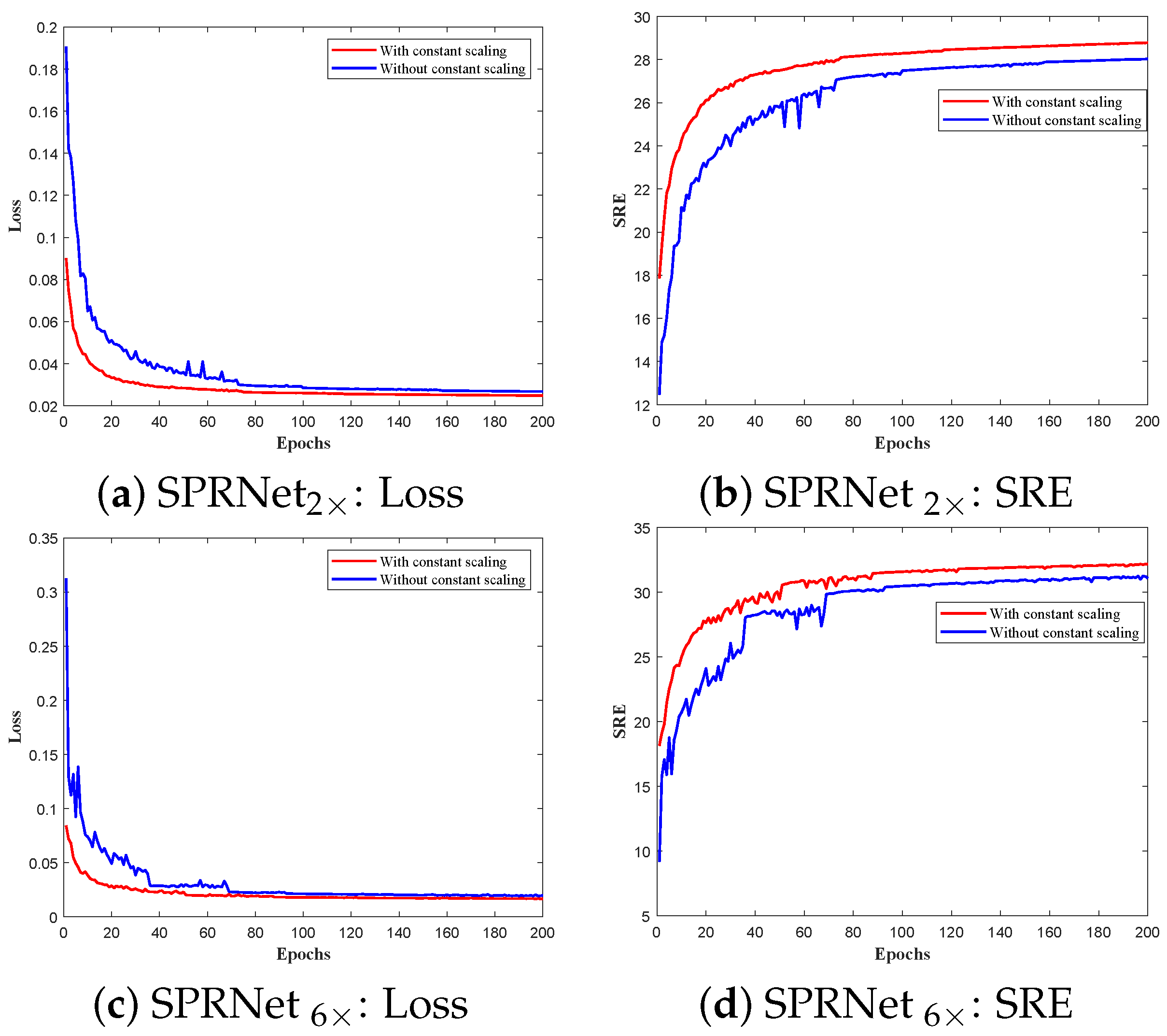
To investigate the effects of the constant scaling in ISFE unit, we display the training curves of our proposed method with and without constant scaling, and the speed of the training procedure is displayed in Figure 12, from which two observations can be drawn. First, we find that the networks with constant scaling converge faster. As for the SPRNet${}_{2\times }$, the network with constant scaling converges rapidly to the fine performance during 80 epochs, while the network without constant scaling takes about 100 epochs to reach the maximum performance. As for the SPRNet${}_{6\times }$, the learning loss of the network with constant scaling tends to stable before 60 epochs, but the margin fluctuation of another curve becomes smaller until 70 epochs. Second, the final accuracy is higher for the networks with constant scaling. Compared with the networks without constant scaling, the SRE values of the networks with constant scaling are increase by more than 5 dB at the first epoch. Even if the training epochs reach to 200, the SRE values of the networks without constant scaling are still lower than that of the proposed networks. Therefore, the addition of constant scaling is a simple but powerful strategy in our SPRNet.

5. Conclusions

In this paper, we propose a parallel residual network (i.e., SPRNet) for Sentinel-2 image sharpening to obtain complete data at the highest sensor resolution. The proposed method is designed to sharpen both 20 m and 60 m bands. Compared with existing deep learning-based methods, the main advantage of our SPRNet is that the sufficient spatial information of different resolution bands are extracted by separate branches in a parallel structure. In addition, the spatial information fusing and spectral characteristics propagating can be presented by the designed spatial feature fusing component and spectral feature mapping component. As such, the proposed method obtains the good sharpening results in the spatial fidelity and the spectral preservation. By learning the LR and corresponding HR mapping at lower scale, the trained SPRNet can produce the image at 10 m resolution with the original Sentinel-2 data. Extensive experiments on the degraded and original data prove the proposed method is competitive with the state-of-the-art approaches. In quantitative evaluations on the degraded data, for 20 m bands, the SRE of the SPRNet is 1.538 dB (site 1) and 4.098 dB (site 2) higher than the best competing approach; for 60 m bands, the SPRNet increases the SRE by 3.188 dB (site 1) and 3.754 dB (site 2) compared to the best competing approach. The proposed method also shows visually convincing results on original data. In the future, we will discuss the effects of the network parameters and try to adaptively decide the parameters. How to apply the sharpening results to other application areas (e.g., target detection and classification) is also a future research topic.

References

- Schmitt, M.; Hughes, L.H.; Zhu, X.X. The SEN1-2 Dataset for Deep Learning in SAR-Optical Data Fusion. arXiv 2018, arXiv:1807.01569. [Google Scholar] [CrossRef] [Green Version]
- Frampton, W.J.; Dash, J.; Watmough, G.; Milton, E.J. Evaluating the capabilities of Sentinel-2 for quantitative estimation of biophysical variables in vegetation. ISPRS J. Photogramm. Remote Sens. 2013, 82, 83–92. [Google Scholar] [CrossRef] [Green Version]
- Castillo, J.A.A.; Apan, A.A.; Maraseni, T.N.; Salmo, S.G., III. Estimation and mapping of above-ground biomass of mangrove forests and their replacement land uses in the Philippines using Sentinel imagery. ISPRS J. Photogramm. Remote Sens. 2017, 134, 70–85. [Google Scholar] [CrossRef]
- Delloye, C.; Weiss, M.; Defourny, P. Retrieval of the canopy chlorophyll content from Sentinel-2 spectral bands to estimate nitrogen uptake in intensive winter wheat cropping systems. Remote Sens. Environ. 2018, 216, 245–261. [Google Scholar] [CrossRef]
- Mura, M.; Bottalico, F.; Giannetti, F.; Bertani, R.; Giannini, R.; Mancini, M.; Orlandini, S.; Travaglini, D.; Chirici, G. Exploiting the capabilities of the Sentinel-2 multi spectral instrument for predicting growing stock volume in forest ecosystems. Int. J. Appl. Earth Obs. Geoinf. 2018, 66, 126–134. [Google Scholar] [CrossRef]
- Vrabel, J. Multispectral imagery band sharpening study. Photogramm. Eng. Remote Sens. 1996, 62, 1075–1084. [Google Scholar]
- Matteoli, S.; Diani, M.; Corsini, G. Automatic target recognition within anomalous regions of interest in hyperspectral images. IEEE J. Sel. Top. Appl. Earth Obs. Remote Sens. 2018, 11, 1056–1069. [Google Scholar] [CrossRef]
- Murray, N.J.; Keith, D.A.; Simpson, D.; Wilshire, J.H.; Lucas, R.M. REMAP: An online remote sensing application for land cover classification and monitoring. Methods. Ecol. Evol. 2018, 9, 2019–2027. [Google Scholar] [CrossRef] [Green Version]
- Liu, Z.; Li, G.; Mercier, G.; He, Y.; Pan, Q. Change detection in heterogenous remote sensing images via homogeneous pixel transformation. IEEE Trans. Image Process. 2017, 27, 1822–1834. [Google Scholar] [CrossRef]
- Sirguey, P.; Mathieu, R.; Arnaud, Y.; Khan, M.M.; Chanussot, J. Improving MODIS spatial resolution for snow mapping using wavelet fusion and ARSIS concept. IEEE Geosci. Remote Sens. Lett. 2008, 5, 78–82. [Google Scholar] [CrossRef] [Green Version]
- Aiazzi, B.; Alparone, L.; Baronti, S.; Santurri, L.; Selva, M. Spatial resolution enhancement of ASTER thermal bands. In Image Signal Processing Remote Sensing XI; International Society for Optics and Photonics: Bellingham, WA, USA, 2005; Volume 5982, p. 59821G. [Google Scholar]
- Maglione, P.; Parente, C.; Vallario, A. Pan-sharpening Worldview-2: IHS, Brovey and Zhang methods in comparison. Int. J. Eng. Technol 2016, 8, 673–679. [Google Scholar]
- Picaro, G.; Addesso, P.; Restaino, R.; Vivone, G.; Picone, D.; Dalla Mura, M. Thermal sharpening of VIIRS data. In Proceedings of the 2016 IEEE International Geoscience and Remote Sensing Symposium (IGARSS), Beijing, China, 10–15 July 2016; pp. 7260–7263. [Google Scholar]
- Carper, W.; Lillesand, T.; Kiefer, R. The use of intensity-hue-saturation transformations for merging SPOT panchromatic and multispectral image data. Photogramm. Eng. Remote Sens. 1990, 56, 459–467. [Google Scholar]
- Aiazzi, B.; Baronti, S.; Selva, M. Improving component substitution pansharpening through multivariate regression of MS + Pan data. IEEE Trans. Geosci. Remote Sens. 2007, 45, 3230–3239. [Google Scholar] [CrossRef]
- Shensa, M.J. The discrete wavelet transform: Wedding the à trous and Mallat algorithms. IEEE Trans. Signal Process. 1992, 40, 2464–2482. [Google Scholar] [CrossRef] [Green Version]
- Wang, Q.; Shi, W.; Li, Z.; Atkinson, P.M. Fusion of Sentinel-2 images. Remote Sens. Environ. 2016, 187, 241–252. [Google Scholar] [CrossRef] [Green Version]
- Vaiopoulos, A.; Karantzalos, K. Pansharpening on the narrow VNIR and SWIR spectral bands of Sentinel-2. Int. Arch. Photogramm. Remote Sens. Spat. Inf. Sci. 2016, 41, 723. [Google Scholar] [CrossRef]
- Park, H.; Choi, J.; Park, N.; Choi, S. Sharpening the VNIR and SWIR bands of Sentinel-2A imagery through modified selected and synthesized band schemes. Remote Sens. 2017, 9, 1080. [Google Scholar] [CrossRef] [Green Version]
- Kaplan, G. Sentinel-2 Pan Sharpening-Comparative Analysis. MDPI Proc. 2018, 2, 345. [Google Scholar] [CrossRef] [Green Version]
- Du, Y.; Zhang, Y.; Ling, F.; Wang, Q.; Li, W.; Li, X. Water bodies’ mapping from Sentinel-2 imagery with modified normalized difference water index at 10-m spatial resolution produced by sharpening the SWIR band. Remote Sens. 2016, 8, 354. [Google Scholar] [CrossRef] [Green Version]
- Gašparović, M.; Jogun, T. The effect of fusing Sentinel-2 bands on land-cover classification. Int. J. Remote Sens. 2018, 39, 822–841. [Google Scholar] [CrossRef]
- Lanaras, C.; Bioucas-Dias, J.; Galliani, S.; Baltsavias, E.; Schindler, K. Super-resolution of Sentinel-2 images: Learning a globally applicable deep neural network. ISPRS J. Photogramm. Remote Sens. 2018, 146, 305–319. [Google Scholar] [CrossRef] [Green Version]
- Simões, M.; Bioucas-Dias, J.; Almeida, L.B.; Chanussot, J. A convex formulation for hyperspectral image superresolution via subspace-based regularization. IEEE Trans. Geosci. Remote Sens. 2014, 53, 3373–3388. [Google Scholar] [CrossRef] [Green Version]
- Khademi, G.; Ghassemian, H. Incorporating an adaptive image prior model into Bayesian fusion of multispectral and panchromatic images. IEEE Geosci. Remote Sens. Lett. 2018, 15, 917–921. [Google Scholar] [CrossRef]
- Cheng, M.; Wang, C.; Li, J. Sparse representation based pansharpening using trained dictionary. IEEE Geosci. Remote Sens. Lett. 2013, 11, 293–297. [Google Scholar] [CrossRef]
- Lanaras, C.; Bioucas-Dias, J.; Baltsavias, E.; Schindler, K. Super-resolution of multispectral multiresolution images from a single sensor. In Proceedings of the IEEE Conference on Computer Vision and Pattern Recognition Workshops, Honolulu, HI, USA, 21–26 July 2017; pp. 20–28. [Google Scholar]
- Ulfarsson, M.O.; Dalla Mura, M. A low-rank method for sentinel-2 sharpening using cyclic descent. In Proceedings of the IGARSS 2018–2018 IEEE International Geoscience and Remote Sensing Symposium, Valencia, Spain, 22–27 July 2018; pp. 8857–8860. [Google Scholar]
- Paris, C.; Bioucas-Dias, J.; Bruzzone, L. A hierarchical approach to superresolution of multispectral images with different spatial resolutions. In Proceedings of the 2017 IEEE International Geoscience and Remote Sensing Symposium (IGARSS), Fort Worth, TX, USA, 23–28 July 2017; pp. 2589–2592. [Google Scholar]
- Brodu, N. Super-resolving multiresolution images with band-independent geometry of multispectral pixels. IEEE Trans. Geosci. Remote Sens. 2017, 55, 4610–4617. [Google Scholar] [CrossRef] [Green Version]
- Ulfarsson, M.O.; Palsson, F.; Dalla Mura, M.; Sveinsson, J.R. Sentinel-2 Sharpening Using a Reduced-Rank Method. IEEE Trans. Geosci. Remote Sens. 2019, 57, 6408–6420. [Google Scholar] [CrossRef]
- LeCun, Y.; Bengio, Y.; Hinton, G. Deep learning. Nature 2015, 521, 436. [Google Scholar] [CrossRef]
- Szegedy, C.; Liu, W.; Jia, Y.; Sermanet, P.; Reed, S.; Anguelov, D.; Erhan, D.; Vanhoucke, V.; Rabinovich, A. Going deeper with convolutions. In Proceedings of the IEEE Conference on Computer Vision and Pattern Recognition, Boston, MA, USA, 7–12 June 2015; pp. 1–9. [Google Scholar]
- Dong, C.; Loy, C.C.; He, K.; Tang, X. Learning a deep convolutional network for image super-resolution. In Proceedings of the European Conference on Computer Vision, Zurich, Switzerland, 6–12 September 2014; pp. 184–199. [Google Scholar]
- Masi, G.; Cozzolino, D.; Verdoliva, L.; Scarpa, G. Pansharpening by convolutional neural networks. Remote Sens. 2016, 8, 594. [Google Scholar] [CrossRef] [Green Version]
- Palsson, F.; Sveinsson, J.R.; Ulfarsson, M.O. Multispectral and hyperspectral image fusion using a 3-D-convolutional neural network. IEEE Geosci. Remote Sens. Lett. 2017, 14, 639–643. [Google Scholar] [CrossRef]
- Yang, J.; Zhao, Y.Q.; Chan, J. Hyperspectral and multispectral image fusion via deep two-branches convolutional neural network. Remote Sens. 2018, 10, 800. [Google Scholar] [CrossRef] [Green Version]
- Huang, W.; Xiao, L.; Wei, Z.; Liu, H.; Tang, S. A new pan-sharpening method with deep neural networks. IEEE Geosci. Remote Sens. Lett. 2015, 12, 1037–1041. [Google Scholar] [CrossRef]
- Yang, J.; Fu, X.; Hu, Y.; Huang, Y.; Ding, X.; Paisley, J. PanNet: A deep network architecture for pan-sharpening. In Proceedings of the IEEE International Conference on Computer Vision, Venice, Italy, 22–29 October 2017; pp. 5449–5457. [Google Scholar]
- Yuan, Q.; Wei, Y.; Meng, X.; Shen, H.; Zhang, L. A multiscale and multidepth convolutional neural network for remote sensing imagery pan-sharpening. IEEE J. Sel. Top. Appl. Earth Obs. Remote Sens. 2018, 11, 978–989. [Google Scholar] [CrossRef] [Green Version]
- Gargiulo, M.; Mazza, A.; Gaetano, R.; Ruello, G.; Scarpa, G. A CNN-based fusion method for super-resolution of sentinel-2 data. In Proceedings of the IGARSS 2018-2018 IEEE International Geoscience and Remote Sensing Symposium, Seoul, Korea, 25–29 July 2018; pp. 4713–4716. [Google Scholar]
- Gargiulo, M.; Mazza, A.; Gaetano, R.; Ruello, G.; Scarpa, G. Fast Super-Resolution of 20 m Sentinel-2 Bands Using Convolutional Neural Networks. Remote Sens. 2019, 11, 2635. [Google Scholar] [CrossRef] [Green Version]
- Palsson, F.; Sveinsson, J.; Ulfarsson, M. Sentinel-2 image fusion using a deep residual network. Remote Sens. 2018, 10, 1290. [Google Scholar] [CrossRef] [Green Version]
- Lim, B.; Son, S.; Kim, H.; Nah, S.; Mu Lee, K. Enhanced deep residual networks for single image super-resolution. In Proceedings of the IEEE Conference on Computer Vision and Pattern Recognition Workshops, Honolulu, HI, USA, 21 July 2017; pp. 136–144. [Google Scholar]
- Loncan, L.; De Almeida, L.B.; Bioucas-Dias, J.M.; Briottet, X.; Chanussot, J.; Dobigeon, N.; Fabre, S.; Liao, W.; Licciardi, G.A.; Simoes, M.; et al. Hyperspectral pansharpening: A review. IEEE Geosci. Remote Sens. Mag. 2015, 3, 27–46. [Google Scholar] [CrossRef] [Green Version]
- Drusch, M.; Del Bello, U.; Carlier, S.; Colin, O.; Fernandez, V.; Gascon, F.; Hoersch, B.; Isola, C.; Laberinti, P.; Martimort, P.; et al. Sentinel-2: ESA’s optical high-resolution mission for GMES operational services. Remote Sens. Environ. 2012, 120, 25–36. [Google Scholar] [CrossRef]
- Kingma, D.P.; Ba, J. Adam: A method for stochastic optimization. arXiv 2014, arXiv:1412.6980. [Google Scholar]
- Dozat, T. Incorporating Nesterov Momentum into Adam. 2016. Available online: https://openreview.net/pdf?id=OM0jvwB8jIp57ZJjtNEZ (accessed on 6 February 2018).
- Yuan, Y.; Zheng, X.; Lu, X. Hyperspectral image superresolution by transfer learning. IEEE J. Sel. Top. Appl. Earth Obs. Remote Sens. 2017, 10, 1963–1974. [Google Scholar] [CrossRef]
Figure 1.
(a) SPRNet, (b) SPRNet. The proposed networks for Sentinel-2 sharpening. The two networks differ the inputs and outputs. SPRNet enhances the 20 m bands fusing the 10 m and 20 m bands. SPRNet enhances the 60 m bands fusing the 10 m, 20 m and 60 m bands.
Figure 2.
Expanded view of the ISFE and ResBlock. (a) ISFE; (b) ResBlock.
Figure 3.
The training dataset used in the experiments. (a) The 10 m bands ( pixels, B4, B3, B2 as RGB). (b) The 20 m bands ( pixels, B12, B8a, B5 as RGB). (c) The 60 m bands ( pixels, B9, B9, B1 as RGB).
Figure 4.
Two testing datasets used in the experiments. (a) and (d) are 10 m bands ( pixels, B4, B3, B2 as RGB) for site 1 and site 2, respectively. (b) and (e) are 20 m bands ( pixels, B12, B8a, B5 as RGB) for site 1 and site 2, respectively. (c) and (f) are 60 m bands ( pixels, B9, B9, B1 as RGB) for site 1 and site 2, respectively.
Figure 5.
Absolute differences between ground truth and sharpening results on site 1 at lower scale (input 40 m output 20 m).
Figure 6.
Absolute differences between ground truth and sharpening results on site 2 at lower scale (input 40 m output 20 m).
Figure 7.
Absolute differences between ground truth and sharpening results on site 1 at lower scale (input 360 m output 60 m).
Figure 8.
Absolute differences between ground truth and sharpening results on site 2 at lower scale (input 360 m output 60 m).
Figure 9.
Pre-band error metrics for site 1 and site 2: (a–d) are RMSE, SRE, CC and UIQI of site 1. (e–h) are RMSE, SRE, CC and UIQI of site 2.
Figure 10.
Visual results on real Sentinel-2 data on site 1. 10 m: true RGB (B2, B3, B4) and false RGB (B8, B4, B3). 20 m (B12, B8a and B5 as RGB): original image, up-scaled result to 10 m with bicubic, and sharpening result to 10 m with SPRNet. 60m (B9, B9 and B1 as RGB): original image, up-scaled result to 10m with Bicubic, and sharpening result to 10 m with SPRNet.
Figure 11.
Visual results on real Sentinel-2 data on site 2. 10 m: true RGB (B2, B3, B4) and false RGB (B8, B4, B3). 20 m (B12, B8a and B5 as RGB): original image, up-scaled result to 10 m with bicubic, and sharpening result to 10 m with SPRNet. 60 m (B9, B9 and B1 as RGB): original image, up-scaled result to 10 m with Bicubic, and sharpening result to 10 m with SPRNet.
Figure 12.
Training curves for SPRNet with and without constant scaling in ISFE. (a) The loss of SPRNet; (b) The SRE of SPRNet ; (c) The loss of SPRNet; (d) The SRE of SPRNet .