Article

Land Surface Temperature Retrieval from Landsat 5, 7, and 8 over Rural Areas: Assessment of Different Retrieval Algorithms and Emissivity Models and Toolbox Implementation

by
Aliihsan Sekertekin
1,* and
Stefania Bonafoni
2
1
Department of Geomatics Engineering, Cukurova University, 01950 Ceyhan/Adana, Turkey
2
Department of Engineering, University of Perugia, via G. Duranti 93, 06125 Perugia, Italy
*
Author to whom correspondence should be addressed.
Submission received: 7 December 2019 / Revised: 6 January 2020 / Accepted: 9 January 2020 / Published: 16 January 2020

Abstract

:
Land Surface Temperature (LST) is an important parameter for many scientific disciplines since it affects the interaction between the land and the atmosphere. Many LST retrieval algorithms based on remotely sensed images have been introduced so far, where the Land Surface Emissivity (LSE) is one of the main factors affecting the accuracy of the LST estimation. The aim of this study is to evaluate the performance of LST retrieval methods using different LSE models and data of old and current Landsat missions. Mono Window Algorithm (MWA), Radiative Transfer Equation (RTE) method, Single Channel Algorithm (SCA) and Split Window Algorithm (SWA) were assessed as LST retrieval methods processing data of Landsat missions (Landsat 5, 7 and 8) over rural pixels. Considering the LSE models introduced in the literature, different Normalized Difference Vegetation Index (NDVI)-based LSE models were investigated in this study. Specifically, three LSE models were considered for the LST estimation from Landsat 5 Thematic Mapper (TM) and seven Enhanced Thematic Mapper Plus (ETM+), and six for Landsat 8. For the accurate evaluation of the estimated LST, in-situ LST data were obtained from the Surface Radiation Budget Network (SURFRAD) stations. In total, forty-five daytime Landsat images; fifteen images for each Landsat mission, acquired in the Spring-Summer-Autumn period in the mid-latitude region in the Northern Hemisphere were acquired over five SURFRAD rural sites. After determining the best LSE model for the study case, firstly, the LST retrieval accuracy was evaluated considering the sensor type: when using Landsat 5 TM, 7 ETM+, and 8 Operational Land Imager (OLI), and Thermal Infrared Sensor (TIRS) data separately, RTE, MWA, and MWA presented the best results, respectively. Then, the performance was evaluated independently of the sensor types. In this case, all LST methods provided satisfying results, with MWA having a slightly better accuracy with a Root Mean Square Error (RMSE) equals to 2.39 K and a lower bias error. In addition, the spatio-temporal and seasonal analyses indicated that RTE and SCA presented similar results regardless of the season, while MWA differed from RTE and SCA for all seasons, especially in summer. To efficiently perform this work, an ArcGIS toolbox, including all the methods and models analyzed here, was implemented and provided as a user facility for the LST retrieval from Landsat data.

1. Introduction

Remote sensing technology is an important source of Earth observation from different platforms and sensors, and it offers work on a large scale with cheap, accurate (depending on the research design), and faster results compared to the conventional methods. Thermal remote sensing is one of the branches of remote sensing that deals with the acquisition, processing, and interpretation of data acquired primarily in the Thermal Infrared (TIR) region of the Electromagnetic (EM) spectrum [1,2,3]. Thermal remote sensing captures the radiation emitted from the ground primarily to estimate the surface temperature. In addition to surface temperature, surface emissivity, soil moisture, and evapotranspiration are the other crucial biophysical parameters estimated from TIR observations. Since these parameters govern the land-atmosphere interactions and the energy fluxes, their accurate evaluation is required to understand the behavior of the Earth.
Land Surface Temperature (LST) represents the temperature of the Earth’s surface, and it is one of the key parameters that affect surface energy balance, regional climates, heat fluxes, and energy exchanges [4,5,6,7,8,9,10,11,12,13,14,15]. Many researchers have investigated the importance and effects of LST on various topics, including urban climate and Surface Heat Island (SHI) studies [16,17,18,19,20], evapotranspiration [21], forest fire monitoring [22], geological, and geothermal studies [23,24,25,26,27]. Besides, LST has been approved as one of the high-priority parameters for the International Geosphere and Biosphere Program (IGBP) [7,28]. LST can be estimated from radiance measurements by meteorological stations. However, this method does not generally allow a large scale monitoring since it is a point-based measurement [29,30]. Remotely sensed TIR data allow temporal and spatial LST analysis on a large scale, even globally [31].
Accurate LST retrieval from TIR data depends on atmospheric effects, sensor parameters, i.e., spectral range and viewing angle, and surface parameters such as emissivity and geometry [32,33,34,35,36,37,38]. Since emissivity and atmospheric effects are two fundamental factors to derive LST from thermal data, many researchers have proposed different approaches for LST retrieval considering these factors [39,40,41,42,43,44,45,46]. These algorithms are named considering the number of TIR bands used. For instance, single-channel or mono-window algorithms use one TIR band. However, split window or multi-channel methods include more than one TIR band.
Accuracy assessment of space-based LST retrievals is one of the most important challenging procedure for the remote sensing community. In general, there are three methods utilized to validate LST values obtained from space, namely, the Temperature-based method (T-based), the Radiance-based method (R-based), and cross-validation [7]. The R-based method considers the satellite-derived LST and in-situ atmospheric profiles and LSEs as initial input parameters to simulate the TOA radiance using radiative transfer simulations at the moment of the satellite overpass [47]. The difference between the adjusted LST and the initial satellite-derived LST represents the accuracy of the retrieved LST [7]. The cross-validation method considers a well-validated LST product as a reference and compares the satellite-derived LST with the referenced (well-validated) LST derived from other satellites [7]. The T-based method, used by many researchers and also considered in this study, directly compares the satellite-based LST with ground-based LST measurements at the satellite overpass [46,48,49,50,51,52,53,54,55]. The main advantage of the T-based method is that it enables evaluating the radiometric quality of the satellite sensor and the performance of LST retrieval methods depending on atmospheric and emissivity parameters. However, the effectiveness of the T-based assessments relies largely on the accuracy of the ground-based LSTs and how well they represent the LST at the satellite pixel scale [7]. In addition, another issue that affects the correctness of the T-based validation method is the accuracy of calibration in TIR bands [56].
In this study, LST retrieval algorithms, namely, Radiative Transfer Equation (RTE) method [39,42], Single Channel Algorithm (SCA) [44] and Mono Window Algorithm (MWA) [43] were evaluated using Landsat 5 Thematic Mapper (TM), 7 Enhanced Thematic Mapper Plus (ETM+) and 8 Operational Land Imager (OLI) and Thermal Infrared Sensor (TIRS) data. Additionally, Split Window Algorithm (SWA) [45,46] was assessed for Landsat 8 OLI/TIRS data. Since LSE is one of the most important factors influencing the LST estimation reliability, the effects of different Normalized Difference Vegetation Index (NDVI)-based LSE models on LST accuracy were investigated in this study. In previous studies, many researchers have already examined the validation of different LST retrieval methods using Landsat data and in-situ LST measurements; however, they just considered one LSE model in the validation. Meng et al. [52] used the National Oceanic and Atmospheric Administration (NOAA) Joint Polar Satellite System (JPSS) Enterprise algorithm and a hybrid LSE model to retrieve LST from Landsat-8 data. Yu et al. [46] compared RTE, SWA, and SCA methods using Landsat 8 data and their NDVI-based LSE model reported in Section 4.3. Zhang et al. [57] utilized Sobrino et al.’s LSE model [58] and the SCA method for LST retrieval from Landsat 8 data. Zhang et al. [53] also investigated the accuracy of SCA using Landsat 8 imagery and Surface Radiation Budget Network (SURFRAD) measurements. Wang et al. [54] proposed a Practical Single-Channel Algorithm (PSCA) using Sobrino et al.’s LSE model. Sekertekin [59] used Skoković et al.’s LSE model [60] and compared RTE-based LST from Landsat 8 with SURFRAD measurements. As pointed out above, researchers generally focused on the validation of Landsat 8 derived LST images with in-situ measurements. However, the LST validation results of Landsat 5 TM and 7 ETM+ still remain insufficiently explored. Therefore, this study provides the LST validation results of Landsat 5 TM, 7 ETM+, and 8 OLI/TIRS data examining different LST retrieval methods and LSE models.
This study aims to evaluate the performance of LST retrieval methods using different NDVI-based LSE models and data of old and current Landsat missions. The U.S. Geological Survey (USGS) has been producing and publishing LST products of Landsat missions considering LSE from Advanced Spaceborne Thermal Emission and Reflection Radiometer (ASTER) Global Emissivity Database (GED) data covering the US, Africa, Arabian Peninsula, Australia, Europe, and China; however, these LST products are geographically limited within the boundary of the North American Regional Reanalysis (NARR) grid, which is the climate data set used in the atmospheric correction algorithm [61,62]. Thus, it is still important to analyze Landsat data with different LST retrieval methods and over other climatological regions than North America. The ground-based measurement of LST requires accurate upwelling and downwelling thermal radiation measurements, and there are few stations in the world that measure these parameters to obtain in-situ LST. SURFRAD stations, established by the NOAA Office of United States (US) and located at different climatological regions of the US, are unique sources of information about in-situ LST over rural areas [
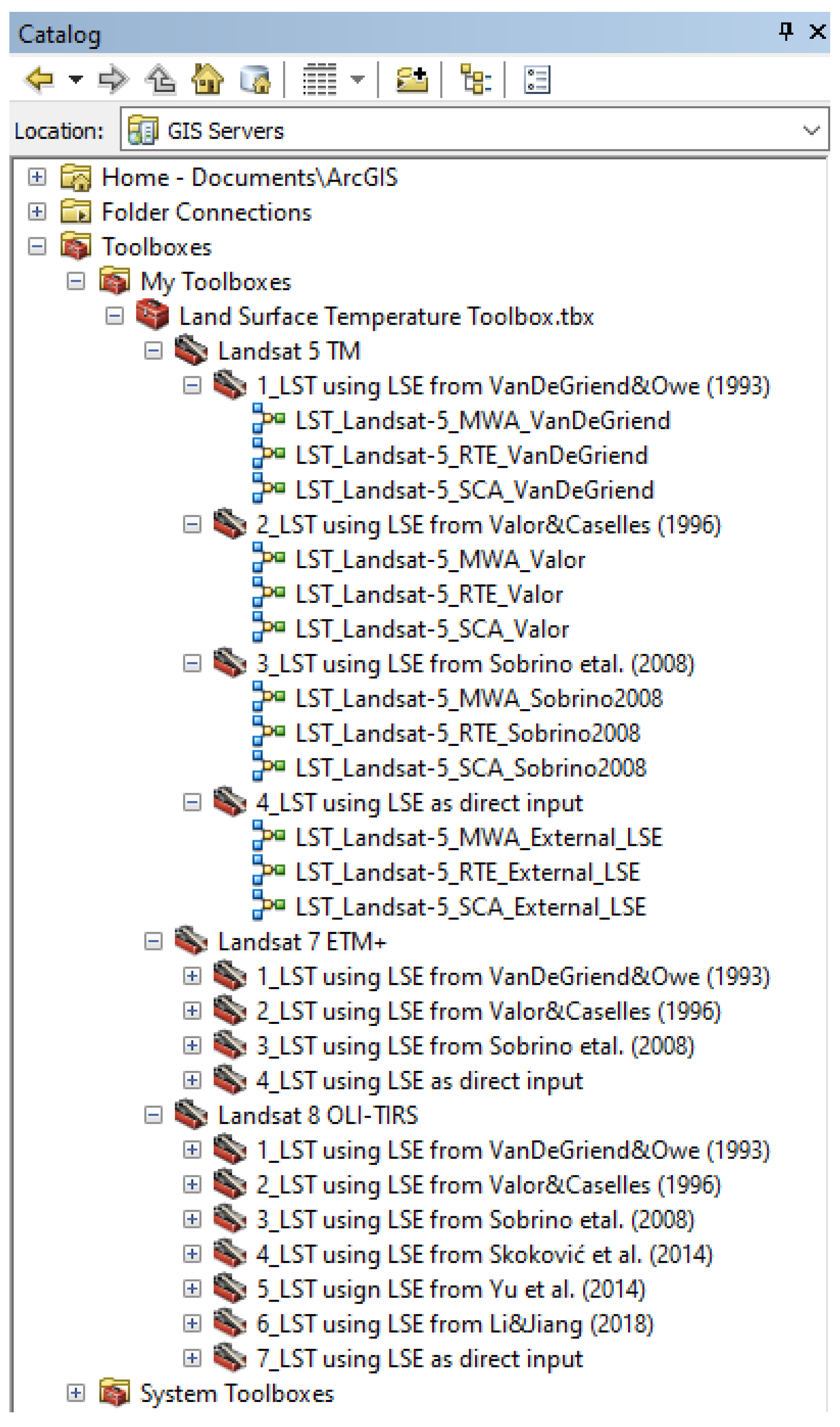
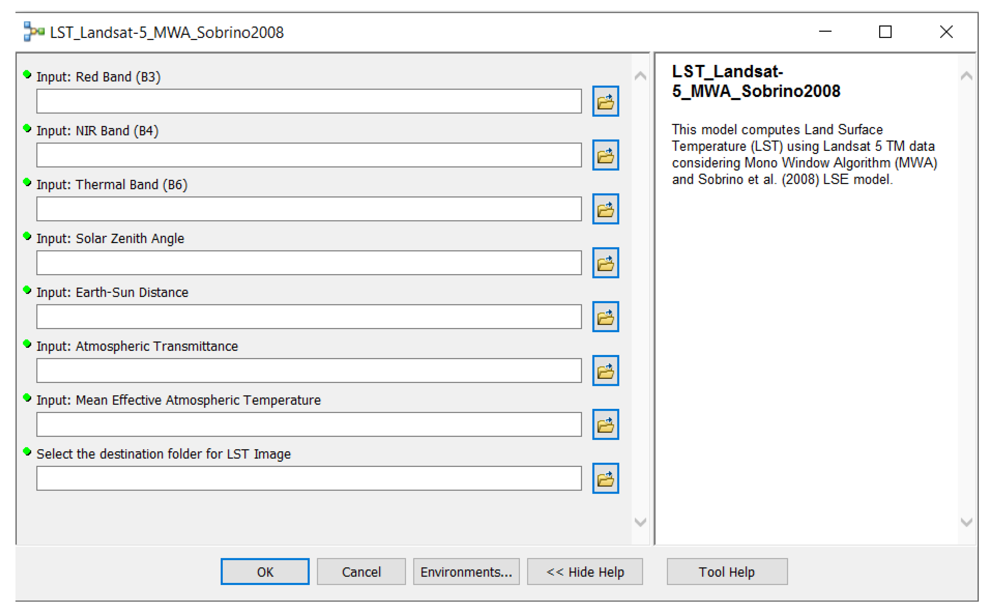
63]. In this work, a total of forty-five Landsat scenes, fifteen images for each Landsat mission, acquired in the Spring-Summer-Autumn period over rural areas in the mid-latitude region in the Northern Hemisphere were obtained over five SURFRAD stations in the period of 2000–2019. Simultaneous in-situ LST data with satellite acquisitions, obtained from the correspondent SURFRAD station, were utilized for accuracy analyses. For the aim of the work, we developed an enhanced toolbox for automated LST retrieval from Landsat data by RTE, SCA, MWA, and SWA algorithms using different LSE models (Supplementary Materials). This toolbox is a first step to fill the gaps in the availability of different LST retrieval methods/LSE models in packaged Remote Sensing (RS) or Geographic Information System (GIS) software.

2. Data Set

2.1. Landsat Imagery

Landsat series of satellites have provided space-based moderate-resolution remote sensing data continuously for more than four decades. From 23 July 1972, in total, eight series of Landsat satellites were launched for Earth Observation (EO) purposes. Landsat 6 was the only satellite that failed to achieve orbit. The rest of the satellites have provided a unique resource for global change research and applications in agriculture, cartography, geology, forestry, regional planning, surveillance, and education over the last four decades. In this study, fifteen images for each Landsat series of 5, 7, and 8 were utilized for LST retrieval. The acquisition years of Landsat data range from 2000 to 2019, and only clear-sky images were considered. The selected dates ensure the presence of the in-situ data and the same number of images for the three Landsat missions. Landsat data can be downloaded through the USGS ’Earth Explorer’ website free of charge.
Landsat 5 TM and Landsat 7 ETM+ have six reflective bands (visible, near-infrared, and short-wavelength infrared, 30-m spatial resolution) and one band in the TIR region (Band 6). The thermal band has a native spatial resolution of 120-m and 60-m for TM and ETM+, respectively, but it is delivered by USGS at 30-m after cubic convolution resampling. The Landsat 8 OLI sensor has nine reflective bands with 30-m spatial resolution, and Landsat 8 TIRS sensor has two bands in the TIR region (Band 10 and Band 11). These thermal bands have a 100-m native spatial resolution but resampled and published at 30 m by USGS.
Appendix A reports the information of Landsat data utilized in the study (forty-five images from 2000 to 2019), as well as meteorological data (near-surface temperature and relative humidity) and NDVI value information corresponding to the acquisition times of Landsat data.

2.2. SURFRAD Data and Validation Sites

SURFRAD network was established by NOAA Office in 1993 in order to support climate-related researches over the US. SURFRAD stations have been measuring accurate, continuous, and long-term in-situ surface radiation budget [63]. The system became operational in 1995 with four stations, and, currently, eight SURFRAD stations are operating in different climatological regions of the US. Upwelling and downwelling components of solar and infrared radiation are the primary measurements. Besides, ancillary observations include direct and diffuse solar radiation, ultraviolet-B radiation, and meteorological parameters. Since SURFRAD stations provide unique in-situ LST information over rural sites, many researchers have used these data to validate satellite-based LST retrievals [15,46,52,53,56,64,65,66,67]. In this study, five SURFRAD stations were considered as ground-based stations, and Table 1 reports information regarding the SURFRAD experimental sites. We also analyzed the LST retrieval at the SURFRAD station of Table Mountain, Boulder, Colorado (TBL). However, the LST differences between the satellite and the ground were high due to its elevation and the heterogeneity of the land cover as also assessed in other studies [15,59,68,69]. Thus, TBL station was not considered in the analyses. SXF (Sioux Falls, South Dakota) and SGP (ARM Southern Great Plains Facility, Oklahoma) station data were not processed in this study.
The native spatial resolution of the Landsat thermal channels spans from 60 to 120 m, even if pixels are resampled at 30 m by USGS. The SURFRAD pyrgeometer used to measure the upwelling radiation is deployed at a 10-m high tower, producing an effective diameter of the field-of-view of about 40 m at the surface, i.e., roughly of the same order of the Landsat pixel size. Therefore, the Landsat pixel covering the SURFRAD instrument was selected for the comparison test.

3. LST Retrieval Methods

As previously pointed out, the following four LST retrieval methods will be considered: Mono Window Algorithm (MWA) [43], Single Channel Algorithm (SCA) [44], Radiative Transfer Equation (RTE) method and Split Window Algorithm (SWA) [45,46]. While the first three methods can be applied to Landsat 5 TM, 7 ETM+ and 8 OLI/TIRS data, the SWA is applicable only to Landsat 8 OLI/TIRS data, since it requires at least two TIR bands. The essential differences between these methods are in the mathematical formulation and the input parameters [70]. In addition to the emissivity and the atmospheric transmissivity common to all methods, MWA needs near-surface air temperature for the effective mean atmospheric temperature computation unlike other methods. Conversely, RTE and SCA require the upwelling and downwelling atmospheric radiances for LST retrieval. The sensitivity of the input parameters on LST retrieval methods is reported in Appendix D.

3.1. Mono Window Algorithm

Mono Window Algorithm (MWA) was developed by Qin et al. [43] for Landsat TM data. The method requires three main parameters, i.e., emissivity, atmospheric transmittance, and effective mean atmospheric temperature. LST values from MWA can be estimated as:
T s = { a · ( 1 C D ) + [ b · ( 1 C D ) + C + D ] · T D · T a } ÷ C a = 67.355351 ,   b = 0.458606 ,   C = ε × τ ,   D = ( 1 τ ) [ 1 + ( 1 ε ) × τ ]
where Ts is the LST in Kelvin, T is the at-sensor brightness temperature in Kelvin, Ta is the effective mean atmospheric temperature in Kelvin, τ is the atmospheric transmittance, ε represents LSE, a and b are the algorithm constants, C and D are the algorithm parameters calculated using LSE and transmittance. A detailed description of the computations of the T, Ta and τ parameters adopted in this work, are reported in Appendix B. The different LSE models tested in this work will be described in Section 4.

3.2. Single-Channel Algorithm

Jiménez-Muñoz et al. [44] introduced a revision of the Single-Channel Algorithm (SCA) to retrieve LST from Landsat TIR data. Considering SCA, LST (Ts) can be computed using the following general equation:
T s = γ [ 1 ε ( ψ 1 L sen + ψ 2 ) + ψ 3 ] + δ
where ε is the LSE, Lsen is the at-sensor radiance of thermal band, ψ1, ψ2, and ψ3 are atmospheric functions, and γ, δ are two parameters given by:
γ T 2 b γ L sen
δ T T 2 b γ
where bγ = c2i with c2 = 14,387.7 µm∙K and λi is the effective band wavelength for band i, which is defined as:
λ i = λ 1 , i λ 2 , i λ f i ( λ ) d λ λ 1 , i λ 2 , i f i ( λ ) d λ
where fi(λ) is the spectral response function for the corresponding band. λ1, i and λ2, i are the lower and upper boundary of fi(λ), respectively. The value of bγ is equal to 1256 K and 1277 K for Band 6 of Landsat 5 and Landsat 7, respectively; for Band 10 and Band 11 of Landsat 8, it is equal to 1320 K and 1199 K, respectively.
Atmospheric functions ψ1, ψ2, and ψ3 are defined as:
ψ 1 = 1 τ   ;   ψ 2 = L λ L λ τ ; ψ 3 = L λ
where L λ (W∙m−2∙sr−1∙μm−1) is upwelling or atmospheric path radiance, L λ (W∙m−2∙sr−1∙μm−1) is downwelling or sky radiance. In this study, the atmospheric parameters τ, L λ and L λ used for the ψ1, ψ2, and ψ3 computation are reported in Appendix B.

3.3. Radiative Transfer Equation Method

A straightforward method to retrieve LST from a single TIR band is the inversion of the radiative transfer equation (RTE) according to the following expressions:
L λ sen = [ ε B λ ( T s ) + ( 1 ε ) L λ ] τ + L λ
where L λ sen (W∙m−2∙sr−1∙μm−1) is at-sensor registered radiance of the related thermal band, Bλ (W∙m−2∙sr−1∙μm−1) is the blackbody radiance. Blackbody radiance (Bλ) at a temperature of Ts can be obtained by inverting the Equation (7):
B λ ( T s ) = L λ sen L λ τ ( 1 ε ) L λ τ ε
and, finally, Ts can be obtained by inverting Planck’s law as:
T s = K 2 ln ( K 1 L λ sen L λ τ ( 1 ε ) L λ τ ε + 1 )
where K1 and K2 are calibration constants for Landsat data reported in Appendix B.

3.4. Split-Window Algorithm

In previous studies, various Split Window Algorithms (SWAs) have been introduced for different sensors [4,71,72,73,74] and detailed information of SWAs is reported in [7]. Among the different SWAs in the literature, in this study we considered SWA developed by Mao et al. [45] with coefficients re-parameterized by Yu et al. [46], corresponding to the Landsat 8 TIRS’ spectral response curve. The USGS recommended not to use Band 11 of Landsat 8 for LST retrieval due to the large calibration uncertainty [75]. However, some researchers claimed that they obtained satisfactory results via SWA [46,76]. Thus, we also analyze and present SWA results in this study. According to SWA, LST (Ts) can be calculated using the following equations:
T s = T 10 + B 1 ( T 10 T 11 ) + B 0
B 0 = C 11 ( 1 A 10 C 10 ) L 10 C 10 ( 1 A 11 C 11 ) L 11 C 11 A 10 C 10 A 11
B 1 = C 10 C 11 A 10 C 10 A 11
A 10 = ε 10 τ 10
A 11 = ε 11 τ 11
C 10 = ( 1 τ 10 ) ( 1 + ( 1 ε 10 ) τ 10 )
C 11 = ( 1 τ 11 ) ( 1 + ( 1 ε 11 ) τ 11 )
where ε 10 and ε 11 represent LSE for Band 10 and 11, respectively, τ 10 and τ 11 the atmospheric transmittance for Band 10 and 11, respectively, calculated as reported in Appendix B. L10 and L11 can be computed from Table 2 within a specific brightness temperature range for Band 10 (T10) and Band 11 (T11), respectively. In Table 2, “a” is the slope and B(K) is the intercept of linear regression. For example, if the brightness temperature of B10 ranges between 20 and 50 °C, L10 can be calculated by 0.4464 * T10 − 66.61.

4. Land Surface Emissivity (LSE) Models

Surface emissivity stands for the surface ability that transforms heat energy into radiant energy [36]. LSE (ε) is one of the key parameters to retrieve accurate LST from remotely sensed imagery. Semi-Empirical Methods (SEMs), Physically-Based Methods (PBMs), and multi-channel Temperature/Emissivity Separation (TES) methods are three distinctive categories for LSE retrieval from space [7]. PBMs and multi-channel TES methods are not operational for Landsat data to obtain LSE due to the limitations presented in many studies, such as the requirement of more than two TIR bands or nighttime images [7,46,76,77,78,79]. SEMs contain the Classification Based Emissivity Method (CBEM) [74,80] and the NDVI Based Emissivity Method (NBEM) [81,82], which are suitable for LSE estimation from Landsat data. The CBEM generates an LSE image from a classified image by applying an emissivity value for each class. However, CBEM is not practical since it requires a good knowledge of the study area and emissivity measurements on the surfaces representative of the different classes [70]. NDVI-based methods are operative and the most commonly utilized LSE retrieval methods since they are easy to apply and presenting satisfying results [36,58,83]. Li et al. [7] presented a detailed study showing the advantages, disadvantages, and limitations of different LSE models for LST retrieval from satellite data. Considering the study of Li et al. [7] and other researches, a state-of-the-art table showing different LSE categories and models, as well as the correspondent satellite data used is reported (Table 3).
As presented in Table 3, there are six NDVI-based models introduced for Landsat data, specifically three for Landsat TM and three for Landsat 8 OLI/TIRS. Therefore, we investigated the effect of these six LSE models on the accuracy of LST retrieval methods. Details about LSE models are presented in the following sub-sections. The sensitivity of the LSE on LST retrieval methods is reported in Appendix D.

4.1. LSE Model of Van de Griend and Owe

This model was applied to LST retrieval methods of all Landsat series (Landsat 5 TM, 7 ETM+, and 8 OLI/TIRS). Van de Griend and Owe [83] proposed a logarithmic approach for an LSE retrieval model based on NDVI ranging from 0.157 to 0.727. NDVI is obtained using the Near-Infrared (NIR) and Red (R) bands—the calculation steps of NDVI for Landsat 5, 7, and 8, are presented in Appendix C. The proposed model is given by:
ε = 1.0094 + 0.047 ln ( NDVI )

4.2. LSE Model of Valor and Caselles

This model was applied to LST retrieval methods of all Landsat series (Landsat 5 TM, 7 ETM+, and 8 OLI/TIRS). Valor and Caselles [82] proposed a theoretical model that relates the emissivity to the NDVI of a given surface by:
ε = ε v P v + ε s ( 1 P v ) + 4 d ε P v ( 1 P v )
ε v and ε s represent the emissivity of vegetation and soil, respectively. d ε is a term accounting for the cavity effect, which depends on the surface geometry. Pv (also referred to as fractional vegetation cover, FVC) is the proportion of vegetation calculated as [103]:
P v =   [ NDVI     NDVI min NDVI max     NDVI min ] 2
where NDVImax = 0.5 and NDVImin = 0.2 in a global situation [70]. As Valor and Caselles [82] suggested, ε v and ε s as 0.985 and 0.960, respectively, for unknown emissivity and vegetation structures, we also regarded these emissivity values in the calculation. Besides, they calculated the mean value for d ε term as 0.015, and we utilized this value in LSE retrieval with this model. The final version of the LSE model can be given by:
ε = 0.985 P v + 0.960 ( 1 P v ) + 0.06 P v ( 1 P v )

4.3. NDVI Threshold (NDVITHM)-Based LSE Models

Sobrino et al. [58], Skoković et al. [60], Yu et al. [46], and Li and Jiang [76] estimated LSE from NDVI threshold (NDVITHM) values considering three different cases as presented in Equation (21). In the first case (NDVI < 0.2), the pixel is considered as bare soil, and the emissivity is obtained from the reflectance values in the red region. In the second case (0.2 ≤ NDVI ≤ 0.5), the pixel is composed of a mixture of bare soil and vegetation, and in the third case (NDVI > 0.5), the pixels with NDVI values higher than 0.5 are considered as fully vegetated areas.
ε = { a i ρ R + b i NDVI < 0.2 ε v + ε s ( 1 P v ) + d ε , d ε = ( 1 ε s ) ( 1 P v ) F ε V 0.2 NDVI 0.5 ε V + d ε NDVI > 0.5
In Equation (21), ρ R is the reflectance value of the red band, a i and b i are estimated from an empirical relationship between the red band reflectance and Moderate Resolution Imaging Spectroradiometer (MODIS) emissivity library. ε v and ε s are the soil and vegetation emissivity, respectively. d ε is the cavity effect due to surface roughness as in the previous model ( d ε = 0 for flat surfaces). F is a geometrical shape factor assumed as the mean value of 0.55 [70]. Table 4 presents the expressions of NDVITHM for all models mentioned above.
In Li and Jiang’s LSE model, ρ j is the apparent reflectance in the OLI band j and a 1 i a 7 i are coefficients obtained from [76]. The LSE models of Band 11 were just utilized in the SWA method. It is important to point out again that the USGS announced caution in the use of Band 11 of Landsat 8 due to the calibration uncertainties [75]. However, some researchers published satisfactory results by using SWA [46,76].

5. LST Computation Using Ground-Based SURFRAD Data

As stated in Section 2.2, image-based LST results were validated using the data of five ground-based SURFRAD stations. Since these stations do not provide LST measurements directly, LST is calculated from the upwelling and downwelling longwave radiation measurements using the following Equation (22) with regard to the Stefan–Boltzmann law:
LST = [ F λ ( 1 ε b ) · F λ ε b · σ ] 1 / 4
where F λ and F λ represent upwelling and dowelling thermal infrared (3–50 μm) irradiance in W/m2, respectively, measured during satellite passages. σ is the Stefan–Boltzmann constant (5.670367 × 10⁻⁸ W∙m−2∙K−4), and ε b represents the broadband longwave surface emissivity, which is not measured by the station instruments. In previous studies on SURFRAD stations [53,56,65], the broadband emissivity was computed as reported in [104,105] by regression from narrowband emissivity of MODIS thermal bands, which are available through the MODIS monthly emissivity data set. The results in [104,105] proved that the longwave broadband emissivity for the SURFRAD sites could be considered 0.97, as also assumed in [64] and [53].
Therefore, in this study, the broadband emissivity was assumed 0.97. This assumption impacts only the SURFRAD LST estimation, not the satellite-derived estimation. Heidinger et al. [66] investigated the impact of changing the assumed broadband emissivity from 0.97 to 0.98 on the SURFRAD LST observation. The results indicated that a 0.01 error in broadband emissivity produces a SURFRAD LST error that rarely exceeds 0.25 K. In addition, Wang and Liang [105] proved that the sensitivity of the SURFRAD LST to broadband emissivity ranged from 0.1K/0.01 to 0.35K/0.01, which means the accuracy of LST varies between 0.1 K to 0.4 K when the broadband emissivity error is about ±0.01. While this error is not negligible, it does not appear to be a dominant source of uncertainty in the SURFRAD-based performance metrics considering the magnitude of the other uncertainties [66].
Satellite-based LST and SURFRAD-based LST were compared using statistical criteria, namely, the Root Mean Square Error (RMSE). RMSE, in Equation (23), is a widely used statistical metric evaluating the efficiency of the models.
RMSE = [ T SAT     T SURF ] 2 n
where T SAT and T SURF are the satellite-based LST and SURFRAD-based LST, respectively, and n represents the pixel count.

6. Results

In order to compare the results of LST retrieval methods, fifteen images of each Landsat mission (Landsat 5, 7, and 8), a total of forty-five images, were utilized in this study. MWA, RTE, and SCA were performed for all satellite data, whilst SWA was only utilized with Landsat 8 data due to the requirement of two TIR bands. The values of the atmospheric and model parameters used in LST retrieval methods for the 45 images are reported in Appendix E. Furthermore, the effects of different LSE models on the accuracy of the LST retrieval methods were investigated.

6.1. Results of LST Algorithms and LSE Models Derived from Landsat 5 TM

In Table 5, the accuracy of LST retrieval methods for Landsat 5 TM data is presented based on the different LSE models. Considering the LSE models, Sobrino et al.’s model provided the best results for all three LST retrieval methods. Valor and Caselles’ model was the second LSE model presenting satisfying results for LST estimation, whilst Van De Griend and Owe’s LSE model provided very high RMSE. The SURFRAD test assessed whether the RTE method was a bit better than MWA and SCA, with a lower RMSE value of 2.35 K.

6.2. Results of LST Algorithms and LSE Models Derived from Landsat 7 ETM+

In Table 6, validation results for Landsat 7 ETM+ data are reported. Again, Sobrino et al.’s model provided the best results whilst both Valor & Caselles’ model and Van De Griend & Owe’s LSE models presented much higher RMSE values. Although all LST retrieval methods with Sobrino et al.’s LSE model presented good results when using Landsat 7 ETM+ data, the results revealed that MWA provided slightly better results than RTE and SCA (RMSE value equals to 2.24 K).

6.3. Results of LST Algorithms and LSE Models Derived from Landsat 8 OLI/TIRS Data

In Table 7, the accuracy of LST retrieval methods for Landsat 8 OLI/TIRS data is assessed considering six LSE models. Again, Sobrino et al.’s model presented the best results as for Landsat 5 TM and 7 ETM+. The three LSE models Skoković et al., Yu et al., and Li & Jiang, specifically proposed in the literature for Landsat 8 data, also showed good results for all LST retrieval methods (the highest RMSE is 3.22 K). The LSE models of Valor & Caselles and Van De Griend & Owe presented the worst RMSE values again. This test suggests that MWA with Sobrino et al.’s LSE model provides better results than RTE and SCA, with a lower RMSE value (2.52 K). Considering the SWA method, requiring two emissivity images corresponding to the two TIR bands of Landsat 8 (Band 10 and 11), the three LSE models (Skoković et al., Yu et al., and Li & Jiang) provided satisfactory results. However, Skoković et al.’s LSE model demonstrated a slightly better RMSE value.

6.4. Comparison of LST Retrieval Algorithms Considering All Landsat Missions

In Section 6.1, Section 6.2 and Section 6.3, LST results were analyzed by dividing the sensor types of Landsat missions. In this section, the accuracies of the LST retrieval algorithms with respect to the ground-based LST data were evaluated considering the best LSE Model (Sobrino et al.’s) and all Landsat missions. This comparison can be significant for users who will conduct time-series analyses of LST over rural areas using the data of all Landsat missions. Since SWA was only used with Landsat 8 data, but it is not the best retrieval method, it was not considered in this section for the comparison purposes. In Figure 1a–c, MWA-based, RTE-based, and SCA-based LST results derived from Landsat 5, 7, and 8 data were compared with SURFRAD LST, respectively. The RMSE was 2.39 K for MWA, 2.57 K for RTE, and 2.73 K for SCA. The average biases (ground LST-satellite LST) for MWA, RTE, and SCA are −0.72 K, −1.63 K, and −1.81 K, respectively. Moreover, the error standard deviations (STD) are 2.28 K, 1.98 K, and 2.05 K for MWA, RTE, and SCA, respectively. Even though MWA has a slightly greater error STD, overall, the RMSE for RTE and SCA is higher due to the greater biases. This in-situ test over different rural areas showed that MWA, RTE, and SCA can provide good results with Sobrino et al.’s LSE model, and MWA presented slightly better performance. Figure 1 and biases show that although all methods tend to overestimate LST slightly, the MWA overestimation is lower. The different results, especially the bias, can be ascribed to the accuracy of the input parameters: as reported previously, RTA and SCA have the same input parameters, whilst MWA uses Ta instead of L λ and L λ . We must also consider the different formulation of the methods: since SCA is derived from a mathematical approximation of RTE [41], it is expected they provide similar results.

6.5. Analysis of Spatio-Temporal and Seasonal LST Variations Between LST Retrieval Methods

As stated in previous sections, Sobrino et al.’s LSE model provided the best performance on all LST retrieval methods. In this section, we focus on investigating the spatio-temporal and seasonal relationship between the LST retrieval methods using the Sobrino et al.’s LSE model. This analysis does not represent an evaluation of the best LST retrieval method, which was assessed in previous sections by a test with SURFRAD data, but it suggests us if there is similarity or not between the three methods (MWA, RTE, and SCA) with the same LSE model under changing emissivity values due to seasonal variations. In this analysis, we consider the LST retrieval methods in a rural area of 6 km × 6 km (40,000 pixels) centered on the SURFRAD station of each Landsat image. Therefore, a total of 45 × 3 LST sub-images (45 Landsat images × 3 LST methods) were investigated. Figure 2 shows an example of Landsat 8 LST image over the 6 × 6 km2 rural area, acquired on 27 April 2018 and covering the BND station, for the three methods used in this analysis.
To analyze the spatio-temporal and seasonal LST variations among the LST retrieval methods, the 45 Landsat images were categorized into three seasons: spring (18 images), summer (13), and autumn (14), and Root Mean Square (RMS) differences were calculated for each image. Winter images were not available due to cloudy conditions (see Table A1). This is not an accuracy test as the one performed by the SURFRAD LST ground measurements, but it is an image-based analysis to highlight the differences among the three retrieval methods. Therefore, the RMS difference is used instead of the RMSE. In the 6 × 6 km2 selected areas, the minimum LST values from satellite data for spring, summer, and autumn are 280.29 K, 281.70 K, and 284.67 K, respectively; the maximum are 321.88 K, 330.67 K, and 317.95 K, respectively. Figure 3 shows the box-plot graph presenting the seasonal RMS differences between the LST retrieval methods. The box-plot is used to display distributional characteristics of data [106]. The box-plot information, reported in Figure 3 by numbers, is the minimum (1) (the lowest data point excluding any outliers), first quartile (2), median (3), third quartile (4) and maximum (5) (the largest data point excluding any outliers). The cross “x” in the boxes refers to the mean value of the data set, and the points outside the minimum, and maximum values are assumed as outliers. Concerning Figure 3, blue box-plots represent the RMS differences between MWA and RTE-based LST values across the seasons. Red and orange box-plots refer to the RMS differences between RTE and SCA-based LST values, and SCA and MWA-based LST values, respectively.
Figure 3 highlights that RTE and SCA have a high level of agreement with each other regardless of the season. MWA is slightly different from RTE and SCA, and in the summer this difference is more evident due to the higher LST dynamics. Since SCA is derived based on RTE [41], and they have the same input parameters, their similarities can also be seen in Figure 3. MWA, on the other hand, uses Ta instead of L λ and L λ considered by RTE and SCA. Although the median values of all box-plots and seasons are close to zero (0.11–0.35 K for spring, 0.18–0.94 K for summer, and 0.12–0.43 K for autumn), MWA provides clearly different LST values than RTE and SCA in some summer images. In addition, the mean RMS differences (the cross “x” in boxes) (0.11–0.59 K for spring, 0.24–1.91 K for summer, and 0.12–0.64 K for autumn) reveals the higher variations between MWA and the other two methods in summer. Besides, there are two evident outliers over the maximum value in the summer and autumn for MWA-RTE and SCA-MWA.

6.6. Automated LST Extraction Toolbox for Landsat Missions

Different LST retrieval methods and LSE models are not available in packaged RS or GIS software. To overcome these difficulties, some researchers have developed plugins for different software such as ENVI [107], QGIS [108], ArcGIS [109], C++ [110], Python [111], Visual Basic [112] and ERDAS Imagine [113] to extract LST automatically. ERDAS Imagine and ArcGIS software present a visual programming interface which is of vital importance for users without specific knowledge of classical textual programming languages. The ModelBuilder is the visual programming language of ArcGIS software that enables connecting different steps of algorithms to automate the whole process.
GIS models and many remote sensing algorithms require a series of serial tasks called geo-processing workflows. Thanks to the geospatial models, all steps of an algorithm can be connected to each other to automate the whole process. Although ESRI’s ArcGIS is a commercial GIS software, many people and governmental institutions around the world utilize this software since it presents a substantial context for GIS users. Besides, it offers a powerful geospatial model builder (the ModelBuilder) that allows automation and documentation of an algorithm or method. Please see Appendix F for more information about the LST toolbox created based on this study (Supplementary Materials).

7. Discussion

As stated in Section 4, CBEM and NDVI-based LSE models are two appropriate models for Landsat data; CBEM can be used if emissivity measurements are obtained from in-situ campaigns, but it is not practical if the land cover information is not known accurately. Thus, we evaluated the impact of different NDVI-based LSE models, introduced in previous works, on LST retrieval methods over rural areas. It should be noted that the parameters and coefficients in NDVI-based LSE models were used as proposed in the original articles, and they can also be adapted to any study area with field campaigns. Valor and Caselles [82] stated that the error of their methodology ranges from 0.5% (due to the experimental limitations of the field methods) to 2% (considering the case in which there is no information about the study area). Van de Griend and Owe [83] did not conduct any sensitivity/error analysis but indicated that the correlation coefficient between NDVI and thermal emissivity was 0.941 at a 0.01 level of significance. One of the limitations of NDVI-based LSE models is its ineffectiveness in estimating LSE values for water and urban environments [114,115]. In this study, we just investigated the validation of daytime LST images. For nighttime LST evaluation, the LSE image can be estimated using CBEM derived from in-situ measurements or daytime NDVI-based LSE acquired on close dates. Overall, the proposed LST retrieval methods and LSE models can be implemented for regions other than the US, as well as for nighttime, non-rural, and winter data in clear sky conditions.
Considering the LST validation, error sources come from both satellite-based LST and ground-based LST. Satellite-based LST retrieval is still a challenging process due to the great variability of Earth surfaces and the necessary a priori knowledge about several parameters such as the atmosphere, the LSE, the meteorological conditions and the sensor specifications (spectral responses, signal to noise ratio, spectral resolution, spatial resolution, and viewing angle) [7,32,48,116,117,118]. Moreover, LST retrieval methods for satellite data are generally proposed considering different conditions and assumptions. Therefore, there is no universal method that always provides accurate LSTs from all satellite TIR data, and it is not easy to say which algorithm is superior to others [7]. The accuracy of the radiometric measurements and emissivity is the primary uncertainty for ground-based LST retrievals [119,120,121,122,123]. Sobrino and Skoković [119,122] presented an example of an error budget for The Global Change Unit (GCU) sites at the University of Valencia, and Table 8 indicates the impact of the parameter uncertainty ranges on ground-based LST.
It is interesting to discuss our results in comparison with those of other studies that utilized SURFRAD LST measurements and Landsat data for LST retrieval. Meng et al. [52] estimated LST from Landsat-8 data using the NOAA Joint Polar Satellite System (JPSS) Enterprise algorithm and a hybrid LSE model [82,124]. At the SURFRAD sites, the LST RMSE by the Enterprise algorithm was 3.22 K. Considering our analyses, SWA presented close results to the above analysis under three different LSE models ranging from 2.79 K to 3.02 K. Yu et al. [46] compared RTE, SWA, and SCA methods using Landsat 8 data with their LSE models reported in Section 4.3. They obtained satisfying RMSE values, i.e., 0.9 K, 1.39 K, and 1.03 K for RTE, SCA, and SWA, respectively. However, in this study, using Yu et al.’s LSE model, we obtained the RMSEs as 3.07 K, 3.18 K, and 3.02 K for RTE, SCA, and SWA, respectively. Zhang et al. [57] used Sobrino et al.’s LSE model and SCA method for LST retrieval from Landsat 8 data and compared four Landsat 8 LST images with SURFRAD measurements. Their results showed 1.11 K RMSE with reference to four LST images, whilst we computed 2.94 K RMSE using 15 LST images of Landsat 8 for the same LSE model and retrieval method. In addition to the previous study, Zhang et al. [53] also investigated the accuracy of SCA using Landsat 8 imagery and SURFRAD measurements using 40 Landsat 8 scenes acquired in different seasons and different years, and they obtained 1.96 K RMSE. Wang et al. [54] reported that Practical Single-Channel Algorithm (PSCA) and generalized SCA provided 1.77 K and 2.24 K RMSE, respectively, in line with our SCA results based on Landsat 8 and Sobrino et al.’s LSE model. Sekertekin [59] computed 3.12 K RMSE from 20 Landsat 8 images, close to the RTE-based Landsat 8 LST accuracy found in this test (2.73 K RMSE).
The limitations of this study and future investigations can be reported as follows: (1) Thermal bands have a native spatial resolution of 120 m, 60 m and 100 m for Landsat 5 TM, 7 ETM+, and 8 TIRS, respectively, but they are delivered by USGS at 30-m after cubic convolution resampling. Therefore, we also considered 30 m resampled TIR images which may lead to an error source when conducting pixel-scale validation. Different downscaling methods for TIR or LST data can be utilized as future work to examine the LST accuracy. (2) Although previous work proved that the accuracy of SURFRAD LST varies between 0.1 K to 0.4 K when the broadband emissivity error is about ±0.01, the use of fixed broadband emissivity (0.97) in this study may influence the ground-based LST calculation, but not dominantly. Broadband emissivity estimation models can be implemented in the future to show the optimal model for ground-based LST retrieval. (3) The LST toolbox, presented as a user facility in this study, does not include error analysis. Thus, users should carry out accuracy analysis after obtaining LST images. Besides, it can be improved and generated in an open-source environment as future work.

8. Conclusions

In this study, three LST retrieval algorithms (RTE, SCA, and MWA) were evaluated using Landsat 5 TM, 7 ETM+, and 8 OLI/TIRS data, and additionally, SWA were assessed for Landsat 8 OLI/TIRS data. Since LSE is one of the most important factors affecting the accuracy of LST retrieval methods, the effects of different NDVI-based LSE models on satellite-based LST accuracy were also investigated. Forty-five images acquired in the Spring-Summer-Autumn period over rural areas in the mid-latitude region in the Northern Hemisphere were obtained over five SURFRAD stations and simultaneous in-situ LST data were utilized for accuracy analyses. To get rid of step-by-step calculation for all LST methods and LSE models as well as for time consuming in processing of the images, an enhanced toolbox was generated for automated LST extraction. This toolbox can be utilized by all GIS users to obtain LST in an easy and practical way.
Three NDVI-based LSE models, namely, Sobrino et al.’s, Valor & Caselles’ and Van De Griend & Owe’s LSE model, were considered for Landsat 5 TM and 7 ETM+ data to investigate their effects on LST methods. In addition to these three LSE models, three more NDVI-based LSE models (Skoković et al.’s, Yu et al.’s, and Li and Jiang’s LSE models) were added to the analyses of Landsat 8 based LST methods. That is, the effects of six LSE models on the performance of LST methods from Landsat 8 data were investigated. To sum up, this study only considered NDVI-based LSE models for the evaluation of LST retrieval methods. Two different approaches were considered: 1) Sensor types of Landsat missions (Landsat 5, 7, and 8) were evaluated separately. 2) LST retrieval methods were compared with each other independently of sensor type, i.e., considering all Landsat missions together. In the toolbox, users can decide which LST method and LSE model they can utilize if they are dealing with the use of Landsat data. Furthermore, if they have their own LSE image, the toolbox makes it possible to use any external LSE image.
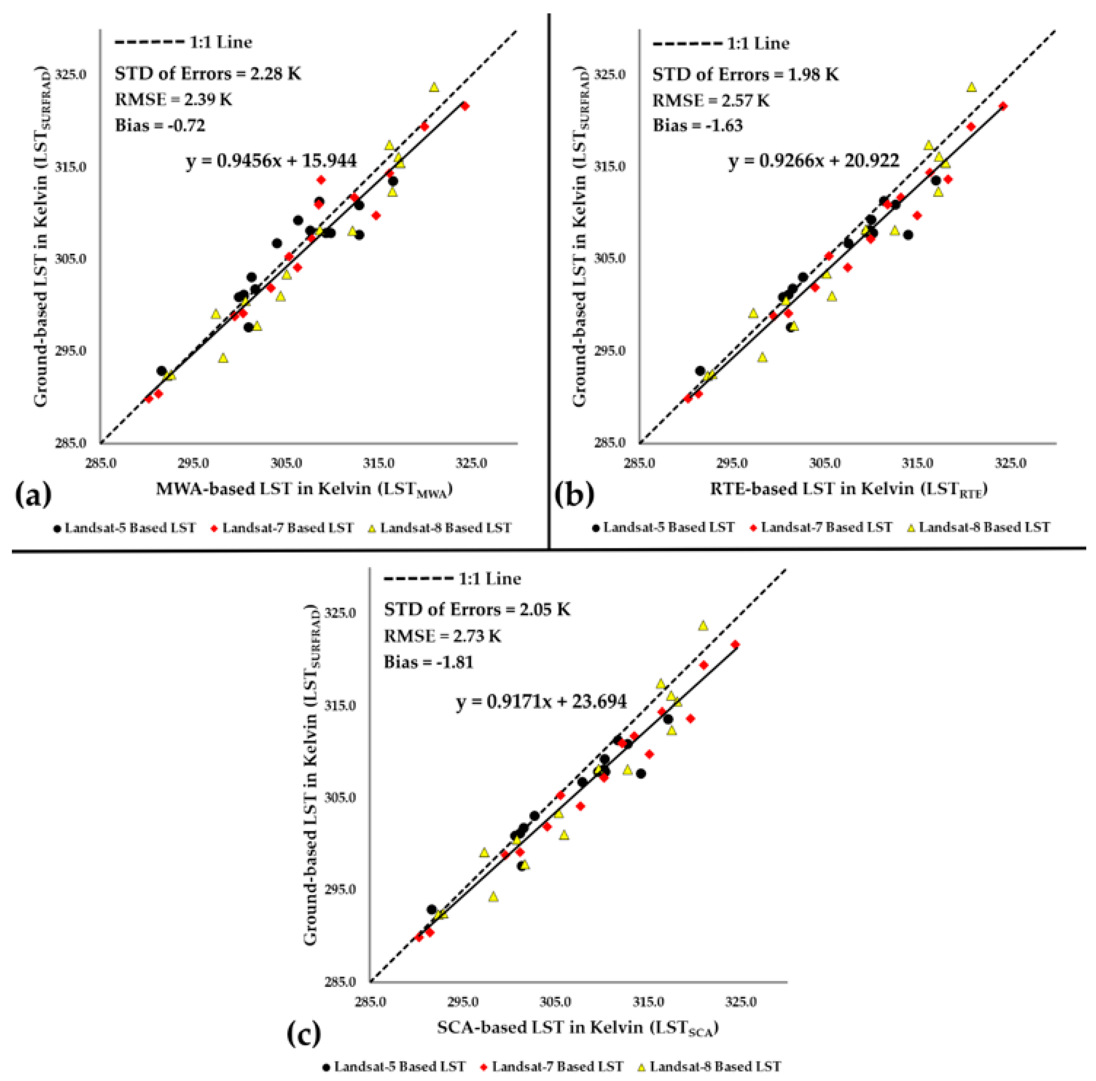
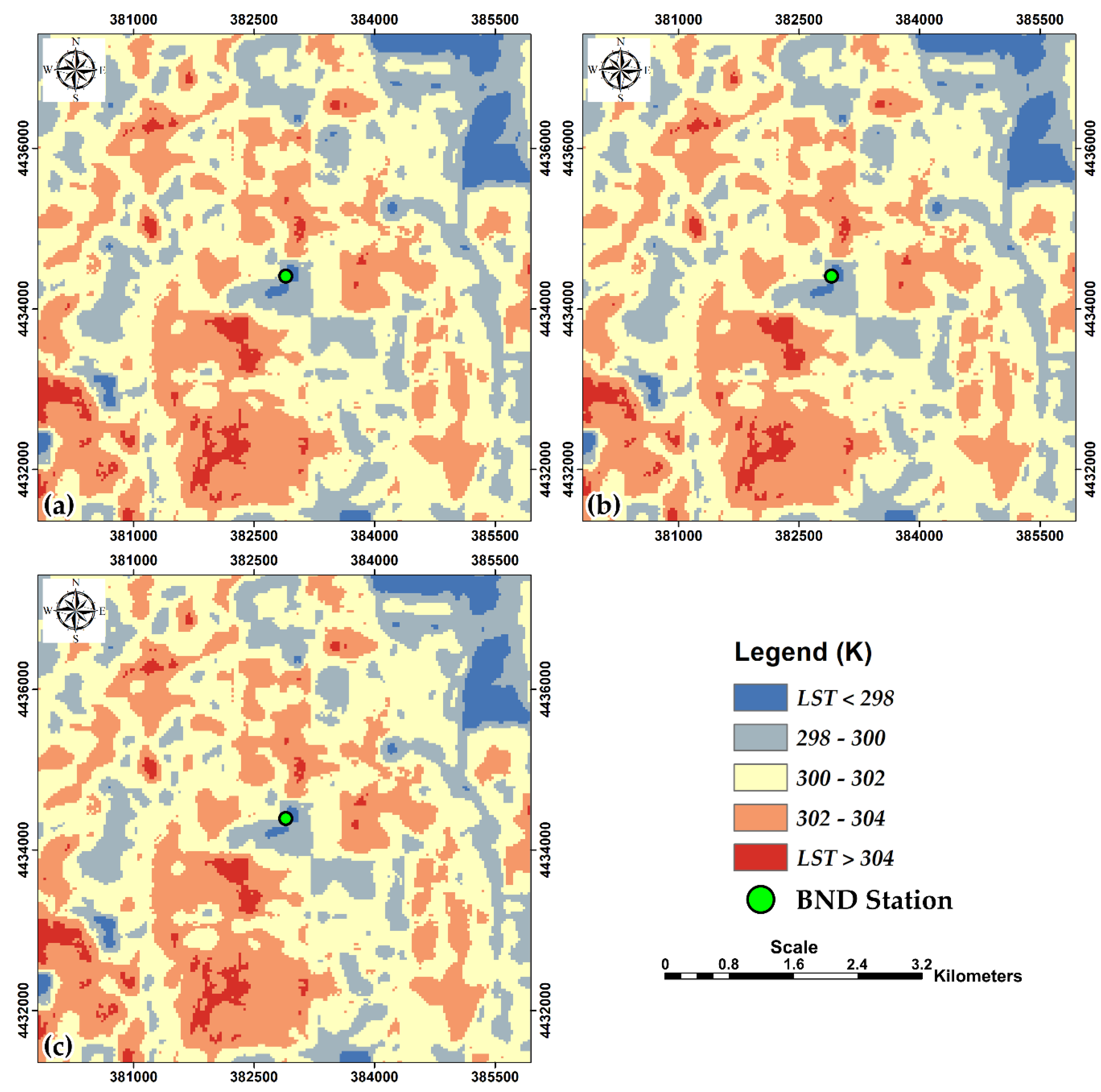
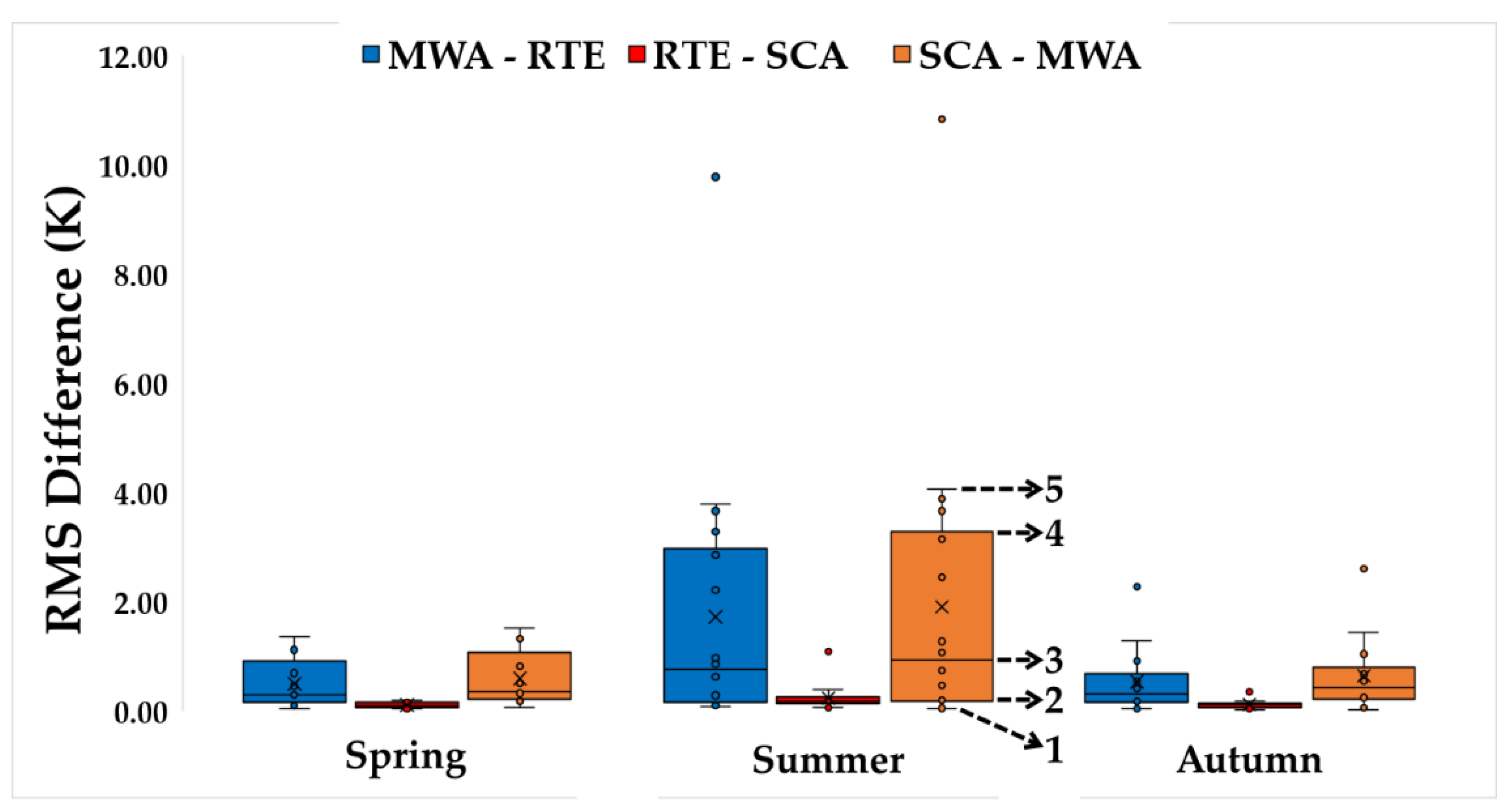
The obtained results showed that Sobrino et al.’s LSE model provided the best performance to extract LST for all Landsat missions and LST methods. Although all LST retrieval methods with Sobrino et al.’s LSE model presented satisfying and close results when using Landsat 5 TM data, RTE offered the best accuracy (2.35 K RMSE). The same would apply to Landsat 7 ETM+ data, even if MWA presented the best results (2.24 K RMSE). Again, Sobrino et al.’s LSE model provided higher accuracy for all LST retrieval methods from Landsat 8 data, with MWA as the best method (2.52 K RMSE). Considering all Landsat missions, MWA offered slightly better accuracy than RTE and SCA. Concerning the analyses above, it is hard to say which method is globally the best one, since the accuracy of the input parameters largely affects the performance of the methods. In addition, the spatio-temporal and seasonal comparison among LST retrieval methods revealed that RTE and SCA have a high level of agreement with each other regardless of the season. Instead, MWA presented different results than RTE and SCA, especially in summer.
The results indicated that LSE models have a great impact on the accuracy of satellite-based LST retrieval methods. This study also revealed that Sobrino et al.’s LSE model was the most appropriate model for all Landsat missions and LST retrieval methods over rural areas. Moreover, validation of LST retrieval methods with different LSE models over urban areas is a further challenge to be faced that deserves future investigations.

Supplementary Materials

The following are available online at https://0-www-mdpi-com.brum.beds.ac.uk/2072-4292/12/2/294/s1, code: Land surface Temperature Toolbox.

Author Contributions

Conceptualization—A.S.; methodology—A.S.; software—A.S.; validation—A.S.; writing—review and editing—A.S., S.B.; supervision—A.S., S.B. All authors have read and agreed to the published version of the manuscript.

Funding

This research received no external funding.

Acknowledgments

The authors thank USGS for providing Landsat 8 satellite imagery free of charge. In addition, the authors thank NOAA for providing in-situ LST measurements from SURFRAD stations publicly (ftp://aftp.cmdl.noaa.gov/data/radiation/surfrad/).

Conflicts of Interest

The authors declare no conflict of interest.

Appendix A

Table A1. Information about Landsat data used in the study (45 images from 2000 to 2019). The last column shows the SURFRAD station included within the satellite scene. SURFRAD codes can be found in: https://www.esrl.noaa.gov/gmd/grad/surfrad/sitepage.html or in Table A1.
SensorScene IDScene Acquisition Date and Time (UTC)Path-RowTo (°C)RH (%)NDVI ValueSURFRAD Station
LANDSAT 5 TMLT50230322007167PAC0116/06/2007–16:2923–3230.835.30.348BND
LT50220322008243GNC0130/08/2008–16:1522–3225.551.20.672
LT50230322010255PAC0112/09/2010–16:2623–3224.832.20.438
LT50400352006267PAC0124/09/2006–18:1540–3521.814.50.074DRA
LT50400352007142PAC0122/05/2007–18:1640–3520.79.60.075
LT50400352011281PAC0108/10/2011–18:1040–3516.831.30.088
LT50350262006136PAC0116/05/2006–17:3935–2623.826.50.228FPK
LT50350262008238PAC0125/08/2008–17:3235–2630.235.10.170
LT50360262011253PAC0110/09/2011–17:4336–2627.628.60.330
LT50230362002249LGS0106/09/2002–16:1123–3629.455.70.566GWN
LT50230362008218PAC0105/08/2008–16:2323–3630.660.20.578
LT50230362011242PAC0130/08/2011–16:2623–3631.233.60.552
LT50160322003267GNC0224/09/2003–15:3016–3215.957.50.698PSU
LT50160322008233GNC0120/08/2008–15:3916–3219.550.20.674
LT50160322009139GNC0119/05/2009–15:4016–3215.929.90.390
LANDSAT 7 ETM+LE70230322000284EDC0010/10/2000–16:2623–3213.035.50.515BND
LE70230322001254EDC0011/09/2001–16:2423–3224.140.00.535
LE70220322002186EDC0005/07/2002–16:1822–3230.751.40.097
LE70400352001165EDC0014/06/2001–18:1240–3523.312.8-0.025DRA
LE70400352001213EDC0001/08/2001–18:1140–3532.510.9-0.030
LE70400352002168EDC0017/06/2002–18:1040–3530.96.9-0.027
LE70350262000112EDC0021/04/2000–17:3935–2621.222.6-0.068FPK
LE70360262001217EDC0005/08/2001–17:4336–2628.232.8-0.068
LE70350262002181EDC0030/06/2002–17:3635–2623.332.5-0.073
LE70220362000117EDC0026/04/2000–16:2322–3618.943.40.300GWN
LE70230362000220EDC0007/08/2000–16:2823–3632.555.10.258
LE70220362001167EDC0016/06/2001–16:2122–3627.344.90.389
LE70160322000091EDC0031/03/2000–15:4516–327.837.7-0.029PSU
LE70160322002192EDC0011/07/2002–15:4116–3217.944.40.375
LE70160322002256EDC0013/09/2002–15:4016–3221.537.30.250
LANDSAT 8 OLI/TIRSLC80230322013247LGN0104/09/2013–16:3823–3223.957.20.621BND
LC80230322018101LGN0011/04/2018–16:3523–3212.857.20.421
LC80230322018117LGN0027/04/2018–16:3523–3215.232.40.622
LC80400352017121LGN0001/05/2017–18:2240–3523.514.00.110DRA
LC80400352018124LGN0004/05/2018–18:2140–3526.414.60.108
LC80400352018236LGN0024/08/2018–18:2240–3532.88.70.088
LC80350262017198LGN0017/07/2017–17:4835–2624.722.10.213FPK
LC80360262018160LGN0009/06/2018–17:5336–2627.551.20.370
LC80350262018249LGN0006/09/2018–17:4735–2621.838.40.232
LC80220362016281LGN0107/10/2016–16:3222–3627.544.00.410GWN
LC80220362017251LGN0008/09/2017–16:3222–3622.544.80.626
LC80220362018094LGN0004/04/2018–16:3122–368.643.10.397
LC80160322015124LGN0104/05/2015–15:5116–3224.324.10.365PSU
LC80160322016111LGN0120/04/2016–15:5116–3215.215.20.512
LC80160322019263LGN0020/09/2019–15:5316–3220.653.80.637

Appendix B

Appendix B.1. Brightness Temperature (T) Retrieval

The brightness temperature is the temperature of a blackbody that would emit an identical amount of radiation at a definite wavelength [125] and it can be calculated by inverting the Planck function. Considering satellite data, Thermal Infrared (TIR) pixel values are firstly converted into radiance from Digital Number (DN) values. Radiances for TIR band of Landsat 5 TM and 7 ETM+ are obtained using Equation (A1) [126]. Radiance values for Landsat 8 TIRs can be retrieved from Equation (A2) [127].
L λ = [ LMAX λ     LMIN λ QCALMAX QCALMIN ] × [ Q CAL QCALMIN ] + LMIN λ
where Lλ is Top of Atmosphere (TOA) spectral radiance (Watts/(m2∙srad∙μm)), QCAL is the quantized calibrated pixel value in DN, LMINλ (Watts/(m2∙srad∙μm)) is the spectral radiance scaled to QCALMIN, LMAXλ (Watts/(m2∙srad∙μm)) is the spectral radiance scaled to QCALMAX, QCALMIN is the minimum quantized calibrated pixel value in DN and QCALMAX is the maximum quantized calibrated pixel value in DN. LMINλ, LMAXλ, QCALMIN, and QCALMAX values are obtained from the metadata file of Landsat TM and ETM+ data. For Landsat 8:
L λ = M L · Q CAL + A L
where L λ is the TOA spectral radiance (Watts/(m2∙srad∙μm)),   M L is the band-specific multiplicative rescaling factor from the metadata, A L is the band-specific additive rescaling factor from the metadata, Q CAL is the quantized and calibrated standard product pixel values (DN). All of these variables can be retrieved from the metadata file of Landsat 8 data. After radiance conversion, brightness temperature image can be generated by Equation (A3) for all Landsat missions [126,127].
T   =   K 2 ln ( K 1 L λ + 1 )
where T refers to the effective at-satellite brightness temperature in Kelvin, K1 (Watts/(m2∙srad∙μm)) and K2 (Kelvin) are the calibration constants and Lλ is the spectral radiance. The values of the constants (K1 and K2) were presented in Table A2 since they change from sensor to sensor [126,127].
Table A2. Thermal band calibration constants for landsat satellites.
SATELLITEK1 (Watts/(m2∙srad∙μm))K2 (Kelvin)
Landsat 5 (Band6)607.761260.56
Landsat 7 (Band6)666.091282.71
Landsat 8 (Band10)774.891321.08
Landsat 8 (Band11)480.891201.14

Appendix B.2. Effective Mean Atmospheric Temperature (Ta) Retrieval

Table A3 reveals the practical equations to calculate effective mean atmospheric temperature (Ta) by means of near-surface temperature (To),essential for MWA [43]. In this work, mid-latitude summer region was considered for the calculation.
We used a mid-latitude summer region model for Ta in this work; however, the USA 1976 Standard atmosphere is also suitable for our test sites. Thus, we also investigated the difference in LST when using mid-latitude summer and USA 1976 Standard models with simulations, and we obtained almost 1 K difference in LST in the analyses.
Table A3. The effective mean atmospheric temperature estimation (Ta) using near-surface air temperature (To).
ModelMean Atmospheric Temperature (Ta) in Kelvin
USA 1976 StandardTa = 25.940 + 0.8805 × To
Tropical RegionTa = 17.977 + 0.9172 × To
Mid-latitude Summer RegionTa = 16.011 + 0.9262 × To
Mid-latitude Winter RegionTa = 19.270 + 0.9112 × To

Appendix B.3. Atmospheric Transmittance (τ), Upwelling Radiance ( L λ ), and Downwelling Radiance ( L λ ) Retrieval

National Aeronautics and Space Administration (NASA) provides an atmospheric correction tool, known as the Atmospheric Correction Parameter Calculator (ACPC) that calculates atmospheric transmissivity or transmittance, upwelling, and downwelling radiance. These atmospheric parameters were computed taking the National Centers for Environmental Prediction modeled atmospheric profiles as inputs to the MODTRAN radiative transfer code for a given site and date [128,129]. In this study, atmospheric transmittance, upwelling and downwelling radiance values were calculated using the ACPC for MWA, RTE, and SCA. Alternatively, a radiative transfer code can be used to estimate atmospheric transmittance, upwelling and downwelling radiance.
Considering Landsat 8 data, ACPC presents parameters just for Band 10. Thus, for SWA, atmospheric transmittance values of Band 10 and 11 (τ10 and τ11) were calculated using water vapor as presented in Table A4 [46].
In addition, we investigated how τ 10 and τ 11 vary when we use USA 1976 Standard atmosphere instead of mid-latitude summer model in SWA. The difference in τ 10 and τ 11 varies from −0.001 to 0.004 and −0.004 to 0.035, respectively, for the water vapor range of Table A4. As reported in Table A5 of Appendix D, a 1% uncertainty for transmissivity in SWA results in ±0.29 K variation in LST (Table A5).
Table A4. The relationship between atmospheric transmittance (τ10/11) and water vapor content (w).
ModelWater Vapor RangeEquation
Mid-latitude Summer Region0.2–3.0 g/cm2 τ 10 = 0.0164 w 2 0.04203 w + 0.9715
τ 11 = 0.01218 w 2 0.07735 w + 0.9603
Water vapor content (w) can be either accessed from meteorological stations or calculated from Relative Humidity (RH) and near-surface temperature (To) using the following equation [130]:
w i = 0.0981 × { 10 × 0.6108 × exp [ 17.27 × ( T o 273.15 ) 237.3 + ( T o 273.15 ) ] × RH } + 0.1697
where wi (g/cm2) is the water vapor content, To is the near-surface temperature in Kelvin, and RH (%) refers to the relative humidity.

Appendix C

In this appendix, the calculation steps of Normalized Difference Vegetation Index (NDVI) for Landsat 5, 7, and 8 are described.
For Landsat 5 and 7 data, firstly, radiance conversion is applied as in Equation (A1) and then reflectance value can be calculated by radiances using equation (A5) [126]. For Landsat 8 data, reflectance conversion can be applied to DN values directly as in Equation (A6) [127]. After obtaining reflectance values for Near-infrared (NIR) and Red (R) bands, NDVI can be retrieved using Equation (A7). In the following, the Equations (A5)–(A7) are reported.
ρ λ = π · L λ · d 2 ESUN λ · cos θ s
where ρ λ is unitless planetary reflectance, Lλ is the TOA spectral radiance (Watts/(m2∙srad∙μm)), d is Earth-Sun distance in astronomical units, ESUNλ is the mean solar exo-atmospheric spectral irradiances (Watts/(m2∙μm)) and θs is the solar zenith angle in degrees. ESUNλ values for each band of Landsat 5 and 7 can be obtained from the handbooks of the related mission [126]. θs and d values can be attained from the metadata file.
ρ λ =   M p · Q CAL + A p sin θ SE
where   M p is the band-specific multiplicative rescaling factor from the metadata, A p is the band-specific additive rescaling factor from the metadata, Q CAL is the quantized and calibrated standard product pixel values (DN) and θ SE is the local sun elevation angle from metadata file.
NDVI   =   ρ NIR     ρ R ρ NIR   +   ρ R
where ρ NIR is the reflectance band in the NIR region and ρ R refers to the reflectance band in the R region.

Appendix D

Since the input parameters used in the retrieval methods inevitably have errors, affecting the LST accuracy, some papers reported sensitivity analyses of the input parameters on LST methods [131,132,133]. In this appendix a sensitivity analysis of each retrieval method to a specific input parameter is carried out, with the other input parameters fixed (Table A5). The input parameters are: effective mean atmospheric temperature, LSE, atmospheric transmittance, upwelling radiance and downwelling radiance of the atmosphere.
We assumed the near surface air temperature to be 295 K, thus the effective mean atmospheric temperature is calculated as 289.24 K. The atmospheric transmittance was assumed to be 0.77 and upwelling and downwelling radiances were assumed as 1.74 W∙m−2∙sr−1∙μm−1 and 2.82 W∙m−2∙sr−1∙μm−1. We assumed the brightness temperature range from 285 K to 300 K, since the variation in the brightness temperature also affect the results. The LSE value was fixed as 0.97. Considering SWA, we observed the average difference between τ 10 and τ 11 as 0.05. Thus, we assumed τ 10 and τ 11 to be 0.82 and 0.77, respectively. A fixed value of 1.5 K for T10–T11 as in [131].
Table A5 dhows that LSE is the most important parameter influencing the results of MWA and SWA compared to the other inputs. The sensitivity of L λ to the results of RTE and SCA is higher than L λ .
Table A5. Sensitivity of the LST retrieval methods to the input parameters.
Input ParameterUncertaintyTb (K)Estimated impact on LST
MWARTESCASWA
LSE±0.01285±0.49 K±0.58 K±0.54 K±0.55 K
290±0.54 K±0.58 K±0.56 K±0.55 K
295±0.58 K±0.58 K±0.58 K±0.55 K
300±0.63 K±0.58 K±0.60 K±0.55 K
Atmospheric Transmittance±0.01285±0.09 K±0.97 K±0.89 K±0.29 K
290±0.01 K±0.97 K±0.93 K±0.29 K
295±0.08 K±0.97 K±0.96 K±0.29 K
300±0.16 K±0.97 K±0.99 K±0.29 K
Effective Mean Atmospheric Temperature±1 K285±0.32 KNot ApplicableNot ApplicableNot Applicable
290±0.32 KNot ApplicableNot ApplicableNot Applicable
295±0.32 KNot ApplicableNot ApplicableNot Applicable
300±0.32 KNot ApplicableNot ApplicableNot Applicable
L λ ±10%285Not Applicable±1.82 K±1.66 KNot Applicable
290Not Applicable±1.82 K±1.72 KNot Applicable
295Not Applicable±1.82 K±1.78 KNot Applicable
300Not Applicable±1.82 K±1.84 KNot Applicable
L λ ±10%285Not Applicable±0.07 K±0.06 KNot Applicable
290Not Applicable±0.07 K±0.06 KNot Applicable
295Not Applicable±0.07 K±0.07 KNot Applicable
300Not Applicable±0.07 K±0.07 KNot Applicable

Appendix E

Required atmospheric and model parameters were derived for each satellite image and presented in Table A6. In this table, atmospheric parameters include upwelling radiance ( L λ ), downwelling radiance ( L λ ), atmospheric transmittance (τ), and mean atmospheric temperature (Ta); model parameters include Earth-sun distance (d), solar zenith angle (θsz) for Landsat 5 and 7, and sun elevation angle (θse) for Landsat 8. L λ , L λ and τ were calculated using NASA’s ACPC (see Appendix B.3), and Ta was obtained from Table A3 for mid-latitude summer region. d and θse are obtained from metadata file of the Landsat data, and θsz is equal to 90o − θse. Earth-sun distance “d” is not necessary for Landsat 8 data to obtain spectral reflectance. Thus, this column in the table is empty for Landsat 8. In addition to Table A6, Table A7 presents transmittance values for Band 10 and Band 11 of Landsat 8 TIRS required for LST retrieval using SWA, and they were calculated from Table A4.
Table A6. Estimated atmospheric and model parameters used in this study for LST methods.
SensorScene Acquisition Date and Time (UTC)W/(m2*sr*µm)τTa (K)θsz (L5-7)/θse (L8) (°)d (Astronomical Unit)
L λ L λ
LANDSAT 5 TM16/06/2007–16:292.283.680.71297.5324.891.0159
30/08/2008–16:152.073.290.75292.6238.041.0095
12/09/2010–16:261.742.820.77291.9741.141.0064
24/09/2006–18:150.631.090.91289.1941.951.0031
22/05/2007–18:160.380.690.94288.1724.511.0123
08/10/2011–18:100.570.970.91284.5646.310.9991
16/05/2006–17:390.881.510.87291.0533.201.0112
25/08/2008–17:322.023.280.77296.9742.451.0106
10/09/2011–17:431.151.920.86294.5747.051.0070
06/09/2002–16:114.386.410.48296.2337.921.0079
05/08/2008–16:233.915.870.53297.3429.471.0143
30/08/2011–16:263.174.890.61297.9033.941.0097
24/09/2003–15:301.292.110.82283.7346.091.0032
20/08/2008–15:391.752.810.76287.0635.381.0117
19/05/2009–15:400.591.020.91283.7327.801.0118
LANDSAT 7 ETM+10/10/2000–16:260.480.810.93281.0450.450.9984
11/09/2001–16:241.732.80.78291.3241.071.0066
05/07/2002–16:183.315.130.6297.4426.841.0167
14/06/2001–18:120.510.910.93290.5824.101.0157
01/08/2001–18:110.951.630.88299.1028.811.0149
17/06/2002–18:100.691.220.92297.6224.351.0160
21/04/2000–17:390.771.320.88288.6440.001.0052
05/08/2001–17:431.62.640.8295.1236.621.0143
30/06/2002–17:360.821.410.89290.5830.751.0167
26/04/2000–16:231.282.10.82286.5129.201.0065
07/08/2000–16:284.877.090.41299.1028.931.0140
16/06/2001–16:211.813.160.76294.2923.801.0159
31/03/2000–15:450.420.710.93276.2341.370.9992
11/07/2002–15:410.81.350.89285.5827.491.0166
13/09/2002–15:401.312.160.83288.9241.681.0061
LANDSAT 8 OLI/TIRS04/09/2013–16:381.883.060.77291.1452.48 -
11/04/2018–16:350.881.490.87280.8653.35 -
27/04/2018–16:350.490.850.93283.0858.58 -
01/05/2017–18:220.50.90.93290.7762.45 -
04/05/2018–18:210.550.990.93293.4563.08 -
24/08/2018–18:220.641.150.93299.3858.18 -
17/07/2017–17:480.791.380.89291.8858.33 -
09/06/2018–17:532.223.610.73294.4760.62 -
06/09/2018–17:471.432.380.81289.1945.00 -
07/10/2016–16:322.173.510.74294.4746.10 -
08/09/2017–16:321.522.510.81289.8455.18 -
04/04/2018–16:310.350.60.94276.9754.73 -
04/05/2015–15:511.672.760.78291.5160.42 -
20/04/2016–15:510.450.770.94283.0856.60 -
20/09/2019–15:531.121.880.86288.0847.37 -
Table A7. Atmospheric transmittance values for Band 10 and Band 11 of Landsat 8 TIRS data used in SWA.
SensorScene Acquisition Date and Time (UTC) τ 10 τ 11
LANDSAT 8 OLI/TIRS04/09/2013–16:380.8390.777
11/04/2018–16:350.9130.871
27/04/2018–16:350.9330.898
01/05/2017–18:220.9420.912
04/05/2018–18:210.9360.904
24/08/2018–18:220.9410.910
17/07/2017–17:480.9240.886
09/06/2018–17:530.8200.755
06/09/2018–17:470.9010.855
07/10/2016–16:320.8470.787
08/09/2017–16:320.8830.832
04/04/2018–16:310.9380.906
04/05/2015–15:510.9210.882
20/04/2016–15:510.9510.925
20/09/2019–15:530.8760.822

Appendix F

In this study, a total of 49 individual models were generated in the ModelBuilder for automated LST retrieval using different LST retrieval algorithms and LSE models (Supplementary Materials). Apart from SWA, MWA, RTE, and SCA were modeled for Landsat 5 TM, Landsat 7 ETM+ and Landsat 8 OLI/TIRS data. Since SWA requires more than one thermal band, it can be only implemented for Landsat 8 TIRS data. Figure A1 illustrates the toolbox in ArcGIS catalog window showing the LST retrieval models for the related Landsat missions. The toolbox consists of three main parts with reference to the three Landsat missions, and each mission was categorized considering different LSE models for LST retrieval methods. Furthermore, if the users have their own LSE image generated by a model different from those studied here, they can also use this toolbox by selecting the external LSE model for each Landsat mission.
Figure A1. The interface of LST toolbox in the ArcGIS catalog window.
Remotesensing 12 00294 g0a1
In addition to Figure A1, the interface of the MWA method using Sobrino et al.’s LSE model and Landsat 5 TM data is presented in Figure A2 as an example. As shown in Figure A2, the users only select the required inputs and the destination folder for the LST image. Thus, this geospatial toolbox makes the processing of Landsat images much easier than step-by-step calculation. Researchers, who would like to use this toolbox, can get in touch with the authors without any hesitation.
Figure A2. The interface of the MWA method using the Landsat 5 TM data and Sobrino et al.’s LSE model.
Remotesensing 12 00294 g0a2

References

  1. Prakash, A. Thermal remote sensing: Concepts, issues and applications. In Proceedings of the International Archives of Photogrammetry and Remote Sensing, Amsterdam, The Netherlands, 16–22 July 2002; Volume 23, pp. 239–243. [Google Scholar]
  2. Kahle, A.B. Surface thermal properties. In Remote Sensing in Geology; Siegal, B.S., Gillespie, A.R., Eds.; John Wiley & Sons, Inc.: New York, NY, USA, 1980; pp. 257–273. ISBN 0471790524. [Google Scholar]
  3. Sabins, F.F. Remote Sensing: Principles and Interpretation, 3rd ed.; W. H. Freeman: New York, NY, USA, 1996; ISBN 0716724421. [Google Scholar]
  4. Wan, Z.; Dozier, J. A generalized split-window algorithm for retrieving land-surface temperature from space. IEEE Trans. Geosci. Remote Sens. 1996, 34, 892–905. [Google Scholar]
  5. Meng, X.; Cheng, J.; Liang, S. Estimating land surface temperature from Feng Yun-3C/MERSI data using a new land surface emissivity scheme. Remote Sens. 2017, 9, 1247. [Google Scholar] [CrossRef] [Green Version]
  6. Zhou, D.; Xiao, J.; Bonafoni, S.; Berger, C.; Deilami, K.; Zhou, Y.; Frolking, S.; Yao, R.; Qiao, Z.; Sobrino, J. Satellite remote sensing of surface urban heat islands: Progress, challenges, and perspectives. Remote Sens. 2018, 11, 48. [Google Scholar] [CrossRef] [Green Version]
  7. Li, Z.; Tang, B.-H.; Wu, H.; Ren, H.; Yan, G.; Wan, Z.; Trigo, I.F.; Sobrino, J.A. Satellite-derived land surface temperature: Current status and perspectives. Remote Sens. Environ. 2013, 131, 14–37. [Google Scholar] [CrossRef] [Green Version]
  8. Kerr, Y.H.; Lagouarde, J.P.; Nerry, F.; Ottlé, C. Land surface temperature retrieval techniques and applications. In Thermal Remote Sensing in Land Surface Processing; Quattrochi, D.A., Luvall, J.C., Eds.; CRC Press: Boca Raton, FL, USA, 2000; pp. 33–109. [Google Scholar]
  9. Karnieli, A.; Agam, N.; Pinker, R.T.; Anderson, M.; Imhoff, M.L.; Gutman, G.G.; Panov, N.; Goldberg, A. Use of NDVI and land surface temperature for drought assessment: Merits and limitations. J. Clim. 2010, 23, 618–633. [Google Scholar] [CrossRef]
  10. Brunsell, N.A.; Gillies, R.R. Length scale analysis of surface energy fluxes derived from remote sensing. J. Hydrometeorol. 2003, 4, 1212–1219. [Google Scholar] [CrossRef]
  11. Kustas, W.; Anderson, M. Advances in thermal infrared remote sensing for land surface modeling. Agric. For. Meteorol. 2009, 149, 2071–2081. [Google Scholar] [CrossRef]
  12. Dickinson, R.E. Land surface processes and climate—Surface albedos and energy balance. Adv. Geophys. 1983, 25, 305–353. [Google Scholar]
  13. Fang, L.; Zhan, X.; Hain, C.; Yin, J.; Liu, J.; Schull, M. An assessment of the impact of land thermal infrared observation on regional weather forecasts using two different data assimilation approaches. Remote Sens. 2018, 10, 625. [Google Scholar] [CrossRef] [Green Version]
  14. Dash, P.; Göttsche, F.-M.; Olesen, F.-S.; Fischer, H. Land surface temperature and emissivity estimation from passive sensor data: Theory and practice—Current trends. Int. J. Remote Sens. 2002, 23, 2563–2594. [Google Scholar] [CrossRef]
  15. Martin, M.; Ghent, D.; Pires, A.; Göttsche, F.-M.; Cermak, J.; Remedios, J. Comprehensive in situ validation of five satellite land surface temperature data sets over multiple stations and years. Remote Sens. 2019, 11, 479. [Google Scholar] [CrossRef] [Green Version]
  16. Naughton, J.; McDonald, W. Evaluating the variability of urban land surface temperatures using drone observations. Remote Sens. 2019, 11, 1722. [Google Scholar] [CrossRef] [Green Version]
  17. Bonafoni, S.; Anniballe, R.; Gioli, B.; Toscano, P. Downscaling Landsat land surface temperature over the urban area of Florence. Eur. J. Remote Sens. 2016, 49, 553–569. [Google Scholar] [CrossRef]
  18. Sekertekin, A.; Kutoglu, S.H.; Kaya, S. Evaluation of spatio-temporal variability in land surface temperature: A case study of Zonguldak, Turkey. Environ. Monit. Assess. 2016, 188, 30. [Google Scholar] [CrossRef]
  19. Simwanda, M.; Ranagalage, M.; Estoque, R.C.; Murayama, Y. Spatial analysis of surface urban heat islands in four rapidly growing African cities. Remote Sens. 2019, 11, 1645. [Google Scholar] [CrossRef] [Green Version]
  20. Li, F.; Sun, W.; Yang, G.; Weng, Q. Investigating spatiotemporal patterns of surface urban heat islands in the Hangzhou Metropolitan Area, China, 2000–2015. Remote Sens. 2019, 11, 1553. [Google Scholar] [CrossRef] [Green Version]
  21. Senay, G.B.; Schauer, M.; Velpuri, N.M.; Singh, R.K.; Kagone, S.; Friedrichs, M.; Litvak, M.E.; Douglas-Mankin, K.R. Long-term (1986–2015) crop water use characterization over the upper Rio Grande Basin of United States and Mexico using Landsat-based evapotranspiration. Remote Sens. 2019, 11, 1587. [Google Scholar] [CrossRef] [Green Version]
  22. Maffei, C.; Alfieri, S.; Menenti, M. Relating spatiotemporal patterns of forest fires burned area and duration to diurnal land surface temperature anomalies. Remote Sens. 2018, 10, 1777. [Google Scholar] [CrossRef] [Green Version]
  23. Sekertekin, A.; Arslan, N. Monitoring thermal anomaly and radiative heat flux using thermal infrared satellite imagery—A case study at Tuzla geothermal region. Geothermics 2019, 78, 243–254. [Google Scholar] [CrossRef]
  24. Coolbaugh, M.F.; Kratt, C.; Fallacaro, A.; Calvin, W.M.; Taranik, J.V. Detection of geothermal anomalies using Advanced Spaceborne Thermal Emission and Reflection Radiometer (ASTER) thermal infrared images at Bradys Hot Springs, Nevada, USA. Remote Sens. Environ. 2007, 106, 350–359. [Google Scholar] [CrossRef]
  25. Eskandari, A.; De Rosa, R.; Amini, S. Remote sensing of Damavand volcano (Iran) using Landsat imagery: Implications for the volcano dynamics. J. Volcanol. Geotherm. Res. 2015, 306, 41–57. [Google Scholar] [CrossRef]
  26. Mia, M.; Fujimitsu, Y.; Nishijima, J. Monitoring of thermal activity at the Hatchobaru–Otake geothermal area in Japan using multi-source satellite images—With comparisons of methods, and solar and seasonal effects. Remote Sens. 2018, 10, 1430. [Google Scholar] [CrossRef] [Green Version]
  27. Hulley, G.C.; Hook, S.J. The North American ASTER Land Surface Emissivity Database (NAALSED) version 2.0. Remote Sens. Environ. 2009, 113, 1967–1975. [Google Scholar] [CrossRef]
  28. Townshend, J.R.G.R.; Justice, C.O.O.; Skole, D.; Malingreau, J.-P.P.; Cihlar, J.; Teillet, P.; Sadowski, F.; Ruttenberg, S. The 1 km resolution global data set: Needs of the international geosphere biosphere programme! Int. J. Remote Sens. 1994, 15, 3417–3441. [Google Scholar] [CrossRef]
  29. Becker, F.; Li, Z.-L. Surface temperature and emissivity at various scales: Definition, measurement and related problems. Remote Sens. Rev. 1995, 12, 225–253. [Google Scholar] [CrossRef]
  30. Hale, R.C.; Gallo, K.P.; Tarpley, D.; Yu, Y. Characterization of variability at in situ locations for calibration/validation of satellite-derived land surface temperature data. Remote Sens. Lett. 2011, 2, 41–50. [Google Scholar] [CrossRef]
  31. Gao, C.; Jiang, X.; Li, Z.-L.; Nerry, F. Comparison of the thermal sensors of SEVIRI and MODIS for LST mapping. In Thermal Infrared Remote Sensing; Remote Sensing and Digital Image Processing Book Series; Kuenzer, C., Dech, S., Eds.; Springer: Dordrecht, The Netherlands, 2013; Volume 17, pp. 233–252. [Google Scholar]
  32. Dash, P.; Göttsche, F.-M.; Olesen, F.; Fischer, H. Retrieval of land surface temperature and emissivity from satellite data: Physics, theoretical limitations and current methods. J. Indian Soc. Remote Sens. 2001, 29, 23–30. [Google Scholar] [CrossRef]
  33. Li, Z.-L.; Becker, F. Feasibility of land surface temperature and emissivity determination from AVHRR data. Remote Sens. Environ. 1993, 43, 67–85. [Google Scholar] [CrossRef]
  34. Schmugge, T.; French, A.; Ritchie, J.C.; Rango, A.; Pelgrum, H. Temperature and emissivity separation from multispectral thermal infrared observations. Remote Sens. Environ. 2002, 79, 189–198. [Google Scholar] [CrossRef]
  35. Sobrino, J.; Jimenez Munoz, J.; Verhoef, W. Canopy directional emissivity: Comparison between models. Remote Sens. Environ. 2005, 99, 304–314. [Google Scholar] [CrossRef]
  36. Sobrino, J.A.; Raissouni, N.; Li, Z. A comparative study of land surface emissivity retrieval from NOAA data. Remote Sens. Environ. 2001, 75, 256–266. [Google Scholar] [CrossRef]
  37. Liu, X.; Tang, B.; Yan, G.; Li, Z.-L.; Liang, S. Retrieval of global orbit drift corrected land surface temperature from long-term AVHRR data. Remote Sens. 2019, 11, 2843. [Google Scholar] [CrossRef] [Green Version]
  38. Ghent, D.; Veal, K.; Trent, T.; Dodd, E.; Sembhi, H.; Remedios, J. A new approach to defining uncertainties for MODIS land surface temperature. Remote Sens. 2019, 11, 1021. [Google Scholar] [CrossRef] [Green Version]
  39. Becker, F.; Li, Z.L. Toward a local split window method over land surface. Int. J. Remote Sens. 1990, 11, 369–393. [Google Scholar] [CrossRef]
  40. Gillespie, A.; Rokugawa, S.; Matsunaga, T.; Steven Cothern, J.; Hook, S.; Kahle, A.B. A temperature and emissivity separation algorithm for advanced spaceborne thermal emission and reflection radiometer (ASTER) images. IEEE Trans. Geosci. Remote Sens. 1998, 36, 1113–1126. [Google Scholar] [CrossRef]
  41. Jiménez-Muñoz, J.C.; Sobrino, J.A. A generalized single-channel method for retrieving land surface temperature from remote sensing data. J. Geophys. Res. 2003, 109, 8112. [Google Scholar] [CrossRef] [Green Version]
  42. Price, J.C. Estimating surface temperatures from satellite thermal infrared data—A simple formulation for the atmospheric effect. Remote Sens. Environ. 1983, 13, 353–361. [Google Scholar] [CrossRef]
  43. Qin, Z.; Karnieli, A.; Berliner, P. A mono-window algorithm for retrieving land surface temperature from Landsat TM data and its application to the Israel-Egypt border region. Int. J. Remote Sens. 2001, 22, 3719–3746. [Google Scholar] [CrossRef]
  44. Jiménez-Muñoz, J.C.; Cristóbal, J.; Sobrino, J.A.; Sòria, G.; Ninyerola, M.; Pons, X. Revision of the single-channel algorithm for land surface temperature retrieval from Landsat thermal-infrared data. IEEE Trans. Geosci. Remote Sens. 2009, 47, 339–349. [Google Scholar] [CrossRef]
  45. Mao, K.; Qin, Z.; Shi, J.; Gong, P. A practical split-window algorithm for retrieving land-surface temperature from MODIS data. Int. J. Remote Sens. 2005, 26, 3181–3204. [Google Scholar] [CrossRef]
  46. Yu, X.; Guo, X.; Wu, Z. Land surface temperature retrieval from Landsat 8 TIRS-comparison between radiative transfer equation-based method, split window algorithm and single channel method. Remote Sens. 2014, 6, 9829–9852. [Google Scholar] [CrossRef] [Green Version]
  47. Wan, Z.; Li, Z.-L. Radiance-based validation of the V5 MODIS land-surface temperature product. Int. J. Remote Sens. 2008, 29, 5373–5395. [Google Scholar] [CrossRef]
  48. Peres, L.F.; Sobrino, J.A.; Libonati, R.; Jiménez-Muñoz, J.C.; Dacamara, C.C.; Romaguera, M. Validation of a temperature emissivity separation hybrid method from airborne hyperspectral scanner data and ground measurements in the SEN2FLEX field campaign. Int. J. Remote Sens. 2008, 29, 7251–7268. [Google Scholar] [CrossRef] [Green Version]
  49. Coll, C.; Caselles, V.; Galve, J.; Valor, E.; Niclos, R.; Sanchez, J.; Rivas, R. Ground measurements for the validation of land surface temperatures derived from AATSR and MODIS data. Remote Sens. Environ. 2005, 97, 288–300. [Google Scholar] [CrossRef]
  50. Wan, Z.; Zhang, Y.; Zhang, Q.; Li, Z.-L. Validation of the land-surface temperature products retrieved from Terra Moderate Resolution Imaging Spectroradiometer data. Remote Sens. Environ. 2002, 83, 163–180. [Google Scholar] [CrossRef]
  51. Sabol, D.E., Jr.; Gillespie, A.R.; Abbott, E.; Yamada, G. Field validation of the ASTER temperature–emissivity separation algorithm. Remote Sens. Environ. 2009, 113, 2328–2344. [Google Scholar] [CrossRef]
  52. Meng, X.; Cheng, J.; Zhao, S.; Liu, S.; Yao, Y. Estimating land surface temperature from Landsat-8 data using the NOAA JPSS enterprise algorithm. Remote Sens. 2019, 11, 155. [Google Scholar] [CrossRef] [Green Version]
  53. Zhang, Z.; He, G.; Wang, M.; Long, T.; Wang, G.; Zhang, X. Validation of the generalized single-channel algorithm using Landsat 8 imagery and SURFRAD ground measurements. Remote Sens. Lett. 2016, 7, 810–816. [Google Scholar] [CrossRef]
  54. Wang, M.; Zhang, Z.; Hu, T.; Liu, X. A practical single-channel algorithm for land surface temperature retrieval: Application to Landsat series data. J. Geophys. Res. Atmos. 2019, 124, 299–316. [Google Scholar] [CrossRef]
  55. Malakar, N.K.; Hulley, G.C.; Hook, S.J.; Laraby, K.; Cook, M.; Schott, J.R. An operational land surface temperature product for Landsat thermal data: Methodology and validation. IEEE Trans. Geosci. Remote Sens. 2018, 56, 5717–5735. [Google Scholar] [CrossRef]
  56. Wang, S.; He, L.; Hu, W. A temperature and emissivity separation algorithm for Landsat-8 thermal infrared sensor data. Remote Sens. 2015, 7, 9904–9927. [Google Scholar] [CrossRef] [Green Version]
  57. Zhang, Z.; He, G.; Wang, M.; Long, T.; Wang, G.; Zhang, X.; Jiao, W. Towards an operational method for land surface temperature retrieval from Landsat 8 data. Remote Sens. Lett. 2016, 7, 279–288. [Google Scholar] [CrossRef]
  58. Sobrino, J.A.; Jimenez-Muoz, J.C.; Soria, G.; Romaguera, M.; Guanter, L.; Moreno, J.; Plaza, A.; Martinez, P. Land surface emissivity retrieval from different VNIR and TIR sensors. IEEE Trans. Geosci. Remote Sens. 2008, 46, 316–327. [Google Scholar] [CrossRef]
  59. Sekertekin, A. Validation of physical radiative transfer equation-based land surface temperature using Landsat 8 satellite imagery and SURFRAD in-situ measurements. J. Atmos. Solar Terr. Phys. 2019, 196, 105161. [Google Scholar] [CrossRef]
  60. Skokovic, D.; Sobrino, J.A.; Jiménez Muñoz, J.C.; Soria, G.; Julien, Y.; Mattar, C.; Cristóbal, J. Calibration and validation of land surface temperature for Landsat8-TIRS sensor TIRS Landsat-8 characteristics. L. Prod. Valid. Evol. ESA/ESRIN 2014, 27. Available online: https://earth.esa.int/documents/700255/2126408/ESA_Lpve_Sobrino_2014a.pdf (accessed on 11 January 2020).
  61. Cook, M.; Schott, J.; Mandel, J.; Raqueno, N. Development of an operational calibration methodology for the Landsat thermal data archive and initial testing of the atmospheric compensation component of a land surface temperature (LST) product from the archive. Remote Sens. 2014, 6, 11244–11266. [Google Scholar] [CrossRef] [Green Version]
  62. Cook, M. Atmospheric Compensation for a Landsat Land Surface Temperature Product. Ph.D. Thesis, Rochester Institute of Technology, Rochester, NY, USA, 2014. [Google Scholar]
  63. Augustine, J.A.; DeLuisi, J.J.; Long, C.N. SURFRAD—A national surface radiation budget network for atmospheric research. Bull. Am. Meteorol. Soc. 2000, 81, 2341–2357. [Google Scholar] [CrossRef] [Green Version]
  64. Ndossi, M.; Avdan, U. Inversion of land surface temperature (LST) using terra ASTER data: A comparison of three algorithms. Remote Sens. 2016, 8, 993. [Google Scholar] [CrossRef] [Green Version]
  65. Li, S.; Yu, Y.; Sun, D.; Tarpley, D.; Zhan, X.; Chiu, L. Evaluation of 10 year AQUA/MODIS land surface temperature with SURFRAD observations. Int. J. Remote Sens. 2014, 35, 830–856. [Google Scholar] [CrossRef]
  66. Heidinger, A.K.; Laszlo, I.; Molling, C.C.; Tarpley, D. Using SURFRAD to verify the NOAA single-channel land surface temperature algorithm. J. Atmos. Ocean. Technol. 2013, 30, 2868–2884. [Google Scholar] [CrossRef]
  67. Liu, Y.; Yu, Y.; Yu, P.; Wang, H.; Rao, Y. Enterprise LST algorithm development and its evaluation with NOAA 20 data. Remote Sens. 2019, 11, 2003. [Google Scholar] [CrossRef] [Green Version]
  68. Freitas, S.C.; Trigo, I.; Macedo, J. GIO Global Land Component—Lot I “Operation of the Global Land Component”. Quality Assessment Report. 2015. Available online: https://land.copernicus.eu/global/sites/cgls.vito.be/files/products/GIOGL1_VR_BAV1_I2.01.pdf (accessed on 1 December 2019).
  69. Jiménez, C.; Prigent, C.; Ermida, S.L.; Moncet, J.-L. Inversion of AMSR-E observations for land surface temperature estimation: 1. Methodology and evaluation with station temperature. J. Geophys. Res. Atmos. 2017, 122, 3330–3347. [Google Scholar] [CrossRef]
  70. Sobrino, J.A.; Jiménez-Muñoz, J.C.; Paolini, L. Land surface temperature retrieval from Landsat TM 5. Remote Sens. Environ. 2004, 90, 434–440. [Google Scholar] [CrossRef]
  71. Pedelty, J.; Devadiga, S.; Masuoka, E.; Brown, M.; Pinzon, J.; Tucker, C.; Vermote, E.; Prince, S.; Nagol, J.; Justice, C.; et al. Generating a long-term land data record from the AVHRR and MODIS instruments. In Proceedings of the 2007 IEEE International Geoscience and Remote Sensing Symposium, Barcelona, Spain, 23–28 July 2007; pp. 1021–1025. [Google Scholar]
  72. Coll, C.; Valor, E.; Galve, J.M.; Mira, M.; Bisquert, M.; García-Santos, V.; Caselles, E.; Caselles, V. Long-term accuracy assessment of land surface temperatures derived from the advanced along-track scanning radiometer. Remote Sens. Environ. 2012, 116, 211–225. [Google Scholar] [CrossRef]
  73. Niclòs, R.; Galve, J.M.; Valiente, J.A.; Estrela, M.J.; Coll, C. Accuracy assessment of land surface temperature retrievals from MSG2-SEVIRI data. Remote Sens. Environ. 2011, 115, 2126–2140. [Google Scholar] [CrossRef]
  74. Sun, D.; Pinker, R.T. Estimation of land surface temperature from a geostationary operational environmental satellite (GOES-8). J. Geophys. Res. 2003, 108, 4326. [Google Scholar] [CrossRef]
  75. USGS. Landsat 8 OLI and TIRS Calibration Notices. Available online: https://www.usgs.gov/land-resources/nli/landsat/landsat-8-oli-and-tirs-calibration-notices (accessed on 24 July 2019).
  76. Li, S.; Jiang, G.-M. Land surface temperature retrieval from Landsat-8 data with the generalized split-window algorithm. IEEE Access 2018, 6, 18149–18162. [Google Scholar] [CrossRef]
  77. Vlassova, L.; Perez-Cabello, F.; Nieto, H.; Martín, P.; Riaño, D.; de la Riva, J. Assessment of methods for land surface temperature retrieval from Landsat-5 TM images applicable to multiscale tree-grass ecosystem modeling. Remote Sens. 2014, 6, 4345–4368. [Google Scholar] [CrossRef] [Green Version]
  78. Renard, F.; Alonso, L.; Fitts, Y.; Hadjiosif, A.; Comby, J. Evaluation of the effect of urban redevelopment on surface urban heat islands. Remote Sens. 2019, 11, 299. [Google Scholar] [CrossRef] [Green Version]
  79. Walawender, J.P.; Szymanowski, M.; Hajto, M.J.; Bokwa, A. Land surface temperature patterns in the urban agglomeration of Krakow (Poland) derived from Landsat-7/ETM+ data. Pure Appl. Geophys. 2014, 171, 913–940. [Google Scholar] [CrossRef] [Green Version]
  80. Peres, L.F.; DaCamara, C.C. Emissivity maps to retrieve land-surface temperature from MSG/SEVIRI. IEEE Trans. Geosci. Remote Sens. 2005, 43, 1834–1844. [Google Scholar] [CrossRef]
  81. Sobrino, J.A.; Raissouni, N. Toward remote sensing methods for land cover dynamic monitoring: Application to Morocco. Int. J. Remote Sens. 2000, 21, 353–366. [Google Scholar] [CrossRef]
  82. Valor, E.; Caselles, V. Mapping land surface emissivity from NDVI: Application to European, African, and South American areas. Remote Sens. Environ. 1996, 57, 167–184. [Google Scholar] [CrossRef]
  83. Van de Griend, A.A.; Owe, M. On the relationship between thermal emissivity and the normalized difference vegetation index for natural surfaces. Int. J. Remote Sens. 1993, 14, 1119–1131. [Google Scholar] [CrossRef]
  84. Snyder, W.C.; Wan, Z.; Zhang, Y.; Feng, Y.-Z. Classification-based emissivity for land surface temperature measurement from space. Int. J. Remote Sens. 1998, 19, 2753–2774. [Google Scholar] [CrossRef]
  85. Sobrino, J.A.; El Kharraz, J.; Li, Z.-L. Surface temperature and water vapour retrieval from MODIS data. Int. J. Remote Sens. 2003, 24, 5161–5182. [Google Scholar] [CrossRef]
  86. Cheng, J.; Liang, S. Estimating the broadband longwave emissivity of global bare soil from the MODIS shortwave albedo product. J. Geophys. Res. Atmos. 2014, 119, 614–634. [Google Scholar] [CrossRef]
  87. Tang, B.-H.; Shao, K.; Li, Z.-L.; Wu, H.; Tang, R. An improved NDVI-based threshold method for estimating land surface emissivity using MODIS satellite data. Int. J. Remote Sens. 2015, 36, 4864–4878. [Google Scholar] [CrossRef]
  88. Watson, K. Two-temperature method for measuring emissivity. Remote Sens. Environ. 1992, 42, 117–121. [Google Scholar] [CrossRef]
  89. Peres, L.F.; DaCamara, C.C. Land surface temperature and emissivity estimation based on the two-temperature method: Sensitivity analysis using simulated MSG/SEVIRI data. Remote Sens. Environ. 2004, 91, 377–389. [Google Scholar] [CrossRef]
  90. Peres, L.F.; Dacamara, C.C.; Trigo, I.F.; Freitas, S.C. Synergistic use of the two-temperature and split-window methods for land-surface temperature retrieval. Int. J. Remote Sens. 2010, 31, 4387–4409. [Google Scholar] [CrossRef]
  91. Barducci, A.; Pippi, I. Temperature and emissivity retrieval from remotely sensed images using the “grey body emissivity” method. IEEE Trans. Geosci. Remote Sens. 1996, 34, 681–695. [Google Scholar] [CrossRef]
  92. Borel, C.C. Iterative retrieval of surface emissivity and temperature for a hyperspectral sensor. In Proceedings of the JPL Workshop/Remote Sensing of Land Surface Emissivity, Pasadena, CA, USA, 6–8 May 1997. [Google Scholar]
  93. Borel, C. Error analysis for a temperature and emissivity retrieval algorithm for hyperspectral imaging data. Int. J. Remote Sens. 2008, 29, 5029–5045. [Google Scholar] [CrossRef]
  94. Jaggi, S.; Quattrochi, D.; Baskin, R. An algorithm for the estimation of bounds on the emissivity and temperatures from thermal multispectral airborne remotely sensed data. In Proceedings of the Summaries of the Third Annual JPL Airborne Geoscience Workshop, Pasadena, CA, USA, 1–5 June 1992; pp. 22–24. [Google Scholar]
  95. Kahle, A.B.; Madura, D.P.; Soha, J.M. Middle infrared multispectral aircraft scanner data: Analysis for geological applications. Appl. Opt. 1980, 19, 2279–2290. [Google Scholar] [CrossRef] [PubMed]
  96. Li, Z.; Petitcolin, F.; Renhua, Z. A physically based algorithm for land surface emissivity retrieval from combined mid-infrared and thermal infrared data. Sci. China Ser. E-Technol. Sci. 2000, 43, 23–33. [Google Scholar] [CrossRef]
  97. Petitcolin, F.; Vermote, E. Land surface reflectance, emissivity and temperature from MODIS middle and thermal infrared data. Remote Sens. Environ. 2002, 83, 112–134. [Google Scholar] [CrossRef]
  98. Jiang, G.-M.; Li, Z.-L.; Nerry, F. Land surface emissivity retrieval from combined mid-infrared and thermal infrared data of MSG-SEVIRI. Remote Sens. Environ. 2006, 105, 326–340. [Google Scholar] [CrossRef]
  99. Wan, Z.; Li, Z.-L. A physics-based algorithm for retrieving land-surface emissivity and temperature from EOS/MODIS data. IEEE Trans. Geosci. Remote Sens. 1997, 35, 980–996. [Google Scholar] [CrossRef]
  100. Ma, X.L.; Wan, Z.; Moeller, C.C.; Menzel, W.P.; Gumley, L.E.; Zhang, Y. Retrieval of geophysical parameters from moderate resolution imaging spectroradiometer thermal infrared data: Evaluation of a two-step physical algorithm. Appl. Opt. 2000, 39, 3537–3550. [Google Scholar] [CrossRef]
  101. Ma, X.L.; Wan, Z.; Moeller, C.C.; Menzel, W.P.; Gumley, L.E. Simultaneous retrieval of atmospheric profiles, land-surface temperature, and surface emissivity from moderate-resolution imaging spectroradiometer thermal infrared data: Extension of a two-step physical algorithm. Appl. Opt. 2002, 41, 909–924. [Google Scholar] [CrossRef]
  102. Li, J.; Li, J.; Weisz, E.; Zhou, D.K. Physical retrieval of surface emissivity spectrum from hyperspectral infrared radiances. Geophys. Res. Lett. 2007, 34, 4–9. [Google Scholar] [CrossRef] [Green Version]
  103. Carlson, T.N.; Ripley, D.A. On the relation between NDVI, fractional vegetation cover, and leaf area index. Remote Sens. Environ. 1997, 62, 241–252. [Google Scholar] [CrossRef]
  104. Wang, K.; Wan, Z.; Wang, P.; Sparrow, M.; Liu, J.; Zhou, X.; Haginoya, S. Estimation of surface long wave radiation and broadband emissivity using moderate resolution imaging spectroradiometer (MODIS) land surface temperature/emissivity products. J. Geophys. Res. 2005, 110, D11109. [Google Scholar] [CrossRef]
  105. Wang, K.; Liang, S. Evaluation of ASTER and MODIS land surface temperature and emissivity products using long-term surface longwave radiation observations at SURFRAD sites. Remote Sens. Environ. 2009, 113, 1556–1565. [Google Scholar] [CrossRef]
  106. Tukey, J.W. Box-and-whisker plots. In Exploratory Data Analysis; Pearson: Reading, MA, USA, 1977; pp. 39–43. ISBN 0201076160. [Google Scholar]
  107. Sameen, M.I.; Kubaisy, M.A. Automatic surface temperature mapping in ArcGIS using Landsat-8 TIRS and ENVI tools case study: Al Habbaniyah Lake. J. Environ. Earth Sci. 2014, 4, 12–17. [Google Scholar]
  108. Isaya Ndossi, M.; Avdan, U. Application of open source coding technologies in the production of land surface temperature (LST) maps from Landsat: A PyQGIS plugin. Remote Sens. 2016, 8, 413. [Google Scholar] [CrossRef] [Green Version]
  109. Walawender, J.P.; Hajto, M.J.; Iwaniuk, P. A new ArcGIS toolset for automated mapping of land surface temperature with the use of LANDSAT satellite data. In Proceedings of the 2012 IEEE International Geoscience and Remote Sensing Symposium, Munich, Germany, 22–27 July 2012; pp. 4371–4374. [Google Scholar]
  110. Zhang, J.; Wang, Y.; Li, Y. A C++ program for retrieving land surface temperature from the data of Landsat TM/ETM+ band6. Comput. Geosci. 2006, 32, 1796–1805. [Google Scholar] [CrossRef]
  111. Tardy, B.; Rivalland, V.; Huc, M.; Hagolle, O.; Marcq, S.; Boulet, G. A software tool for atmospheric correction and surface temperature estimation of Landsat infrared thermal data. Remote Sens. 2016, 8, 696. [Google Scholar] [CrossRef] [Green Version]
  112. Oguz, H. LST calculator: A program for retrieving land surface temperature from Landsat TM/ETM+ imagery. Environ. Eng. Manag. J. 2013, 12, 549–555. [Google Scholar] [CrossRef]
  113. Sun, Q.; Tan, J.; Xu, Y. An ERDAS image processing method for retrieving LST and describing urban heat evolution: A case study in the Pearl River Delta Region in South China. Environ. Earth Sci. 2009, 59, 1047–1055. [Google Scholar] [CrossRef]
  114. Oltra-Carrió, R.; Sobrino, J.A.; Franch, B.; Nerry, F. Land surface emissivity retrieval from airborne sensor over urban areas. Remote Sens. Environ. 2012, 123, 298–305. [Google Scholar] [CrossRef]
  115. Neinavaz, E.; Skidmore, A.K.; Darvishzadeh, R. Effects of prediction accuracy of the proportion of vegetation cover on land surface emissivity and temperature using the NDVI threshold method. Int. J. Appl. Earth Obs. Geoinf. 2020, 85, 101984. [Google Scholar] [CrossRef]
  116. Cao, B.; Liu, Q.; Du, Y.; Roujean, J.-L.; Gastellu-Etchegorry, J.-P.; Trigo, I.F.; Zhan, W.; Yu, Y.; Cheng, J.; Jacob, F.; et al. A review of earth surface thermal radiation directionality observing and modeling: Historical development, current status and perspectives. Remote Sens. Environ. 2019, 232, 111304. [Google Scholar] [CrossRef]
  117. Trigo, I.F.; Monteiro, I.T.; Olesen, F.; Kabsch, E. An assessment of remotely sensed land surface temperature. J. Geophys. Res. 2008, 113, D17108. [Google Scholar] [CrossRef]
  118. Zhou, J.; Li, M.; Liu, S.; Jia, Z.; Ma, Y. Validation and performance evaluations of methods for estimating land surface temperatures from ASTER data in the middle reach of the Heihe River Basin, Northwest China. Remote Sens. 2015, 7, 7126–7156. [Google Scholar] [CrossRef] [Green Version]
  119. Guillevic, P.; Göttsche, F.; Nickeson, J.; Hulley, G.; Ghent, D.; Yu, Y.; Trigo, I.; Hook, S.; Sobrino, J.A.; Remedios, J.; et al. Land Surface Temperature Product Validation Best Practice Protocol; Guillevic, P., Göttsche, F., Nickeson, J., Román, M., Eds.; Version 1.1; CEOS WGCV Land Product Validation Subgroup: Greenbelt, MD, USA, 2018. [Google Scholar]
  120. Hook, S.J.; Vaughan, R.G.; Tonooka, H.; Schladow, S.G. Absolute radiometric in-flight validation of mid infrared and thermal infrared data from ASTER and MODIS on the terra spacecraft using the Lake Tahoe, CA/NV, USA, automated validation site. IEEE Trans. Geosci. Remote Sens. 2007, 45, 1798–1807. [Google Scholar] [CrossRef]
  121. Guillevic, P.C.; Biard, J.C.; Hulley, G.C.; Privette, J.L.; Hook, S.J.; Olioso, A.; Göttsche, F.M.; Radocinski, R.; Román, M.O.; Yu, Y.; et al. Validation of land surface temperature products derived from the visible infrared imaging radiometer suite (VIIRS) using ground-based and heritage satellite measurements. Remote Sens. Environ. 2014, 154, 19–37. [Google Scholar] [CrossRef]
  122. Sobrino, J.; Skoković, D. Permanent stations for calibration/validation of thermal sensors over Spain. Data 2016, 1, 10. [Google Scholar] [CrossRef]
  123. Göttsche, F.-M.; Olesen, F.-S.; Trigo, I.; Bork-Unkelbach, A.; Martin, M. Long term validation of land surface temperature retrieved from MSG/SEVIRI with continuous in-situ measurements in Africa. Remote Sens. 2016, 8, 410. [Google Scholar] [CrossRef] [Green Version]
  124. Emami, H.; Mojaradi, B.; Safari, A. A new approach for land surface emissivity estimation using LDCM data in semi-arid areas: Exploitation of the ASTER spectral library data set. Int. J. Remote Sens. 2016, 37, 5060–5085. [Google Scholar] [CrossRef]
  125. Dozier, J.; Warren, S.G. Effect of viewing angle on the infrared brightness temperature of snow. Water Resour. Res. 1982, 18, 1424–1434. [Google Scholar] [CrossRef] [Green Version]
  126. USGS. Landsat 7 (L7) Data Users Handbook. Available online: https://prd-wret.s3-us-west-2.amazonaws.com/assets/palladium/production/atoms/files/LSDS-1927_L7_Data_Users_Handbook-v2.pdf (accessed on 5 December 2019).
  127. Zanter, K. Landsat 8 (L8) Data Users Handbook; EROS: Sioux Falls, SD, USA, 2019. [Google Scholar]
  128. Barsi, J.A.; Barker, J.L.; Schott, J.R. An atmospheric correction parameter calculator for a single thermal band earth-sensing instrument. In Proceedings of the IGARSS 2003. 2003 IEEE International Geoscience and Remote Sensing Symposium. Proceedings (IEEE Cat. No.03CH37477), Toulouse, France, 21–25 July 2003; pp. 3014–3016. [Google Scholar]
  129. Barsi, J.A.; Schott, J.R.; Palluconi, F.D.; Hook, S.J. Validation of a web-based atmospheric correction tool for single thermal band instruments. In Proceedings of the Earth Observing Systems X, San Diego, CA, USA, 31 July–4 August 2005; p. 58820E. [Google Scholar]
  130. Liu, L.; Zhang, Y. Urban heat island analysis using the Landsat TM data and ASTER data: A case study in Hong Kong. Remote Sens. 2011, 3, 1535–1552. [Google Scholar] [CrossRef] [Green Version]
  131. Wang, L.; Lu, Y.; Yao, Y. Comparison of three algorithms for the retrieval of land surface temperature from Landsat 8 images. Sensors 2019, 19, 5049. [Google Scholar] [CrossRef] [PubMed] [Green Version]
  132. Wang, F.; Qin, Z.; Song, C.; Tu, L.; Karnieli, A.; Zhao, S. An improved mono-window algorithm for land surface temperature retrieval from Landsat 8 thermal infrared sensor data. Remote Sens. 2015, 7, 4268–4289. [Google Scholar] [CrossRef] [Green Version]
  133. Wang, H.; Mao, K.; Mu, F.; Shi, J.; Yang, J.; Li, Z.; Qin, Z. A split window algorithm for retrieving land surface temperature from FY-3D MERSI-2 data. Remote Sens. 2019, 11, 2083. [Google Scholar] [CrossRef] [Green Version]
Figure 1. Accuracy assessment and the comparison of method-based LST results with ground-based LST: (a) Comparison between Mono Window Algorithm (MWA)-based LST and LSTSURFRAD, (b) Comparison between Radiative Transfer Equation (RTE)-based LST and LSTSURFRAD, (c) Comparison between Single Channel Algorithm (SCA)-based LST and LSTSURFRAD.
Remotesensing 12 00294 g001
Figure 2. Landsat 8 LST image (27 April 2018) over the 6 × 6 km2 rural area covering the BND station, for the three methods used in this analysis: (a) MWA-based LST, (b) RTE-based LST, (c) SCA-based LST. The coordinate system, projection and zone information of maps are the World Geodetic System 1984 (WGS84), Universal Transverse Mercator (UTM) Projection, and Zone 16 N, respectively.
Remotesensing 12 00294 g002
Figure 3. Seasonal RMS differences between the LST retrieval methods. Box-plot information: minimum (1), first quartile (2), median (3), third quartile (4), and maximum (5). The cross “x” in the boxes is the mean value of the data set.
Remotesensing 12 00294 g003
Table 1. Information about the Surface Radiation Budget Network (SURFRAD) experimental sites used in the study.
Site NameSite CodeLatitudeLongitudeElevationLand Cover Type
Bondville, IllinoisBND40.05° N88.37° W230 mCropland
Desert Rock, NevadaDRA36.62° N116.02° W1007 mOpen Shrub-lands
Fort Peck, MontanaFPK48.31° N105.10° W634 mGrassland
Goodwin Creek, MississippiGWN34.26° N89.87° W98 mCropland/Natural
Vegetation Mosaic
Penn. State Univ., PennsylvaniaPSU40.72° N77.93° W376 mCropland
Table 2. Linear regression coefficients for the parameters L10 and L11.
TIR BandsRangeaB (K)
Band 10−10–20 °C0.4087−55.58
20–50 °C0.4464−66.61
Band 11−10–20 °C0.4442−59.85
20–50 °C0.4831−71.23
Table 3. The state-of-art table showing different LSE categories, LSE models, and the corresponding satellite missions used.
CategorySurface Emissivity Determination MethodsReferencesPlatform
Semi-Empirical Methods (SEMs)Classification-based emissivity method (CBEM)[80]MSG1/SEVIRI
[84]MODIS
NDVI-based emissivity method (NBEM)[83]NOAA/AVHRR
Landsat TM
[82]NOAA/AVHRR
Landsat TM
[81]NOAA/AVHRR
[85]TERRA/MODIS
[58]ENVISAT/AATSR
MSG1/SEVIRI
Landsat TM
[60]Landsat 8
[46]Landsat 8
[86]MODIS
[87]TERRA/MODIS
[76]Landsat 8
Multi-channel TES methodsThe two-temperature method (TTM)[88]TIMS
[89]MSG/SEVIRI
[90]MSG/SEVIRI
Grey-body emissivity (GBE) method[91]TIMS
The iterative spectrally smooth temperature emissivity
separation (ISSTES) method
[92,93]Hyperspectral
infrared data
The emissivity bounds method (EBM)[94]TIMS
Reference channel method (RCM)[95]multispectral aircraft scanner data
TES method[40]ASTER
[58]ASTER
Airborne Hyperspectral Scanner (AHS)
Temperature-independent spectral indices (TISI) based methods[33]NOAA/AVHRR
[96]NOAA/AVHRR
[97]TERRA/MODIS
[98]MSG-SEVIRI
Physically-based methods (PBMs)Physics-based day/night (D/N) method[99]TERRA/MODIS
Two-step physical retrieval method (TSRM)[100,101]TERRA/MODIS
[102]AQUA/AIRS
Table 4. The expressions of Normalized Difference Vegetation Index (NDVI) threshold models used in this study.
SensorLSE EquationsReference
Landsat 5 TM and 7 ETM+ (Band 6) ε = { 0.979 0.035 ρ R NDVI < 0.2 0.004 P v + 0.986 0.2 NDVI 0.5 0.99 NDVI > 0.5 Sobrino et al. [58]
Landsat 8 TIR1 (Band 10) ε = { 0.979 0.046 ρ R NDVI < 0.2 0.987 P v + 0.971 ( 1 P v ) + d ε 0.2 NDVI 0.5 0.987 + d ε NDVI > 0.5 Skoković et al. [60]
Landsat 8 TIR1 (Band 11) ε = { 0.982 0.027 ρ R NDVI < 0.2 0.989 P v + 0.977 ( 1 P v ) + d ε 0.2 NDVI 0.5 0.989 + d ε NDVI > 0.5 Skoković et al. [60]
Landsat 8 TIR1 (Band 10) ε = { 0.973 0.047 ρ R NDVI < 0.2 0.9863 P v + 0.9668 ( 1 P v ) + d ε 0.2 NDVI 0.5 0.9863 + d ε NDVI > 0.5 Yu et al. [46]
Landsat 8 TIR1 (Band 11) ε = { 0.984 0.0026 ρ R NDVI < 0.2 0.9896 P v + 0.9747 ( 1 P v ) + d ε 0.2 NDVI 0.5 0.9896 + d ε NDVI > 0.5 Yu et al. [46]
Landsat 8 TIR1 (Band 10) ε = { a l i + j = 2 7 a j i ρ j NDVI < 0.2 0.982 P v + 0.971 ( 1 P v ) + d ε 0.2 NDVI 0.5 0.982 + d ε NDVI > 0.5 Li and Jiang [76]
Landsat 8 TIR1 (Band 11) ε = { a l i + j = 2 7 a j i ρ j NDVI < 0.2 0.984 P v + 0.976 ( 1 P v ) + d ε 0.2 NDVI 0.5 0.984 + d ε NDVI > 0.5 Li and Jiang [76]
Table 5. Validation results of the Land Surface Temperature (LST) retrieval methods for Landsat 5 Thematic Mapper (TM) data based on different Land Surface Emissivity (LSE) models. The best result is in bold.
Landsat MissionEmissivity MethodLST Retrieval MethodRMSE (K)
Landsat 5 TMVan De Griend & Owe (1993)MWA4.89
RTE4.96
SCA5.22
Valor & Caselles (1996)MWA2.93
RTE3.25
SCA3.46
Sobrino et al. (2008)MWA2.41
RTE2.35
SCA2.47
Table 6. Validation results of LST retrieval methods for Landsat 7 ETM+ data based on different LSE models. The best result is in bold.
Landsat MissionEmissivity MethodLST Retrieval MethodRMSE (K)
Landsat 7 ETM+Van De Griend & Owe (1993)MWA9.10
RTE8.18
SCA9.51
Valor & Caselles (1996)MWA4.64
RTE4.95
SCA5.25
Sobrino et al. (2008)MWA2.24
RTE2.48
SCA2.77
Table 7. Validation results of LST retrieval methods for Landsat 8 OLI/TIRS data based on different LSE models. The best result is in bold.
Landsat MissionEmissivity MethodLST Retrieval MethodRMSE (K)
Landsat 8 OLI/TIRSVanDeGriend & Owe (1993)MWA4.24
RTE4.28
SCA4.53
Valor & Caselles (1996)MWA5.16
RTE4.21
SCA5.11
Sobrino et al. (2008)MWA2.52
RTE2.85
SCA2.94
Skoković et al. (2014)MWA2.73
RTE3.01
SCA3.11
SWA2.79
Yu et al. (2014)MWA2.79
RTE3.07
SCA3.18
SWA3.02
Li & Jiang (2018)MWA2.85
RTE3.11
SCA3.22
SWA2.94
Table 8. A literature example showing the impact of the parameter uncertainty ranges on ground-based LST, from [119,122].
QuantityUncertaintyEstimated Impact on Ground-Based LST
Radiometric Calibration± 0.2 to 0.5 K0.2 K
Emissivity± 1%0.3 K
Downwelling atmospheric radiance± 10%0.1 K

