Comparison of Different Machine Learning Methods for Debris Flow Susceptibility Mapping: A Case Study in the Sichuan Province, China

 , , , and
Abstract
:
1. Introduction
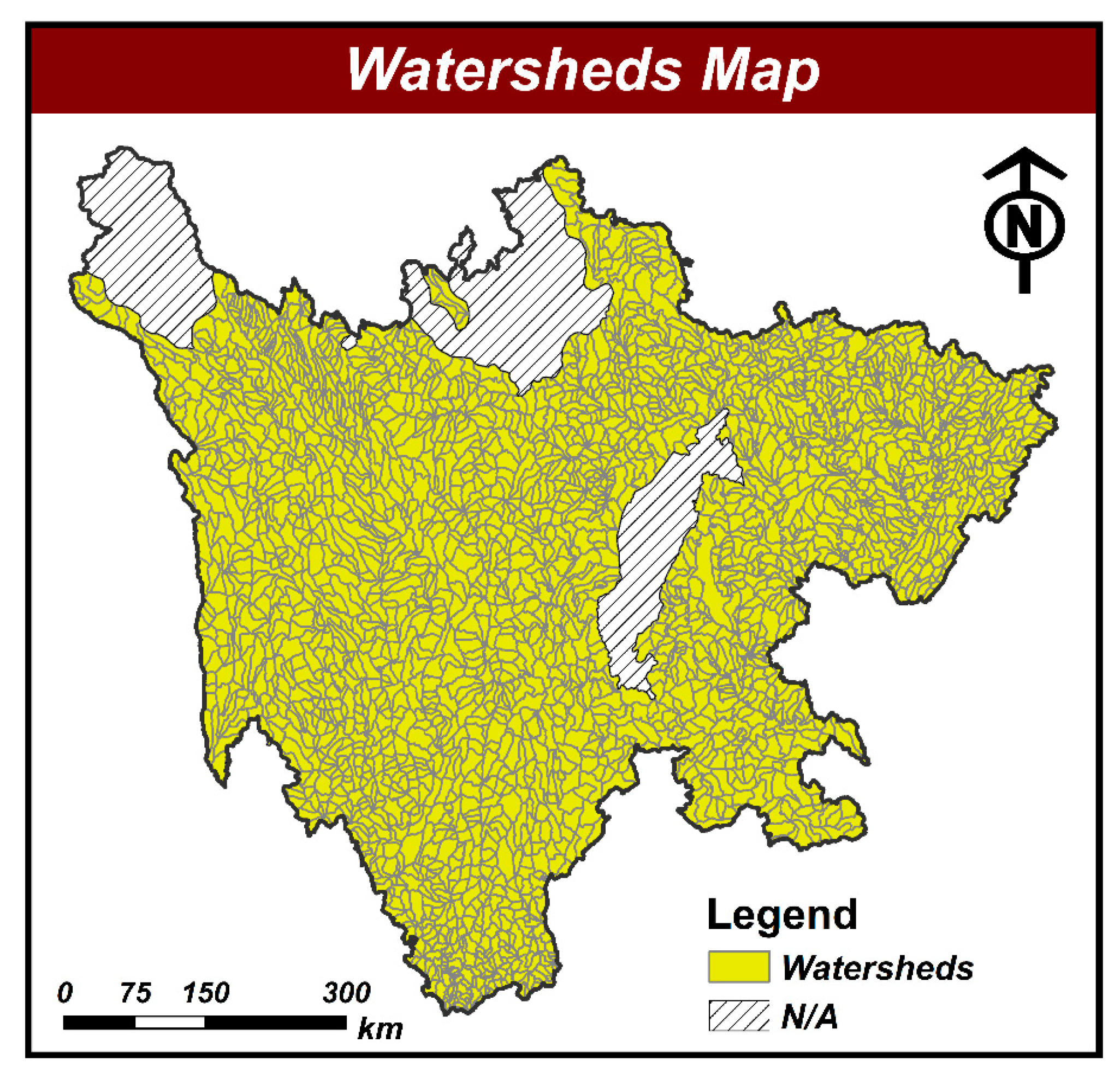
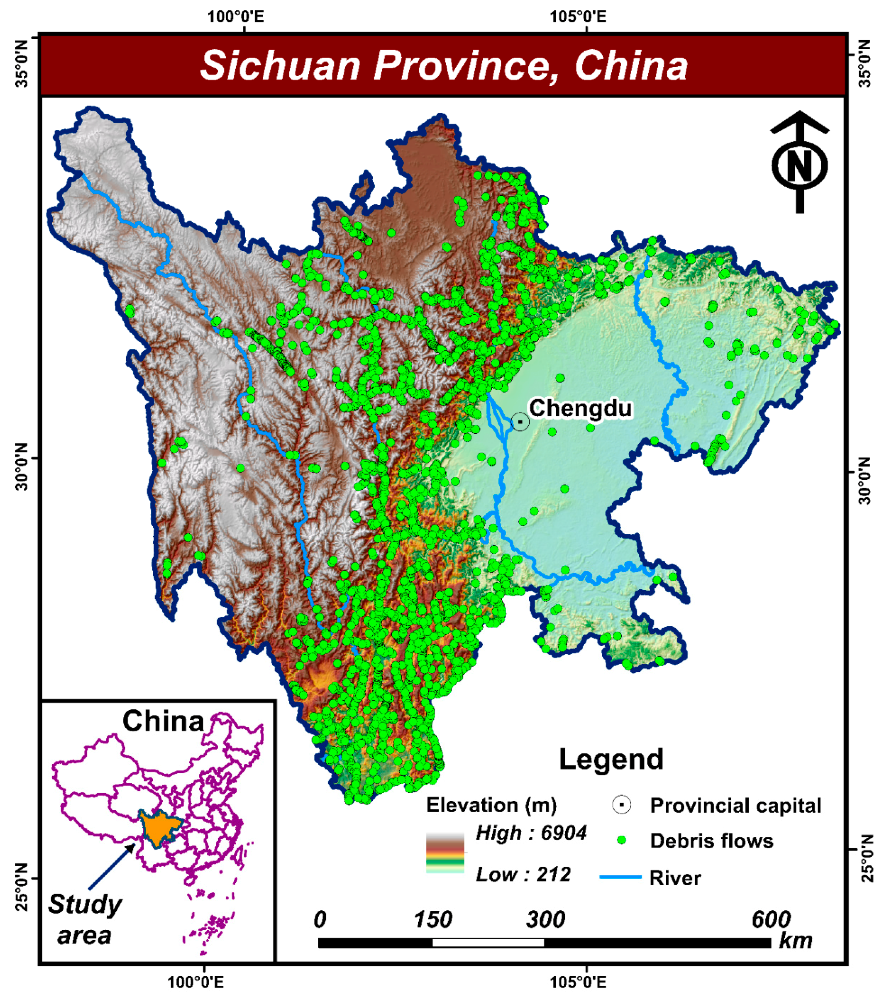
2. Study Area
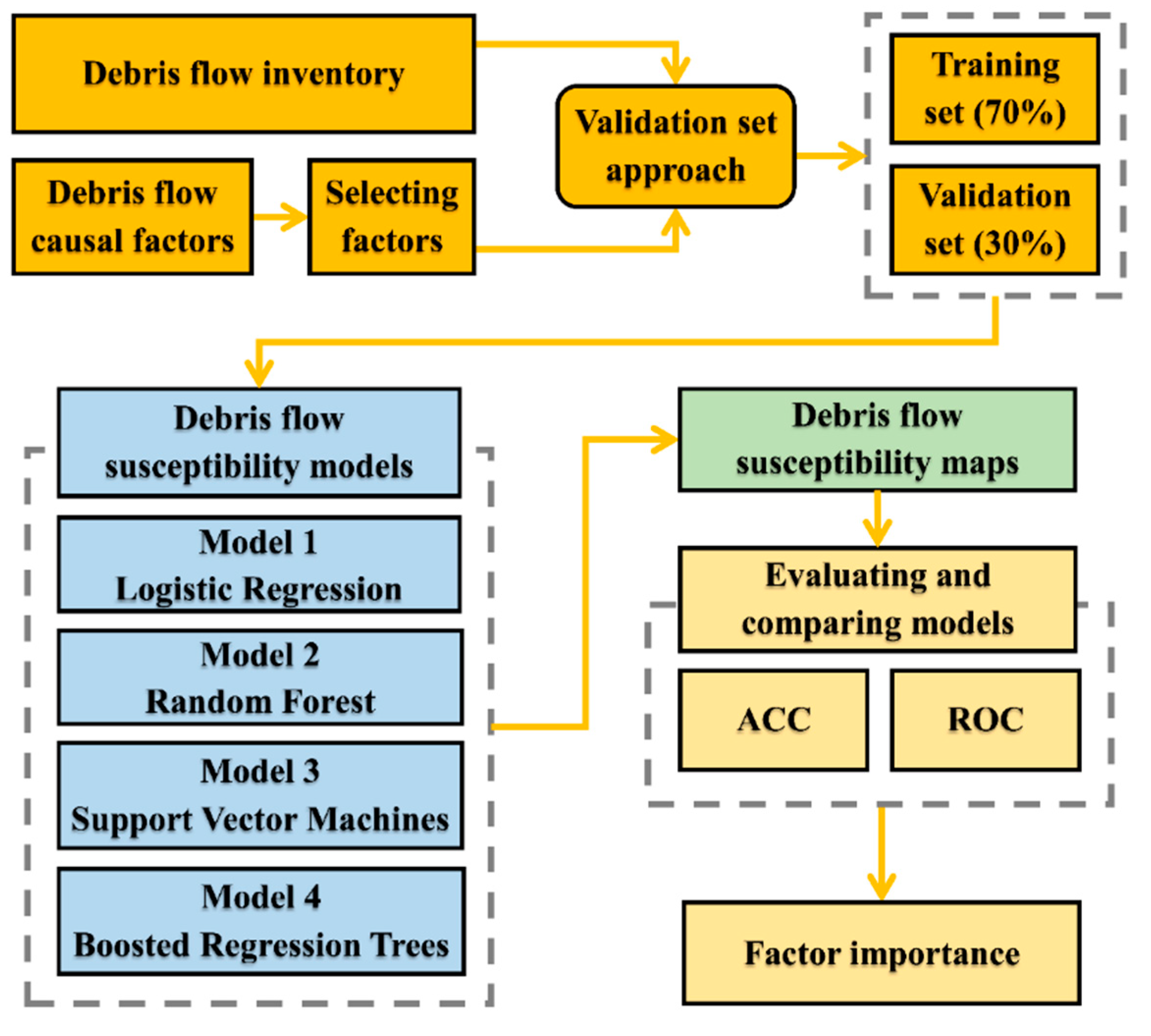
3. Materials and Methods
3.1. Preparation of Data Sets
3.1.1. Compilation of Debris Flow Inventory
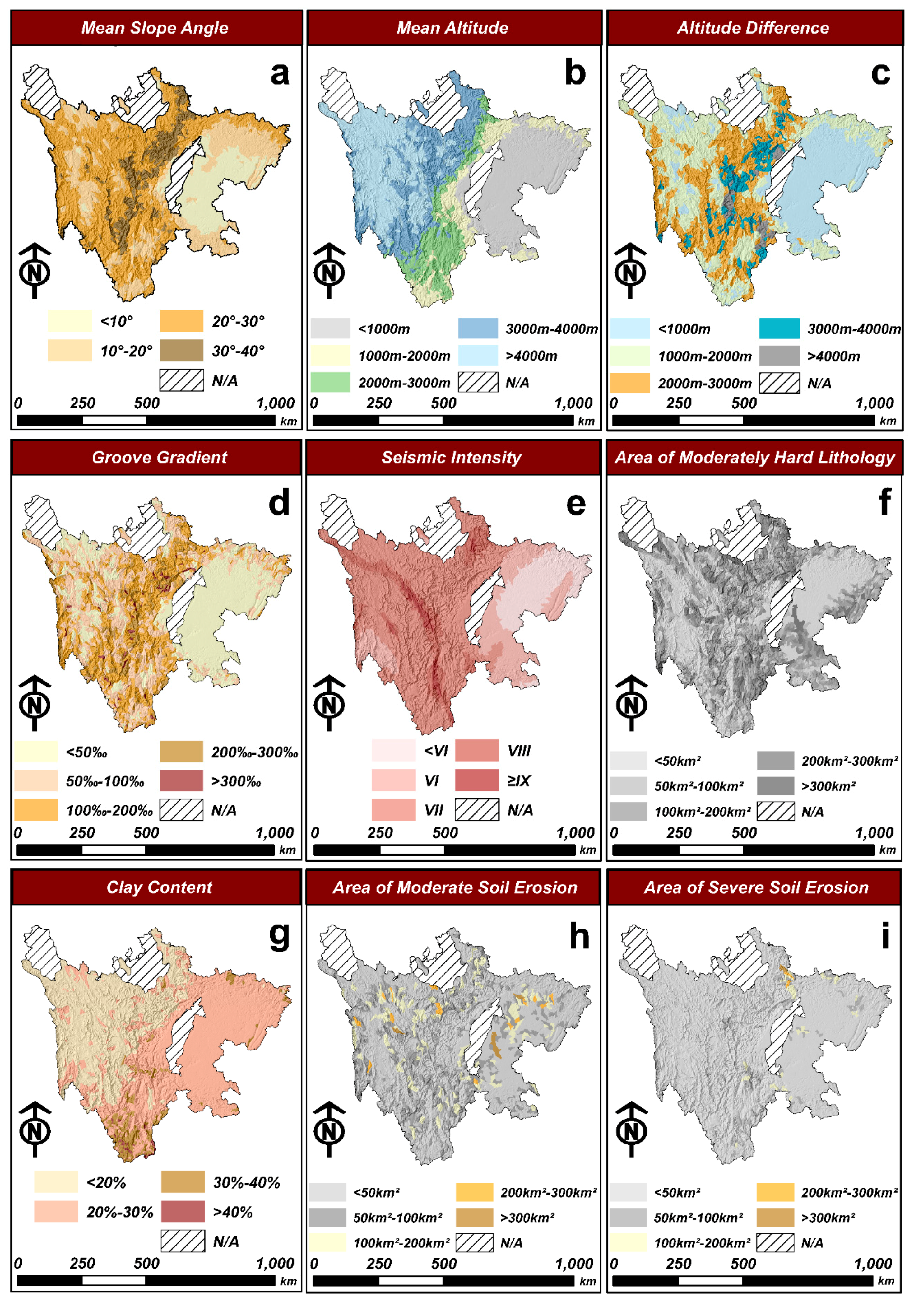
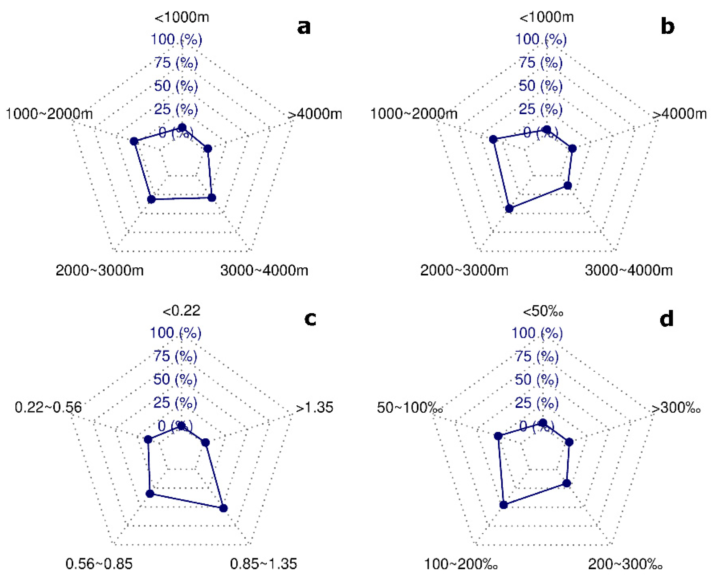
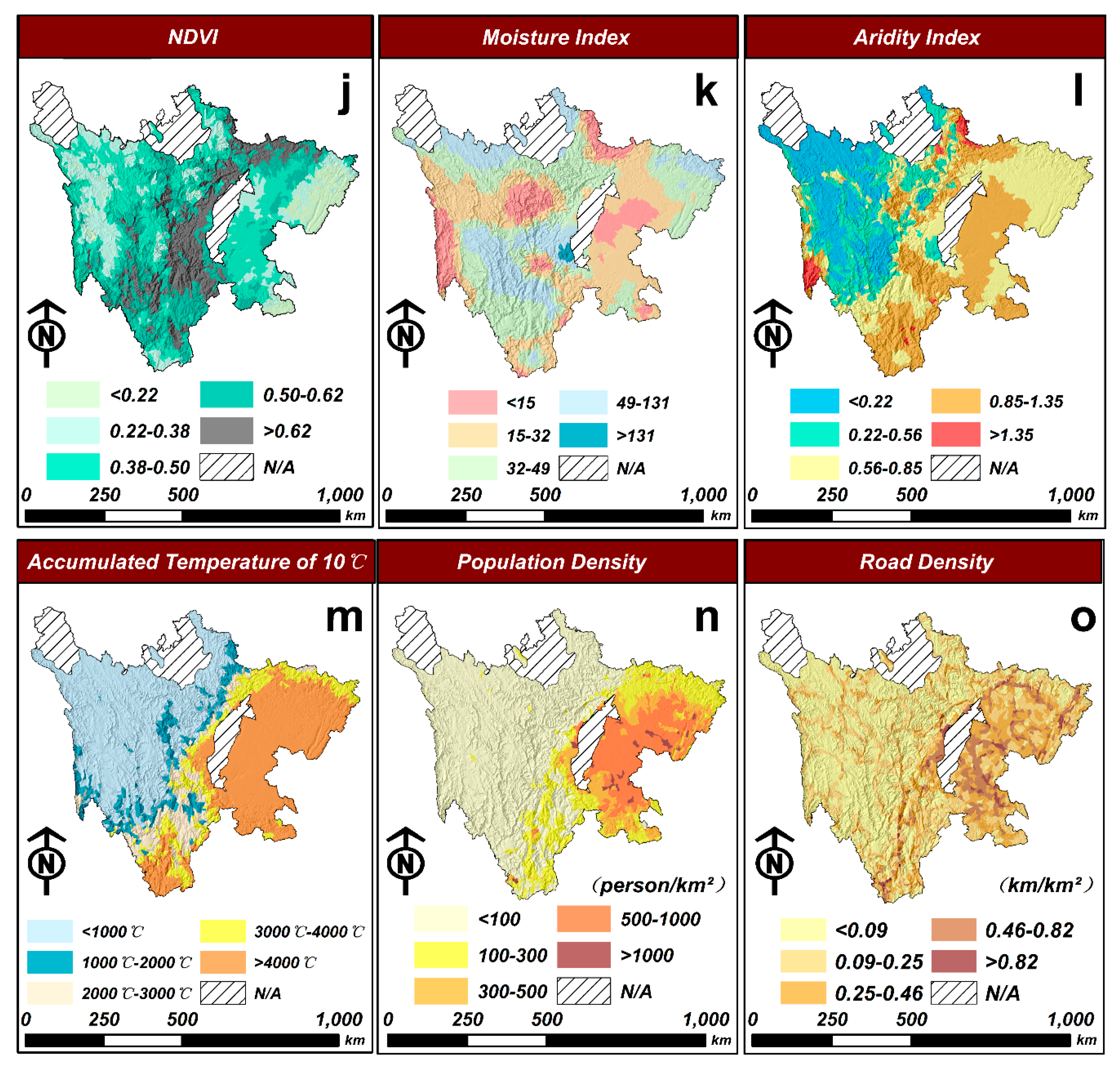
3.1.2. Selection of Debris Flow Causal Factors
3.1.3. Partition of Data Sets
3.2. Model Construction Using Machine Learning Algorithms
3.2.1. Logistic Regression (LR)
3.2.2. Random Forest (RF)
3.2.3. Support Vector Machines (SVM)
3.2.4. Boosted Regression Trees (BRT)
3.3. Evaluation and Comparison Methods
4. Results
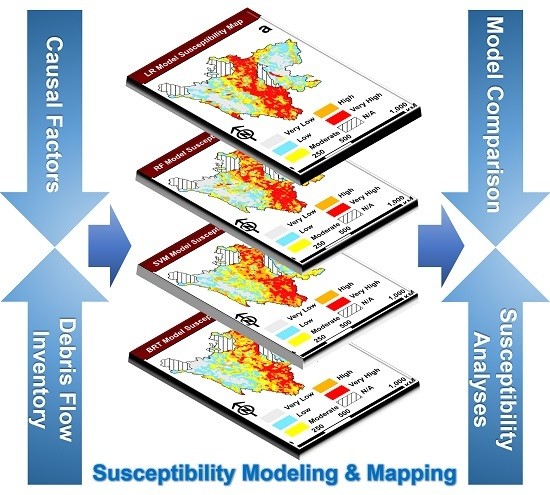
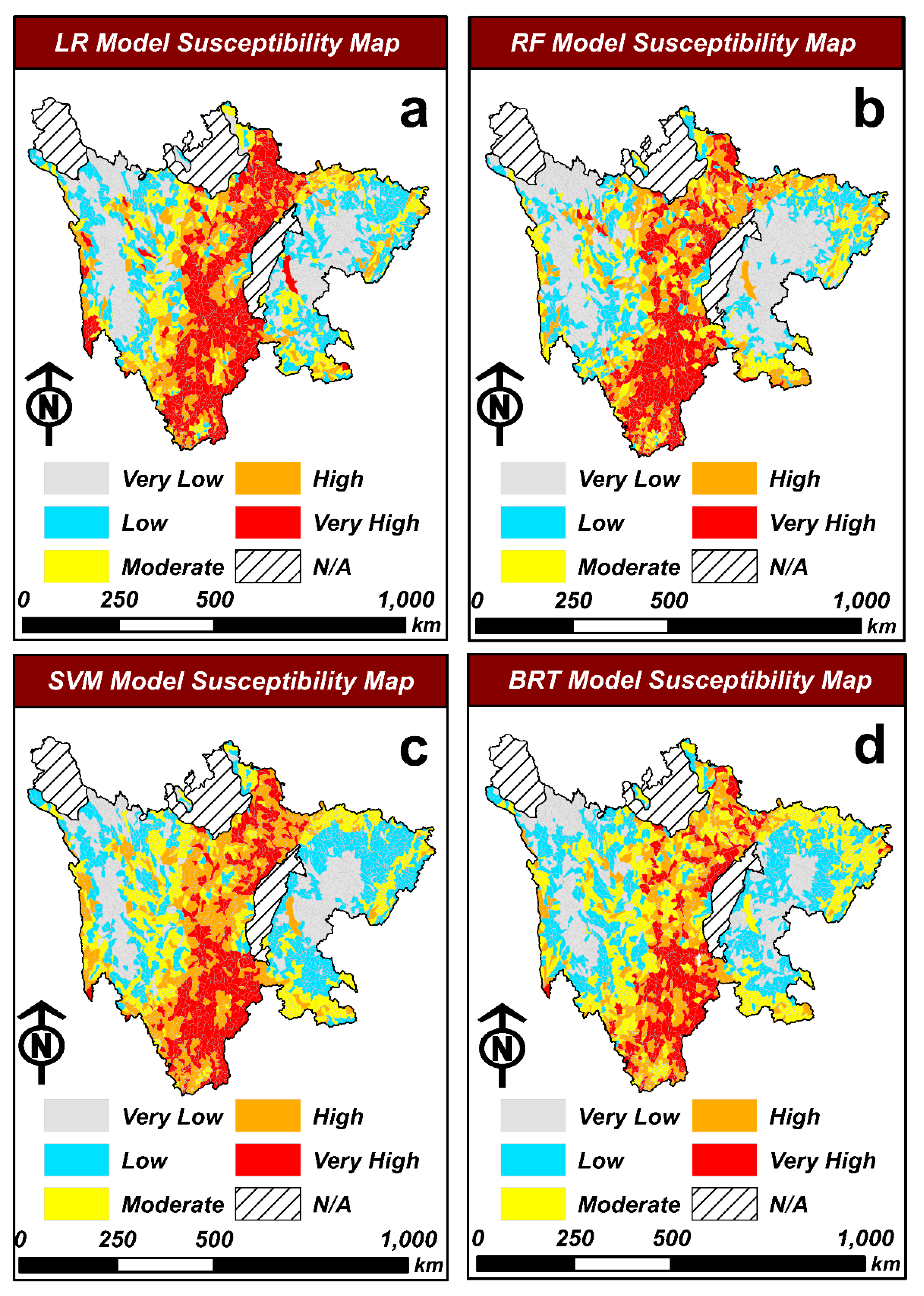
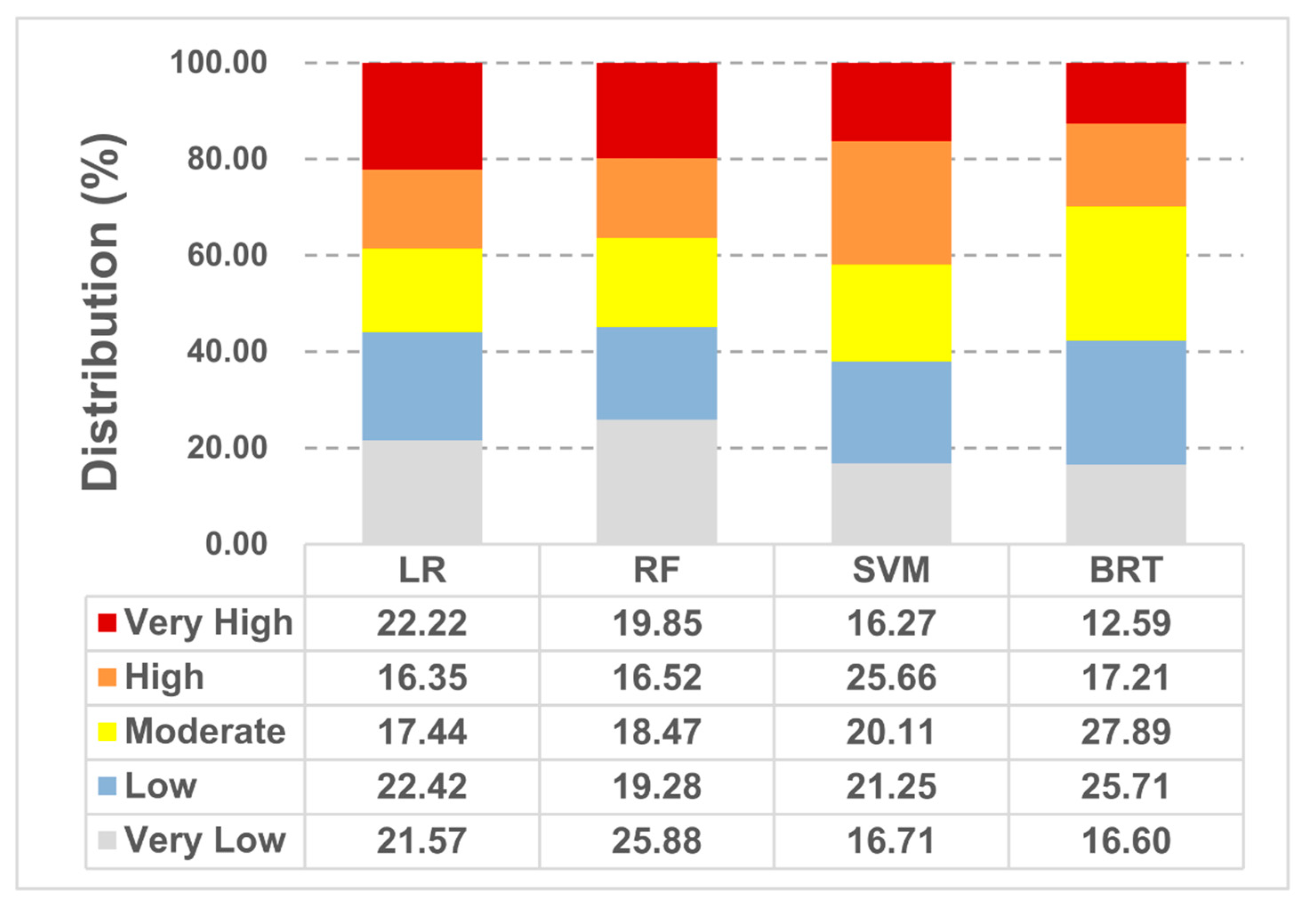
4.1. Development of Debris Flow Susceptibility Maps
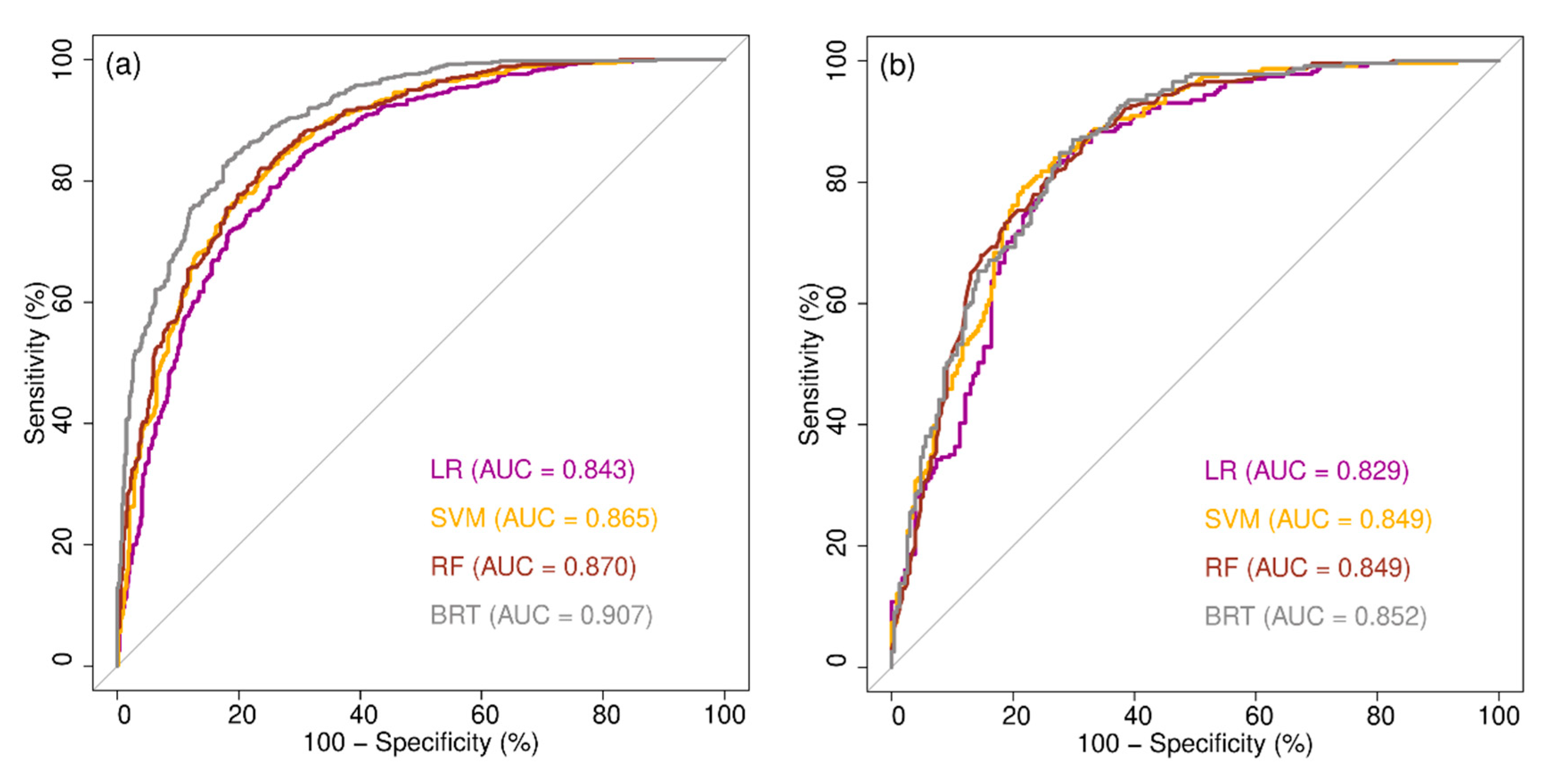
4.2. Evaluation and Comparison of Machine Learning Models
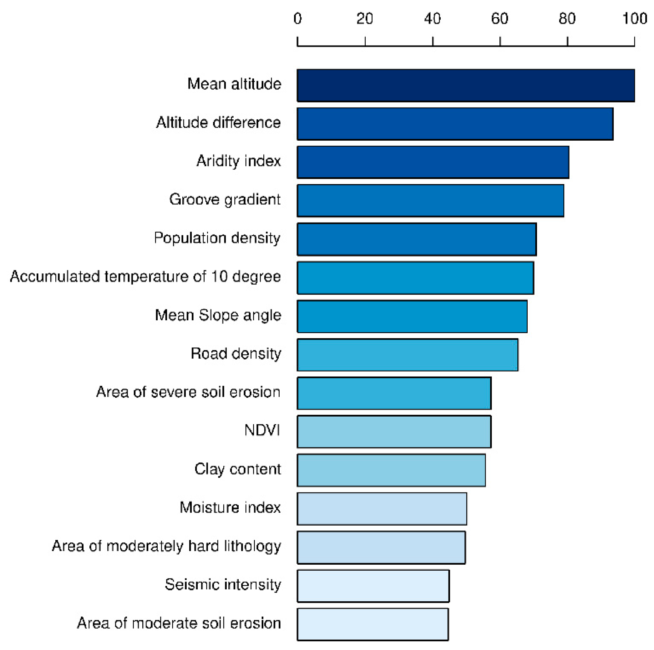
4.3. Assessment of Factor Importance
5. Discussion
6. Conclusions
Author Contributions
Funding
Conflicts of Interest
References
- Simoni, S.; Zanotti, F.; Bertoldi, G.; Rigon, R. Modelling the probability of occurrence of shallow landslides and channelized debris flows using GEOtop-FS. Hydrol. Process. 2008, 22, 532–545. [Google Scholar] [CrossRef]
- Kang, S.; Lee, S.-R. Debris flow susceptibility assessment based on an empirical approach in the central region of South Korea. Geomorphology 2018, 308, 1–12. [Google Scholar] [CrossRef]
- Liu, X.; Miao, C.; Guo, L. Acceptability of debris-flow disasters: Comparison of two case studies in China. Int. J. Disaster Risk Reduct. 2019, 34, 45–54. [Google Scholar] [CrossRef]
- Zhong, D.; Xie, H.; Wei, F. Comprehensive Regionalization of Debris Flow Risk Degree in the Upper Yangtze River, 1st ed.; Scientific and Technical Publishers: Shanghai, China, 2010; ISBN 978-7-5478-0103-1. [Google Scholar]
- Di, B.; Chen, N.; Cui, P.; Li, Z.L.; He, Y.P.; Gao, Y.C. GIS-based risk analysis of debris flow: An application in Sichuan, southwest China. Int. J. Sediment Res. 2008, 23, 138–148. [Google Scholar] [CrossRef]
- Tang, C.; Van Asch, T.; Chang, M.; Chen, G.; Zhao, X.; Huang, X. Catastrophic debris flows on 13 August 2010 in the Qingping area, southwestern China: The combined effects of a strong earthquake and subsequent rainstorms. Geomorphology 2012, 139, 559–576. [Google Scholar] [CrossRef]
- Brabb, E.E. Innovative Approaches to Landslide Hazard Mapping. In Proceedings of the Fourth International Symposium on Landslides, Canadian Geotechnical Society, Toronto, ON, Canada, 16–21 September 1984; pp. 307–324. [Google Scholar]
- Reichenbach, P.; Rossi, M.; Malamud, B.D.; Mihir, M.; Guzzetti, F. A review of statistically-based landslide susceptibility models. Earth Sci. Rev. 2018, 180, 60–91. [Google Scholar] [CrossRef]
- Blais-Stevens, A.; Behnia, P. Debris flow susceptibility mapping using a qualitative heuristic method and Flow-R along the Yukon Alaska Highway Corridor, Canada. Nat. Hazards Earth Syst. Sci. Discuss. 2015, 3, 3509–3541. [Google Scholar] [CrossRef]
- Hutter, K.; Svendsen, B.; Rickenmann, D. Debris flow modeling: A review. Contin. Mech. Thermodyn. 1994, 8, 1–35. [Google Scholar] [CrossRef]
- Aronica, G.T.; Cascone, E.; Randazzo, G.; Biondi, G.; Lanza, S.; Fraccarollo, L.; Brigandi, G. Assessment and mapping of debris flow hazard through integrated physically based models and GIS assisted methods. In Proceedings of the EGU General Assembly Conference Abstracts, Vienna, Austria, 2–7 May 2010; p. 13107. [Google Scholar]
- Schippa, L.; Pavan, S. Numerical modelling of catastrophic events produced by mud or debris flows. Int. J. Saf. Secur. Eng. 2011, 1, 403–422. [Google Scholar] [CrossRef]
- Liu, Y.; Di, B.; Zhan, Y.; Stamatopoulos, C.A. Debris Flows Susceptibility Assessment in Wenchuan Earthquake Areas Based on Random Forest Algorithm Model. Mt. Res. 2018, 36, 765–773. (In Chinese) [Google Scholar]
- Zhang, Y.; Ge, T.; Tian, W.; Liou, Y.-A. Debris Flow Susceptibility Mapping Using Machine-Learning Techniques in Shigatse Area, China. Remote Sens. 2019, 11, 2801. [Google Scholar] [CrossRef] [Green Version]
- Chang, T.-C.; Chao, R.-J. Application of back-propagation networks in debris flow prediction. Eng. Geol. 2006, 85, 270–280. [Google Scholar] [CrossRef]
- Pham, B.T.; Pradhan, B.; Bui, D.T.; Prakash, I.; Dholakia, M.B. A comparative study of different machine learning methods for landslide susceptibility assessment: A case study of Uttarakhand area (India). Environ. Model. Softw. 2016, 84, 240–250. [Google Scholar] [CrossRef]
- Roy, J.; Saha, S.; Arabameri, A.; Blaschke, T.; Bui, T.D. A Novel Ensemble Approach for Landslide Susceptibility Mapping (LSM) in Darjeeling and Kalimpong Districts, West Bengal, India. Remote Sens. 2019, 11, 2866. [Google Scholar] [CrossRef] [Green Version]
- Conoscenti, C.; Angileri, S.; Cappadonia, C.; Rotigliano, E.; Agnesi, V.; Märker, M. Gully erosion susceptibility assessment by means of GIS-based logistic regression: A case of Sicily (Italy). Geomorphology 2014, 204, 399–411. [Google Scholar] [CrossRef] [Green Version]
- Garosi, Y.; Sheklabadi, M.; Pourghasemi, H.R.; Besalatpour, A.A.; Conoscenti, C.; Oost, K.V. Comparison of differences in resolution and sources of controlling factors for gully erosion susceptibility mapping. Geoderma 2018, 330, 65–78. [Google Scholar] [CrossRef]
- Carrara, A.; Crosta, G.; Frattini, P. Comparing models of debris-flow susceptibility in the alpine environment. Geomorphology 2008, 94, 353–378. [Google Scholar] [CrossRef]
- Lee, S.; Park, I.; Choi, J.-K. Spatial Prediction of Ground Subsidence Susceptibility Using an Artificial Neural Network. Environ. Manag. 2012, 49, 347–358. [Google Scholar] [CrossRef]
- Cao, J.; Zhang, Z.; Wang, C.; Liu, J.; Zhang, L. Susceptibility assessment of landslides triggered by earthquakes in the Western Sichuan Plateau. CATENA 2019, 175, 63–76. [Google Scholar] [CrossRef]
- Xu, X.; Zhang, Y. Meteorological Datasets in China. Data Registration and Publishing System of Resource and Environment Science Data Center of Chinese Academy of Sciences. Available online: http://www.resdc.cn/DOI (accessed on 13 December 2017). (In Chinese).
- Xu, X. Spatial Distribution Datasets of Population in China. Data Registration and Publishing System of Resource and Environment Science Data Center of Chinese Academy of Sciences. Available online: http://www.resdc.cn/DOI (accessed on 11 December 2017). (In Chinese).
- Xu, X.; Liu, J.; Zhang, S.; Li, R.; Yan, C.; Wu, S. The Land Use and Land Cover Change Database in China. Data Registration and Publishing System of Resource and Environment Science Data Center of Chinese Academy of Sciences. Available online: http://www.resdc.cn/DOI (accessed on 2 July 2018). (In Chinese).
- Guzzetti, F.; Carrara, A.; Cardinali, M.; Reichenbach, P. Landslide hazard evaluation: A review of current techniques and their application in a multi-scale study, Central Italy. Geomorphology 1999, 31, 181–216. [Google Scholar] [CrossRef]
- Zhan, Y.; Luo, Y.; Deng, X.; Grieneisen, M.L.; Zhang, M.; Di, B. Spatiotemporal prediction of daily ambient ozone levels across China using random forest for human exposure assessment. Environ. Pollut. 2018, 233, 464–473. [Google Scholar] [CrossRef] [PubMed]
- Nefeslioglu, H.A.; Duman, T.Y.; Durmaz, S. Landslide susceptibility mapping for a part of tectonic Kelkit Valley (Eastern Black Sea region of Turkey). Geomorphology 2008, 94, 401–418. [Google Scholar] [CrossRef]
- Schicker, R.; Moon, V. Comparison of bivariate and multivariate statistical approaches in landslide susceptibility mapping at a regional scale. Geomorphology 2012, 161–162, 40–57. [Google Scholar] [CrossRef]
- Rahmati, O.; Tahmasebipour, N.; Haghizadeh, A.; Pourghasemi, H.R.; Feizizadeh, B. Evaluation of different machine learning models for predicting and mapping the susceptibility of gully erosion. Geomorphology 2017, 298, 118–137. [Google Scholar] [CrossRef]
- Arabameri, A.; Pradhan, B.; Rezaei, K.; Lee, C.-W. Assessment of Landslide Susceptibility Using Statistical- and Artificial Intelligence-Based FR–RF Integrated Model and Multiresolution DEMs. Remote Sens. 2019, 11, 999. [Google Scholar] [CrossRef] [Green Version]
- Team, R.C. R: A Language and Environment for Statistical Computing; R Foundation for Statistical Computing: Vienna, Austria, 2018; ISBN 3-900051-07-0. [Google Scholar]
- Greco, R.; Sorriso-Valvo, M.; Catalano, E. Logistic Regression analysis in the evaluation of mass movements susceptibility: The Aspromonte case study, Calabria, Italy. Eng. Geol. 2007, 89, 47–66. [Google Scholar] [CrossRef]
- Bai, S.-B.; Wang, J.; Lü, G.-N.; Zhou, P.-G.; Hou, S.-S.; Xu, S.-N. GIS-based logistic regression for landslide susceptibility mapping of the Zhongxian segment in the Three Gorges area, China. Geomorphology 2010, 115, 23–31. [Google Scholar] [CrossRef]
- Atkinson, P.; Massari, R. Generalised Linear Modelling of Susceptibility to Landsliding in the Central Apennines, Italy. Comput. Geosci. Comput. Geosci. 1998, 24, 373–385. [Google Scholar] [CrossRef]
- Breiman, L. Random Forests. Mach. Learn. 2001, 45, 5–32. [Google Scholar] [CrossRef] [Green Version]
- Micheletti, N.; Foresti, L.; Robert, S.; Leuenberger, M.; Pedrazzini, A.; Jaboyedoff, M.; Kanevski, M. Machine Learning Feature Selection Methods for Landslide Susceptibility Mapping. Math. Geosci. 2014, 46, 33–57. [Google Scholar] [CrossRef] [Green Version]
- Svetnik, V.; Liaw, A.; Tong, C.; Culberson, J.C.; Sheridan, R.P.; Feuston, B.P. Random Forest: A Classification and Regression Tool for Compound Classification and QSAR Modeling. J. Chem. Inf. Comput. Sci. 2003, 43, 1947–1958. [Google Scholar] [CrossRef] [PubMed]
- Archer, K.J.; Kimes, R.V. Empirical characterization of random forest variable importance measures. Comput. Stat. Data Anal. 2008, 52, 2249–2260. [Google Scholar] [CrossRef]
- Pourghasemi, H.R.; Kerle, N. Random forests and evidential belief function-based landslide susceptibility assessment in Western Mazandaran Province, Iran. Environ. Earth Sci. 2016, 75, 185. [Google Scholar] [CrossRef]
- Vapnik, V.N. The Nature of Statistical Learning Theory; Springer: Berlin/Heidelberg, Germnay, 1995; ISBN 0-387-94559-8. [Google Scholar]
- Xing, Z.; Xu, Q.; Tang, M.; Nie, W.; Ma, S.; Xu, Z. Comparison of two optimized machine learning models for predicting displacement of rainfall-induced landslide: A case study in Sichuan Province, China. Eng. Geol. 2017, 218, 213–222. [Google Scholar]
- Zhou, C.; Yin, K.; Cao, Y.; Ahmed, B.; Li, Y.; Catani, F.; Pourghasemi, H.R. Landslide susceptibility modeling applying machine learning methods: A case study from Longju in the Three Gorges Reservoir area, China. Comput. Geosci. 2018, 112, 23–37. [Google Scholar] [CrossRef] [Green Version]
- Kavzoglu, T.; Sahin, E.K.; Colkesen, I. Landslide susceptibility mapping using GIS-based multi-criteria decision analysis, support vector machines, and logistic regression. Landslides 2014, 11, 425–439. [Google Scholar] [CrossRef]
- Kavzoglu, T.; Colkesen, I. A kernel functions analysis for support vector machines for land cover classification. Int. J. Appl. Earth Obs. Geoinf. 2009, 11, 352–359. [Google Scholar] [CrossRef]
- Schapire, R.E. The Boosting Approach to Machine Learning: An Overview. In Nonlinear Estimation and Classification; Denison, D.D., Hansen, M.H., Holmes, C.C., Mallick, B., Yu, B., Eds.; Springer: New York, NY, USA, 2003; pp. 149–171. ISBN 978-0-387-21579-2. [Google Scholar]
- Mouton, A.; De Baets, B.; Goethals, P. Ecological relevance of performance criteria for species distribution models. Ecol. Model. 2010, 221, 1995–2002. [Google Scholar] [CrossRef]
- James, G.; Witten, D.; Hastie, T.; Tibshirani, R. An Introduction to Statistical Learning: With Applications in R; Springer: Berlin/Heidelberg, Germany, 2014; ISBN 1-4614-7137-0. [Google Scholar]
- Di, B.; Zhang, H.; Liu, Y.; Li, J.; Chen, N.; Stamatopoulos, C.A.; Luo, Y.; Zhan, Y. Assessing Susceptibility of Debris Flow in Southwest China Using Gradient Boosting Machine. Sci. Rep. 2019, 9, 12532. [Google Scholar] [CrossRef] [Green Version]
- Chiu, D.; Wei, Y. R for Data Science Cookbook, 1st ed.; Packt Publishing: Birmingham, UK, 2016; ISBN B01ET5I38M. [Google Scholar]
- Lee, S.; Ryu, J.-H.; Kim, I.-S. Landslide susceptibility analysis and its verification using likelihood ratio, logistic regression, and artificial neural network models: Case study of Youngin, Korea. Landslides 2007, 4, 327–338. [Google Scholar] [CrossRef]
- Kang, Z.; Lee, C.-F.; Ma, A.; Luo, J. Debris Flow Research in China, 1st ed.; Science Press: Beijing, China, 2004; ISBN 978-7-03-013800-2. [Google Scholar]
- Liu, C. Analysis on Genetic Model of Wenjiagou Debris Flows in Wenchuan Earthquake Area, Sichuan. Geol. Rev. 2012, 58, 709–716. [Google Scholar]
- Stamatopoulos, C.A.; Di, B. Analytical and approximate expressions predicting post-failure landslide displacement using the multi-block model and energy methods. Landslides 2015, 12, 1207–1213. [Google Scholar] [CrossRef]
- Chen, W.; Xie, X.; Wang, J.; Pradhan, B.; Hong, H.; Bui, D.T.; Duan, Z.; Ma, J. A comparative study of logistic model tree, random forest, and classification and regression tree models for spatial prediction of landslide susceptibility. CATENA 2017, 151, 147–160. [Google Scholar] [CrossRef] [Green Version]


| No. | Causal Factors | Clusters | Sources |
|---|---|---|---|
| 1 | Mean slope angle | Topographic | ASTER GDEM (Spatial resolution of 30 m × 30 m) (http://earthexplorer.usgs.gov) |
| 2 | Slope aspect | ||
| 3 | Mean altitude | ||
| 4 | Altitude difference | ||
| 5 | Groove gradient | ||
| 6 | Seismic intensity * | Geological | China seismic information (Scale of 1:4,000,000) (http://www.csi.ac.cn) |
| 7 | Lithology * | Lithological composition map of Sichuan Province (Scale of 1:200,000) (http://www.csi.ac.cn) | |
| 8 | Soil texture * | Edaphic | Spatial distribution datasets of soil texture in China (Spatial resolution of 1 km × 1 km) (http://www.resdc.cn) |
| 9 | Soil erosion * | Spatial distribution datasets of soil erosion in China (Spatial resolution of 1 km × 1 km) (http://www.resdc.cn) | |
| 10 | Moisture index (Calculated by Thornthwaite method) | Meteorological | Meteorological datasets in China (Spatial resolution of 500 m × 500 m) (http://www.resdc.cn) |
| 11 | Aridity index | ||
| 12 | Mean annual temperature | ||
| 13 | Accumulated temperature of 10 °C | ||
| 14 | Annual precipitation | ||
| 15 | Population density | Sociometric | Spatial distribution datasets of population in China (Spatial resolution of 1 km × 1 km) (http://www.resdc.cn) |
| 16 | Road density | OpenStreetMap Data (http://planet.openstreetmap.org) | |
| 17 | Normalized Difference Vegetation Index (NDVI) | Land cover | MODIS images (Spatial resolution of 500 m × 500 m) (https://modis.gsfc.nasa.gov) |
| 18 | Land use * | The land use and land cover change database in China (Spatial resolution of 1 km × 1 km) (http://www.resdc.cn) |
| Observed | Predicted | |
|---|---|---|
| Debris-Flow | Non-Debris-Flow | |
| Debris-flow | True positive (TP) | False negative (FN) |
| Non-debris-flow | False positive (FP) | True negative (TN) |
| Evaluation Criteria | Models | |||
|---|---|---|---|---|
| LR | RF | SVM | BRT | |
| ACC | 0.762 | 0.791 | 0.785 | 0.823 |
| AUC | 0.843 | 0.870 | 0.865 | 0.907 |
| Evaluation Criteria | Models | |||
|---|---|---|---|---|
| LR | RF | SVM | BRT | |
| ACC | 0.762 | 0.779 | 0.781 | 0.781 |
| AUC | 0.829 | 0.849 | 0.849 | 0.852 |
© 2020 by the authors. Licensee MDPI, Basel, Switzerland. This article is an open access article distributed under the terms and conditions of the Creative Commons Attribution (CC BY) license (http://creativecommons.org/licenses/by/4.0/).
Share and Cite
Xiong, K.; Adhikari, B.R.; Stamatopoulos, C.A.; Zhan, Y.; Wu, S.; Dong, Z.; Di, B. Comparison of Different Machine Learning Methods for Debris Flow Susceptibility Mapping: A Case Study in the Sichuan Province, China. Remote Sens. 2020, 12, 295. https://0-doi-org.brum.beds.ac.uk/10.3390/rs12020295
Xiong K, Adhikari BR, Stamatopoulos CA, Zhan Y, Wu S, Dong Z, Di B. Comparison of Different Machine Learning Methods for Debris Flow Susceptibility Mapping: A Case Study in the Sichuan Province, China. Remote Sensing. 2020; 12(2):295. https://0-doi-org.brum.beds.ac.uk/10.3390/rs12020295
Chicago/Turabian StyleXiong, Ke, Basanta Raj Adhikari, Constantine A. Stamatopoulos, Yu Zhan, Shaolin Wu, Zhongtao Dong, and Baofeng Di. 2020. "Comparison of Different Machine Learning Methods for Debris Flow Susceptibility Mapping: A Case Study in the Sichuan Province, China" Remote Sensing 12, no. 2: 295. https://0-doi-org.brum.beds.ac.uk/10.3390/rs12020295