Understanding Land Subsidence Along the Coastal Areas of Guangdong, China, by Analyzing Multi-Track MTInSAR Data

Abstract

Coastal areas are usually densely populated, economically developed, ecologically dense, and subject to a phenomenon that is becoming increasingly serious, land subsidence. Land subsidence can accelerate the increase in relative sea level, lead to a series of potential hazards, and threaten the stability of the ecological environment and human lives. In this paper, we adopted two commonly used multi-temporal interferometric synthetic aperture radar (MTInSAR) techniques, Small baseline subset (SBAS) and Temporarily coherent point (TCP) InSAR, to monitor the land subsidence along the entire coastline of Guangdong Province. The long-wavelength L-band ALOS/PALSAR-1 dataset collected from 2007 to 2011 is used to generate the average deformation velocity and deformation time series. Linear subsidence rates over 150 mm/yr are observed in the Chaoshan Plain. The spatiotemporal characteristics are analyzed and then compared with land use and geology to infer potential causes of the land subsidence. The results show that (1) subsidence with notable rates (>20 mm/yr) mainly occurs in areas of aquaculture, followed by urban, agricultural, and forest areas, with percentages of 40.8%, 37.1%, 21.5%, and 0.6%, respectively; (2) subsidence is mainly concentrated in the compressible Holocene deposits, and clearly associated with the thickness of the deposits; and (3) groundwater exploitation for aquaculture and agricultural use outside city areas is probably the main cause of subsidence along these coastal areas.

1. Introduction

Guangdong Province is located on the South China Sea coast and has the longest coastline of any province in China, approximately 4300 km. Along this coastline, several large agglomerations (e.g., the Pearl River Delta (PRD) and Chao Shan Plain (CSP)), harbors (Zhujiang, Zhanjiang, and Shantou), and a wide range of aquaculture and agricultural areas are clustered, controlling the primary economic activity and ecological environment. Over the past few decades, this coastline has experienced rapid growth in both population and economy. The PRD has undergone a shift from an agricultural-based economy to an industrial- and technological-based economy, making the PRD Asia’s fourth-largest economy [1,2]. To satisfy the needs of urban residents and export trade, an increasing amount of land is exploited through the expansion of aquaculture land use and reclamation of seashore. Among these exploitations, large-scale freshwater aquaculture has made Guangdong Province one of the top three aquaculture areas in China [3], which has contributed to the increasing aquaculture export. However, accumulated anthropogenic activities along the coastline have caused land subsidence, which is monitored by in situ and InSAR measurements [4,5,6,7,8,9,10,11]. As the majority of these measurements are focused on the PRD, deformation monitoring for the entire coastline of Guangdong Province is not available. Moreover, in addition to the direct damage caused by anthropogenic activities, continued coastal subsidence can also accelerate relative sea-level rise [12,13,14], groundwater salination [15], infrastructure damage [7]. Therefore, comprehensive monitoring over the whole Guangdong coastline is essential to help elucidate the spatial-temporal evolution of subsidence, and causal analysis is needed to uncover the mechanisms of subsidence. Doing so can potentially contribute to more effective prevention and mitigation of disasters and protection of the ecosystem and economy.

Preliminary subsidence monitoring along the Guangdong coastal area is focused on several primary cities, such as Zhanjiang [6], and is based on in situ measurements (Global positioning system (GPS) and leveling). However, in situ measurements are costly when the surveying area is large and can provide only point measurements, which can hinder the interpretation of subsidence patterns due to low spatial coverage. In contrast, the InSAR technique, a widely used method for deformation monitoring, can provide deformation measurements at a meter-scale spatial resolution with millimeter accuracy [16,17,18]. During the evolution of InSAR algorithms, multi-temporal InSAR (MTInSAR) techniques have been developed and successfully applied in large-scale deformation time series monitoring [9,16,19,20,21,22] due to their superiority over differential InSAR (DInSAR) in the suppression of spatial and temporal decorrelation and atmospheric effects.

By using the MTInSAR technique, a range of deformation monitoring results were generated and analyzed along the Guangdong coastal area, for example, land subsidence in Guangzhou [8,10,23], Shenzhen [9,11,24], Macau [5], and the Lianjiang Plain [7]. Although these studies have obtained 2D deformation, the interest areas are mainly concentrated over urban areas of the PRD, and these areas have steady backscatters. Areas outside the PRD are rarely monitored except for some in situ measurements.

In addition to the limitation of coverage, these studies have mainly focused on illustrating the effectiveness of MTInSAR methods, and only simple qualitative analyses of land subsidence causes were presented. For example, land subsidence in Guangzhou and Shenzhen was caused by subway construction [8,25], and building damage in Macau and Lianjiang Plain was due to land reclamation and groundwater exploitation [5,7]. The majority of these land subsidence events were related to anthropogenic activities that occurred in urban areas, such as subway excavation and seashore reclamation. However, as mentioned above, several activities outside urban areas are in progress, such as the extensive exploitation of agricultural and aquaculture lands, which is a common cause of large land subsidence. For example, centimeter-scale subsidence rates caused by groundwater exploitation for agricultural use in Indonesia [26,27], Mexico [28,29], and the Mekong Delta [30] have been reported. Nevertheless, land subsidence in aquaculture-dominated areas, which is dominant the Guangdong coastline, has received far less attention than land subsidence in agricultural-dominated areas [31,32]. Moreover, quantitative analysis between subsidence and land use is rarely conducted except for some qualitative analysis based on the visual interpretation of optical images [26,27,28,33]. Hence, quantitative analysis of land subsidence along the Guangdong coastal area can help us to gain a better understanding of subsidence causes and provide guidance for land planning. To fill these research gaps, the following tasks were conducted: (1) Two MTInSAR processing techniques, SBAS-InSAR and TCPInSAR, were adopted to generate the deformation along the whole Guangdong coastal area, with long-wavelength L-band images. The relative accuracy of InSAR results was validated within the overlapped areas of adjacent tracks, and the precision was validated by the collected GPS measurements. (2) The mechanism of land subsidence was analyzed with a focus on the quantitative relationship between land use and geology.

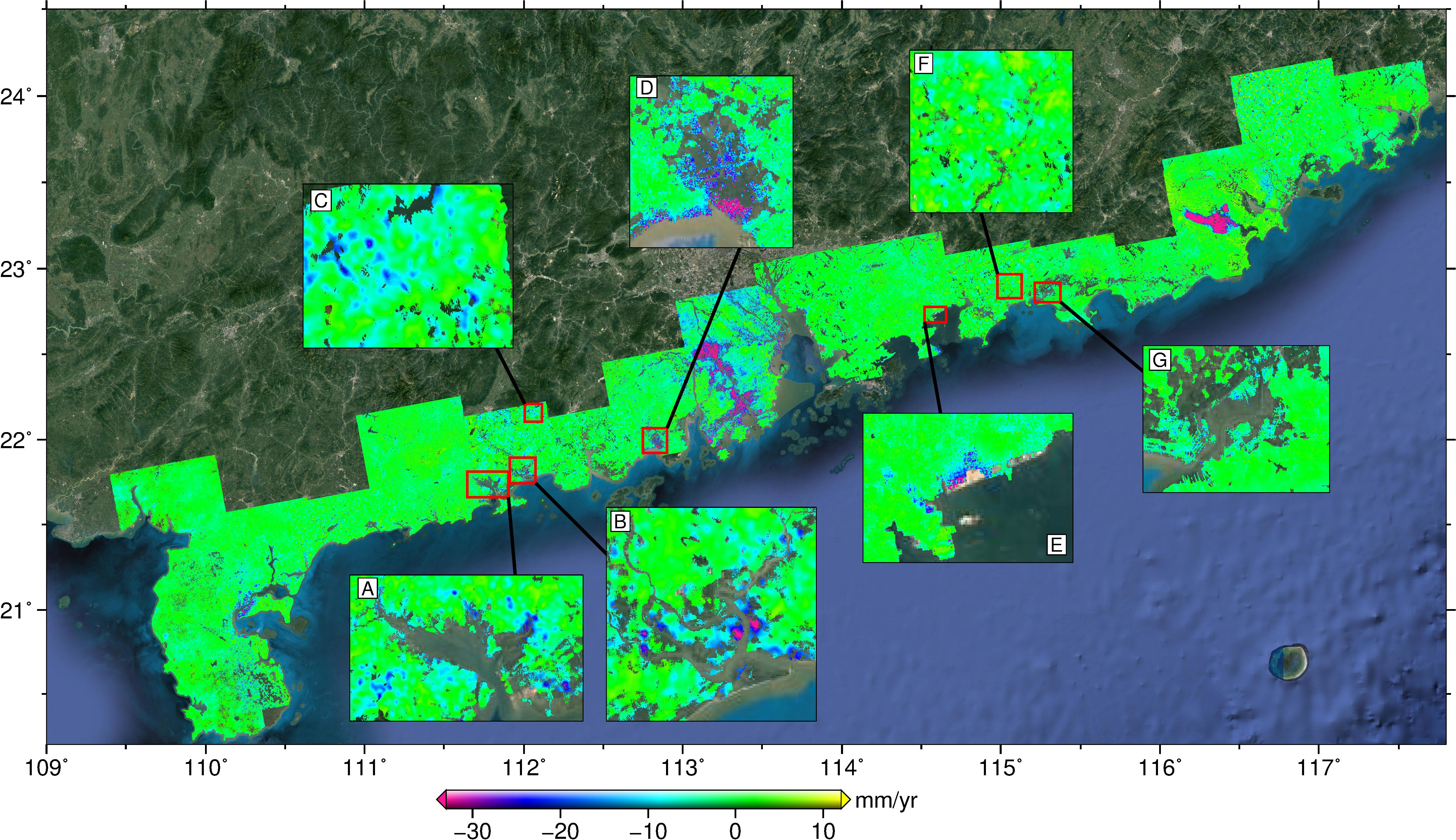
2. Geological Setting and Datasets

2.1. Geological Setting

Guangdong is bounded by the South China Sea to the south; the elevation of Guangdong decreases from north to south (Figure 1). In particular, in the coastal areas, the terrain is flat, with an average elevation of 101.2 m and a maximum elevation of 1493 m. Several major rivers, such as the Jianjiang River (JJR), Tanjiang River (TJR), Pearl River (PR), Hanjiang River (HJR), and Rongjiang River (RJR), flow across the coastal areas and merge into the sea (i.e., the cyan lines in Figure 2). Two deltas, the PRD and Chaoshan Plain (CSP), evolved from river valleys (the PR for the PRD; the HJR and RJR for the CSP) by sediment alluviation and land reclamation over tens of thousands of years. The coastal area has a humid subtropical climate, accompanied by frequent typhoons and heavy rainfall during July to October.

The Quaternary deposits are mainly distributed along the coastline and include four series: the Lower Pleistocene (Q1), Middle Pleistocene (Q2), Upper Pleistocene (Q3) and Holocene (Q4). The Holocene deposits are mainly concentrated in the PRD, CSP and Leizhou Peninsula (LZP), as marked by the light yellow shading in Figure 1. The sedimentary thickness of Q4 in the PRD ranges from 5 m to 60 m, as shown in Figure 2 [34]. The sedimentary thicknesses in LZP and CSP, ranging from 5 m to 40 m and 42 m to 132 m, respectively, are generated from the measurements of a series of boreholes [35,36,37,38,39], which are represented by black hollow circles in Figure 2.

2.2. Datasets

2.2.1. SAR Datasets and Landsat Datasets

To generate the surface motions of the whole Guangdong coastal area, we collected 253 archived SAR image datasets acquired from 2007 to 2011 by L-band ALOS1/PALSAR satellites, including 16 adjacent orbits covering an area of approximately 49,000 km² (represented by blue rectangles in Figure 1).

Table 1. SAR data and their imaging parameters.

Track_Frame	Polarization	Heading (°)	Incidence Angle (°)	Scenes	Time Span (yyyymmdd)	Master Image
452	HH	−10.5	38.7	18	20070713–20110308	20091018
453_450	HH	−10.6	38.7	5	20070614–20090201	20081217
453_460	HH	−10.6	38.7	5	20070730–20090201	20081217
454	HH	−10.5	38.7	13	20061229–20101009	20080101
455	HH	−10.5	38.7	7	20070115–20090120	20080118
456	HH	−10.5	38.7	15	20070201–20101228	20071220
457	HH	−10.6	38.7	8	20070706–20100714	20091011
458	HH	−10.6	38.7	14	20061205–20091213	20070723
459	HH	−10.6	38.7	22	20061222–20110102	20090211
460_430	HH	−10.6	38.7	21	20070711–20110119	20090716
460_440	HH	−10.6	38.7	12	20070711–20110119	20080111
461	HH	−10.6	38.7	19	20070125–20110205	20090802
462	HH	−10.6	38.7	7	20061227–20101122	20080214
463	HH	−10.6	38.7	8	20070113–20080718	20071016
464	HH	−10.6	38.7	15	20070130–20101226	20090622
465	HH	−10.6	38.7	9	20070216–20090106	20080104
466_410	HH	−10.6	38.7	9	20070305–20100729	20080723
466_400	HH	−10.7	38.7	13	20070305–20110129	20091211
467_390	HH	−10.6	38.7	11	20061220–20100630	20071223
467_400	HH	−10.6	38.7	11	20061220–20100630	20071223
467_410	HH	−10.6	38.7	11	20061220–20100630	20071223

gives the imaging parameters of each orbit, including the number, time span, and systematic parameters. An average of 12 acquisitions per frame was used during the 3.5-year period. In addition to the active remote sensing datasets, we also collected 8 optical Landsat images (represented by red dotted rectangles in Figure 1, see

Table 2. Landsat 8 data and their parameters.

Acquisition Time (yyyymmdd)	Cloud Content (%)	Path	Row
20131023	0.03	119	42
20131023	0.11	119	43
20130407	0.02	120	43
20131201	0.08	120	44
20131005	0.02	121	44
20141015	0.17	122	44
20131231	0.86	122	45
20150416	0.72	123	45
20141013	0.37	124	45
20131026	0.27	124	46

), aiming to generate land classification maps. Although a 2-year time span between SAR images and Landsat images exists, however, the changing rate of the agricultural land, forest land, and aquaculture land are only about 8.29%, 2.09%, and 2.99% respectively, according to the Statistics Bureau of Guangdong Province, see Table S1 [40]. Moreover, Landsat 8 image has a superior spectral resolution compared with Landsat 5 and 7, which is launched on 2013 [41,42].

2.2.2. In Situ Datasets

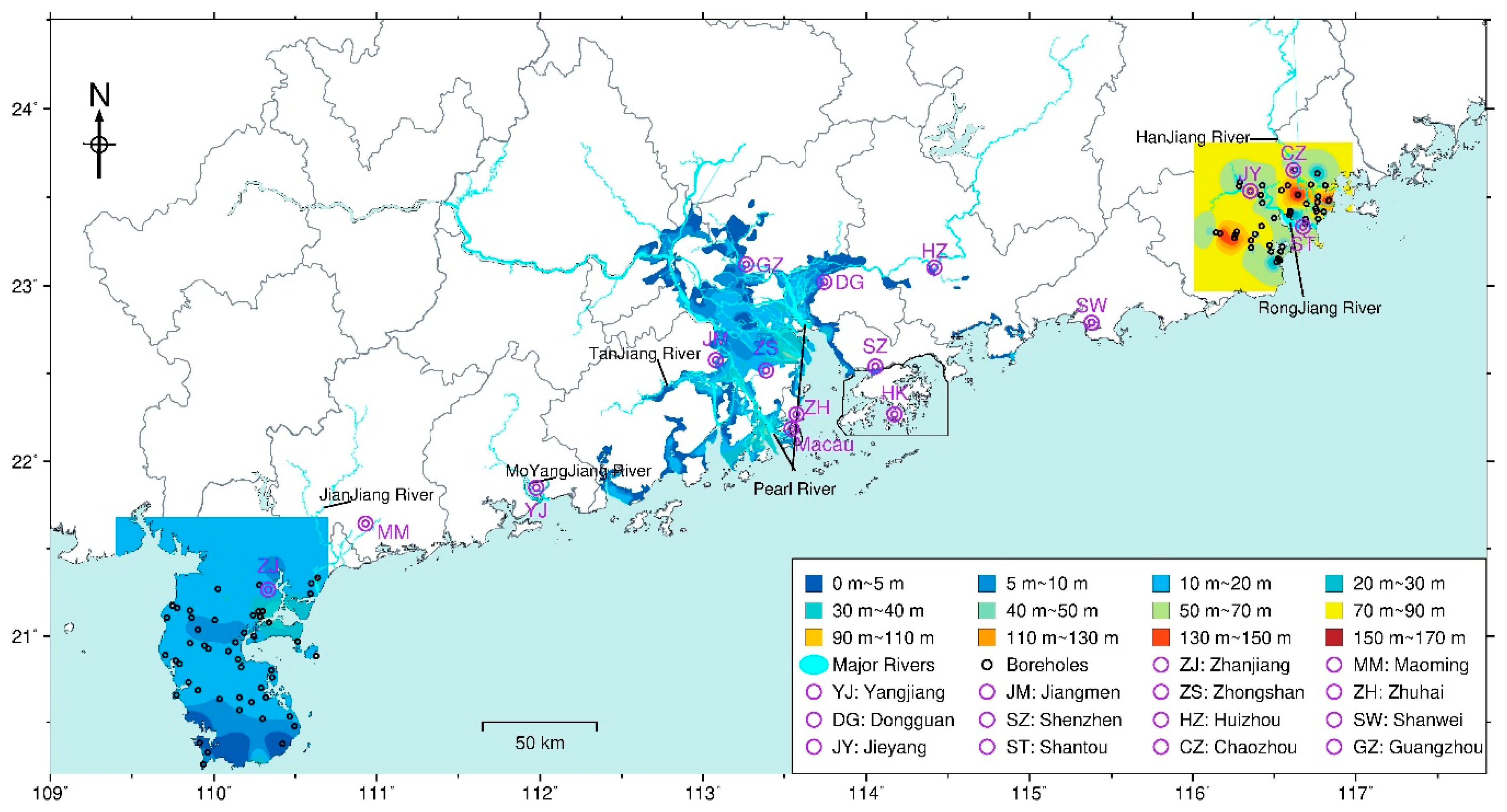
In addition to the remote sensing datasets, in situ datasets were collected in this study, including time-series datasets of 7 GPS stations and a dataset of Quaternary deposit thicknesses derived from boreholes (represented by black stars in Figure 1 and black circles in Figure 2, respectively). The GPS data were used to validate the InSAR-derived results, and the borehole data were adopted to generate the 2D deposit maps (Figure 2).

3. Methodology

MTInSAR is developed based on DInSAR, aiming to extract the deformation from mixed phases of series differential interferograms. That is, the residual topographic phase (${\phi }_{topo}$), deformation phase (${\phi }_{def}$), orbit phase (${\phi }_{orb}$), atmospheric phase (${\phi }_{aps}$) and noise (${\phi }_{noi}$) constitute the differential interferometric phase (${\phi }_{Dint}$).

$$W\left\{{\phi }_{Dint}\right\}=W\left\{{\phi }_{topo}+{\phi }_{def}+{\phi }_{orb}+{\phi }_{aps}+{\phi }_{noi}\right\}$$

(1)

where $W\left\{{\phi }_{Dint}\right\}$ is a phase wrap operation. To generate high-precision deformation rate and time-series, MTInSAR is mainly focus on the elimination of atmospheric phase and decorrelation noise based on wrapped or unwrapped phases. In this case, i.e., coastal areas with large coverage and serious temporal decorrelation, multi-master MTInSAR with a large multilooking number (3 and 8 looks in the range and azimuth directions, respectively) is adopted. Specifically, considering the complicated data conditions, such as frames with limited SAR image numbers and serious atmospheric effects in the coastal area, two kinds of MTInSAR are adopted. The first is SBAS-InSAR based on unwrapped phases, which is appropriate for most situations. The second method is an arc-based method, TCPInSAR, which is based on wrapped phases and aims to eliminate the influence of serious atmospheric effects. Considering the data processing efficiency, the latter is adopted in the case that the SAR image number is limited and the atmospheric effects are serious (tracks 453, 457, 462 and 463), see the comparison between pixel-based SBAS-InSAR and arc-based TCPInSAR in Figure S1. After generating deformation over the 16 orbits, the average velocity maps in the line of sight (LOS) direction are mosaiced after removing the relative offsets in the overlapped areas by a linear polynomial fitting [43], considering the approximate incident angle (38.7°, see Supplementary Table S1). Moreover, the precision of the InSAR results is evaluated, including relative precision calculation by the velocity difference in the overlapped area of adjacent orbits and analysis of the absolute precision with respect to GPS measurements. Next, the land-use classification maps along the coastal areas are obtained based on the selected optical Landsat images. Finally, the deformation features are observed, and the causes of the deformation are analyzed qualitatively and quantitatively. The flowchart is shown in Figure 3.

SBAS-InSAR, developed by Berardino et al. [16] and improved by researchers in recent years, is a pixel-based approach that has been widely used for wide-ranging deformation monitoring [16,26]. In this paper, GAMMA software is used to generate the unwrapped differential interferometric phases. SAR images of each track are first coregistered with a master image, as shown in Table 1. Interferograms with a given spatial and temporal baseline threshold (850 m and 800 days respectively), aiming to reduce the influence of decorrelation and digital elevation map (DEM) error on parameter estimation. After interferograms selection, traditional DInSAR with a multilook operation (three looks and eight looks in range and azimuth direction respectively) is applied to generate the unwrapped phases, including flatten and topographic phase removing, goldstein filtering, MCF phase unwrapping. The orbit error is removed with a polynomial fitting. Then, pixels with a mean coherence above 0.6 will be selected for the following processing procedures, including residual topographic estimation, atmosphere elimination, deformation time series calculation, and average velocity calculation. Here, we used a modified method to reduce the influence of residual topography caused by the correlation of the perpendicular baseline of ALOS1 in time dimension [44]. A spatial filtering and a temporal filtering are used to eliminate the atmosphere with a window-size of 500 m and two years respectively. A bootstrap with a parameter of 500 is adopted to generate the uncertainty of the average velocity fitting, and pixels whose uncertainty exceeds three times the standard deviation (std) are deleted. We also deleted those pixels whose coherent observation number is below two thirds of the total number.

Unlike SBAS-InSAR, TCPInSAR is a method proposed based on the wrapped phase of arcs [21,45,46]. It selected temporarily-coherence points (TCPs) and the unknown parameters, i.e., deformation rate, orbit phase, residual topographic phase, can be calculated without phase unwrapping operation. TCPInSAR proposed a local Delaunay networks with a uniform sampling in the range and azimuth directions, aiming to improve the arc density of the whole image. Unknown parameters are solved with an orbit errors joint model [46] and a phase ambiguity detection model [21] based on phase difference of arcs. Here, we used a sampling spacing of 700 m in both directions. The average velocity and residual topography of arcs are solved with an ambiguity detection method, that is, arcs with residuals over a given threshold are deleted (1.5 rad is used in this case). After generating the parameters of each arc, the parameters in each pixel are calculated based on an L1 norm least-squares estimation. The nonlinear deformation is obtained after spatial-temporal filtering for the residual phase. The final deformation time series is generated by combining the linear and nonlinear deformation.

Usually, 3D deformation, that is, deformation in both the vertical and horizontal directions, is calculated by the combination of ascending and descending images, which can help us infer hazard mechanisms. However, in this case, only descending SAR images were collected. Furthermore, according to the existing research, the horizontal deformation in the coastal areas is not obvious [47]. Hence, we assume that the horizontal displacement is negligible, deformation in the vertical direction can be generated with $d_v=d_{los}/cos\theta$, where $d_v$ and $d_{los}$ are the displacement in the vertical and LOS) directions, and $\theta$ is the incidence angle. The velocity values referred to in the following sections are in the LOS direction unless otherwise specified. In addition to the deformation monitoring techniques, an object-oriented nearest neighbor classification method based on multiresolution segmentation and supervised classification is also adopted for generating the land-use classification map. The details of the object classification method, which are beyond the scope of this study, can be found in previously published research [48]. As described in Section 2.2.1, because of the low change rate of land-use and the superiority of Landsat 8, the comparison between subsidence and land-use classification map is appropriate, which can help us understand the mechanism of land subsidence. The accuracy of the classification map is compared with a 30-m resolution product (with an overall accuracy of 97.29% within the range of [20°–30°N, 60°–120°E]) obtained in 2015 derived from the National Science & Technology Infrastructure of China [49,50]. The overall accuracy of the classification map in this study is about 89.5%.

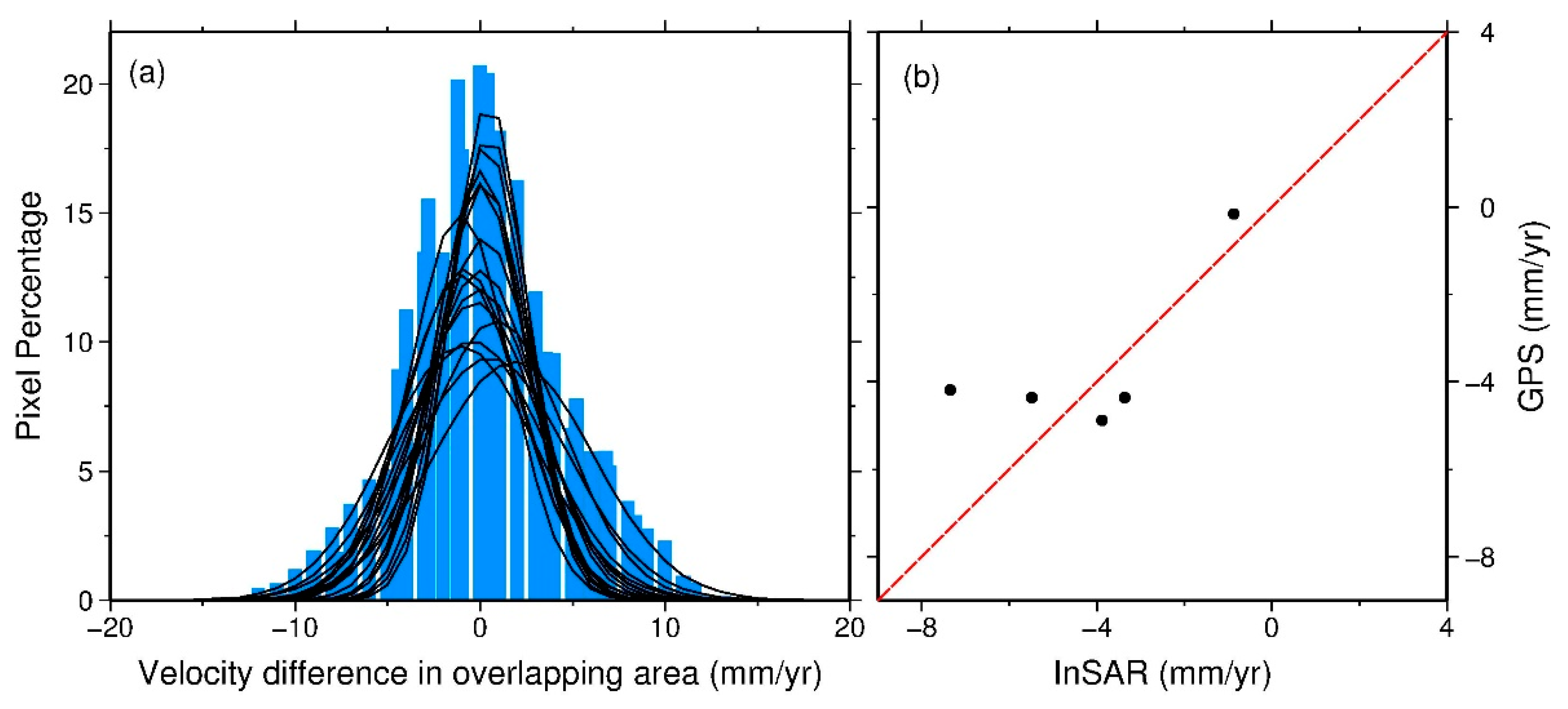
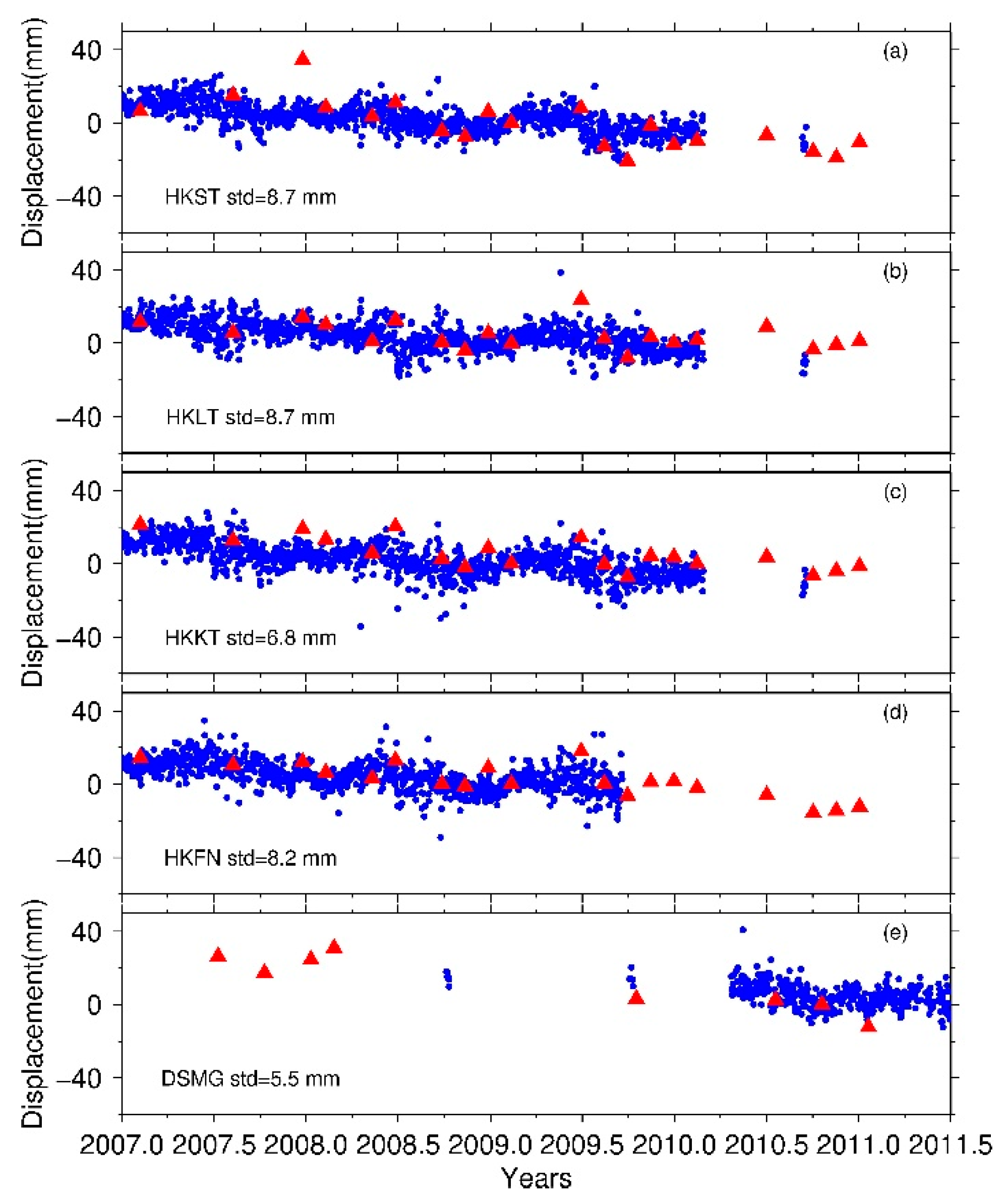
4. Validation of InSAR Results

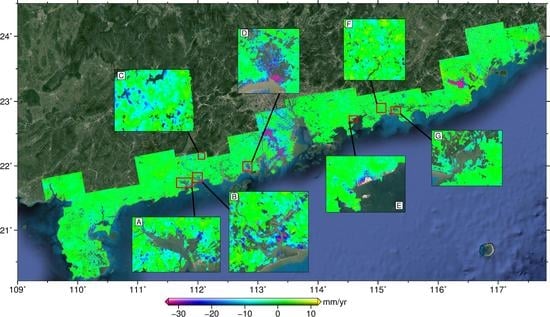
To quantitatively evaluate the accuracy of the InSAR-derived results, relative and absolute accuracy methods are adopted [51,52,53]. The former is also called inner precision, which is defined as the velocity difference in the overlapping areas of adjacent tracks, while the absolute accuracy is defined as the consistency with in situ measurements. Here, we used both methods to verify the deformation accuracy. Because the occurrence frequency of the large-scale terrain deformation in the coastal areas is very low, the relative accuracy is calculated by the velocity consistency in the overlapping areas between adjacent orbits after a 1^st order polynomial operation [43]. The histograms of the average velocity difference between adjacent orbits are shown in Figure 4, and the mean and std values are shown in

Table 3. Mean and standard deviation (std) of the average deformation rate difference in the overlapping areas of adjacent tracks.

Adjacent Tracks	Mean	Std	Adjacent Tracks	Mean	Std
T452-T453_450	−0.8	3.1	T460_430-T461	0.2	2.4
T452-T453_460	−0.9	3.1	T460_440-T461	1.8	4.3
T453_450-T454	−1.0	4.0	T461-T462	0.1	2.8
T453_460-T454	−0.4	3.9	T462-T463	−0.06	3.1
T454-T455	0.4	2.2	T463-T464	0.5	4.2
T455-T456	0.03	2.4	T464-T465	−0.02	2.4
T456-T457	−1.0	2.6	T465-T466	−0.1	3.3
T457-T458	0.3	2.2	T466-T467_390	−1.5	4.0
T458-T459	0.4	2.0	T466-T467_400	−0.2	3.4
T459-T460_440	0.8	3.6	T466-T467_410	−0.02	3.1

. It is obvious that the reference precision of velocity (std value of velocity difference) is generally less than 3.1 mm/yr, with the exception of several values approximate to 4 mm/yr. The causes of these high values may be the limited number of SAR images [54].

In addition to the statistical offsets in the overlapped areas, we also compared the velocity and deformation time series with the data collected from GPS stations, as shown in Figure 4b and Figure 5. It is noted that the velocity comparison between InSAR and GPS is in the vertical direction. The correlation of InSAR and GPS velocities is 0.71, confirming the high precision of InSAR results. Moreover, the std of deformation time series between the two measurements is also calculated, as shown in Figure 5. The GPS stations FOMO and HKSL are selected as reference stations in tracks 460 and 459 for the deformation time-series comparison, respectively, due to their different acquisition dates of SAR image series (see Table 1) and different coverage. The results show that the std of the deformation time series for stations DSMG, HKFN, HKKT, HKLT, and HKST are 5.5 mm, 8.2 mm, 6.8 mm 8.7 mm and 8.7 mm, respectively. The millimeter-level accuracy of the deformation series also proves the reliability of the InSAR-derived results.

5. Results

The surface displacement map of the Guangdong coastal areas derived from MTInSAR is calculated and shown in Figure 6. Positive values (yellow colors) represent movement toward the satellite (uplift). Negative values (purple colors) indicate movement away from the satellite (subsidence). Selected areas with concentrated land subsidence rates in excess of 20 mm/yr and discrete areas with gentle deformation are analyzed to grasp the features and characteristics of surface deformation. Three obvious subsidence areas in LZP, PRD, and CSP are identified. In addition, a land use classification map of the coastal areas of Guangdong Province is also generated and shown in Figure 7. Aquaculture, agriculture, urban, forest, and water are extracted based on the collected Landsat images.

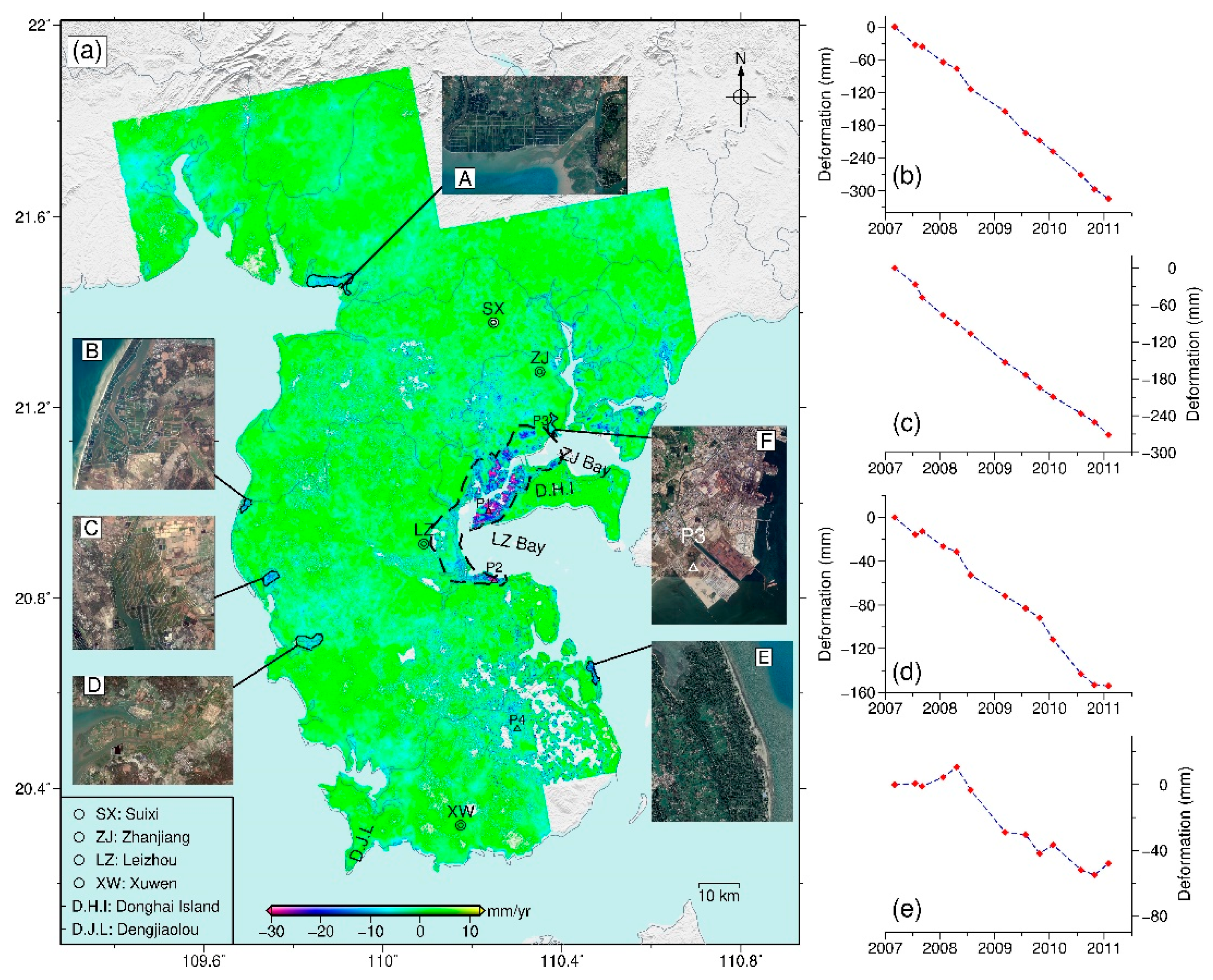
5.1. Subsidence in the Leizhou Peninsula

The LZP is located in southwest Guangdong Province. Crops are grown in more than 90% of the peninsula (see the yellow areas in Figure 7), making the LZP the granary for Guangdong Province. Following the SBAS-InSAR procedure, the result in the LZP is shown in Figure 8. The high subsidence (>20 mm/yr) in LZP is concentrated in the two bays (Zhanjiang Bay and Leizhou Bay) and the southwest of Donghai Island, as outlined by the black dotted circle in Figure 8. The subsidence area is approximately 251.5 km², with an average subsidence rate of 15.1 mm/yr, and the maximum subsidence rate of 58.0 mm/yr occurs on Donghai Island. The location of these subsidence bowls is consistent with the trend of middle groundwater decline [4]. In addition to the high rates of subsidence, some other subsidence bowls with areas over 4 km², located along the western coastline, are also observed. The corresponding optical images are also given, showing that obvious subsidence bowls are located in areas with aquaculture land use. Moreover, the deformation time-series of two selected points in aquaculture areas are shown in Figure 8b,c, with an approximately linear trend. Discrete subsidence with an average rate of 7.0 mm/yr is presented in inland LZP, such as the subsidence areas of Suixi and Leizhou, with a nonlinear deformation time-series trend, as shown in Figure 8e. In addition to subsidence in agricultural and aquaculture areas, small-scale displacement (with an average subsidence rate of 9.8 mm/yr) is also observed in urban areas of Zhanjiang city, especially in its industrial areas (see inset F in Figure 8a,d). In addition to the subsidence areas, a small-scale uplift (~3 mm/yr) is observed in Dengjiaolou, which is consistent with the results of traditional measurements from tectonic activity [47].

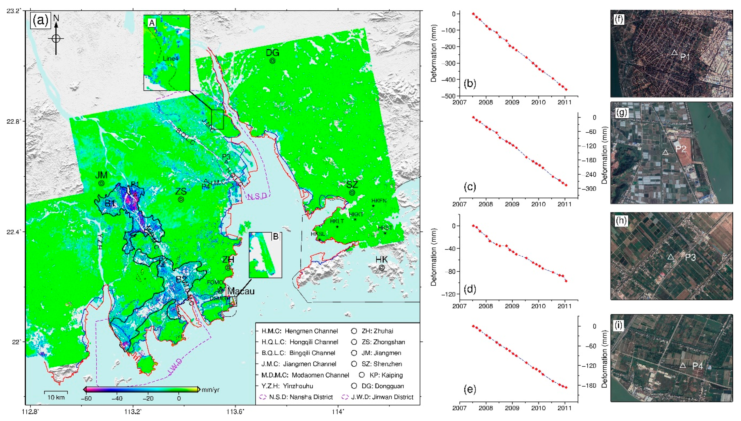
5.2. Subsidence in the Pearl River Delta

The spatial-temporal characteristic of subsidence in the PRD is much different in magnitude and range than that of the LZP, as shown in Figure 9. This result indicates that the large-scale subsidence areas with an average rate in excess of 35 mm/yr reach a total area of 263.37 km², in comparison to 15.16 km² in LZP during the approximate period. The subsidence area in the PRD is mainly distributed along the Pearl River tributary (see Figure 9). Two large-scale subsidence bowls are observed along the Modaomen channel (outlined by B1 and B2 in Figure 9), with average subsidence rates of 32.0 mm/yr and 25.1 mm/yr, respectively, and areas of 265.43 km² and 387.32 km², respectively. The statistical area is calculated after kriging interpolation due to the temporal decorrelation of the surrounding water. Subsidence bowls with low subsidence rates are also observed along the other three channels: the Hengmen channel, Bingqili channel, and Jiaomen channel. In addition, local subsidence areas with notable rates are distributed along the coastline, especially in reclamation areas (which are outlined between the blue and red lines during the period from 1984 to 2011 in Figure 9). For example, an artificial island located in Nansha district and a reclamation area located in Jinwan district (see dotted purple circles in Figure 9), have maximum subsidence rates of 71.9 mm/yr and 150.9 mm/yr, respectively. Notably, some small-scale uplift is found in mountainous areas (see the black dotted circles in Figure 9). This uplift may be caused by elevation-related atmospheric effects or residual topography. Besides the average deformation map, deformation time-series of four selected points are also generated (see Figure 9b–e). The linear trend is found in both agricultural and aquaculture areas (see Figure 9f–i).

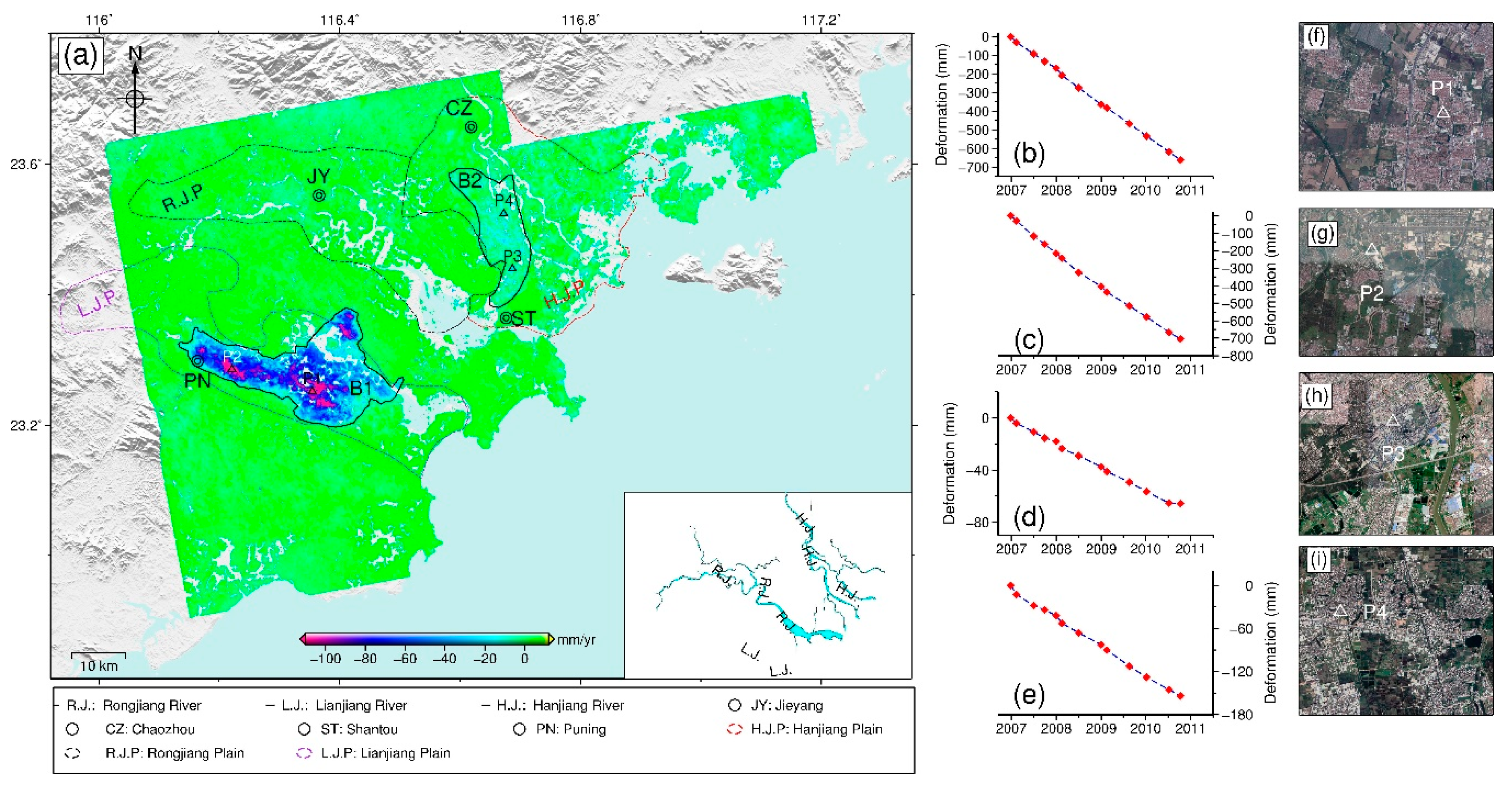
5.3. Subsidence in the Chaoshan Plain

The CSP consists of three river alluvial plains, the Lianjiang River Plain (LJP), Rongjiang River Plain (RJP) and Hanjiang River Plain (HJP), represented by purple, black and red dotted circles in Figure 10, respectively. The total area of these plains reaches 2600 km². The displacement results in the CSP are presented in Figure 10 and exhibit a specific spatial-temporal subsidence feature that, compared with the results of LZP and PRD, is very large and intensive. As shown in Figure 10, a large-scale subsidence bowl with an obvious boundary is observed in the LJP, outlined by B1. The area and average subsidence rate are 342.21 km² and 41 mm/yr, respectively. The maximum subsidence rate reaches 157.2 mm/yr. In addition to the subsidence in the LJP, some discrete small-scale subsidence areas are observed in the HJP and are marked by black circles in Figure 10, i.e., B2. The subsidence is mainly concentrated along the western side of the HJP, and the maximum subsidence rate reaches 32.9 mm/yr. In the RJP, a small subsidence area is also generated in Jieyang city, with a maximum subsidence rate of 24.2 mm/yr. Moreover, four points located in the mixed agricultural and urban areas (see Figure 10f–i) are selected to generate the deformation time-series, as shown in Figure 10b–e. The linear trend of the deformation time-series is also found.

5.4. Subsidence in Other Coastal Areas

In addition to the three selected subsidence areas, other subsidence areas are distributed discretely along the coastline, especially in river estuaries, for example, Hailing Bay and the estuary of the Moyang River in track 463, represented by the insets A and B in Figure 6, respectively, the estuary of Guanghai Bay in track 461 (see inset D in Figure 6), and the estuary of the Huangjiang River in track 456 (inset G in Figure 6). In addition to the subsidence occurring along the river system, some local subsidence is also observed in forest areas, such as the discrete subsidence bowls in tracks T463 and T457 (see the insets C and F in Figure 6). Moreover, elongated subsidence located in the industrial petrochemical region is also observed in track 458 (see inset E in Figure 6).

6. Discussion

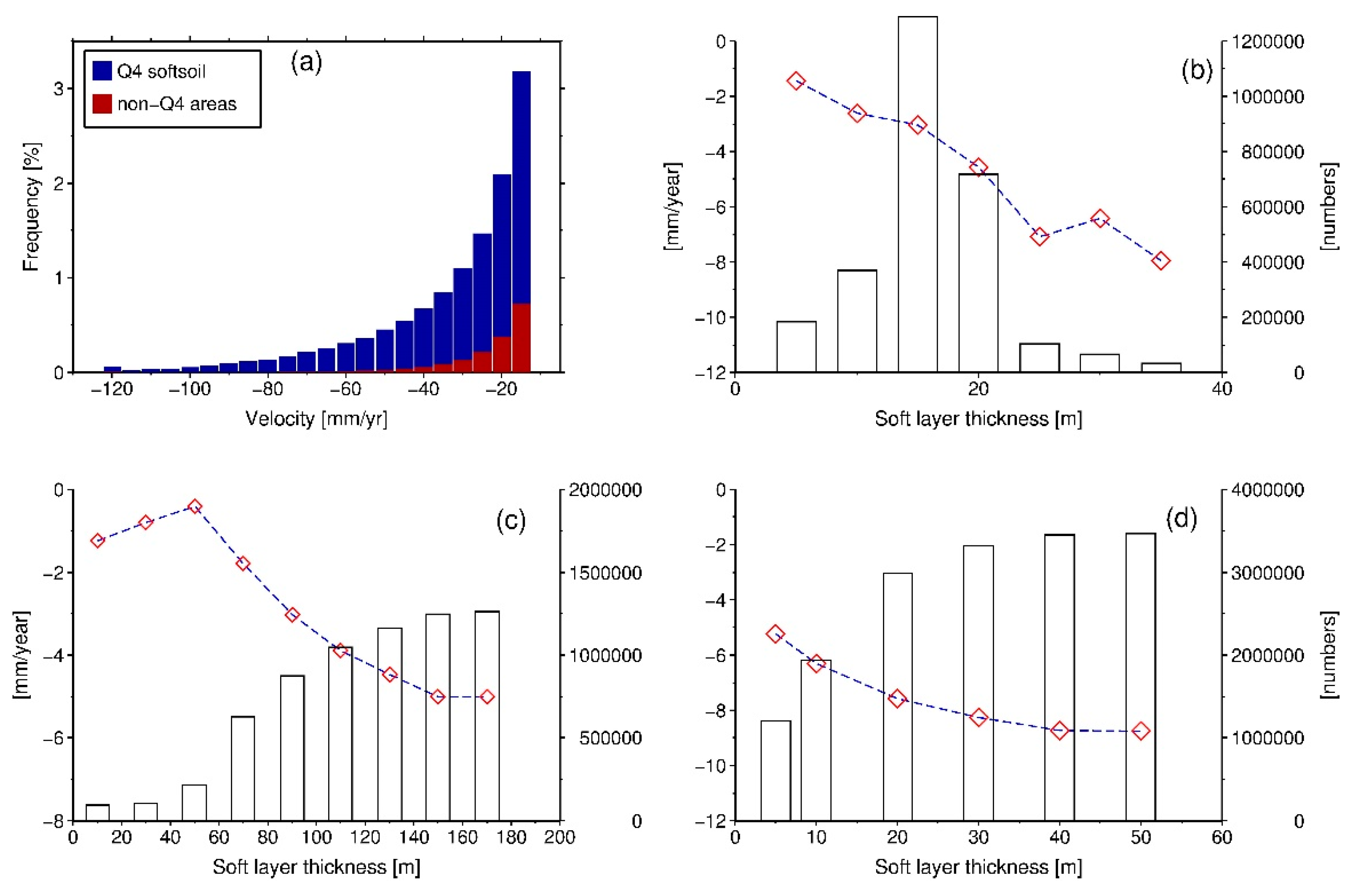
6.1. A positive Correlation between Sedimentary Thickness and Subsidence

We focused on a geological formation that is usually prone to natural hazards, namely, the Holocene series (Q4), to investigate the correlation of these two factors. As shown in Figure 1, in addition to some discrete distribution along the coastline, Q4 is mainly distributed in the LZP, PRD, and CSP. The areas of subsidence have a distribution similar to that of the Q4 deposits, especially in areas with notable subsidence rates. To clearly analyze this similarity, we calculated the histograms of the subsidence rate (>15 mm/yr) within and out of areas with Q4 deposits; the results are shown in Figure 11a. The percentage along the Y axis is calculated by the following equations:

$$\begin{gathered} {Rer}_{Q4}=\frac{\mathit{pixel} \mathit{number} \mathit{whose} \mathit{subsidence} \mathit{rate}>15\mathrm{mm}/\mathrm{yr} \mathit{within} Q4 \mathit{area}}{\mathit{sum} \mathit{total} \mathit{pixel} \mathit{number} \mathit{within} Q4 \mathit{area}} \\ {Rer}_{no-Q4}=\frac{\mathit{pixel} \mathit{number} \mathit{whose} \mathit{subsidence} \mathit{rate}>15\mathrm{mm}/\mathrm{yr} \mathit{out} \mathit{of} Q4 \mathit{area}}{\mathit{sum} \mathit{total} \mathit{pixel} \mathit{number} \mathit{out} \mathit{of} Q4 \mathit{area}} \end{gathered}$$

(2)

Subsidence is mainly located within the Q4 area, especially in areas with subsidence rates higher than 40 mm/yr (see the blue columns in Figure 11a).

To quantitatively analyze the correlation of these two factors, we also considered the thickness of Q4 deposits in the LZP, PRD, and CSP (see the Q4 depth map in Figure 2). The Q4 thickness maps of the LZP and CSP are generated by a kriging interpolation based on the depths collected from borehole measurements, which are represented by black circles [55]. We divided the thickness of Q4 into several sections, for example, 0 m to 10 m with an interval of 5 m, 10 m to 50 m with an interval of 10 m, and 50 m to 170 m with an interval of 20 m. Additionally, we calculated the average subsidence rate in these sections across the LZP, CSP and PRD. These results are represented by red diamonds in Figure 11b–d, respectively. We can see that an obvious positive correlation between Q4 thickness and subsidence rate is observed, that is, the greater the thickness is, the higher the subsidence rate, especially in the LZP and PRD. However, in the CSP, a positive correlation occurs when the thickness is larger than 50 m, and a negative correlation is generated when the thickness is low. This phenomenon may be due to the combined impact of soft soil compaction and groundwater recession.

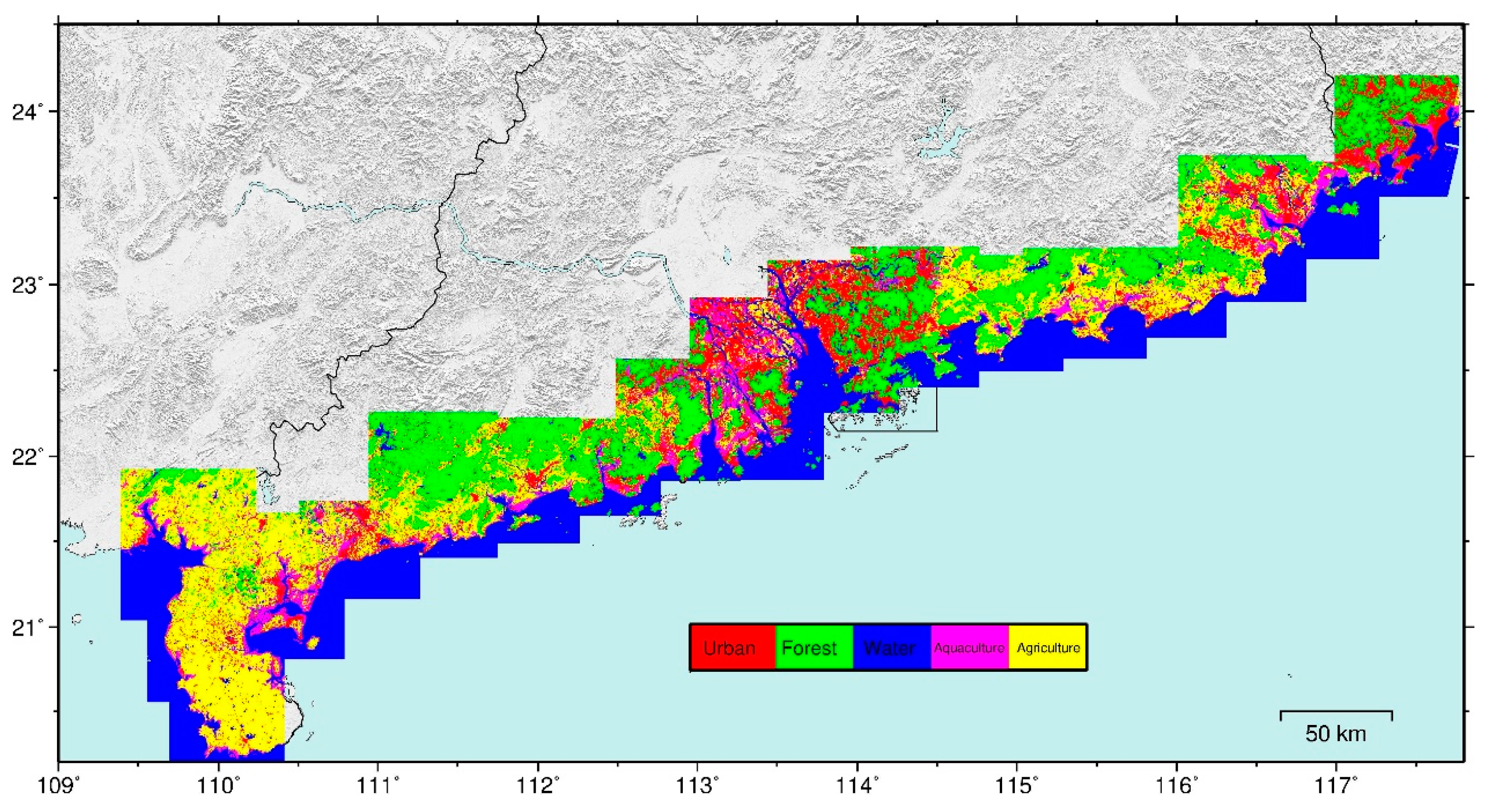
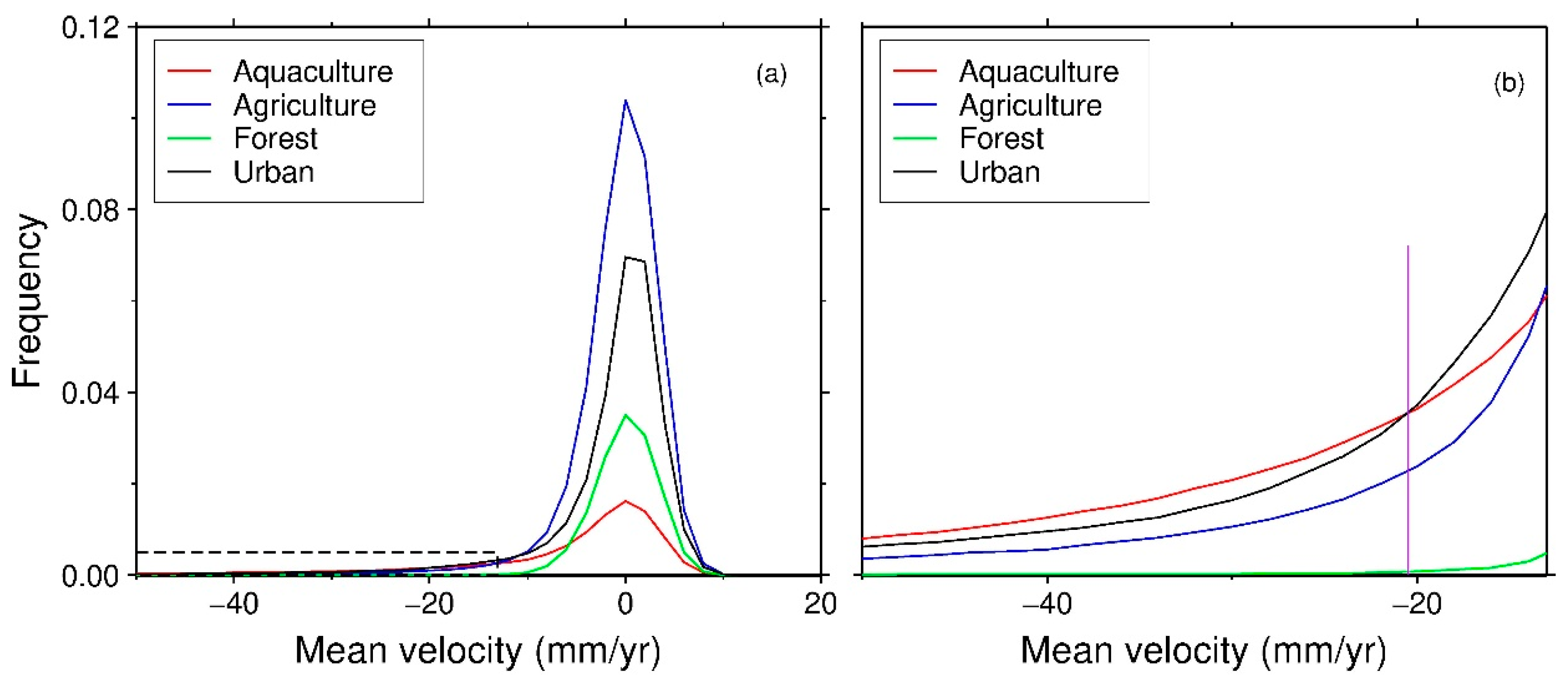
6.2. Quantitative Correlation between Subsidence and Land-Use Class

To analyze the correlation between subsidence and land-use class quantitatively, we generated a land-use classification map based on object-oriented segmentation, as shown in Figure 7. Four frequently used classes, agriculture, forest, urban, and water, marked by yellow, green, red, and blue shading are isolated. Notably, the urban land-use class includes manmade constructions, such as buildings and bridges, and bare soil due to their similarity in spectral information. In contrast to the previous classification results [28,33], the specific class of aquaculture is identified due to its wide range and its important role in the economy of Guangdong Province, as mentioned above. The aquaculture class is indicated by purple shading in Figure 7. The overall accuracy (OA) of the classification is about 89.5% with a land-use reference map derived from [49,50].

Comparing the subsidence map (Figure 3) with the classification map (Figure 7), we noticed that areas with notable subsidence rate (>20 mm/yr) are mainly aquaculture and agricultural areas, as indicated by purple and yellow shading in Figure 7, respectively. The representative subsidence areas in the aquaculture areas are in the LZP (Figure 8) and PRD (Figure 9). For example, the relevant optical images of the subsidence bowls in Leizhou Bay and Zhanjiang Bay and the other subsidence bowls along the coastline of the LZP are shown in the insets A–E of Figure 8. In the PRD, the majority of the subsidence (>20 mm/yr) is concentrated in aquaculture areas, the total area of which reaches 772.2 km². However, in the CSP, the subsidence is mainly located in the mixed area with agriculture and urban classes, see the yellow and red shading in Figure 7 for the two corresponding subsidence bowls, i.e., B1 and B2 in Figure 10. In addition to these representative areas, aquaculture areas along the coastline are also undergoing subsidence but exhibit different magnitudes of subsidence (see the insets A, B, and D in Figure 6). In addition to subsidence in aquaculture and agricultural areas, notable subsidence is also observed in forest and urban areas, for example, discrete subsidence bowls in forest areas of track 463 (inset C in Figure 6) and elongated subsidence in the Nansha district of Guangzhou (inset A in Figure 9a), petrochemical area of Daya Bay (inset E in Figure 6), and Macau airport (inset B in Figure 9a).

Although the correlation between subsidence and land use is obvious after qualitative comparison, to clarify this correlation, we also give the histograms of subsidence rate in four land-use classes, aquaculture, agriculture, forest and urban, as shown in Figure 12a. Notably, pixels in water areas are ignored because of low coherence. The highest subsidence (>20 mm/yr) is mainly focused in the aquaculture areas, followed by the subsidence in urban areas, agricultural areas, and finally forest (see the red, black, blue, and green lines in the insets of Figure 12b, respectively). The total percentages of the abovementioned subsidence in the four adopted classes are 40.8%, 37.1%, 21.5%, and 0.6%, respectively. Hence, aquaculture-induced groundwater exploitation is the major cause of the notable subsidence in Guangdong Province. Moreover, we also generated the percentage of different subsidence rate sections in each land-use class (see

Table 4. Percentage of subsidence velocity ranges within each land-use class.

Subsidence Rate (mm/yr)	Land-Use Class
	Aquaculture (%)	Agriculture (%)	Forest (%)	Urban (%)
(0, 5]	14.0	44.3	13.4	28.3
(5, 10]	26.3	34.5	6.3	32.9
(10, 20]	35.4	25.6	1.4	37.6
>20	40.8	21.5	0.6	37.1

). We can see that slow subsidence mainly occurs in agriculture areas, for example, 44.3% and 34.5% when the subsidence rate is within the range of (0, 5] and (5, 10], respectively.

6.3. Causes of Subsidence in Guangdong Province

The causes of surface subsidence are generally summarized as natural compression and artificial activities [26]. The latter is the main cause of surface subsidence in many coastal areas and deltas and includes fluid and solid resource exploitation, underground infrastructure construction and compaction of constructions overlaying the Holocene sediment. In Guangdong Province, both causes are involved and are thus qualitatively analyzed in the following points.

6.3.1. Subsidence Probably Caused by Groundwater Exploitation for Freshwater Aquaculture Use

The areas of subsidence rate > 20 mm/yr along the coastal area occur mainly in the aquaculture areas, as mentioned in Section 6.2. The aquaculture areas in the LZP and PRD account for 53.3% of the entire coastal area (see the purple shading in Figure 7). The corresponding subsidence areas in the LZP and PRD are 112.3 km² and 772.2 km², respectively. The maximum subsidence rates in these two areas are 58.0 mm/yr and 150.9 mm/yr, respectively. In addition to the subsidence bowls in the LZP and PRD, local subsidence bowls are also observed in the aquaculture area, see the insets B, D, and G in Figure 6. The water sources of these aquaculture areas are mainly derived from freshwater to satisfy the water quality required by the aquatic products, such as eel and tilapia [56,57]. Moreover, the frequency of freshwater exchange is high, aiming to improve the production and quality of the products. Hence, the very high requirement for freshwater and the obvious correlation between subsidence and aquaculture land use suggest that the exploitation of groundwater for aquaculture may be the primary cause of subsidence within these areas. However, we cannot analyze the explicit relationship between subsidence and groundwater exploitation volumes due to the vast illegal exploitation. Fortunately, deformation time series analysis is commonly adopted to analyze the subsidence caused by groundwater exploitation [26,28,29,58,59]. From the results in the aquaculture area (see Figure 8b,c and Figure 9b,c), the linear trend of the deformation time series is identified. This lack of seasonal variability is likely caused by the exploitation of groundwater from the confined aquifer instead of shallow aquifer, resulting in the phenomenon of continual subsidence.

6.3.2. Subsidence Probably Caused by Groundwater Exploitation for Agricultural and Residential Use

Subsidence caused by groundwater exploitation for agricultural and residential use is mainly located in the CSP and the inland area of the LZP [7,60]. Unlike the subsidence that occurs in the PRD, more concentrated subsidence at very high rates (maximum value of 157.2 mm/yr) and over large areas (342.2 km²) are observed in the mixed area of agricultural and residential land use (see B1 in Figure 10) in the CSP. Within the subsidence bowl, the percentages of manmade structures and agricultural lands are 58.6% and 30.3%, respectively, in addition to the small percentage (11.1%) of aquaculture land. Thus, groundwater exploitation for the mixture of residential and agricultural use may be the major cause of subsidence. Similarly, a linear time series instead of a seasonally variable time series is observed (see Figure 10b–e), indicating continued groundwater exploitation for residential use. In addition to the groundwater exploitation, the thick Quaternary deposits in the CSP (with a maximum thickness of 167 m) may accelerate the subsidence rate during groundwater exploitation. In addition, a wide range of slow subsidence is also observed in the agricultural land of the LZP. However, the deformation time series presents an obvious nonlinear characteristic (see Figure 8e), reflecting the seasonal irrigation in the LZP.

6.3.3. Subsidence Caused by Land Reclamation

In addition to the exploitation of groundwater, another dominant cause of surface subsidence is the compaction of the Q4 deposits under the overlying buildings or other infrastructures. These deposits possess a high pore ratio and low strength [61,62], resulting in subsidence due to the compaction of soft soil and aquifers. Moreover, the sea reclamation phenomenon in the PRD is widespread (see the areas between the blue and red lines in Figure 9), resulting in the accumulation and compaction of soft soil and finally leading to subsidence. For example, the deposit thickness map of the PRD in Figure 2 shows that the subsidence is mainly concentrated in the areas of soft soil, and the thicker the soft soil, the higher the subsidence rate is, as shown in Figure 11d.

6.3.4. Subsidence Caused by Other Reasons

In Zhanjiang and Shenzhen cities, elongated subsidence bowls with maximum subsidence rates of approximately 26.6 mm/yr and 51.4 mm/yr are observed, respectively. The bowls are located in urban areas with dense industries (see inset E in Figure 6 and the optical image in inset F of Figure 8), indicating groundwater exploitation for industrial use. Because groundwater needs for industry are high and persistent, a decline in groundwater level and continued subsidence are possible (see the corresponding deformation time series of industrial areas in Figure 8d). In addition, metro tunnel excavation is a cause of subsidence in urban areas, for example, the excavation of subway line 4 in the Nansha district of Guangzhou (see inset A in Figure).

In the LZP, discrete subsidence in a large agricultural area with a subsidence rate < 20 mm/yr is caused by not only groundwater exploitation but also natural compression, such as that due to the chemical erosion of peduncle [63].

In tracks 463 and 458, local subsidence bowls are found in forest areas and may be caused by slope instability (see insets C and F in Figure 6), potentially resulting in slow-moving landslides.

7. Conclusions

Through the use of two MTInSAR techniques, SBAS-InSAR and TCPInSAR, we obtained a large-scale deformation map for the coastal areas of Guangdong. We also identified three notable subsidence areas in LZP, PRD, and CSP, with maximum subsidence rates approximately 58 mm/yr, 150.9 mm/yr, and 157.2 mm/yr, respectively. The relative precision of the average subsidence velocity in the overlapped areas was generally below 3.2 mm/yr, except for several values ranging from 3.4 mm/yr to 4.3 mm/yr. The root-mean-square error (RMSE) of the velocity and deformation time series calculated between InSAR and GPS results are 1.8 mm/yr and 7.6 mm, respectively.

In addition to the subsidence map, a land-use map that identifies five classes (aquaculture, agricultural, urban, forest, and water) along the coastline was generated. The relationship between these two maps showed that a high subsidence rate (>20 mm/yr) mainly occurs in aquaculture areas, followed by urban agricultural and forest areas, accounting for 40.8%, 37.1%, 21.5%, and 0.6% of the total area with this notable subsidence rate, respectively. Subsidence due to land reclamation and manmade constructions was also monitored. Additionally, we also found that subsidence mainly occurs in the Holocene deposits, and a positive correlation between subsidence and Holocene deposit thickness is obtained after the interpolation of thickness from the selected borehole data. In addition to the average subsidence velocity, the linear deformation time series in the aquaculture and agricultural areas showed that the groundwater is probably exploited continuously, and the subsidence would continue along the coastal areas if no measures were adopted. The results highlight the aquaculture-induced subsidence, in addition to the more common agricultural-induced subsidence, along these coastal areas.

References

1. Marks, R. Robert Marks on the Pearl River Delta. Environ. Hist. 2004, 9, 296. [Google Scholar] [CrossRef]
2. Yeung, Y.-M. The further integration of the Pearl River Delta: A new beginning of reform. Environ. Urban. Asia 2010, 1, 13–26. [Google Scholar] [CrossRef]
3. Cao, L.; Wang, W.; Yang, Y.; Yang, C.; Yuan, Z.; Xiong, S.; Diana, J. Environmental impact of aquaculture and countermeasures to aquaculture pollution in China. Environ. Sci. Pollut. Res. 2007, 14, 452–462. [Google Scholar]
4. Du, Y.; Feng, G.; Peng, X.; Li, Z. Subsidence Evolution of the Leizhou Peninsula, China, Based on InSAR Observation from 1992 to 2010. Appl. Sci. 2017, 7, 466. [Google Scholar] [CrossRef] [Green Version]
5. Jiang, L.; Lin, H.; Cheng, S. Monitoring and assessing reclamation settlement in coastal areas with advanced InSAR techniques: Macao city (China) case study. Int. J. Remote Sens. 2011, 32, 3565–3588. [Google Scholar] [CrossRef]
6. Li, G. Analysis of regional subsidence of Zhanjiang city. West China Explor. Eng. 2009, 12, 108–110. [Google Scholar]
7. Liu, P.; Chen, X.; Li, Z.; Zhang, Z.; Xu, J.; Feng, W.; Wang, C.; Hu, Z.; Tu, W.; Li, H.J.R.S. Resolving surface displacements in Shenzhen of China from time series InSAR. Remote Sens. 2018, 10, 1162. [Google Scholar] [CrossRef] [Green Version]
8. Liu, Y.; Ma, P.; Lin, H.; Wang, W.; Shi, G. Distributed Scatterer InSAR Reveals Surface Motion of the Ancient Chaoshan Residence Cluster in the Lianjiang Plain, China. Remote Sens. 2019, 11, 166. [Google Scholar] [CrossRef]
9. Wang, H.; Feng, G.; Xu, B.; Yu, Y.; Li, Z.; Du, Y.; Zhu, J. Deriving spatio-temporal development of ground subsidence due to subway construction and operation in delta regions with PS-InSAR data: A case study in Guangzhou, China. Remote Sens. 2017, 9, 1004. [Google Scholar] [CrossRef] [Green Version]
10. Wang, H.; Wright, T.J.; Yu, Y.; Lin, H.; Jiang, L.; Li, C.; Qiu, G. InSAR reveals coastal subsidence in the Pearl River Delta, China. Geophys. J. Int. 2012, 191, 1119–1128. [Google Scholar] [CrossRef] [Green Version]
11. Zhao, Q.; Lin, H.; Jiang, L.; Chen, F.; Cheng, S. A study of ground deformation in the Guangzhou urban area with persistent scatterer interferometry. Sensors 2009, 9, 503–518. [Google Scholar] [CrossRef] [PubMed]
12. Bi, X.; Lu, Q.; Pan, X. Coastal use accelerated the regional sea-level rise. Ocean Coast. Manag. 2013, 82, 1–6. [Google Scholar] [CrossRef]
13. Poitevin, C.; Wöppelmann, G.; Raucoules, D.; Le Cozannet, G.; Marcos, M.; Testut, L. Vertical land motion and relative sea level changes along the coastline of Brest (France) from combined space-borne geodetic methods. Remote Sens. Environ. 2019, 222, 275–285. [Google Scholar] [CrossRef]
14. Wu, Q.; Zheng, X.; Xu, H.; Ying, Y.; Hou, Y.; Xie, X.; Wang, S. Relative sea-level rising and its control strategy in coastal regions of China in the 21st century. Sci. China 2003, 46, 2562–2571. [Google Scholar] [CrossRef]
15. Gattacceca, J.C.; Vallet-Coulomb, C.; Mayer, A.; Claude, C.; Radakovitch, O.; Conchetto, E.; Hamelin, B. Isotopic and geochemical characterization of salinization in the shallow aquifers of a reclaimed subsiding zone: The southern Venice Lagoon coastland. J. Hydrol. 2009, 378, 46–61. [Google Scholar] [CrossRef]
16. Berardino, P.; Fornaro, G.; Lanari, R.; Sansosti, E. A new algorithm for surface deformation monitoring based on small baseline differential SAR interferograms. IEEE Trans. Geosci. Remote Sens. 2002, 40, 2375–2383. [Google Scholar] [CrossRef] [Green Version]
17. Ferretti, A.; Prati, C.; Rocca, F. Nonlinear subsidence rate estimation using permanent scatterers in differential SAR interferometry. IEEE Trans. Geosci. Remote Sens. 2000, 38, 2202–2212. [Google Scholar] [CrossRef] [Green Version]
18. Zhang, Z.; Wang, C.; Zhang, H.; Tang, Y.; Liu, X. Analysis of permafrost region coherence variation in the Qinghai–Tibet Plateau with a high-resolution TerraSAR-X image. Remote Sens. 2018, 10, 298. [Google Scholar] [CrossRef] [Green Version]
19. Ferretti, A.; Fumagalli, A.; Novali, F.; Prati, C.; Rocca, F.; Rucci, A. A New Algorithm for Processing Interferometric Data-Stacks: SqueeSAR. IEEE Trans. Geosci. Remote Sens. 2011, 49, 3460–3470. [Google Scholar] [CrossRef]
20. Ferretti, A.; Prati, C.; Rocca, F. Permanent scatterers in SAR interferometry. IEEE Trans. Geosci. Remote Sens. 2001, 39, 8–20. [Google Scholar] [CrossRef]
21. Hooper, A.; Zebker, H.; Segall, P.; Kampes, B. A new method for measuring deformation on volcanoes and other natural terrains using InSAR persistent scatterers. Geophys. Res. Lett. 2004, 31. [Google Scholar] [CrossRef]
22. Zhang, L.; Ding, X.; Lu, Z. Modeling PSInSAR time series without phase unwrapping. IEEE Trans. Geosci. Remote Sens. 2011, 49, 547–556. [Google Scholar] [CrossRef]
23. Ao, M.; Wang, C.; Xie, R.; Zhang, X.; Hu, J.; Du, Y.; Li, Z.; Zhu, J.; Dai, W.; Kuang, C. Monitoring the land subsidence with persistent scatterer interferometry in Nansha District, Guangdong, China. Nat. Hazards 2015, 75, 2947–2964. [Google Scholar] [CrossRef]
24. Du, Y.; Feng, G.; Li, Z.; Peng, X.; Zhu, J.; Ren, Z. Effects of External Digital Elevation Model Inaccuracy on StaMPS-PS Processing: A Case Study in Shenzhen, China. Remote Sens. 2017, 9, 1115. [Google Scholar] [CrossRef] [Green Version]
25. Xu, B.; Feng, G.; Li, Z.; Wang, Q.; Wang, C.; Xie, R. Coastal subsidence monitoring associated with land reclamation using the point target based SBAS-INSAR method: A case study of shenzhen, China. Remote Sens. 2016, 8, 652. [Google Scholar] [CrossRef] [Green Version]
26. Abidin, H.Z.; Andreas, H.; Gumilar, I.; Fukuda, Y.; Pohan, Y.E.; Deguchi, T. Land subsidence of Jakarta (Indonesia) and its relation with urban development. Nat. Hazards 2011, 59, 1753. [Google Scholar] [CrossRef]
27. Chaussard, E.; Amelung, F.; Abidin, H.; Hong, S.-H. Sinking cities in Indonesia: ALOS PALSAR detects rapid subsidence due to groundwater and gas extraction. Remote Sens. Environ. 2013, 128, 150–161. [Google Scholar] [CrossRef]
28. Chaussard, E.; Wdowinski, S.; Cabral-Cano, E.; Amelung, F. Land subsidence in central Mexico detected by ALOS InSAR time-series. Remote Sens. Environ. 2014, 140, 94–106. [Google Scholar] [CrossRef]
29. López-Quiroz, P.; Doin, M.-P.; Tupin, F.; Briole, P.; Nicolas, J.-M. Time series analysis of Mexico City subsidence constrained by radar interferometry. J. Appl. Geophys. 2009, 69, 1–15. [Google Scholar] [CrossRef]
30. Erban, L.E.; Gorelick, S.M.; Zebker, H.A. Groundwater extraction, land subsidence, and sea-level rise in the Mekong Delta, Vietnam. Environ. Res. Lett. 2014, 9, 084010. [Google Scholar] [CrossRef]
31. Higgins, S.A. Review: Advances in delta-subsidence research using satellite methods. Hydrogeol. J. 2016, 24, 587–600. [Google Scholar] [CrossRef]
32. Mialhe, F.; Gunnell, Y.; Mering, C.; Gaillard, J.-C.; Coloma, J.G.; Dabbadie, L. The development of aquaculture on the northern coast of Manila Bay (Philippines): An analysis of long-term land-use changes and their causes. J. Land Use Sci. 2016, 11, 236–256. [Google Scholar] [CrossRef]
33. Huang, M.-H.; Bürgmann, R.; Hu, J.-C. Fifteen years of surface deformation in Western Taiwan: Insight from SAR interferometry. Tectonophysics 2016, 692, 252–264. [Google Scholar] [CrossRef] [Green Version]
34. Dong, H.; Huang, C.; Chen, W.; Zhang, H.; Zhi, B.; Zhao, X. The controlling factors of environment geology in the Pearl River Delta Economic Zone and an analysis of existing problems. Geol. China 2012, 39, 539–549. [Google Scholar]
35. Shen, J.H.; Wang, R.; Zhu, C.Q. Research on spatial distribution law of gray clays of Zhanjiang Formation. Rock Soil Mech. 2013, 34, 331–338. [Google Scholar]
36. Song, Y.S.; Chen, W.B.; Pan, H.; Zhang, Z.Z. Geological Age of Quaternary Series in Lianjiang Plain. J. Jilin Univ. (Earth Sci. Ed.) 2012, 42, 154–161. [Google Scholar]
37. Sun, J.L.; Hui-Long, X.U.; Peng, W.U.; Ye-Biao, W.U.; Qiu, X.L.; Zhan, W.H. Late Quaternary sedimentological characteristics and sedimentary environment evolution in sea area between Nan’ao and Chenghai, eastern Guangdong. J. Trop. Oceanogr. 2007, 26, 30–36. [Google Scholar]
38. Wang, J.H.; Zheng, Z.; Wu, C.Y. Sedimentary Facies and Paleoenvironmental Evolution of the Late Quaternary in the Chao Shan Plain, East Guangdong. Actaentiarum Nat. Univ. Sunyatseni 1997, 36, 95–100. [Google Scholar]
39. Zhou, X.; Chen, M.; Liang, C. Optimal schemes of groundwater exploitation for prevention of seawater intrusion in the Leizhou Peninsula in southern China. Environ. Geol. 2003, 43, 978–985. [Google Scholar] [CrossRef]
40. Statistical Bureau of Guangdong Province. Statistical Yearbook of Guangdong. Available online: http://stats.gd.gov.cn/gdtjnj/ (accessed on 17 November 2015).
41. Irons, J.R.; Dwyer, J.L.; Barsi, J.A. The next Landsat satellite: The Landsat data continuity mission. Remote Sens. Environ. 2012, 122, 11–21. [Google Scholar] [CrossRef] [Green Version]
42. Roy, D.P.; Wulder, M.A.; Loveland, T.R.; Woodcock, C.; Allen, R.G.; Anderson, M.C.; Helder, D.; Irons, J.R.; Johnson, D.M.; Kennedy, R. Landsat-8: Science and product vision for terrestrial global change research. Remote Sens. Environ. 2014, 145, 154–172. [Google Scholar] [CrossRef] [Green Version]
43. Zhang, Y.; Wu, H.; Kang, Y.; Zhu, C. Ground subsidence in the Beijing-Tianjin-Hebei region from 1992 to 2014 revealed by multiple sar stacks. Remote Sens. 2016, 8, 675. [Google Scholar] [CrossRef] [Green Version]
44. Samsonov, S. Topographic correction for ALOS PALSAR interferometry. IEEE Trans. Geosci. Remote Sens. 2010, 48, 3020–3027. [Google Scholar] [CrossRef]
45. Zhang, L.; Lu, Z.; Ding, X.; Jung, H.-S.; Feng, G.; Lee, C.-W. Mapping ground surface deformation using temporarily coherent point SAR interferometry: Application to Los Angeles Basin. Remote Sens. Environ. 2012, 117, 429–439. [Google Scholar] [CrossRef]
46. Zhang, L.; Ding, X.; Lu, Z.; Jung, H.-S.; Hu, J.; Feng, G. A novel multitemporal InSAR model for joint estimation of deformation rates and orbital errors. IEEE Trans. Geosci. Remote Sens. 2014, 52, 3529–3540. [Google Scholar] [CrossRef] [Green Version]
47. Xu, Q. A ground crack longitudinally penetrating the holocene sand dyke in Gangzi, Leizhou Peninsula is discovered. Quat. Sci. 2008, 28, 712–720. [Google Scholar]
48. Blaschke, T. Object based image analysis for remote sensing. ISPRS J. Photogramm. Remote Sens. 2010, 65, 2–16. [Google Scholar] [CrossRef] [Green Version]
49. Li, C.; Gong, P.; Wang, J.; Zhu, Z.; Biging, G.S.; Yuan, C.; Hu, T.; Zhang, H.; Wang, Q.; Li, X. The first all-season sample set for mapping global land cover with Landsat-8 data. Sci. Bull. 2017, 62, 508–515. [Google Scholar] [CrossRef] [Green Version]
50. National Earth System Science Data Center. National Science & Technology Infrastructure of China. Available online: http://www.geodata.cn (accessed on 1 February 2018).
51. Casu, F.; Manzo, M.; Lanari, R. A quantitative assessment of the SBAS algorithm performance for surface deformation retrieval from DInSAR data. Remote Sens. Environ. 2006, 102, 195–210. [Google Scholar] [CrossRef]
52. Costantini, M.; Ferretti, A.; Minati, F.; Falco, S.; Trillo, F.; Colombo, D.; Novali, F.; Malvarosa, F.; Mammone, C.; Vecchioli, F. Analysis of surface deformations over the whole Italian territory by interferometric processing of ERS, Envisat and COSMO-SkyMed radar data. Remote Sens. Environ. 2017, 202, 250–275. [Google Scholar] [CrossRef]
53. Zhao, C.; Liu, C.; Zhang, Q.; Lu, Z.; Yang, C. Deformation of Linfen-Yuncheng Basin (China) and its mechanisms revealed by Π-RATE InSAR technique. Remote Sens. Environ. 2018, 218, 221–230. [Google Scholar] [CrossRef]
54. Bagliani, A.; Mosconi, A.; Marzorati, D.; Cremonesi, A.; Ferretti, A.; Colombo, D.; Novali, F.; Tamburini, A. Use of satellite radar data for surface deformation monitoring: A wrap-up after 10 years of experimentation. In Proceedings of the SPE Annual Technical Conference and Exhibition, Florence, Italy, 20–22 September 2010. [Google Scholar]
55. Bonì, R.; Herrera, G.; Meisina, C.; Notti, D.; Béjar-Pizarro, M.; Zucca, F.; González, P.J.; Palano, M.; Tomás, R.; Fernández, J. Twenty-year advanced DInSAR analysis of severe land subsidence: The Alto Guadalentín Basin (Spain) case study. Eng. Geol. 2015, 198, 40–52. [Google Scholar] [CrossRef] [Green Version]
56. FAO. National Aquaculture Sector Overview. China. In National Aquaculture Sector Overview Fact Sheets; FAO: Rome, Italy, 2005. [Google Scholar]
57. Gu, D.E.; Yu, F.D.; Yang, Y.X.; Xu, M.; Wei, H.; Luo, D.; Mu, X.D.; Hu, Y.C. Tilapia fisheries in Guangdong Province, China: Socio-economic benefits, and threats on native ecosystems and economics. Fish. Manag. Ecol. 2019, 26, 97–107. [Google Scholar] [CrossRef]
58. Bell, J.W.; Amelung, F.; Ferretti, A.; Bianchi, M.; Novali, F. Permanent scatterer InSAR reveals seasonal and long-term aquifer-system response to groundwater pumping and artificial recharge. Water Resour. Res. 2008, 44, 282–288. [Google Scholar] [CrossRef] [Green Version]
59. Van der Horst, T.; Rutten, M.M.; van de Giesen, N.C.; Hanssen, R.F. Monitoring land subsidence in Yangon, Myanmar using Sentinel-1 persistent scatterer interferometry and assessment of driving mechanisms. Remote Sens. Environ. 2018, 217, 101–110. [Google Scholar] [CrossRef] [Green Version]
60. Jing, L. Environmental and geological problems caused by over-exploitation of groundwater and its prevention of Guangdong Province. Chin. J. Geol. Hazard Control 2007, 18, 64–67. [Google Scholar]
61. Carrera-Hernández, J.; Gaskin, S. The Basin of Mexico aquifer system: Regional groundwater level dynamics and database development. Hydrogeol. J. 2007, 15, 1577–1590. [Google Scholar] [CrossRef]
62. Terzaghi, K. Erdbaumechanik auf Bodenphysikalischer Grundlage; Franz Deuticke: Wien, Austria, 1925. [Google Scholar]
63. Galloway, J.N.; Townsend, A.R.; Erisman, J.W.; Bekunda, M.; Cai, Z.; Freney, J.R.; Martinelli, L.A.; Seitzinger, S.P.; Sutton, M.A. Transformation of the nitrogen cycle: Recent trends, questions, and potential solutions. Science 2008, 320, 889–892. [Google Scholar] [CrossRef] [Green Version]
Figure 1. Data coverage and geology formation along the coastline of Guangdong Province. (a) Blue solid and red dotted rectangles represent the collected synthetic aperture radar (SAR) images and Landsat optical images, respectively. The black stars represent the GPS stations used, and the gray lines represent faults. (b) The location of the study area.
Remotesensing 12 00299 g001
Figure 2. Sedimentary thickness map of the Leizhou Peninsula (LZP), Pearl River Delta (PRD) and Chanshao Plain (CSP). The cyan filled lines represent the primary rivers along the coastline. The black hollow circles represent the locations of the sediment depth measurements collected from boreholes. The purple circles represent the city along the coastal areas of Guangdong Province.
Remotesensing 12 00299 g002
Figure 3. Flowchart of data processing.
Remotesensing 12 00299 g003
Figure 4. Accuracy of InSAR-derived results. (a) The average deformation rate difference in the overlapping areas of adjacent tracks. Blue bars represent the histograms of the average rate difference, and black lines represent the normal distribution fitting of these rate differences; (b) The average deformation rate difference between the InSAR results and the GPS station results.
Remotesensing 12 00299 g004
Figure 5. Deformation time series comparison between InSAR and GPS results. Blue dots represent the GPS time series, and red triangles represent the InSAR time series.
Remotesensing 12 00299 g005
Figure 6. Average surface deformation map along the coastline of Guangdong. Yellow and purple shading represent surface motion toward and away from the satellite, respectively. Seven insets with obvious deformation rates are selected: (A) Hailing Bay, (B) the estuary of the Moyang River, (C,F) forest areas in tracks 463 and 457, respectively, (D) the estuary of Guanghai Bay, (E) the petrochemical area of Daya Bay, and (G) the estuary of the Haungjiang River.
Remotesensing 12 00299 g006
Figure 7. Land-use classification map. The red, green, blue, purple and yellow shading represent urban, forest, water, aquaculture and agricultural land uses.
Remotesensing 12 00299 g007
Figure 8. (a) Average surface deformation map of Leizhou Peninsula (LZP). Black solid circles are the selected subsidence bowls. Insets (A) to (F) are the corresponding optical images of the selected subsidence bowls. The black dotted circle represents the primary subsidence areas with a notable subsidence rate. P1 and P2 are two selected points located in aquaculture lands, P3 located in urban land, and P4 located in agricultural land. (be) are the corresponding time series of the four selected points.
Remotesensing 12 00299 g008
Figure 9. Average surface deformation map of the Pearl River Delta (PRD). Black solid circles B1 and B2 are two primary subsidence bowls with obvious deformation rates. Blue and red lines represent the coastlines in 1984 and 2011, respectively. Black stars represent the selected GPS stations. Purple dotted circles indicate the two selected districts, Jinwan (J.W.D) and Nansha (N.S.D). Black dotted circles represent the remaining topography-related atmospheric effects. Insets (a,b) are two selected urban areas. P1 and P2 are two selected points located in aquaculture lands, P3 and P4 are two points located in agricultural lands. (be) show the corresponding time series of the four selected points. (fi) are the corresponding optical images for the four points.
Remotesensing 12 00299 g009
Figure 10. (a) Average surface deformation map of the Chaoshan Plain (CSP). Black solid circles B1 and B2 are two primary subsidence bowls with notable deformation rates. Purple, black and red dotted circles represent the Lianjiang Plain, Rongjiang Plain, and Hanjiang Plain, respectively. Cyan filled lines in the inset indicate the three primary rivers, the Lianjiang River (L.J.), Rongjiang River (R.J.) and Hanjiang River (H.J.). P1 to P4 are four selected points located in the mixed agricultural and urban land areas. (be) are the corresponding time series of the four selected points. (fi) are the corresponding optical images for the four points.
Remotesensing 12 00299 g010
Figure 11. A quantitative relationship between subsidence and sedimentary thickness. (a) Deformation velocity histogram within (blue bars) and without (red bars) Holocene (Q4) deposits. (bd) Histograms of sedimentary thicknesses in the LZP, CSP, and PRD. White bars represent the pixel numbers in the thickness bins, and red diamonds represent the average deformation velocity in the thickness bins.
Remotesensing 12 00299 g011
Figure 12. Average deformation velocity in the four selected land-use classes. (b) The enlarged view of the black dotted rectangles in (a). Red, blue, green and black lines represent the histograms for aquaculture, agriculture, forest, and urban areas, respectively. The horizontal axis represents the average deformation velocity. The vertical axis represents the average velocity frequency in the four land-use classes.
Remotesensing 12 00299 g012