A Covariance-Based Approach to Merging InSAR and GNSS Displacement Rate Measurements

Remote Sensing Technology Institute German Aerospace Center (DLR) Münchenerstraße 20, 82234 Weßling, Germany
*
Author to whom correspondence should be addressed.
Remote Sens. 2020, 12(2), 300; https://0-doi-org.brum.beds.ac.uk/10.3390/rs12020300
Submission received: 4 December 2019
/
Revised: 1 January 2020
/
Accepted: 2 January 2020
/
Published: 16 January 2020
(This article belongs to the Special Issue Ground Deformation Patterns Detection by InSAR and GNSS Techniques)
Abstract
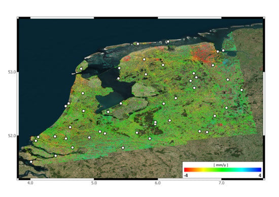
:This paper deals with the integration of deformation rates derived from Synthetic Aperture Radar Interferometry (InSAR) and Global Navigation Satellite System (GNSS) data. The proposed approach relies on knowledge of the variance/covariance of both InSAR and GNSS measurements so that they may be combined accounting for the spectral properties of their errors, hence preserving all spatial frequencies of the deformation detected by the two techniques. The variance/covariance description of the output product is also provided. A performance analysis is carried out on realistic simulated scenarios in order to show the boundaries of the technique. The proposed approach is finally applied to real data. Five Sentinel-1A/B stacks acquired over two different areas of interest are processed and discussed. The first example is a merged deformation map of the northern part of the Netherlands for both ascending and descending geometries. The second example shows the deformation at the junction between the North and East Anatolian Fault using three consecutive descending stacks.
1. Introduction and Motivation
Synthetic Aperture Radar Interferometry (InSAR) deformation rate measurements support a wide range of applications in the fields of geology, geophysics, and geohazards [1]. Since the nature of the interferometric measurements is inherently relative, the additive delays—like those of the troposphere and ionosphere—make the accuracy of such measurements strongly dependent on the distance [2,3,4]. Hence, InSAR performance varies according to the particular application. Typically, interferometry works well for applications such as infrastructure monitoring or urban subsidence, since they involve relatively short scales (10–20 km). However, there is also scientific interest in using InSAR to measure the strain accumulation of tectonic faults. This type of study requires very accurate measurements (1 mm/year at distances larger than 100 km) [5].
The new generation of Synthetic Aperture Radar (SAR) sensors—like Sentinel-1—provides systematically acquired data with a swath width of 250 km [6]; future missions plan to further extend this to 350 km [7]. Due to the atmospheric errors at such scales, the requirement of 1 mm/y could be a challenging goal for InSAR, especially if the available time series have a reduced observation time [8]. Therefore, in order to fully exploit the coverage capabilities of these missions, we are motivated to develop techniques that merge interferometric deformation rates with other geodetic measurements, not only to improve the performance of applications particularly affected by atmospheric effects (e.g., inter-seismic deformations), but also to remove the reference point, hence facilitating an easier integration with the other geometries or techniques.
The best candidate for this integration with SAR interferometry are the deformation rates estimated using a Global Navigation Satellite System (GNSS). This is due firstly to their well-known complementarity where InSAR coverage is combined with GNSS accuracy. Indeed, there is a long tradition of research in this area as evidenced by studies performed by geo-scientists; for example, in supporting interferometric phase unwrapping [9,10]. Combining InSAR and GNSS deformation rates has also been studied in order to calibrate the InSAR-estimated velocities [11,12,13], and to help the limited geometric sensitivity of the SAR system in measuring deformation [14,15,16]. The integration of InSAR with other instrumentation such as active transponders has been investigated in order to design optimal geodetic networks that enhance the spatial distribution of the deformation measurements [17,18,19].
However, it is important to highlight that the main argument of this work is not to claim the complementary InSAR/GNSS—which is well known, as previously mentioned—but rather to discuss the use of their error statistics in the combination, as well as its propagation through to the final product. In [8], the effect of the correction of the interferometric phase for tropospheric delays and solid earth tides using external models was shown. After such corrections, the mean variograms of the interferometric measurements error show a stationary behavior that can be well approximated by a covariance function. An optimal combination of the two measurement techniques is hence possible, since the spectral properties of their own errors can be taken into account. Moreover, no assumptions about the displacement pattern characteristics [19] and GNSS measurement density are necessary as in [11] and the data need not be filtered. Only the InSAR/GNSS differences, which can be statistically characterized, are estimated and used to compensate the original InSAR measurements. The error can then be propagated from the data to the results, allowing full characterization of the output uncertainty.
The measurement of strain accumulation along hundreds of kilometers is a potential application for this framework. The integration of InSAR and GNSS does not remove any deformation component, but performs a weighted merging of the different spatial frequencies of the deformation detected by the two techniques according to their reliability. Moreover, the mathematical modeling, often applied on final measurements, requires a proper weighting of the different input data [20]. Other possible applications include the InSAR-based National Ground Motion Services [21]. Such projects are often required to provide a product that merges the InSAR-derived results and the results derived by the GNSS networks already deployed on the territory. Since these products are part of a Service, a consistent description and traceability of the uncertainties is strictly required.
In Section 2 the proposed methodology is described, separating the capability of retrieving the absolute motion from the calibration of the residual atmospheric errors. An analytical description of the error of the merged product is also provided. In Section 3, simulations are performed in order to provide reference numbers in terms of coverage and quality versus performance. Finally, the results of using real data in significant test cases are presented and discussed. The first example covers the northern part of the Netherlands and demonstrates merging on a large scale in order to provide a consistent product like those in national ground motion services. The second example is aimed at addressing geophysical applications, and shows the calibration of interferometric measurements over North Anatolian Fault to the Eurasian plate.
2. Methodology
Let us consider N locations in the processed area of interest, where two deformation rate measurements and are performed using InSAR and GNSS, respectively. With as the radar line of sight (LoS) it is possible to state the problem modeling the difference between the two velocities at the ith position as follows:
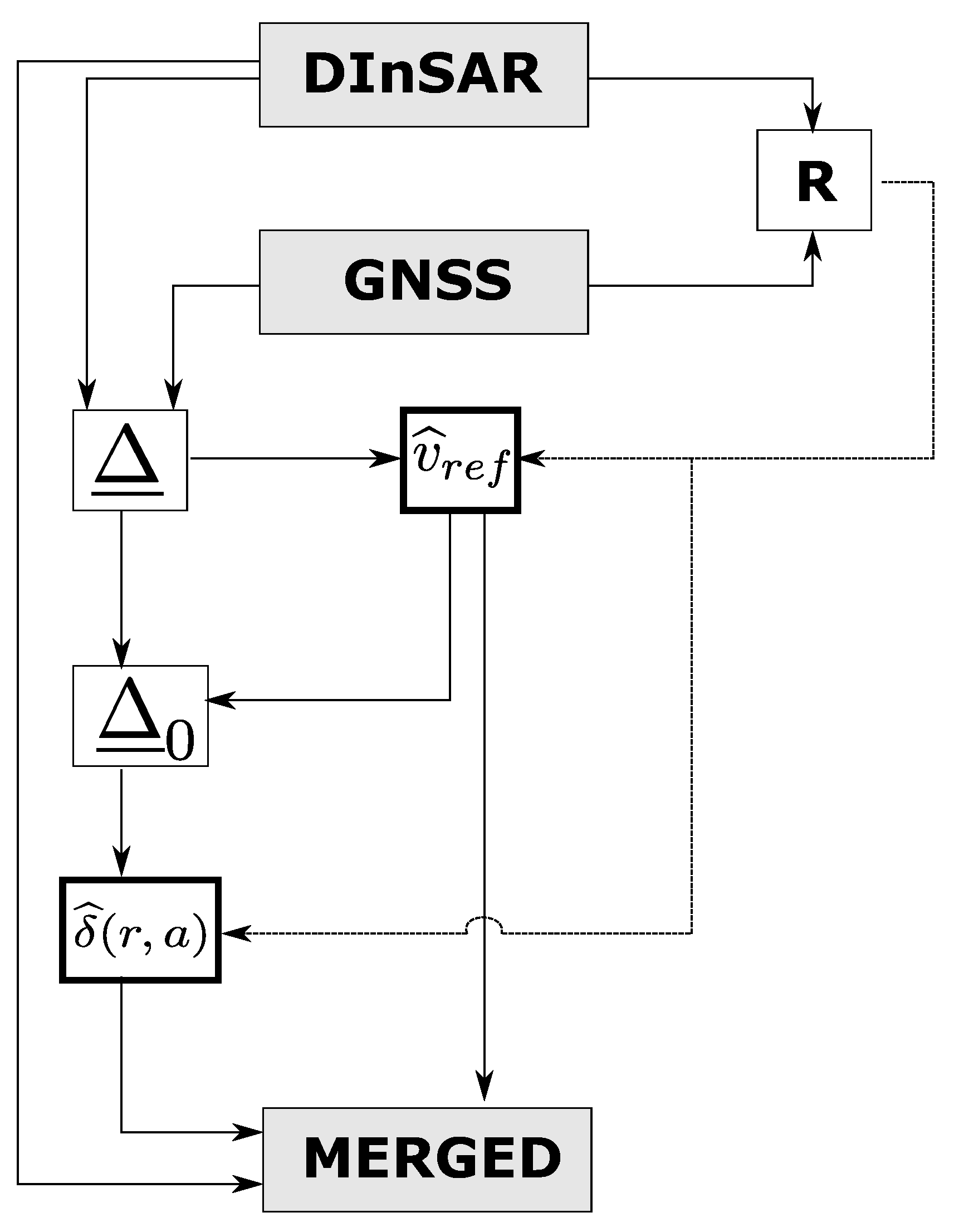
where is the velocity of the reference point used in InSAR processing, is a space-variant error screen in the interferometric data, and is the random error. The implicit hypothesis behind this definition is that the spatially correlated noise, basically related to the residual atmospheric delay, is present in the interferometric measurement only. This characteristic allows extraction, through the subtraction of the two velocities, of the parameters and , which have to be estimated in order to properly merge the data. It is worth noticing that this operation can also be seen as a calibration of the InSAR data: It exploits GNSS reference rates so that the interferometric measurement is no longer relative to the reference point while also removing residual systematic effects. Figure 1 displays an overview of the steps of the proposed approach. In the first step, the error statistics are derived and the covariance matrix is computed. The reference point velocity is then estimated and subtracted from the offset vector . Finally, the residual error screen is interpolated at each InSAR measurement point, exploiting knowledge of the error statistics.
2.1. Error Description of the Input Data
A proper handling of the relation defined in Equation (1) requires a statistical description of the vector . Therefore, the covariance matrix of the difference measurements has to be derived. It is possible to distinguish between three contributions: The random noise of the GNSS measurements obtained by projecting the variance of the different components of the estimated rates onto the radar LoS, the random noise of the InSAR measurements , and spatially correlated noise due to residual atmospheric effects. The full covariance matrix can be defined as:
The first two contributions are diagonal matrices, since they represent the spatially uncorrelated errors of the independent GNSS and InSAR measurement processes, respectively. On the other hand, the derivation of the covariance matrix that represents the residual atmospheric error is particularly interesting [22]. A covariance function representing the residual error has to be robustly estimated and evaluated at the N positions where the are located; with as the distance between the ith and the jth measurement, this is:
The first two components of Equation (2) can be estimated using the supplied accuracy of the GNSS data and the interferometric temporal coherences, respectively. However, estimation of requires a more detailed discussion.
2.2. Estimation of the Residual Atmospheric Error Covariance Matrix
The covariance of the residual atmospheric error can be estimated from interferograms where the residual atmospheric delay is the dominant measured delay. The fast revisit time of the Sentinel-1 mission allows the computation of short time interferograms with temporal baselines down to 6 days. Following the approach in [8], the short temporal baseline interferograms are used to compute variograms merely representing the residual atmospheric errors. Since such errors are expected to be on the order of magnitude of a centimeter, deformation rates of several tens of cm/y are necessary in order to bias the estimation of atmospheric errors. Such rates can be reached in landslides or mining areas that are typically restricted in coverage. Since the variograms are computed by averaging many different measurements over the whole scene, the effect of such areas should not strongly impact the estimation. It should be noted that since variogram estimation requires the unwrapped phase, this step must be performed at the end of the processing. At this stage, areas of very high deformation are apparent and can eventually be masked out. The effect of solid earth tides has been corrected in the interferometric phase using models [8]. However, the projection of tectonic plate motion onto the line of sight is a large-scale effect whose spatial characteristics cause a bias in variogram estimation. Such movements are mainly horizontal and can reach 6–7 cm/y. How large the horizontal motion must be in order to be comparable with the troposphere in a short temporal baseline interferogram can be easily estimated. For a 1 cm gradient along the radar swath, a horizontal motion of is necessary where is the incidence angle at near range and the incidence angle at far range, leading to a horizontal motion of cm or 152 cm/y for a revisit time of 12 days. Therefore, keeping the maximum days should result in negligible impact. It should be mentioned that the eventual presence of seismic events in the time series should also be assessed, and co-seismic interferometric pairs not be used to generate the variograms.
Given that such interferograms are almost deformation-free, it is possible to assume that the average of the variograms is a good estimator (the symbol indicates an estimated parameter) of the covariance characteristics of the residual atmospheric delays. Since velocity estimation implies a linear regression on the phase, a scaling factor accounting for acquisitions’ time span and number must be applied to convert the single-phase measurement accuracy into deformation rate accuracy:
where d is the distance, the radar wavelength, the acquisition times, and M the number of interferograms used for the linear regression. The analysis in [8] showed that if atmospheric phase corrections based on European Centre for Medium-Range Weather Forecasts (ECMWF) models are performed [23,24], the residual atmospheric effects after processing are well-modeled as stationary.
2.3. Estimation of the Reference Point Motion
Equation (1) shows how can be seen as an observation of with superimposed random and colored noise. Since the noise statistics of exhibit stationary behavior, the derivation of the reference point velocity can be carried out by averaging the observed . Therefore, according to the considerations in the previous Section 2.1, can be found by taking into account the computed covariance matrix :
where is a unitary vector that maps, one to one, the measurements with the unknown scalar . The estimated represents the motion of the reference point in its local LoS and has to be added to the InSAR velocities in order to make them absolute.
2.4. Estimation of the 0-Mean Calibration Screen
In the previous Section 2.3, the overall offset between InSAR and GNSS deformation rates was estimated while accounting for the covariance matrix. Now, the space-variant error screen between the GNSS and InSAR velocities can be estimated by performing a covariance-based interpolation (Kriging) of the residual offsets . A set of coefficients that, combined with the vector , allows the reconstruction of everywhere must be estimated.
According to theory, this can be obtained by imposing the condition that the interpolation/prediction error be uncorrelated:
with the data [25]. Substituting Equation (6) into Equation (7) and imposing the uncorrelatedness condition with gives:
where is the vector representing the correlation between the data vector and the error screen at the current position.
2.5. Variance and Covariance of the Results
To enhance usability, the error of the final product should be characterized. The final result is obtained by compensating the InSAR velocities for the estimated and . The reference point deformation rate is a bias added to all points. Its error is therefore a constant value in the final product. Its contribution can be derived by computing the variance of the linear system inversion:
The error of the estimated will be space variant. The variance and covariance of the estimated error screen can be derived as in [25].
where represents the original error due to the spatially correlated signal, and the second part of the equation represents a “mitigation factor” that reduces such variance according to the distance from the GNSS data. Analogously, the covariance is:
Some conclusions concerning the final product can now be drawn. It provides absolute measurements that can be characterized by a variance directly derived from the applied methodology. It still contains a residual spatial correlation, though mitigated by the removal of . However, this residual error is no longer stationary. Its covariance depends on the two considered points, as highlighted by Equation (11). The variogram or covariance representation of the error—as for the input InSAR velocities—is hence no longer possible, but must must to be computed locally, accounting for the position with respect to the GNSS stations.
3. Simulations
Simulations were performed in order to assess the validity of the method and evaluate its performance. The scope of these simulations is to understand and quantify the effects of the spatial distribution (density) and the quality of the GNSS measurements in different processing scenarios, and to provide some numbers that summarize the achievable accuracies in the retrieval of and .
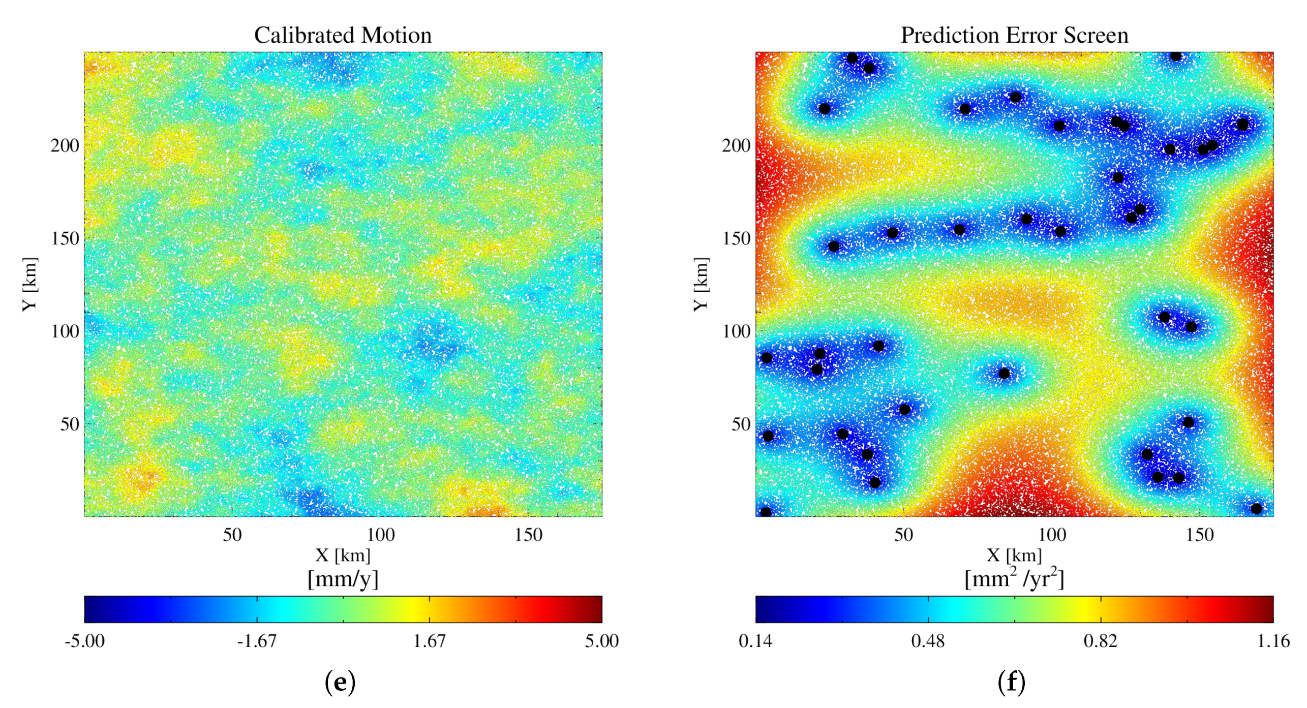
A set of randomly distributed points with zero deformation was simulated over a surface of km (Sentinel-1 slice size) in order to represent the InSAR measurements. Random noise (clutter) and spatially correlated noise (atmospheric residuals) were added to the points. For the generation of spatially correlated noise, an exponential covariance was used. A reduced set of GNSS zero-deformation data were also simulated at random positions within the scene. According to the model only random noise was added to the simulated GNSS velocities. For the sake of simplicity, positions were uniformly distributed within the scene. The reconstruction depends on how well the available samples are able to represent the error spectrum. In practice, the more high-pass the error, the more samples will be needed. Of course, a regular sampling is desirable. If the data are concentrated in an area, the re-construction will be good in this area. When moving away from data points, the estimator will extrapolate.
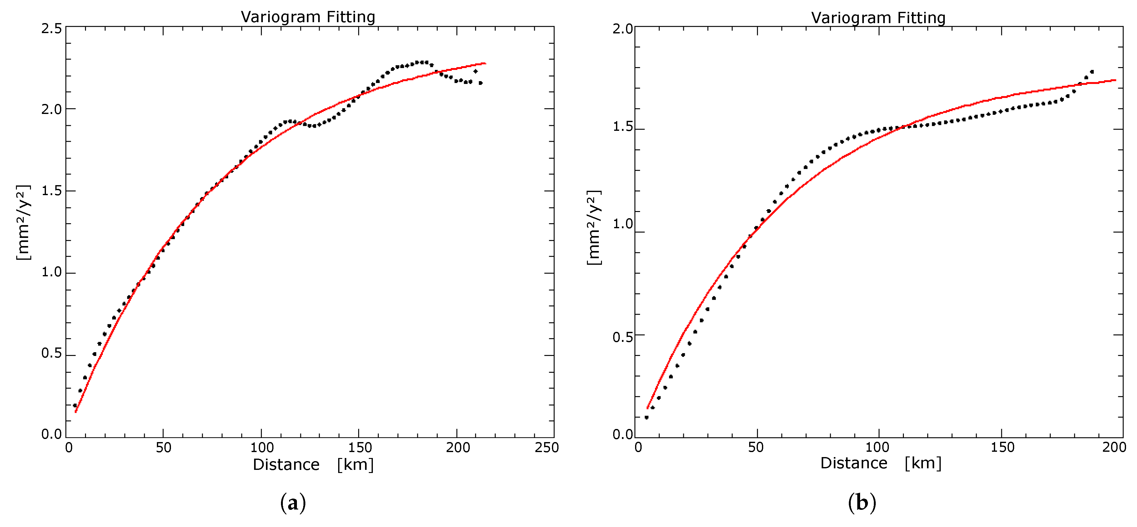
The simulations were performed while varying the two main parameters, the number of reference GNSS measurements, and their accuracy. Two different scenarios were tested with low and high atmospheric residual power . In the first scenario, ; for the Sentinel-1 mission, this is comparable to having a long time series of y in the case of applied atmospheric corrections [8]. In the second scenario, , representing the case of a short time series of y [8]. A realistic correlation length, according to real data, was used for the simulations— km in both cases. This comes from direct experience with the data. We observed that the average variograms after tropospheric corrections exhibited values of 40–100 km when fitted with an exponential model. An example of the simulation framework is shown in Figure 3.
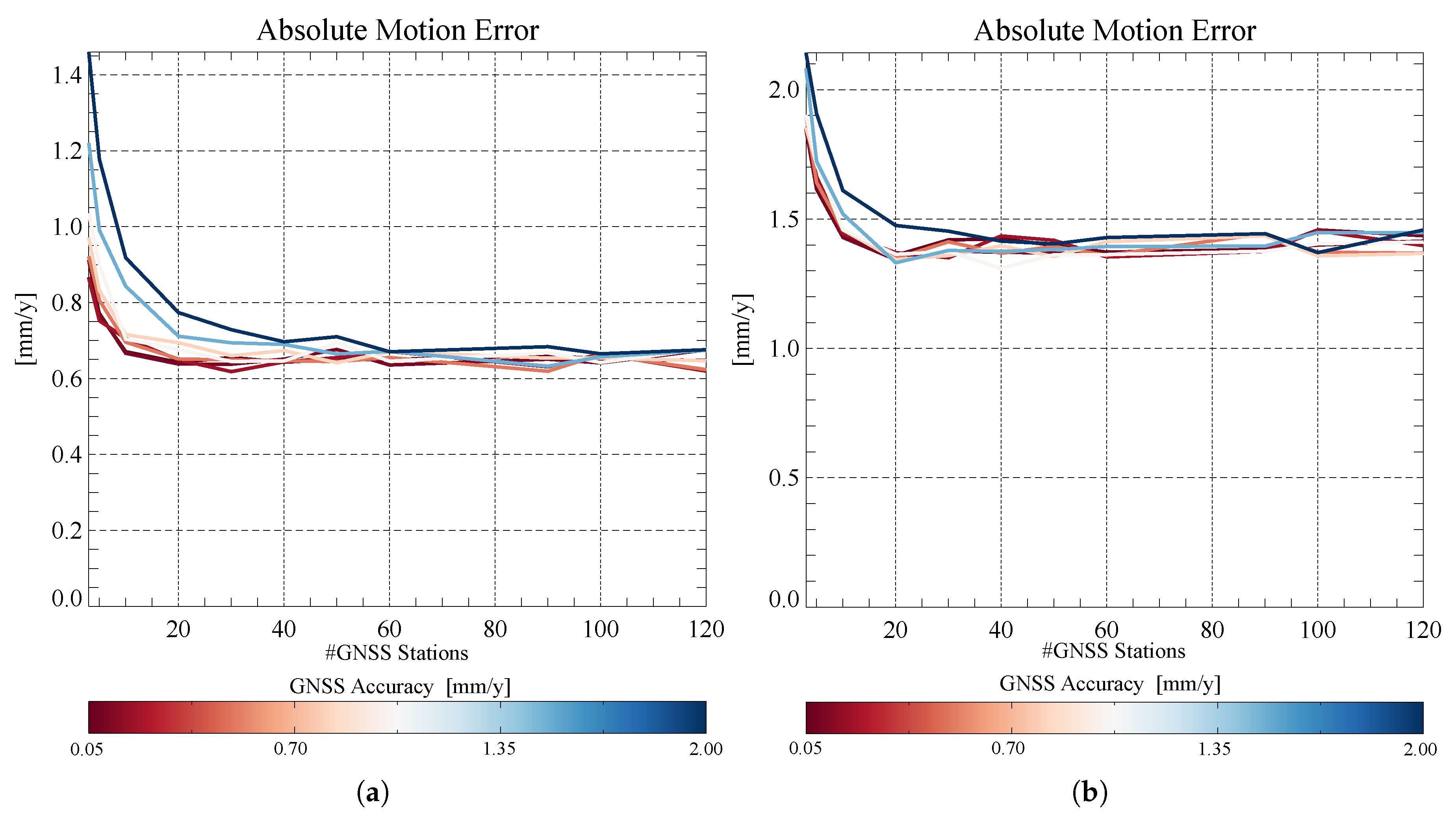
Observing the simulation results in Figure 4 and Figure 5 it can be concluded that, due to the spatial correlation of the error, higher densities of GNSS measurements improves the estimation of since it provides a better sampling of the error field, but does not help much in retrieving the absolute velocity , due to the “data redundancy” introduced by the spatial covariance.
3.1. Performance in Retrieving
The accuracy of is that of the mean computed from a set of correlated samples. The level of dependence of the given dataset is controlled by the spatial density of the latter and the correlation length of the superimposed noise. We observed that it is logical to expect that, given a , increasing the number of data improves estimation of up to a certain level, since as the density of measurements increases, so to does the amount of correlation between measurement, hence limiting its impact on final performance. In a typical scenario ( 3 y, 2 mm/y), the accuracy can easily be brought below 1 mm/y, even with a limited set of GNSS stations (Figure 4).
3.2. Performance in Retrieving
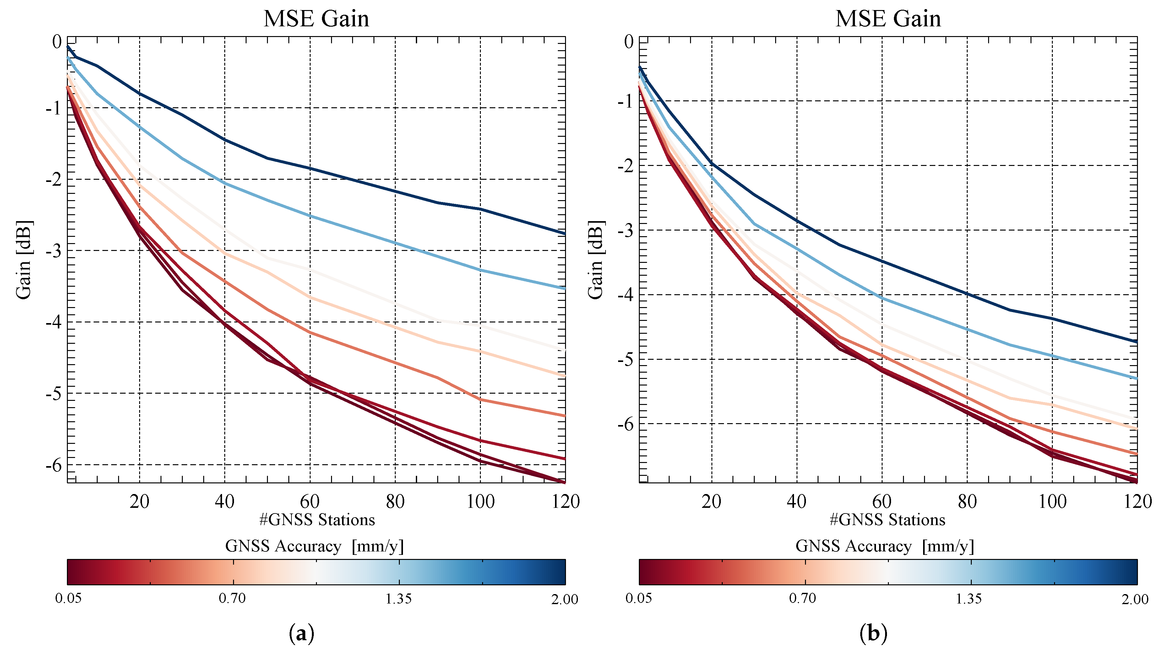
Evaluating the performance of is not a simple task. The most natural way would be to compare the variograms of the results before and after application of the technique. This approach would deliver a deeper insight into the achieved gain, since it would be possible to show this as a function of the scale. However, as mentioned in Section 2.5, the error of the merged results is no longer stationary making a variogram representation questionable. In order to avoid this issue, a simpler but more robust approach was followed. The performances were evaluated in terms of mean square error (MSE) in , over the whole scene. In practice, the mean power of the residual deformation signal after removal of the estimated error screen from the measured rates is:
The results displayed in Figure 5a,b show that, in both cases, the performance cannot improve beyond a certain level by improving the quality of the GNSS measurements only. An improvement in GNSS coverage is also necessary in order to better compensate the higher wave-numbers of the error screen.
4. Results
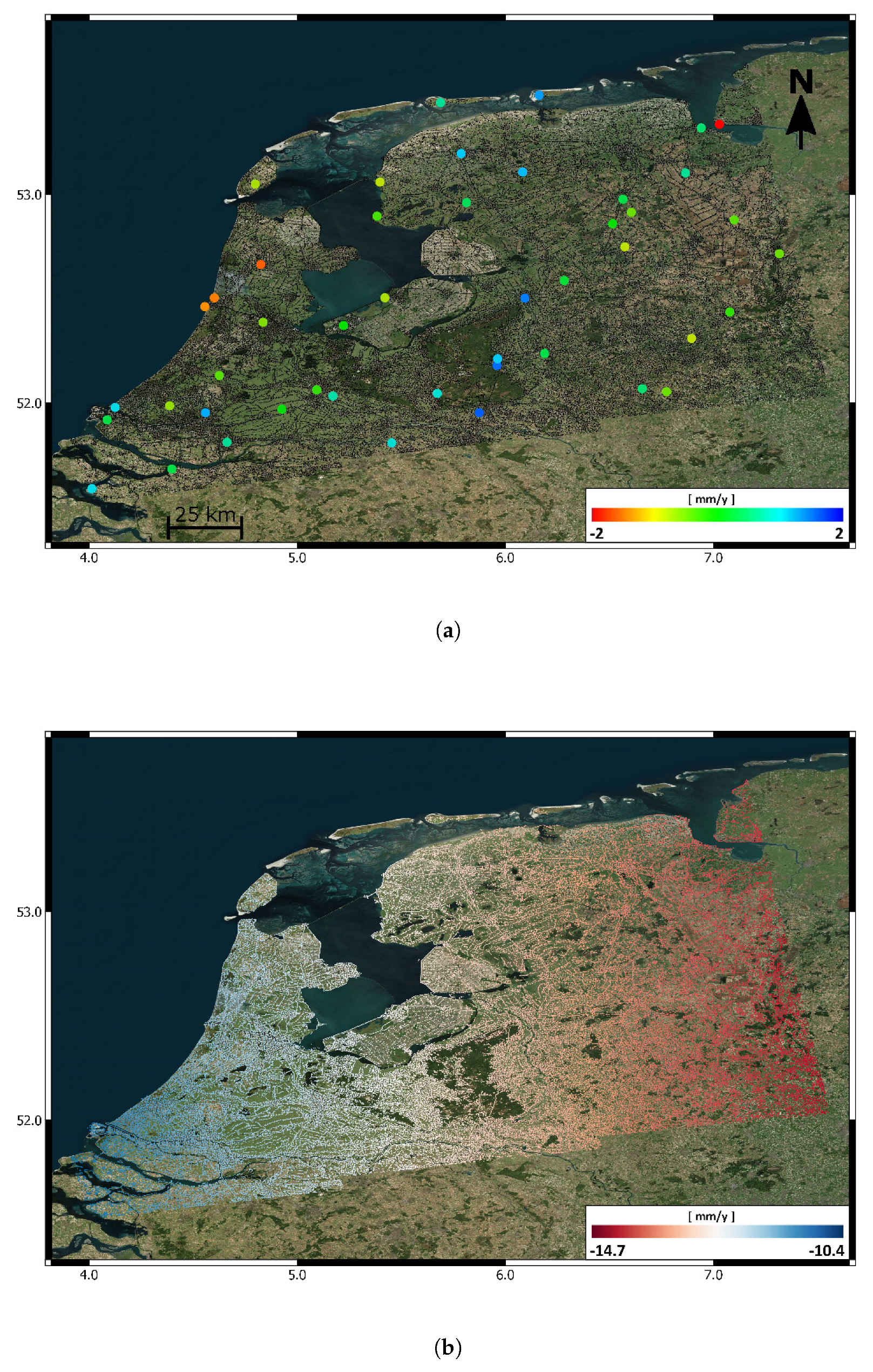
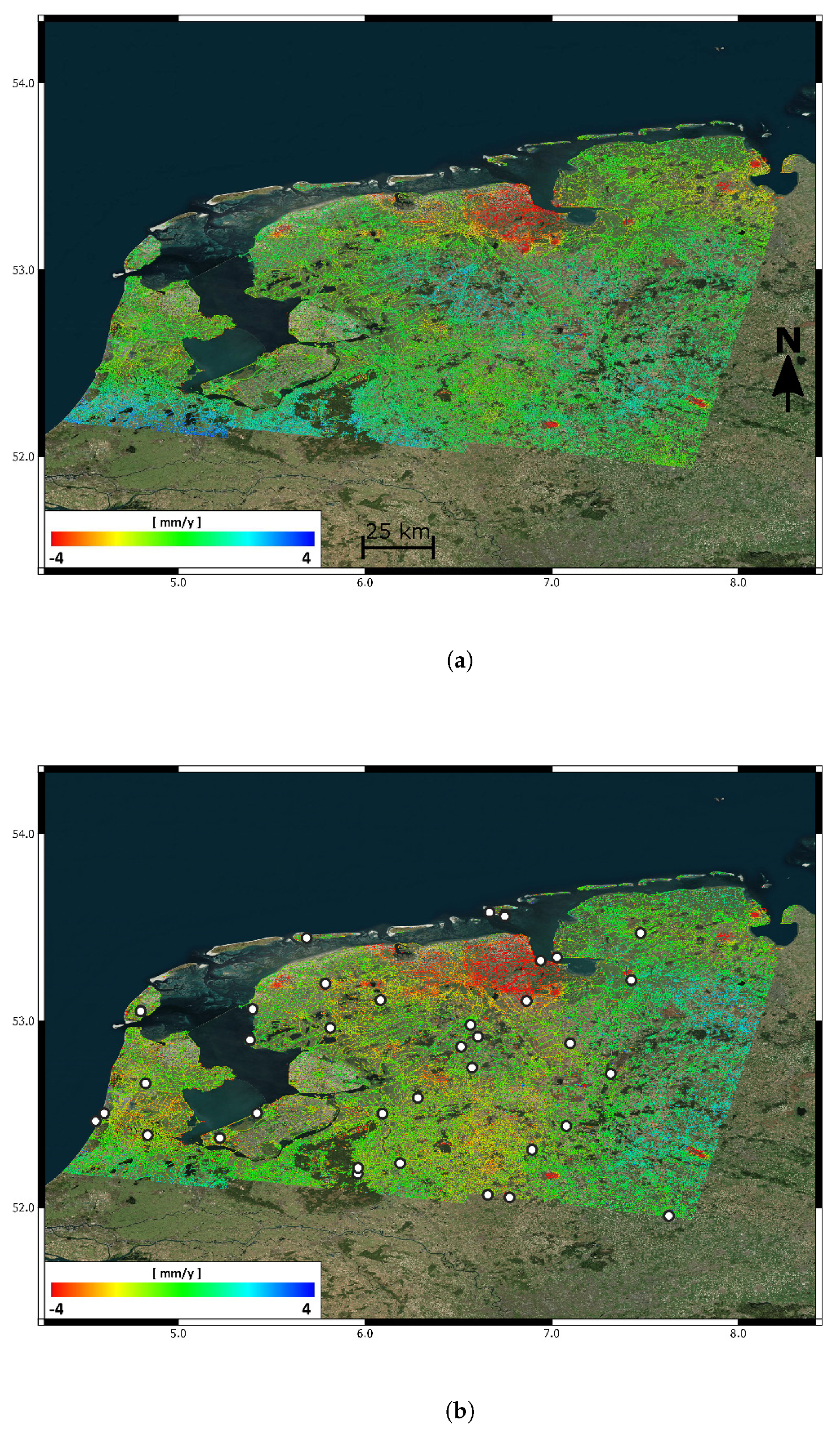
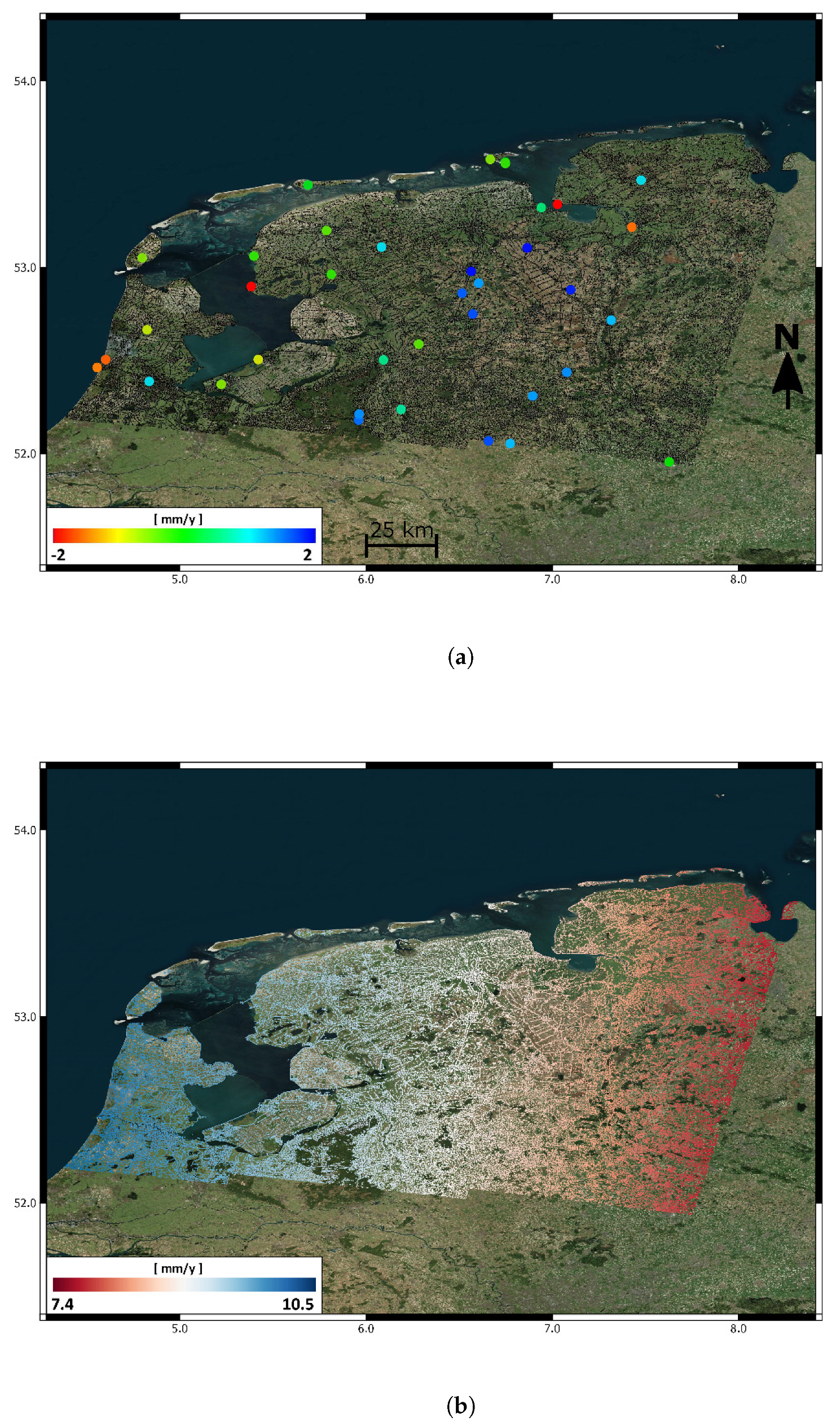
For the study, two Sentinel-1A/B datasets covering the northern part of the Netherlands (two stacks, ascending and descending) and the junction between the North Anatolian Fault and East Anatolian Fault (three stacks, descending) were used. The interferograms were computed, corrected for tropospheric delays using ECMWF ERA-5 (ECMWF Re-Analysis) data [8] and processed using the PSInSAR technique [26]. In order to preserve all wave-numbers of the deformation signal, no spatial high-pass filtering or polynomial detrending was performed on the final data. The technique described above was applied to the estimated deformation rates. As visible in Figure 6, Figure 7, Figure 8, Figure 9, Figure 10 and Figure 11, the method is able to retrieve the absolute motion while also mitigating the undesired residual atmospheric error, hence displaying all available spectral components in the deformation signal. Figure 7a, Figure 9a, and Figure 11a show that the residual zero-mean error is quite small, varying between mm/y. This can already be considered as a kind of validation of the InSAR data, whose accuracy is close to 1 mm/y.
For the reference measurements, the GNSS data processed by Nevada Geodetic Laboratories [27,28] were used. The correspondence GNSS/PSs for the calculation of vector was implemented by averaging all of the PS rates within a radius of 250 m from the GNSS station.
A further elucidation needs to be made. The reference system that describes SAR geometry (state vectors) does not account for continental drift making plate movement visible in the interferometric measurements, projected along the LoS. The GNSS data used for the calibration are also not continental drift compensated. Hence, the two data-sets can be considered “compatible”. After merging (also adding ), the data contains continental drift that could dominant the visualialization. Therefore, plate movement was compensated using the model in [29] to show movement relative to a specific plate (Eurasian). The removed motion is basically an overall offset of several mm/y, plus a light ramp due to the LoS projection of the horizontal motion. This is generally not necessary since it is only a representation issue, but it facilitates the interpretation of the results. For the sake of completeness, the removed model is also shown in Figure 7b, Figure 9b, and Figure 11b.
4.1. Netherlands Datasets
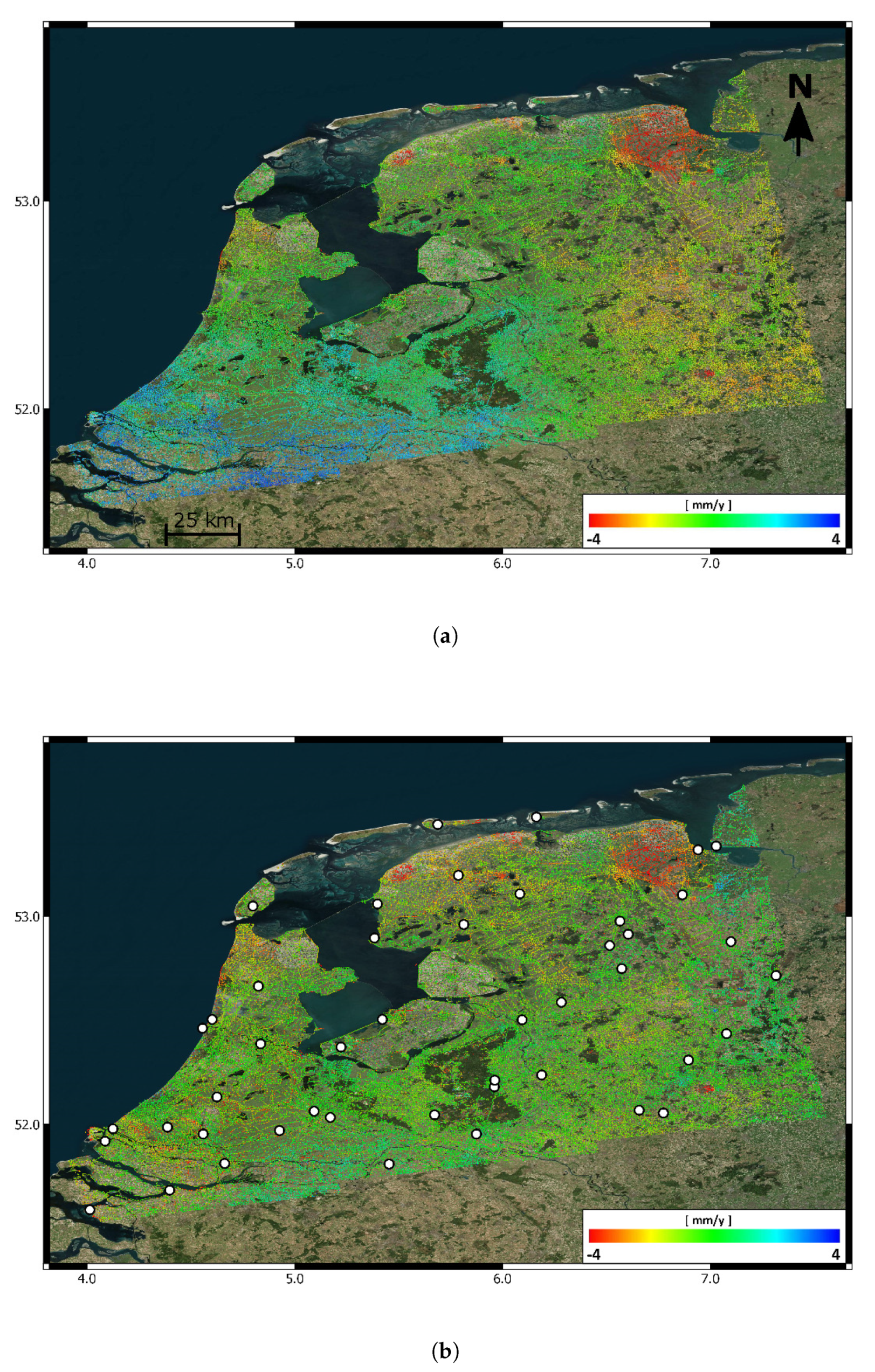
The systematic generation of deformation maps on a national scale using SAR interferometry has become more feasible, as missions like Sentinel-1 provide global coverage on a regular basis. Often, these kinds of services must be combined with existing geodetic measurements in order to make them integrated and comparable [21]. In this work, a typical example is provided where InSAR velocities covering a large area—acquired in descending and ascending passes—are combined with a consistent number of GNSS-derived velocities. The considered datasets are two Sentinel-1A/B stacks covering the northern part of the Netherlands. The area includes many examples of man-induced subsidences, such as in Groeningen [30]. The details of the dataset are described by Table 1. Observing the raw result of the PSI-processing, some spatially correlated deformation signals are visible when observing between mm/y. Since no large-scale deformation phenomena are expected in this area, such patterns must therefore be related to the residual atmospheric signal. In the area of interest, a considerably high number of GNSS data are available (see Table 1). The previously described methodology was applied to the data using the available GNSS measurements [27]. The results in Figure 6 and Figure 8 show how the technique permits the further reduction of the residual atmospheric error and the relation of every single PS measurement to the Eurasian plate only. Further information about the measured and the removed continental drift model is also available in Figure 7 and Figure 9. Since the ascending/descending data are now absolute, it would be possible to combine them directly using the error description provided in Equations (9)–(11).
4.2. North Anatolian Fault Dataset
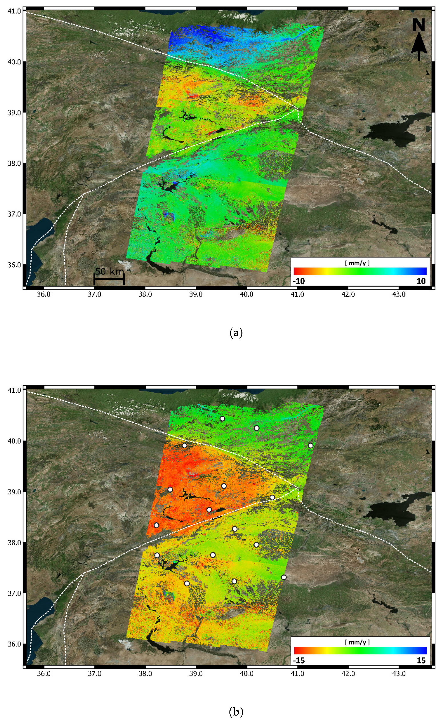
Applications related to the measurement of tectonic movements are the most challenging for InSAR. The requirement of an accuracy of 1 mm/y at more that 100 km (<10 nstrain) pushes the technique to its limits [5]. Notwithstanding, it has been demonstrated that, since actual SAR missions are characterized by very stable oscillators [31] and very good orbit knowledge [32,33], such numbers can be considered achievable. The major limitation is atmospheric effects. If the interferometric time series is not long enough, integration with other data would be necessary in order to fulfill the requirements at very large distances. Moreover, the possibility of referencing the measurements to standard reference systems (e.g., Eurasian Plate, etc.) would extend the usability of the final results.
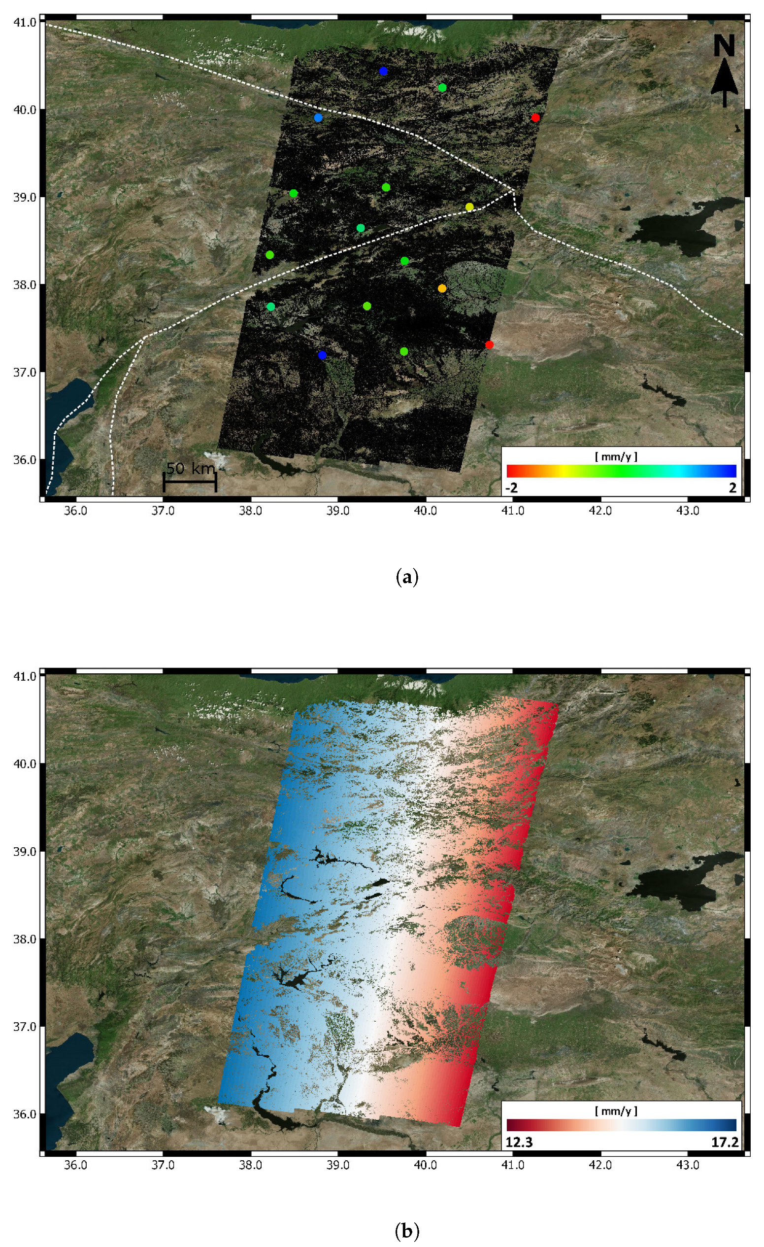
The technique must then also be demonstrated on an appropriate example for tectonics. The North Anatolian Fault was chosen, as it is a typical case study investigated by many geo-scientists using SAR interferometry [34,35]. The area of interest is covered by a Sentinel-1A/B stripe extending for more than 600 km in the along-track direction, see Table 2. In order to make the processing feasible, the stripe was divided into three frames. The three frames were processed independently using the PSInSAR technique. The area is very tectonically active and it is very important to preserve all scales of the measured deformation signal. Figure 10 displays the results together with a mapping of the main path of the North and East Anatolian Fault (dashed white line).
5. Conclusions
The results show how the technique is able to both remove dependence on the reference point and mitigate residual atmospheric errors present in the final InSAR results. The described methodology works under some straightforward assumptions on the input data that have to be considered:
- The GNSS/InSAR time series must overlapped in space and time,
- the 3D GNSS velocities and their variances are known, and
- the motion of the GNSS station should be representative of the motion of the area.
The method was studied on both simulated and real data. Simulations show that even with a reduced set of GNSS stations it is possible to retrieve the absolute motion with good accuracy. On the other hand, the capability of the approach to mitigate residual atmospheric errors depends both on the GNSS station density and the spatial correlation of the errors. In order to provide some numbers, the error was modeled as an process with a correlation length of 60 km and variable overall variance. Such numbers were used because they match with the experiments. Two real test cases were then processed to demonstrate the approach by trying to address applications that should benefit from the technique. The results are promising and open the door to an accurate cross-validation between GNSS/InSAR. The extension of the approach to time series would also be interesting, merging InSAR phases with continuous GNSS measurements. The approach could be conceptually equivalent, since the deformation rates are just a scaling of the single-phase measurements, but the spatial covariance of each interferogram would be needed.
For the sake of precision, it is noted that estimation of is also generally possible using only InSAR data. The key parameter to be considered here is indeed the length of the time series . Theoretically speaking, with a long time series, it is possible to robustly estimate the motion of the reference point by comparing the interferometric deformation rates with the rates estimated from group delays, using co-registration shifts or the PS positions [36,37]. Moreover, if is large enough, the residual atmospheric effects are also sufficiently small to fulfill even the strict requirements [8] set by applications aimed at measuring tectonic movements [5]. Notwithstanding, if is not large enough to fulfill the accuracy requirements at large distances, then merging with GNSS is necessary.
In general, it is possible to conclude that the developed method helps to increase, when necessary, the accuracy of InSAR over large distances [8]. The final product has the spatial coverage of InSAR, and is an optimal combination of InSAR and GNSS information based on the knowledge of the error statistics. This preserves all scales of the deformation signal and also allows characterization of the final product error.
Author Contributions
Conceptualization, A.P., F.R.G. and R.B.; Methodology, A.P.; Software, A.P. and F.R.G.; Investigation, A.P.; Writing—Original Draft Preparation, A.P.; Writing—Review and Editing, A.P. and R.B. All authors have read and agreed to the published version of the manuscript.
Funding
This research received no external funding.
Acknowledgments
The authors would like to thank Ekaterina Tymofyeyeva for the suggestions that helped improving the manuscript.
Conflicts of Interest
The authors declare no conflict of interest.
Abbreviations
The following abbreviations are used in this manuscript:
| SAR | Synthetic Aperture Radar |
| InSAR | Synthetic Aperture Radar Interferometry |
| PS | Persistent Scatterer |
| PSI | Persistent Scatterers Interferometry |
| LoS | Line of Sight |
| GNSS | Global Navigation Satellite System |
| ECMWF | European Centre for Medium-Range Weather Forecasts |
| ERA | ECMWF Re-Analysis |
References
- Rosen, P.; Hensley, S.; Joughin, I.; K.Li, F.; Madsen, S.; Rodriguez, E.; Goldstein, R.M. Synthetic aperture radar interferometry. Proc. IEEE 2000, 88, 333–382. [Google Scholar] [CrossRef]
- Rosen, P.A.; Hensley, S.; Zebker, H.A.; Webb, F.H.; Fielding, E.J. Surface deformation and coherence measurements of Kilauea Volcano, Hawaii, from SIR-C radar interferometry. J. Geophys. Res. Planets 1996, 101, 23109–23125. [Google Scholar] [CrossRef]
- Gray, A.L.; Mattar, K.E.; Sofko, G. Influence of ionospheric electron density fluctuations on satellite radar interferometry. Geophys. Res. Lett. 2000, 27, 1451–1454. [Google Scholar] [CrossRef]
- Hanssen, R. Radar Interferometry: Data Interpretation and Error Analysis; Springer: Dordrecht, The Netherlands, 2001. [Google Scholar]
- Wright, T.J. The earthquake deformation cycle. Astron. Geophys. 2016, 57, 4.20–4.26. [Google Scholar] [CrossRef]
- Torres, R.; Snoeij, P.; Geudtner, D.; Bibby, D.; Davidson, M.; Attema, E.; Potin, P.; Rommen, B.; Floury, N.; Brown, M.; et al. GMES Sentinel-1 mission. Remote Sens. Environ. 2012, 120, 9–24. [Google Scholar] [CrossRef]
- Moreira, A.; Krieger, G.; Hajnsek, I.; Papathanassiou, K.; Younis, M.; Lopez-Dekker, P.; Huber, S.; Villano, M.; Pardini, M.; Eineder, M.; et al. Tandem-L: A Highly Innovative Bistatic SAR Mission for Global Observation of Dynamic Processes on the Earth’s Surface. IEEE Geosci. Remote Sens. Mag. 2015, 3, 8–23. [Google Scholar] [CrossRef]
- Gonzalez, F.R.; Parizzi, A.; Brcic, R. Evaluating the impact of geodetic corrections on interferometric deformation measurements. In Proceedings of the EUSAR 2018: 12th European Conference on Synthetic Aperture Radar, Aachen, Germany, 4–7 June 2018; pp. 1–5. [Google Scholar]
- Gudmundsson, S.; Carstensen, J.M.; Sigmundsson, F. Unwrapping ground displacement signals in satellite radar interferograms with aid of GPS data and MRF regularization. IEEE Trans. Geosci. Remote Sens. 2002, 40, 1743–1754. [Google Scholar] [CrossRef]
- Shanker, A.P.; Zebker, H. Edgelist phase unwrapping algorithm for time series InSAR analysis. JOSA A 2010, 27, 605–612. [Google Scholar] [CrossRef]
- Wei, M.; Sandwell, D.; Smith-Konter, B. Optimal combination of InSAR and GPS for measuring interseismic crustal deformation. Adv. Space Res. 2010, 46, 236–249. [Google Scholar] [CrossRef]
- Tong, X.; Sandwell, D.; Smith-Konter, B. High-resolution interseismic velocity data along the San Andreas fault from GPS and InSAR. J. Geophys. Res. Solid Earth 2013, 118, 369–389. [Google Scholar] [CrossRef] [Green Version]
- Farolfi, G.; Bianchini, S.; Casagli, N. Integration of GNSS and Satellite InSAR Data: Derivation of Fine-Scale Vertical Surface Motion Maps of Po Plain, Northern Apennines, and Southern Alps, Italy. IEEE Trans. Geosci. Remote Sens. 2019, 57, 319–328. [Google Scholar] [CrossRef]
- Wang, H.; Wright, T. Satellite geodetic imaging reveals internal deformation of western Tibet. Geophys. Res. Lett. 2012, 39. [Google Scholar] [CrossRef] [Green Version]
- Catalão, J.; Nico, G.; Hanssen, R.; Catita, C. Merging GPS and atmospherically corrected InSAR data to map 3-D terrain displacement velocity. IEEE Trans. Geosci. Remote Sens. 2011, 49, 2354–2360. [Google Scholar] [CrossRef] [Green Version]
- Bekaert, D.; Segall, P.; Wright, T.; Hooper, A. A network inversion filter combining GNSS and InSAR for tectonic slip modeling. J. Geophys. Res. Solid Earth 2016, 121, 2069–2086. [Google Scholar] [CrossRef] [Green Version]
- Mahapatra, P.S.; Samiei-Esfahany, S.; Van der Marel, H.; Hanssen, R.F. On the use of transponders as coherent radar targets for SAR interferometry. IEEE Trans. Geosci. Remote Sens. 2014, 52, 1869–1878. [Google Scholar] [CrossRef]
- Mahapatra, P.; Van der Marel, H.; Van Leijen, F.; Samiei-Esfahany, S.; Klees, R.; Hanssen, R. InSAR datum connection using GNSS-augmented radar transponders. J. Geod. 2018, 92, 21–32. [Google Scholar] [CrossRef] [Green Version]
- Mahapatra, P.S.; Samiei-Esfahany, S.; Hanssen, R.F. Geodetic Network Design for InSAR. IEEE Trans. Geosci. Remote Sens. 2015, 53, 3669–3680. [Google Scholar] [CrossRef]
- Jonsson, S.; Zebker, H.; Segall, P.; Amelung, F. Fault Slip Distribution of the 1999 Mw 7.1 Hector Mine, California, Earthquake, Estimated from Satellite Radar and GPS Measurements. Bull. Seismol. Soc. Am. 2002, 92, 1377–1389. [Google Scholar] [CrossRef]
- Kalia, A.; Frei, M.; Lege, T. A Copernicus downstream-service for the nationwide monitoring of surface displacements in Germany. Remote Sens. Environ. 2017, 202, 234–249. [Google Scholar] [CrossRef]
- Fattahi, H.; Amelung, F. InSAR bias and uncertainty due to the systematic and stochastic tropospheric delay. J. Geophys. Res. Solid Earth 2015, 120, 8758–8773. [Google Scholar] [CrossRef] [Green Version]
- Cong, X.; Balss, U.; Eineder, M.; Fritz, T. Imaging geodesy—Centimeter-level ranging accuracy with TerraSAR-X: An update. IEEE Geosci. Remote Sens. Lett. 2012, 9, 948–952. [Google Scholar] [CrossRef] [Green Version]
- Cong, X. SAR Interferometry for Volcano Monitoring: 3D-PSI Analysis and Mitigation of Atmospheric Refractivity. Ph.D. Thesis, Technische Universität München, München, Germany, 2014. [Google Scholar]
- Proakis, J.; Manolakis, D. Digital Signal Processing; Prentice Hall: Upper Saddle River, NJ, USA, 2006. [Google Scholar]
- Ferretti, A.; Prati, C.; Rocca, F. Permanent scatterers in SAR interferometry. IEEE Trans. Geosci. Remote Sens. 2001, 39, 8–20. [Google Scholar] [CrossRef]
- MIDAS Velocity Fields. Available online: http://geodesy.unr.edu/ (accessed on 1 October 2018).
- Blewitt, G.; Kreemer, C.; Hammond, W.C.; Gazeaux, J. MIDAS robust trend estimator for accurate GPS station velocities without step detection. J. Geophys. Res. Solid Earth 2016, 121, 2054–2068. [Google Scholar] [CrossRef]
- Rouby, H.; Métivier, L.; Rebischung, P.; Altamimi, Z.; Collilieux, X. ITRF2014 plate motion model. Geophys. J. Int. 2017, 209, 1906–1912. [Google Scholar] [CrossRef]
- Ketelaar, V.G. Satellite Radar Interferometry: Subsidence Monitoring Techniques; Springer Science & Business Media: Berlin/Heidelberg, Germany, 2009; Volume 14. [Google Scholar]
- Larsen, Y.; Marinkovic, P.; Dehls, J.F.; Perski, Z.; Hooper, A.J.; Wright, T.J. The Sentinel-1 constellation for InSAR applications: Experiences from the InSARAP project. In Proceedings of the 2017 IEEE International Geoscience and Remote Sensing Symposium (IGARSS), Fort Worth, TX, USA, 23–28 July 2017; pp. 5545–5548. [Google Scholar]
- Yoon, Y.T.; Eineder, M.; Yague-Martinez, N.; Montenbruck, O. TerraSAR-X Precise Trajectory Estimation and Quality Assessment. IEEE Trans. Geosci. Remote Sens. 2009, 47, 1859–1868. [Google Scholar] [CrossRef]
- Peter, H.; Jäggi, A.; Fernández, J.; Escobar, D.; Ayuga, F.; Arnold, D.; Wermuth, M.; Hackel, S.; Otten, M.; Simons, W.; et al. Sentinel-1A–First precise orbit determination results. Adv. Space Res. 2017, 60, 879–892. [Google Scholar] [CrossRef]
- Cakir, Z.; Ergintav, S.; Akoğlu, A.M.; Çakmak, R.; Tatar, O.; Meghraoui, M. InSAR velocity field across the North Anatolian Fault (eastern Turkey): Implications for the loading and release of interseismic strain accumulation. J. Geophys. Res. Solid Earth 2014, 119, 7934–7943. [Google Scholar] [CrossRef] [Green Version]
- Hussain, E.; Wright, T.J.; Walters, R.J.; Bekaert, D.P.; Lloyd, R.; Hooper, A. Constant strain accumulation rate between major earthquakes on the North Anatolian Fault. Nat. Commun. 2018, 9, 1392. [Google Scholar] [CrossRef]
- Madsen, S.N.; Zebker, H.A.; Martin, J. Topographic mapping using radar interferometry: Processing techniques. IEEE Trans. Geosci. Remote Sens. 1993, 31, 246–256. [Google Scholar] [CrossRef]
- Eineder, M.; Minet, C.; Steigenberger, P.; Cong, X.; Fritz, T. Imaging Geodesy—Toward Centimeter-Level Ranging Accuracy With TerraSAR-X. IEEE Trans. Geosci. Remote Sens. 2011, 49, 661–671. [Google Scholar] [CrossRef]
Figure 1.
Flow chart of the proposed method.

Figure 2.
Examples of an exponential fitting of the deformation rate variograms. The black dots represent the estimated variogram and the bold red line represents the estimated model. The variograms in (a) and (b) refer to the stacks 123/2 and 123/3 of the North Anatolian Fault data set respectively, see Section 4.2.

Figure 3.
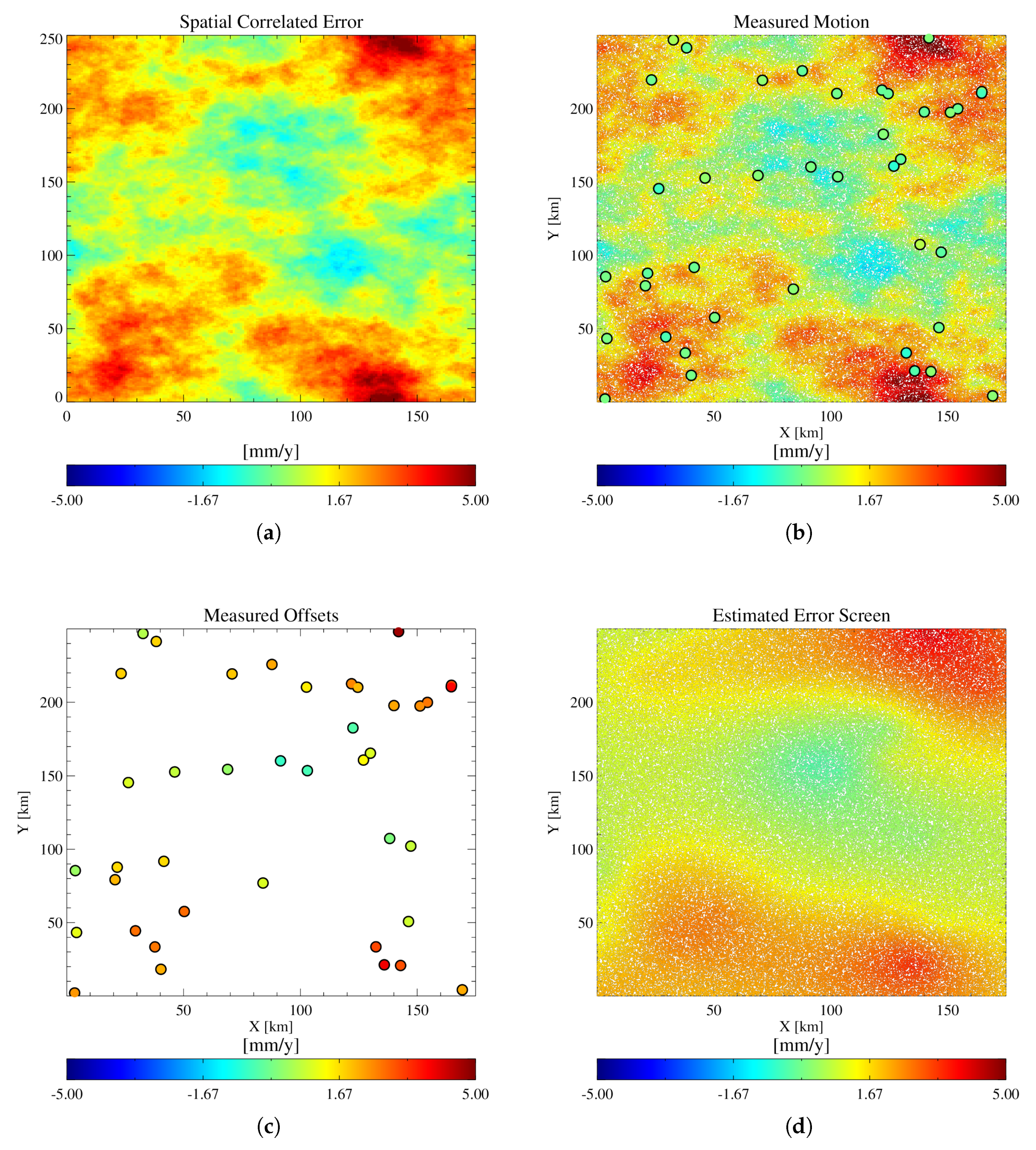
The Figure shows an example of the framework used for the simulations. The simulated motion is 0 over the entire scene. In (a), the simulated spatially correlated noise is depicted. In (b), the dense Synthetic Aperture Radar Interferometry (InSAR) measurements and the coarse Global Navigation Satellite System (GNSS; large dots, atmosphere-free) are depicted. In (c), the measured offsets InSAR/GNSS () are depicted. In (d), the estimated error screen to be removed from (b) is depicted. In (e), the final results obtained by calibrating (b) with (d) are depicted. In (f), the estimated error for the merged product is depicted.
Figure 3.
The Figure shows an example of the framework used for the simulations. The simulated motion is 0 over the entire scene. In (a), the simulated spatially correlated noise is depicted. In (b), the dense Synthetic Aperture Radar Interferometry (InSAR) measurements and the coarse Global Navigation Satellite System (GNSS; large dots, atmosphere-free) are depicted. In (c), the measured offsets InSAR/GNSS () are depicted. In (d), the estimated error screen to be removed from (b) is depicted. In (e), the final results obtained by calibrating (b) with (d) are depicted. In (f), the estimated error for the merged product is depicted.


Figure 4.
Performance simulations in retrieving carried out with different atmospheric noise sills: (a) 2 mm/y and (b) 9 mm/y.
Figure 4.
Performance simulations in retrieving carried out with different atmospheric noise sills: (a) 2 mm/y and (b) 9 mm/y.

Figure 5.
Performance simulations in retrieving carried out with different atmospheric noise sills: (a) 2 mm/y and (b) 9 mm/y.
Figure 5.
Performance simulations in retrieving carried out with different atmospheric noise sills: (a) 2 mm/y and (b) 9 mm/y.

Figure 6.
Results for the ascending Holland stack (a) before and (b) after performing merging with GNSS data. In (b), the GNSS stations used are displayed with black–white circles.
Figure 6.
Results for the ascending Holland stack (a) before and (b) after performing merging with GNSS data. In (b), the GNSS stations used are displayed with black–white circles.

Figure 7.
Results for the ascending Holland stack, showing the measured and color-coded in (a) and the removed continental drift screen in (b).
Figure 7.
Results for the ascending Holland stack, showing the measured and color-coded in (a) and the removed continental drift screen in (b).

Figure 8.
Results for the descending Holland stack, showing (a) before and (b) after performing merging with GNSS data. In (b), the GNSS stations used are displayed with black–white circles.
Figure 8.
Results for the descending Holland stack, showing (a) before and (b) after performing merging with GNSS data. In (b), the GNSS stations used are displayed with black–white circles.

Figure 9.
Results for the descending Holland stack, showing (a) the measured and color-coded and (b) the removed continental drift screen.
Figure 9.
Results for the descending Holland stack, showing (a) the measured and color-coded and (b) the removed continental drift screen.

Figure 10.
Results for the North Anatolian Fault (a) before and (b) after performing merging with GNSS data. In (b), the GNSS stations used are displayed with black–white circles and the fault lines are displayed using a white dashed line.
Figure 10.
Results for the North Anatolian Fault (a) before and (b) after performing merging with GNSS data. In (b), the GNSS stations used are displayed with black–white circles and the fault lines are displayed using a white dashed line.

Figure 11.
Results for the North Anatolian Fault, showing (a) the measured and color-coded and (b) the removed continental drift screen.
Figure 11.
Results for the North Anatolian Fault, showing (a) the measured and color-coded and (b) the removed continental drift screen.


Table 1.
Netherlands Dataset.
| Track | Orbit | Acquisitions | Time [years] | GNSS Stations |
|---|---|---|---|---|
| 088 | ASCE | 140 | 3.4 | 47 |
| 037 | DESCE | 122 | 3.0 | 37 |
Table 2.
North Anatolian Fault Dataset.
| Track | Orbit | Acquisitions | Time [years] | GNSS Stations |
|---|---|---|---|---|
| DESCE | 134 | 3.3 | 5 | |
| DESCE | 134 | 3.3 | 9 | |
| DESCE | 134 | 3.3 | 4 |
© 2020 by the authors. Licensee MDPI, Basel, Switzerland. This article is an open access article distributed under the terms and conditions of the Creative Commons Attribution (CC BY) license (http://creativecommons.org/licenses/by/4.0/).
Share and Cite
MDPI and ACS Style
Parizzi, A.; Rodriguez Gonzalez, F.; Brcic, R. A Covariance-Based Approach to Merging InSAR and GNSS Displacement Rate Measurements. Remote Sens. 2020, 12, 300. https://0-doi-org.brum.beds.ac.uk/10.3390/rs12020300
AMA Style
Parizzi A, Rodriguez Gonzalez F, Brcic R. A Covariance-Based Approach to Merging InSAR and GNSS Displacement Rate Measurements. Remote Sensing. 2020; 12(2):300. https://0-doi-org.brum.beds.ac.uk/10.3390/rs12020300
Chicago/Turabian StyleParizzi, Alessandro, Fernando Rodriguez Gonzalez, and Ramon Brcic. 2020. "A Covariance-Based Approach to Merging InSAR and GNSS Displacement Rate Measurements" Remote Sensing 12, no. 2: 300. https://0-doi-org.brum.beds.ac.uk/10.3390/rs12020300
Note that from the first issue of 2016, this journal uses article numbers instead of page numbers. See further details here.