An Adaptive Hierarchical Detection Method for Ship Targets in High-Resolution SAR Images


National Lab of Radar Signal Processing, Xidian University, Xi’an 710071, China
*
Author to whom correspondence should be addressed.
Remote Sens. 2020, 12(2), 303; https://0-doi-org.brum.beds.ac.uk/10.3390/rs12020303
Submission received: 4 December 2019
/
Revised: 10 January 2020
/
Accepted: 15 January 2020
/
Published: 17 January 2020
(This article belongs to the Section Remote Sensing Image Processing)
Abstract
:With the improvement of image resolution in synthetic aperture radars (SARs), sea clutter characteristics become more complex, which poses new challenges to traditional ship target detection missions. In this paper, to detect ship targets quickly and efficiently in a complex background, we propose an adaptive hierarchical detection method based on a coarse-to-fine mechanism. This method constructs a new visual attention mechanism to strengthen ship targets and obtain the candidate targets adaptively by the means dichotomy method. On this basis, the precise detection results of the targets are obtained using the speed block kernel density estimation method, which maintains constant false alarm characteristics. Compared with existing methods, the adaptive hierarchical detection method has simple, fast, and accurate characteristics. Experiments based on GF-III satellite and airborne SAR datasets are presented to demonstrate the effectiveness of the proposed method.
1. Introduction
Ocean monitoring that uses earth observation data includes many activities and applications that support different needs: sustainable fishing, marine ecosystem protection, natural resource extraction, commerce, trade, etc. Regarding maritime traffic, the world fleet of cargo carrying vessels has increased from 77,500 vessels in 2008 to some 100,000 vessels in 2018, comprising a total capacity of more than 2100 million deadweight tonnage [1]. Consequently, as an important maritime application, ship detection plays an increasingly essential role in marine monitoring and maritime traffic supervision.
Synthetic aperture radars (SARs) have the unique capability of earth observation in all-weather conditions, regardless whether it is day or night. Due to the variation of backscatter properties of different objects, SAR images can provide discriminative features for reliable scene understanding and interpretation, which is the basic principle of SAR image ship detection [2]. With the rapid development of SAR technology, such as TerraSAR-X, RADARSAT–2, and GF-III, it is no longer difficult to acquire high-resolution SAR images, which has promoted the application of SAR images in the field of ship target detection [3].
Generally, the ship detection methods for SAR images focus on a constant false alarm rate (CFAR) detector. The performance of CFAR detectors depends on the design of the sliding window structure, the statistical modeling of clutter distribution, and the estimation of model parameters [2]. Over the years, a great number of window structures have been designed under the CFAR framework to deal with speckle noise and complex scenes, such as the famous two-parameter CFAR [4], ordered-statistic [5], cell-averaging [6], etc. Due to the constraint of the low-resolution SAR images in the early stage, most of the early ship detection methods focus on point targets. Moreover, sea clutter characteristics can be assumed to have a simple Gauss distribution. As the resolution increases, the structure becomes more obvious with targets occupying more pixels, and the characteristics of sea clutter also become more complex, which induces severe challenges for traditional detection methods.
Confronted with the new characteristics of high-resolution SAR images, the conventional detectors suffer from severe performance deterioration in the multitarget situation or nonhomogeneous backgrounds. To ameliorate the performance of detection, lots of literature has brought forward improved methods. Some research has focused on the design of the detection mechanism, which is a significant factor and affects detection performance. Leng et al. [7] proposed a detection window design method, which can adjust the window size according to radar parameters. Ao et al. proposed a multiscale CFAR detection method [8], which is used in coastal areas. However, because of its large-scale detector, it may provide too many candidate targets in a complex environment, which generates more false alarms. Yu et al. [9] used a structural-information-based superpixel method to detect ship targets, which showed good performance. However, the selection mechanism of the clutter superpixel block is not stable and its sliding window detection scheme causes large computational burdens. Tao et al. [10] made an improvement to the superpixel by adopting weighted information entropy to extract candidate superpixel blocks and using their neighborhood superpixels for parameter estimation, which reduced the amount of calculation. However, the Gauss distribution clutter model chosen in this method suffers from serious mismatch risk.
In addition to the design of the detection mechanism, another important factor affecting detection performance is the construction of the sea clutter model. Researchers have explored many clutter distribution models based on experience or central limit theorem, such as generalized k distribution [11], Weibull distribution [12], generalized Gamma distribution () [13], etc. These models have good fitting effects under specific sea conditions. However, with the increasing complexity of the models, the parameter estimation becomes a challenge and even constrains practical application of CFAR technology [2]. Moreover, various sea conditions and different radar system parameters influence the clutter distribution. Therefore, there is a high risk of mismatch if we simply choose a specific clutter model to characterize the clutter distribution, which is inaccurate and affects the detection result.
To avoid the error caused by model mismatch, some researchers have explored detection methods based on spatial correlation and structural characteristics. Wang et al. [2] proposed a method that combined attention selection mechanism, which adopts the random forest method based on image blocks with contour information. However, the segmentation size of image blocks cannot be adaptively selected, so it is difficult to obtain candidate targets steadily at different resolutions. Salembier et al. [1] proposed a ship detection method for SAR images based on Maxtree representation and graph signal processing, in which radiometric as well as geometric attributes are evaluated and associated with the Maxtree nodes. Moreover, with the wide application of deep learning in the field of computer vision, researchers propose a variety of SAR ship detection methods based on deep learning. To further improve the detection performance, Lin et al. [14] proposed a new network architecture by using the squeeze and excitation mechanism. Jiao et al. [3] proposed a densely connected multiscale neural network based on a faster RCNN framework to realize multiscale SAR ship detection. Deep learning methods have achieved good results in the detection of nearshore ship targets, which is a promising direction. However, in the present experiment, we noticed that it needs a mass of manually preprocessed data to train a robust detection model. When the detection scene changes, how to guarantee the detection performance still need to be further studied.
In sum, this paper aims to improve the ship detection performance and solve the problems in the present methods that can be summarized as follows: (a) the fixed detection window methods are difficult to extract the target completely in the multi-size detection condition; (b) the conventional pixel-by-pixel detection methods are too heavy and time-consuming to be applied in large scenes; (c) there is a risk of mismatch in clutter models under complex sea conditions; (d) the detection methods based on deep learning cannot guarantee the performance when the detection scene changes or targets are vague. In order to solve previous problems and improve the detection quality, an adaptive hierarchical detection method is proposed in this paper. First, an improved visual attention mechanism combining the image domain with the frequency domain is presented, which can effectively suppress the residual coastal area after land–sea segmentation and highlight the ship target at the same time. Then, the mean dichotomy method is introduced to adaptively obtain the candidate target regions, which replaces the hard threshold design of artificial participation in traditional methods. Finally, to eliminate the mismatch risk of the clutter distribution model under complex sea conditions, a nonparametric block kernel density estimation (BKDE) method is adopted. Moreover, to modify the shortcomings of the kernel density estimation (KDE), the frequency domain acceleration method is studied.
The paper is organized as follows. The traditional detection method is analyzed in Section 2. Section 3 presents a detailed description of the adaptive hierarchical detection method. Then, the comparative experimental results with real SAR images are provided and analyzed in Section 4. Finally, the conclusion of the paper is summarized in Section 5.
2. The Analyses of the Traditional Method
The common situation in the maritime target detection is the vast sea area and the small number of ships, so the most significant issue is to select the region of interest (ROI) and extract the target in the broad field quickly. Confronted with this situation, the sliding window detection methods represented by the traditional two-parameter CFAR detector [4] have the following shortcomings. First, the size of the detected ship is requisite to determine the size of the protection window, which applies to a certain class of targets in locally uniform clutter conditions [15]. Yet when ship targets with heterogeneous sizes appear in SAR images, the single-size window has the risk that target pixels leak to the background window affecting the detection threshold. It will increase the possibility of losing target pixels and the detected targets may have holes and fractures [10,16]. Besides, ship targets often occupy a small part of pixels in the image, but the sliding window technique traverses each pixel in the image, which undoubtedly causes excessive redundancy calculation. Furthermore, Gaussian distribution is commonly used as the sea clutter model in traditional methods, which has a high mismatch risk in high-resolution images.
One valid way to solve these problems is to introduce the coarse-to-fine detection mechanism. In this mechanism, a fast but coarse detector is utilized to select the candidate targets, then a more accurate detector is adopted to complete the precise detection of candidate targets. In this way, it can effectively solve the contradiction between efficiency and accuracy, as well as avoid the risk of target fracture brought about by the fixed window method in multi-size cases. It should be noted that the coarse-to-fine detection mechanism is used in the detection stage, which does not contain the discrimination operator.
This idea of coarse-to-fine has been adopted by processes explained in the literature [2]. The model in this paper is carried out by establishing the random forest model of scarcity measurement and using the segmentation priority provided by graph cutting. Based on the random forest map of SAR image, the accurate detection results of ship targets are obtained by the active contour method. Potentialities of the recent Global Navigation Satellite System-Reflectometry (GNSS-R) technology in the detection of ship targets over the sea in near real-time are explored by Simone et al. [17]. The method consists of four steps: preprocessing, pre-screening, selection, and geolocation. Experiment on actual UK TechDemoSat–1 data verifies the effectiveness. This method still requires traversing the entire data in the pre-screening step. Other studies [18] describe a software platform dedicated to sea surveillance, capable of detecting and identifying illegal maritime traffic. This platform results from the cascade pipeline of several image processing algorithms that input radar or optical imagery captured by satellite-borne sensors and try to identify vessel targets in the scene and provide quantitative descriptors about their shape and motion. Ship detection in this method uses a fixed shape detection window, which has the risk that target pixels leak to the background window affecting the detection threshold.
Another effective coarse-to-fine detection method is to use the superpixel segmentation method to get the clustering regions of targets and then carry out accurate detection results on this basis. Yu et al. [9] proposed a target detection method based on the superpixel segmentation technology, which uses structure information to choose the clutter superpixels and adopts a sliding window scheme. A modified approach presented by leng et al. [10] employs weighted information entropy and kernel density estimation to extract candidate superpixel blocks, then uses neighborhood superpixel blocks to estimate the sea clutter model parameters, which improves the detection performance effectively.
At present, by introducing the deep learning, lots of improved ship detection methods are proposed by researchers. These detection methods based on deep learning can be divided into two directions. One is the one stage detection method represented by the Yolo series [19,20,21]. These methods use the convolutional neural network to extract the feature map of the detection area and then directly return the target position and category through the feature map. The other is the two-stage methods represented by RCNN series [22,23,24], which uses convolution neural networks to get the feature map, then uses a region proposal network (RPN) to get ROI areas. Finally, a network is designed to judge the ROI areas to get the precise results. The essence of these deep-learning-based methods is also a kind of detection mechanism of coarse-to-fine.
Although the coarse-to-fine ship target detection method achieves better detection results than the conventional method, there are still some problems that need to be solved. First, the target detection methods based on the visual attention mechanism face the contradiction between the effect of the saliency map and the computational load. Second, the detection methods based on the saliency map loses the criterion of the constant false alarm and most of the methods use the artificial threshold, which is difficult to deal with the change of the detection scene. Third, the calculation of the superpixel segmentation methods are heavy and the simulation results indicate that the segmentation grid almost consists of the initial grid. Hence, it is worthy of studying a simpler and less computational burden method. Fourth, although using the neighborhood pixels of candidate regions can avoid the model error caused by uniform parameter estimation in large scenes, the model mismatch is still unavoidable because of the use of a specific model.
To solve the above problems, this paper makes efforts in the following aspects: (a) a more lightweight visual attention mechanism; (b) an adaptive threshold selection method; (c) the design of the detection window that can adapt to multi-scale situation; (d) a nonparametric clutter modeling method; (e) an acceleration method of the nonparametric model. The detailed description of the method is given below.
3. Adaptive Hierarchical Ship Target Detection
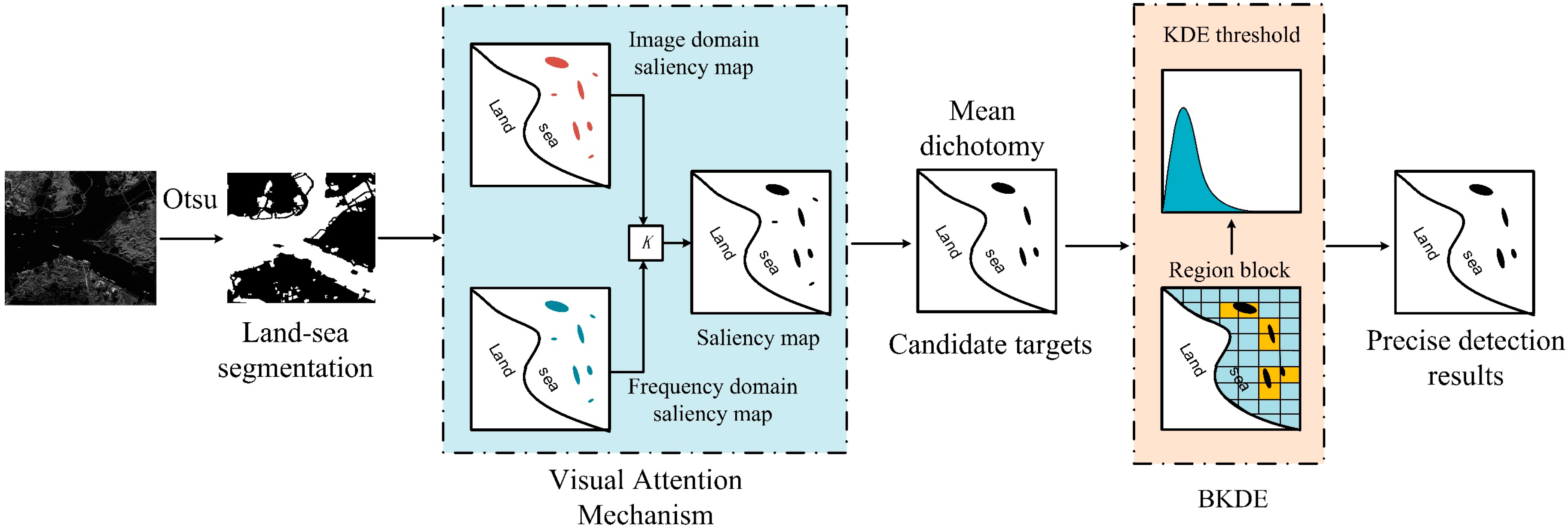
The basic process of ship target detection includes three parts: land–sea segmentation, ship detection, and discrimination [25,26]. This paper mainly focuses on the ship detection step. Considering the integrity of the proposed method, this section includes the content of land segmentation but only gives a brief introduction. The adaptive hierarchical ship target detection method adopts the idea of coarse-to-fine detection. First, the sea surface region is obtained by the land–sea segmentation technique. Then, the saliency map is generated by the block-based speed saliency detection method, which combines the image domain with the frequency domain. On this basis, the target candidate regions are extracted by the mean dichotomy method. Finally, to obtain the refined detection results of the ship targets, the block kernel density estimation method is utilized. The specific operations are as follows.
3.1. Land–Sea Segmentation Pretreatment
Since a large number of false alarms are often generated in the land area during the detection process, and the handling of these false alarms greatly increases the burden on the system, land–sea segmentation is an essential pretreatment.
The purpose of the land–sea segmentation is to eliminate the influence of land, island, and other areas on detection. Common land–sea segmentation methods include the methods based on Geographic Information System (GIS) [10], snake model [26], maximum class variance method (Otsu) [27], etc. GIS can provide the geographic information of observation areas, but the orbit parameters of SAR sensors are not always accurately known and there may be errors in the matching between GIS data and SAR data [10]. The Otsu is one of the most universal and classical global adaptive segmentation methods. The principle of Otsu is when the variance among the target class, background class, and the gray level of the whole image meets the highest value, the best image segmentation quality and the minimum probability of misclassification will be obtained. Its processing results are robust, and the image with a large size can also be processed quickly and efficiently. Considering the calculation time and application performance, Otsu is introduced as the segmentation method in this paper.
3.2. The Coarse Detection of Ship Targets Based on Improved Visual Attention Mechanism
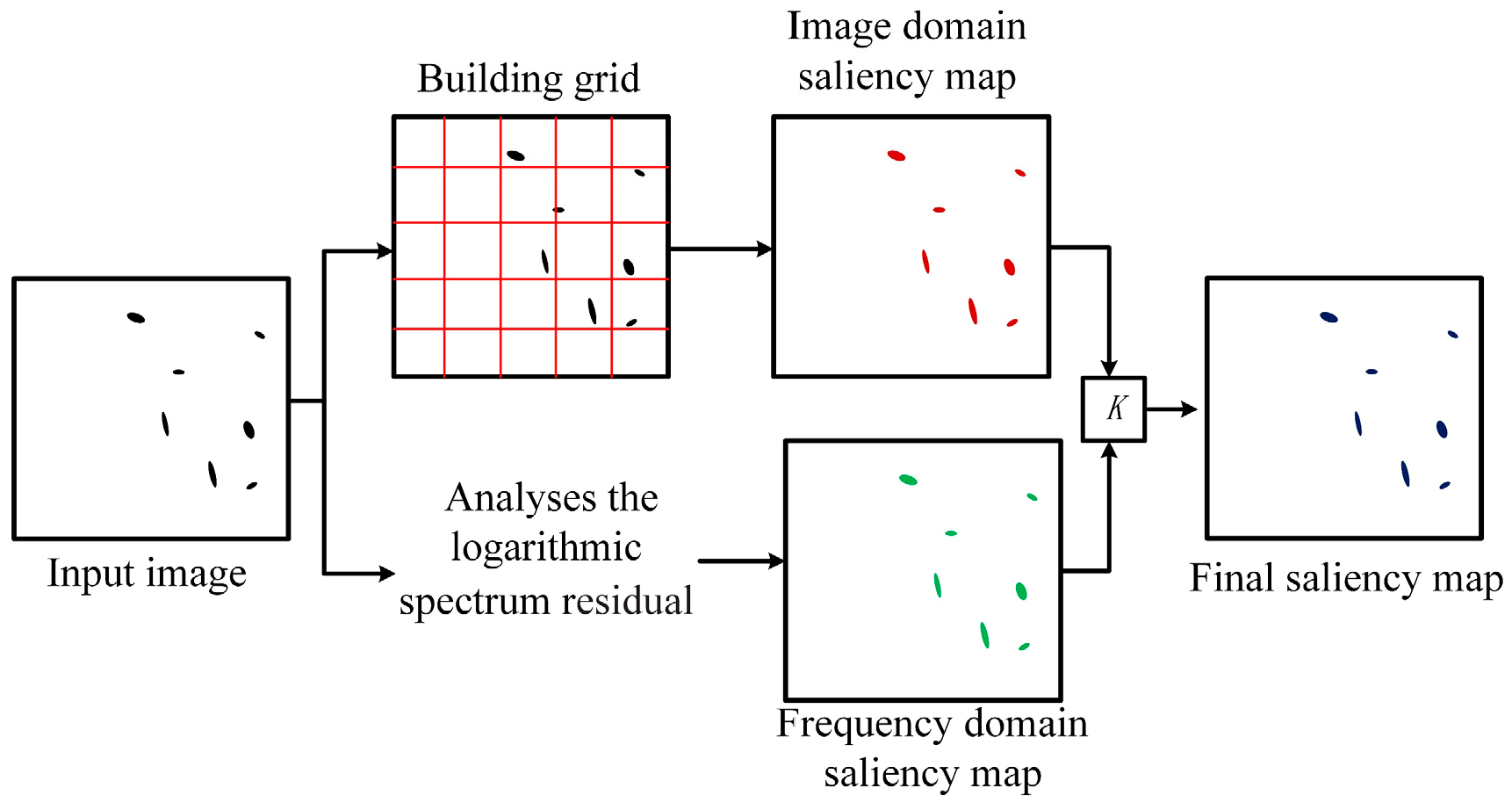
Visual attention mechanism is an image enhancement algorithm that simulates the human eyes, which can quickly focus on ROI [28,29]. Ships are prominent objects in wide maritime areas that human eyes can easily focus on and quickly pick them out. Inspired by this idea, a ship target coarse detection method based on an improved visual attention mechanism is designed in this paper. First, a block-based speed visual attention mechanism is used to suppress the residual area after land–sea segmentation and highlight ship targets, which combines the local intensity feature in image domain with the logarithmic spectrum feature in frequency domain. Then, the mean dichotomy method is adopted to get the coarse detection results of targets adaptively.
The visual attention mechanism proposed in this section can be divided into two branches, the image domain method (an improved version of MSSS [30]) and the frequency domain method, which obtains the saliency image by analyzing the residual information of the logarithmic spectrum in frequency domain. The detailed operations are described in the following sections.
3.2.1. Block-Based Speed Visual Attention Mechanism
The MSSS method is a typical saliency algorithm in the image domain that has the advantages of accuracy and simplicity. It deems that the saliency of the target depends on how it differs from its surrounding environment. The surrounding environment information is extracted by using center surround-filtering [30].
For an input image of width and height , the saliency value at is obtained as:
where is the norm and is the corresponding CIELAB image pixel vector. is the average CIELAB vector of the sub-image whose center pixel is at position , which is given by:
The offsets and area of the sub-image are computed as:
MSSS is a method proposed for optical images and cannot be directly used in single-channel grayscale SAR images. Moreover, the calculation burden caused by the pixel-by-pixel operation is enormous. Therefore, according to the characteristics of SAR images, this paper improves the MSSS method and designs a fast block saliency detection method.
Instead of using the central surround filter, we mesh the image with grids. The grid is set as a square and the size is generally selected as twice the length of the maximum detection ship (for example, for a ship target with maximum 100 pixels, the grid size can be set to 200 pixels). The generated grid region is a schematic illustration. Specifically, if the size of girds is set to be , then every block in the grid can be indexed. For example, the index of the grid block in the third row and the fifth column is .
Input image I, and the saliency value at is obtained by:
where is the intensity value of the pixel at . is the mean of the pixel intensity in the corresponding grid block, which is obtained by:
where and are the width and height of the grid.
Equation (4), as an improvement to Equation (1), is used to measure the difference between two intensity values. Since SAR images are single-channel intensity data, L2 norm can effectively measure the difference between two intensity values. The reason is replaced by is that can achieve better enhancement effect in experiments. Usually ship targets are the highlight area in the SAR image and the intensity of the clutter around is smaller than that of ship targets in a specific range. This is the basis of Equation (4), which is also the theoretical basis of the CFAR detection method. The modified method uses grid blocks to estimate the background, which not only dramatically reduces the computational complexity but also achieves comparable results as the MSSS method. Further, to solve the problem that the intensity value may be discontinuous at the grid boundary, we combine the image domain method with the frequency domain method. Unlike the image domain method that extracts local features, the frequency domain method obtains saliency maps by analyzing the overall features of the image.
The frequency domain saliency method analyses the logarithmic spectrum of the input image and obtains saliency map of the image by extracting the residual spectral information of the image in frequency domain [31].
Specifically, the Fourier transform is performed on the input image, which yields:
where denotes the Fourier transform and A, P, and L represent amplitude, phase, and logarithm, respectively.
Spectral residual can be obtained by:
where is a local average matrix with the size of (n is set to 3 in the experiment) and it can be obtained by:
The saliency map is computed as:
where denotes the inverse Fourier transform and is a Gaussian filter with a standard deviation of 8 [31].
The frequency domain saliency method has a fast processing speed, but the details of targets are still vague. In order to improve the quality of the saliency map effectively, we combine the frequency domain method with the improved image domain method, and the final saliency map is given by:
where the parameter is a weighting factor. With closing to 1, the influence of the image domain saliency map will be greater, which means the details of the image will be clearer. In other words, if the value of approaches 0, the frequency domain saliency map will dominate comparatively, which means the overall characteristics of the target are obvious. Commonly, the value of is 0.6, which can realize a good result in practice. Combining the image domain with the frequency domain saliency method, the detected target is more complete and the speed is much faster than MSSS. The flow chart of the improved visual attention mechanism is show in Figure 1.
3.2.2. Adaptive Threshold Selection
The detection method based on the saliency map usually relies on a pre-defined threshold to realize the transformation from the saliency map to binary detection results. However, this threshold is not robust, which restricts the application of the model in different conditions. For the automatic target detection system of SAR, it is favorable to design an automatic detection method without artificial interference. In this paper, the concept of mean dichotomy in the field of mathematics is introduced into the target rough segmentation step to replace the hard threshold segmentation. The mean dichotomy method solves the threshold by iteration. In each iteration, the mean value of the image is taken as the segmentation threshold to make the image divided into the ship target pixel and the background clutter pixel. In the next iteration, the background clutter pixels are assigned to be the segmentation threshold in the previous round. In this way, the threshold will gradually approximate the ship targets’ intensity.
Supposing the initial image is , the iterative process can be expressed as:
Step 1: Count the statistic of the intensity distribution:
where indicates the number of pixels with intensity .
Step 2: Calculate the mean value:
Step 3: Update the intensity value:
Step 4: If the number of iterations is less than the default value, then go back to Step 1.
The mean dichotomy method makes the threshold value approach the intensity of the high brightness targets in the image by iteration. The updated range of mean value decreases with the increase of the iteration times. In practical applications, the times of the iteration is usually 5 and the mean value in the final iteration is selected as the segmentation threshold. For our method, the convergence speed is analyzed in Appendix A.
3.3. The Fine Detection of Ship Targets Based on Block Kernel Density Estimation
A saliency detection method combining the image domain with the frequency domain is proposed in Section 3.2 and the adaptive threshold selection method is adopted to obtain the coarse detection results of ship targets. The coarse detection results can indicate the ROI but cannot provide accurate contour information. Also, it does not satisfy the CFAR property. In reality, it is not enough to indicate the precise ship targets only by saliency maps. In reference [2], a method using a dynamic constant-false-alarm-rate-based contour saliency model (CSM) to gradually filter out the false alarms from candidate regions and extract the target outlines for accurate detection is proposed. However, it does not apply to the situation where the ship is close to each other. In reference [10], superpixel blocks around the candidate superpixel blocks count clutter information. Yet the use of the superpixel method leads to a large amount of computation and the Gaussian clutter model it uses has a great risk of mismatch. The idea of this section is to take the rough detection results in the previous section as the ship target candidates, then complete the precise detection based on the original SAR image under the criterion of CFAR. Accordingly, this section constructs the BKDE method for ship target precise detection, which consists of two parts: the design of a block detection window and the speed kernel density estimation. Compared with the above method, the proposed BKDE method has low level computation burden and can avoid the influence of target pixels on the clutter distribution statistics. Moreover, its nonparametric estimation characteristic eliminates the mismatch risk of the clutter model.
3.3.1. The Design of the Block Detection Window
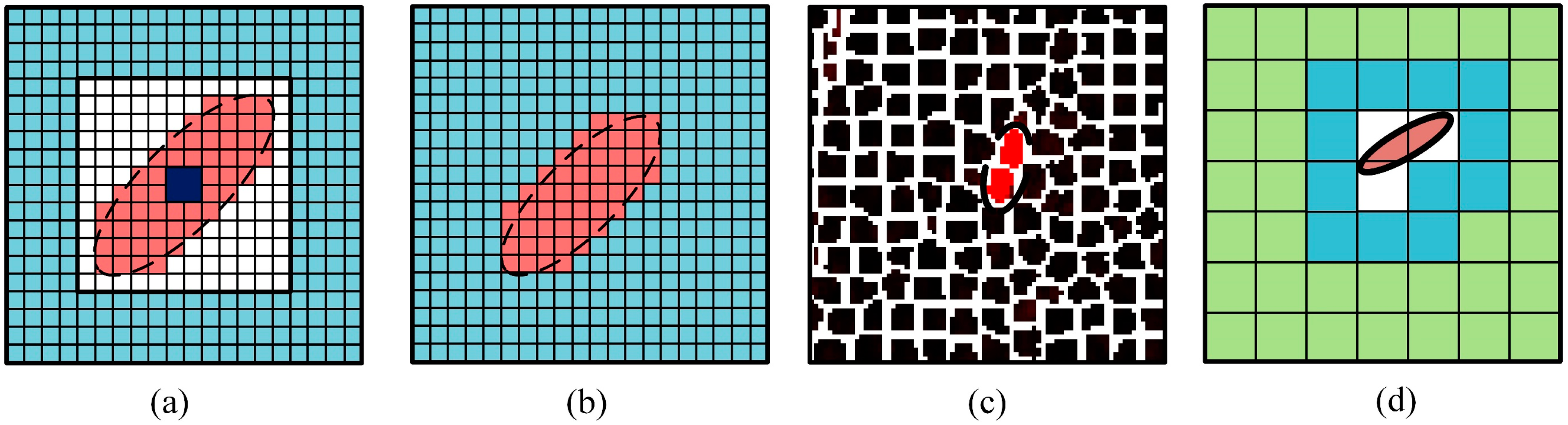
The construction of the detection window in CFAR detector is an important factor affecting the final detection results. The traditional CFAR method estimates the sea clutter parameters by nesting the target window in the background window [4]. As shown in Figure 2a, the blue area, white area, black area, and red area represent background window, protection window, target window, and ship target, respectively. This method may cause the target pixel entering the background window and the degradation of detection results. To solve this problem, the common method is to extract the target candidate region at first and then estimate the clutter parameters with the surrounding pixels of the candidate region [8], as shown in Figure 2b. However, it may also induce a risk that the target may leak into the background window. Another way is to use superpixel segmentation for the target coarse detection, and then select superpixel blocks around its candidate superpixel for the precise detection [9]. As shown in Figure 2c, the red region is the superpixel block where the ship target is located. However, this superpixel segmentation method generates a large amount of computation.
To solve these problems, this section constructs a block detection window. Using the grid blocks in Section 3.2, we remove the grid blocks where the candidate targets are detected. Then, the sea clutter model can be estimated based on the eight neighborhoods of the candidate target grid blocks. The schematic diagram of the block detection window is shown in Figure 2d, where the white blocks are the blocks containing the candidate targets, and the blue blocks are the eight neighborhoods of the candidate target grid blocks.
It should be noted that the block detection window not only avoids the risk that the target pixels leak to the background window affecting the accuracy of the parameter estimation but also effectively avoids the computational pressure caused by superpixel segmentation, which is efficient and effective.
3.3.2. The Speed Kernel Density Estimation
In addition to the design of the detection window, the construction of the sea clutter distribution model and its parameter estimation are also important factors affecting the detection results. To characterize the clutter distribution precisely, researchers have proposed a variety of distribution models. However, when radar parameters change or in complex sea conditions, these clutter models will have a high risk of mismatch. To solve this problem, a nonparametric modeling method is introduced in this paper. Nonparametric density estimation fits the distribution according to the characteristics and properties of the data without prior knowledge, which provides greater flexibility in modeling a given data set. Unlike classical methods, it is not affected by model mismatch [32,33].
Kernel density estimation is one of the effective nonparametric estimations. The basic idea of the kernel density estimation method is to get the estimation of statistical distribution by the weighted sum of kernel functions. The common kernel functions include uniform function, triangle function, cosine function, and Gauss function. In this paper, we choose the standard normal distribution as the kernel function, and its probability density function (PDF) is as follows
The kernel density estimation for SAR images is defined as:
where N is the number of sample points, represents the magnitude of sample pixels and , and controls the smoothness of estimation, which is also known as bandwidth. The performance of the estimation function mainly depends on the selection of in the above formula. In this paper, we choose the method in reference [31] to estimate the optimal window width , namely:
where can be calculate by the pixel amplitude histogram.
Assume that the detection threshold is T and the false alarm probability is given as , then
The detection threshold T can be calculated by the above formula. However, Equation (19) has no analytic solution. In this section, numerical solutions are obtained by approximate calculation [34].
The pixel values in the SAR image are sorted and divided into segments with interval , which can be expressed as . When is selected small enough (generally half of the bandwidth), the cumulative distribution function (CDF) approximates to
Calculate the Equation (20), and when , the detection threshold can be obtained as .
By analyzing the Equations (17) and (20), it is obvious that each calculation of needs to calculate three times of , and each calculation of needs to traverse all the pixels in the image, which undoubtedly brings great computational pressure.
To solve this problem, a frequency domain accelerated calculation method of Gauss kernel density function is proposed. Analyzing the Equation (17), the essence of the component is the weighted sum of the Gaussian distance between x and the sample pixel value at the occurrence frequency. In this section, the frequency weighted form is replaced by the pixel amplitude histogram with interval . Hence, Equation (17) is rewritten as:
where is the pixel amplitude histogram.
Obviously, Equation (21) conforms to the typical discrete convolution expression. The convolution operation in the time domain can be implemented by the frequency domain multiplication, and the Fourier transform has a fast operation approach. Convert Equation (21) into frequency domain to calculate the estimated values of each point through one-time solution, which greatly reduces the amount of calculation. The specific operation is as follows
where .
The computation complexity is analyzed in Appendix B.
In general, the adaptive hierarchical ship detection can be summarized as the following steps:
Step 1: The input SAR image is preprocessed by Otsu method.
Step 2: The improved visual attention mechanism is used to obtain the saliency map of the detected region.
Step 3: Based on the saliency map, the mean dichotomy method is adopted to get the rough detection results of ship targets adaptively.
Step 4: The block detection window is constructed in the neighborhood of the candidate targets.
Step 5: The speed kernel density estimation method is used to obtain the detection threshold and the precise detection results under the concept of CFAR.
Figure 3 shows the flowchart of the proposed ship detection method.
4. Results
To verify the effectiveness of the proposed method, several SAR images are selected for processing. The results are compared with the processing results of various ship detection methods.
4.1. Saliency Algorithm Comparison
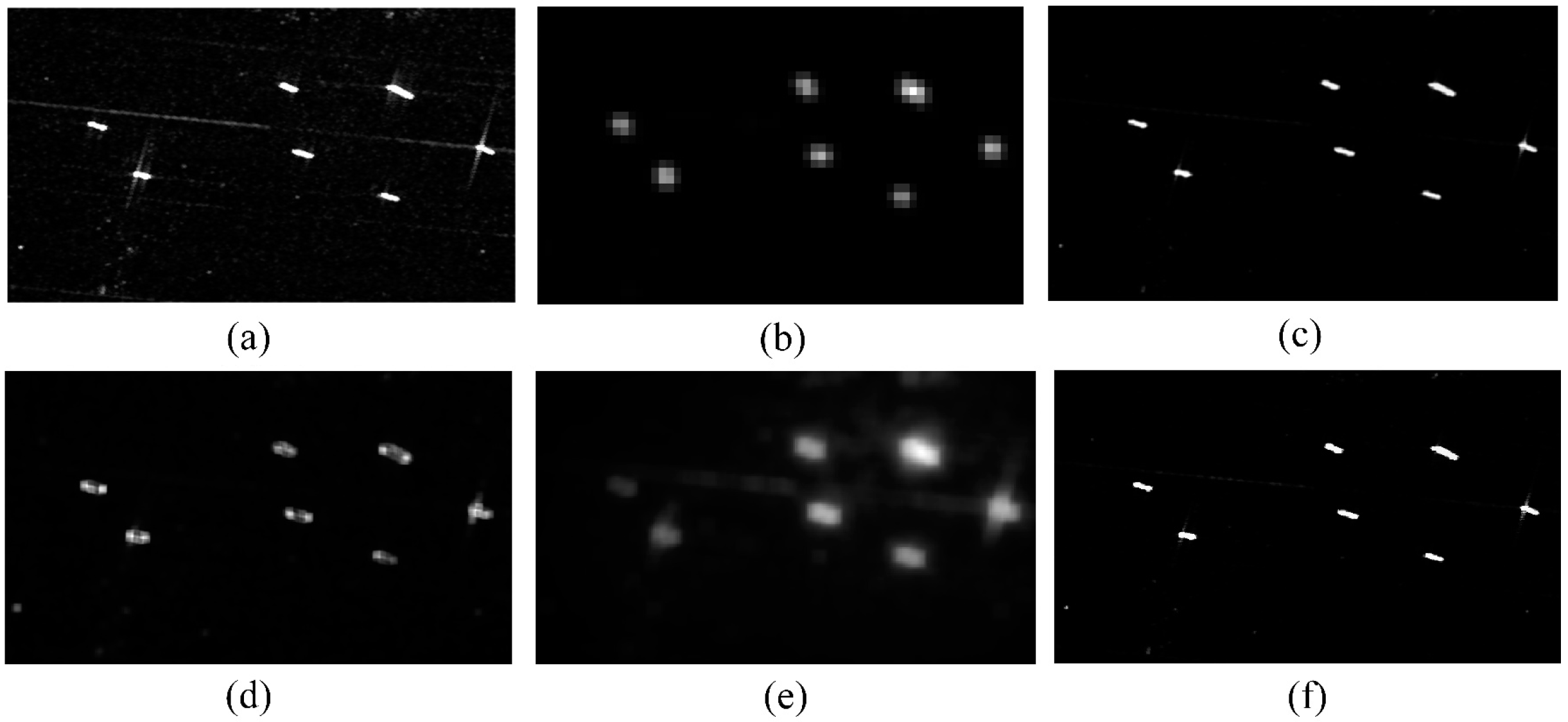
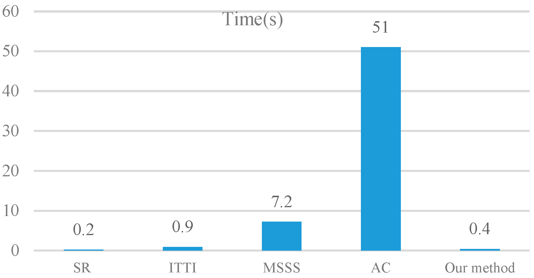
In the experiment, a 3-m-resolution image of RadarSat–2 at the port of Vishakapatnam, India was captured. Based on this picture, the processing results of MSSS [30], AC [35], ITTI [36], and SR [31] are compared with the saliency algorithm proposed in this section. As shown in Figure 4, Figure 4a is the input image, Figure 4b,d,e are the results of ITTI, SR, and AC, respectively, which are fuzzier than the results of MSSS and the proposed method illustrated in Figure 4c,f. The processing time of each saliency algorithm for the image with 1024 1024 pixels is counted in Figure 5, which shows that SR has the shortest computing time and AC has the longest one. The proposed method has the comparable efficiency to SR. Based on the results of Figure 4 and Figure 5, it can be concluded that the saliency method with better image processing performance tends to have a higher calculation load, while the saliency map obtained by the less computation method tends to be fuzzier and loses details. In contrast, considering the characteristics of SAR images, the proposed method has not only clear details but also a less computation load.
4.2. Comparison of Clutter Fitting Performance
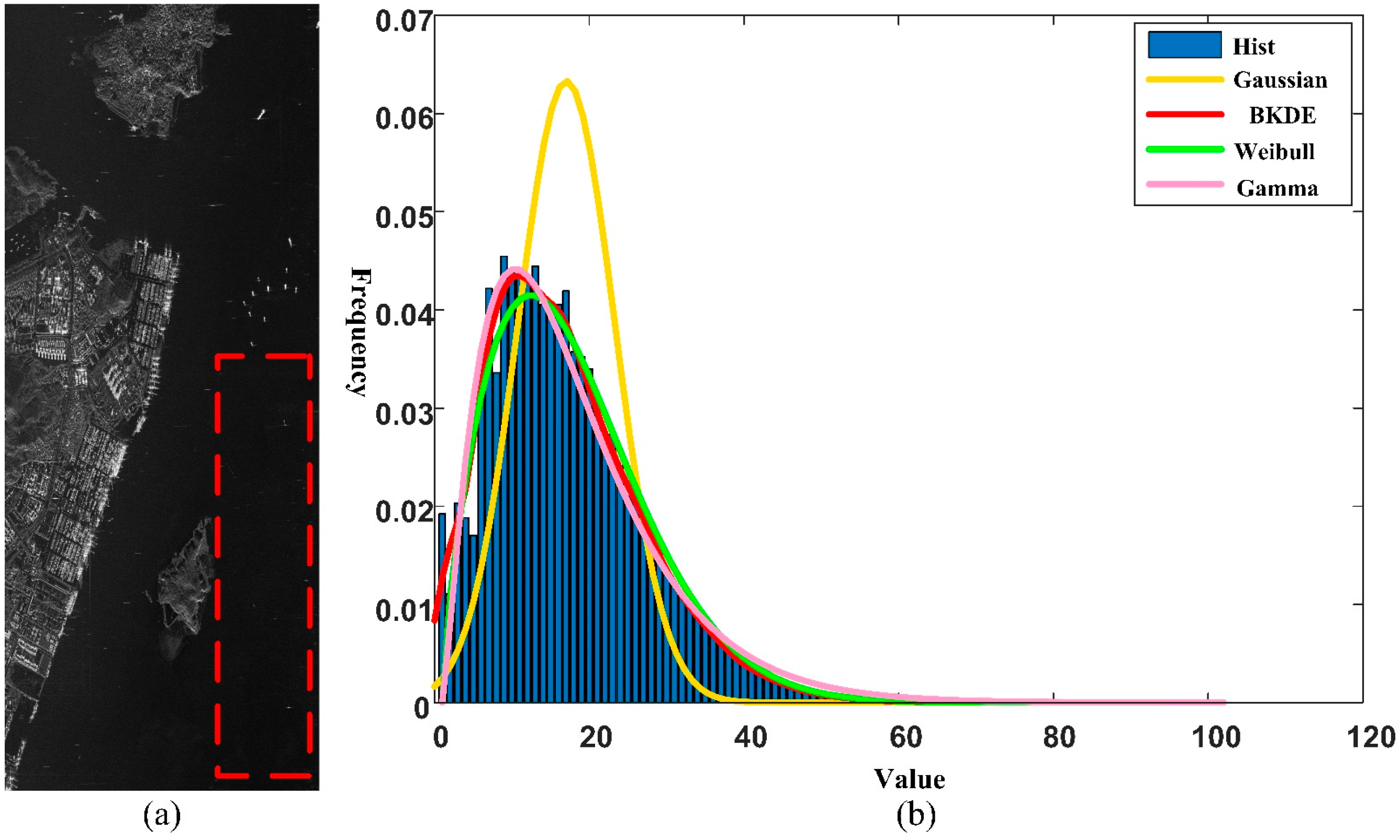
A 1-m-resolution SAR image of a GF-III satellite in Amoy is shown in Figure 6a. The red rectangle marks the range of the clutter area, and its gray distribution histogram is shown in Figure 6b. The fitting results of the Gaussian distribution, the Gamma distribution, the Weibull distribution, and the BKDE on the histogram are also shown in Figure 6b. It can be seen from Figure 6b that the BKDE represented by the red curve has the best fitting performance.
To quantitatively assess the fitting result, we adopt the Kolmogorov–Smirnov (KS) test [37] and Kullback–Leibler (KL) distance [34] as similarity measurements. The KL distance is also called relative entropy. It measures the difference between two probability distributions in the same event space. KS test is the abbreviation of the Kolmogorov-Smirnov test. Unlike other test methods, the distribution model of data is not required for KS test, which is a commonly used nonparametric test method. These two similarity measures have complementary characteristics.
A. KS Test
Suppose there is a set of independently and identically distributed observation samples , which are arranged in ascending order to obtain . The cumulative distribution function (CDF) of the sample data can be expressed as:
The KS statistic is defined as the supremum of the magnitude difference between sample data’s CDF and theoretical CDF. Assuming the theoretical CDF is .
B. KL Distance Measurement
Assuming that the theoretical PDF is , and the actual PDF is , then the KL distance between two densities and is:
The approximate calculation value is:
where is the theoretical probability distribution histogram, is the actual probability distribution histogram, and represents the sample space. Because is not symmetrical, i.e., the symmetric KL distance can be expressed as:
KL distance represents the similarity between the two distributions. When the actual distribution is the same as the theoretical distribution, the KL distance is zero. Unlike KL distance, KS describes the cumulative distribution function (CDF) gap between two distributions. KS test will be smaller with the decrease of the difference between the two CDFs. Figure 7 shows the fitting performance of each distribution in Figure 6 and it demonstrates that the BKDE method has better a fitting performance. The reason is that the Gaussian distribution, the Gamma distribution, and the Weibull distribution are all specific models for different sea conditions. When sea conditions change, there will be a risk of mismatch. As a nonparametric model estimation method, BKDE can keep a robust fitting effect when the environment changes.
4.3. Comparison of the Ship Target Detection Performance
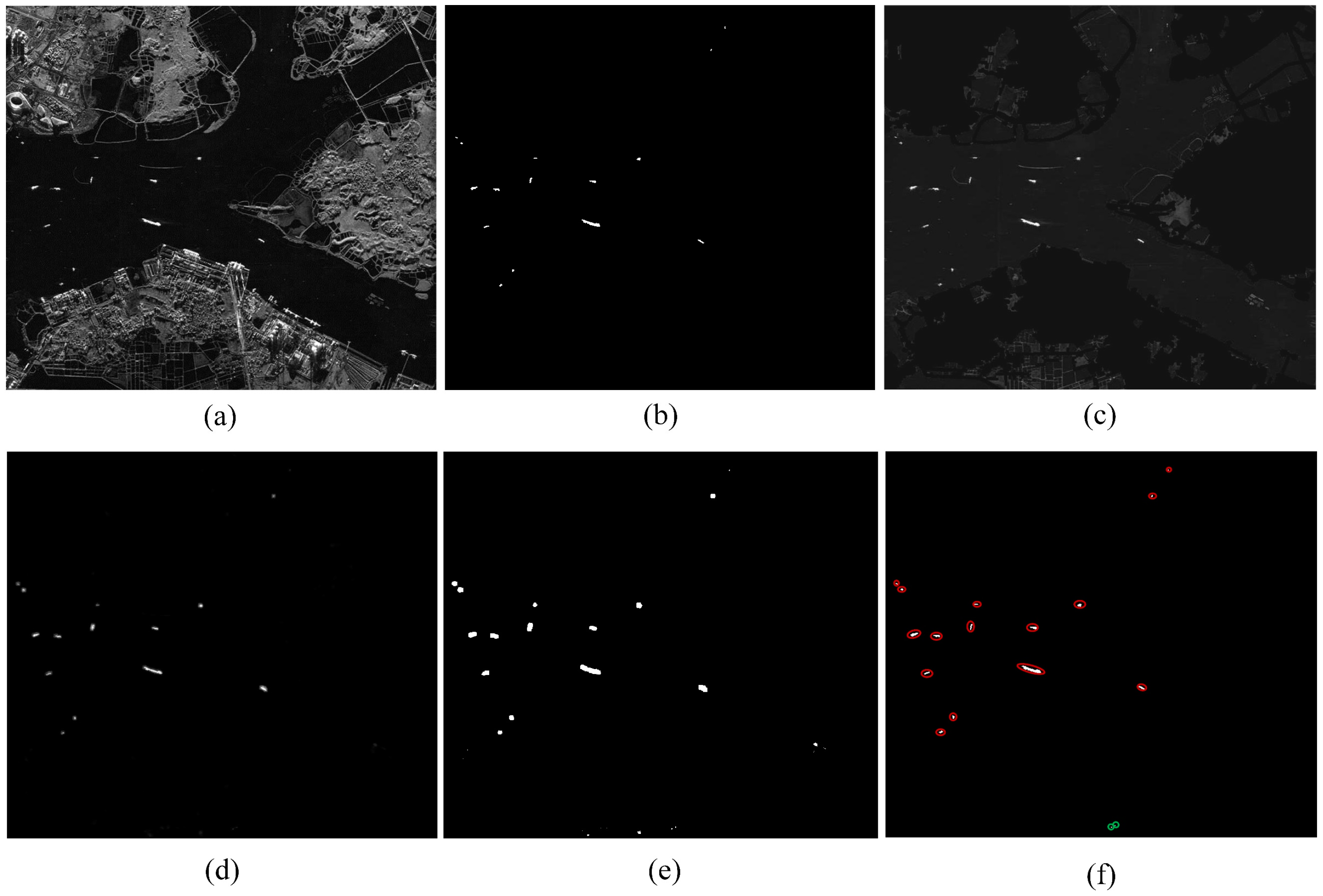
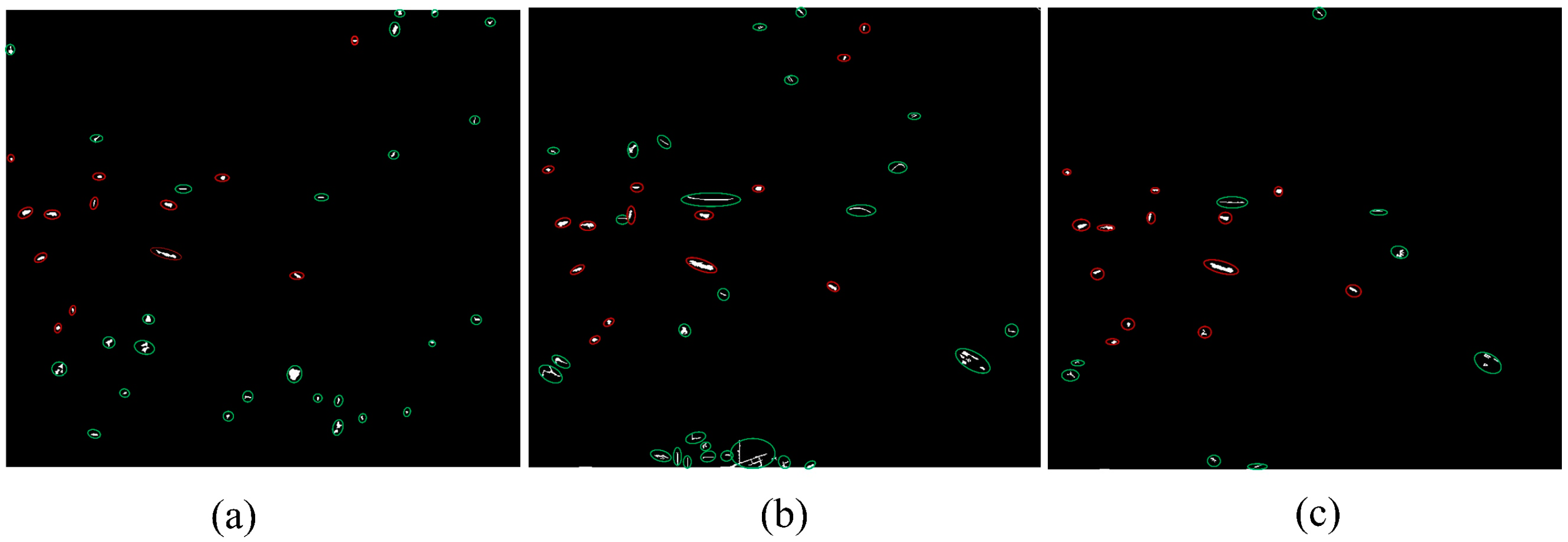
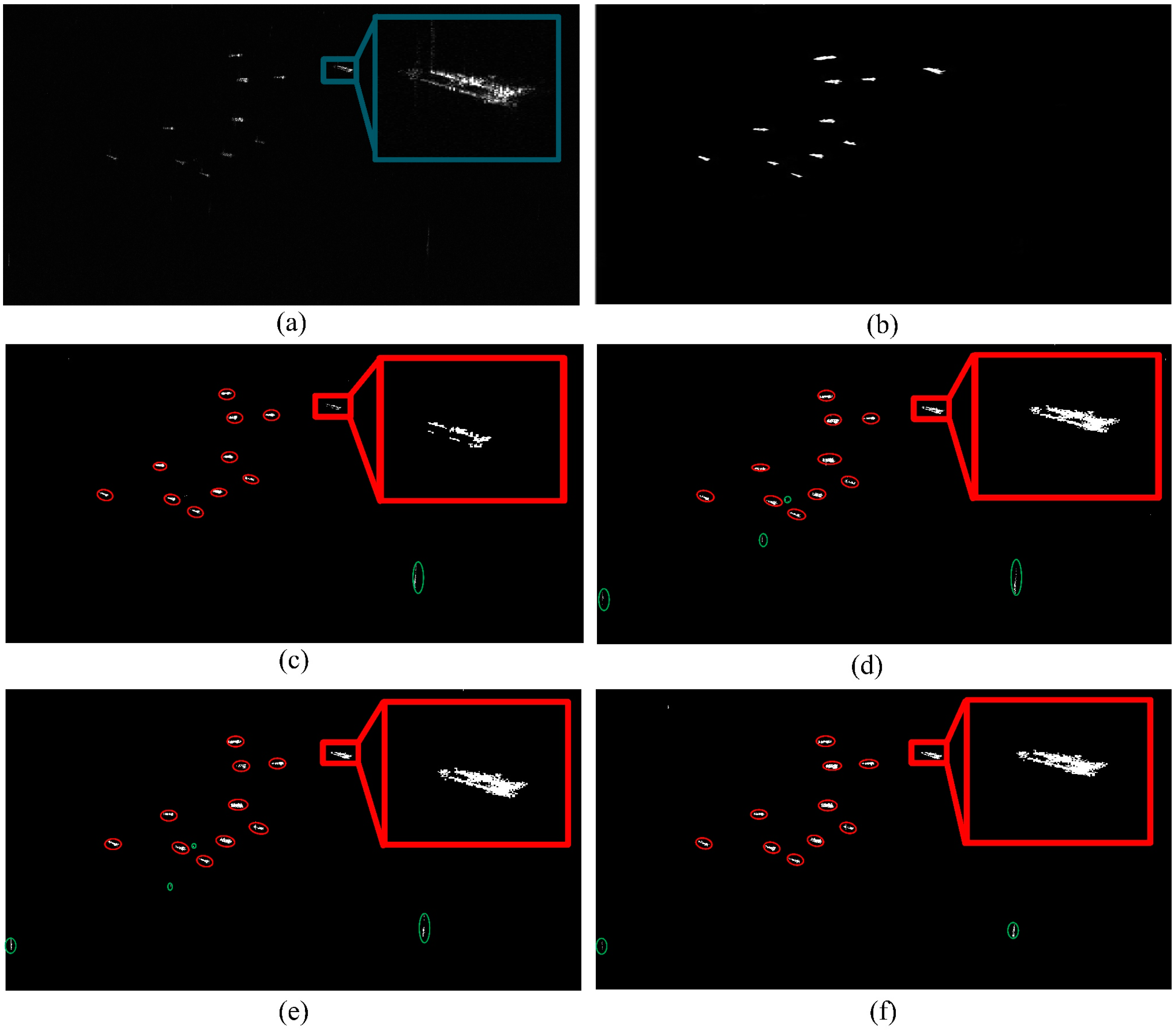
When land exists in the detection area, land–sea segmentation is a necessary operation. In the experiment, we find that when using Otsu for land–sea segmentation, the near-shore area is difficult to remove due to the low reflection intensity, and there are still many residual areas after the segmentation, which seriously affect the later detection stage. In SAR images, the intensity of the near-shore area is higher than that of the land area and smaller than that of the sea area, so it cannot be clearly divided into the two sets. That is the inherent defect of the Otsu. The proposed improved saliency method can effectively suppress the residual area, as shown in Figure 8. Figure 8a is a 1.5-m-resolution airborne SAR image with size 790 709 pixels. Figure 8b is the ground truth that is created by combining prior information with photointerpretation based on the input image Figure 8a. The ground truth generation method introduced in [28] and [2] is adopted. Figure 8c–f show the results of land–sea segmentation, saliency map, rough detection and fine detection under the false alarm rate , respectively. The red ellipses and green ellipses in the figures represent the correct and false test results, respectively. (The red and green ellipses are drawn on the basis of the detection results, which is used to enhance the display effect of the results) Figure 9a–c show the detection results of two-parameter method [4], multiscale method [8], and superpixel method [10] under false alarm rate . Compared with the detection result of the proposed method shown in Figure 8f, more false alarm targets are detected by the comparison methods.
For pure sea background, land–sea segmentation can be avoided. A 1-m-resolution SAR image of GF-III satellite with the size of pixels is shown in Figure 10a. Figure 10b is the ground truth. The data comes from the open dataset published in the Journal of Radars [38]. The difficulty in detecting is that its detection scene is relatively large. Because of the high resolution of the image, it is crucial that whether the detection method can retain the details of the target. The detection results of two-parameter method, multiscale method, superpixel method and the proposed method under the false alarm rate are presented in Figure 10c–f. As shown in Figure 10c, the result of two-parameter CFAR shows it loses a quantity of target pixels. Moreover, Figure 10d–f shows that the multiscale method, the superpixel method, and the proposed method can preserve the target details well.
In addition to quantitatively analyzing the detection performance of each method, we used detection rate and false alarm rate to evaluate the performance of each detection method, which are also used in [2,9]. Suppose the number of the target pixel in the image is , the correct detected target pixels is . The detection rate is defined as:
False alarm rate is defined as [8,9]:
where is the number of clutter pixels in the SAR image, and is the number of clutter pixels which are detected as target pixels a good ship detector should keep the balance between the detection rate and the false alarm rate.
Table 1 counts the detection results of each detection method of Figure 8a and Figure 10a, and gives the comparison of detection rate, false alarm rate and detection time. The comparison results in Table 1 are consistent with those shown in the figures above. From the table it can be seen the proposed method has a higher detection rate and a lower false alarm rate. Moreover, it also indicates that our method has better performance than its counterparts in terms of the detection efficiency.
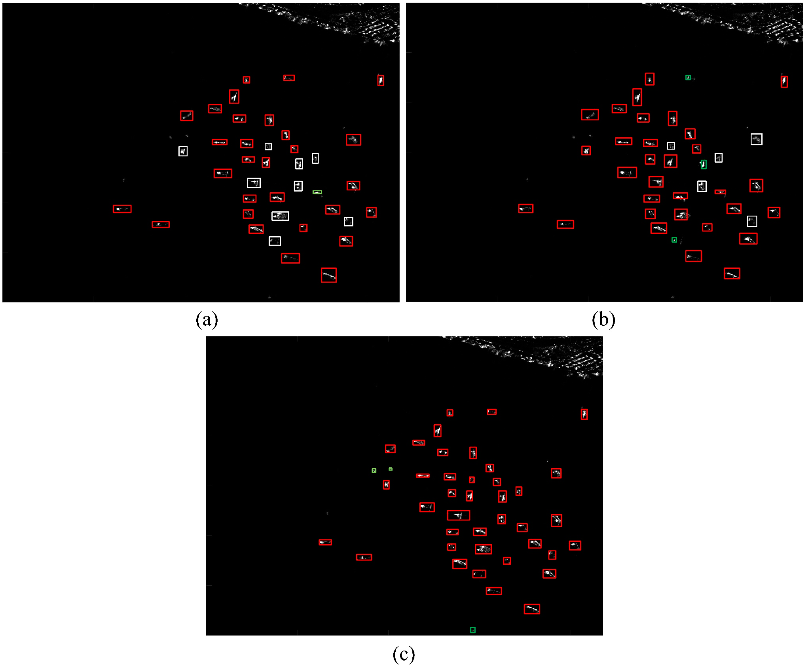
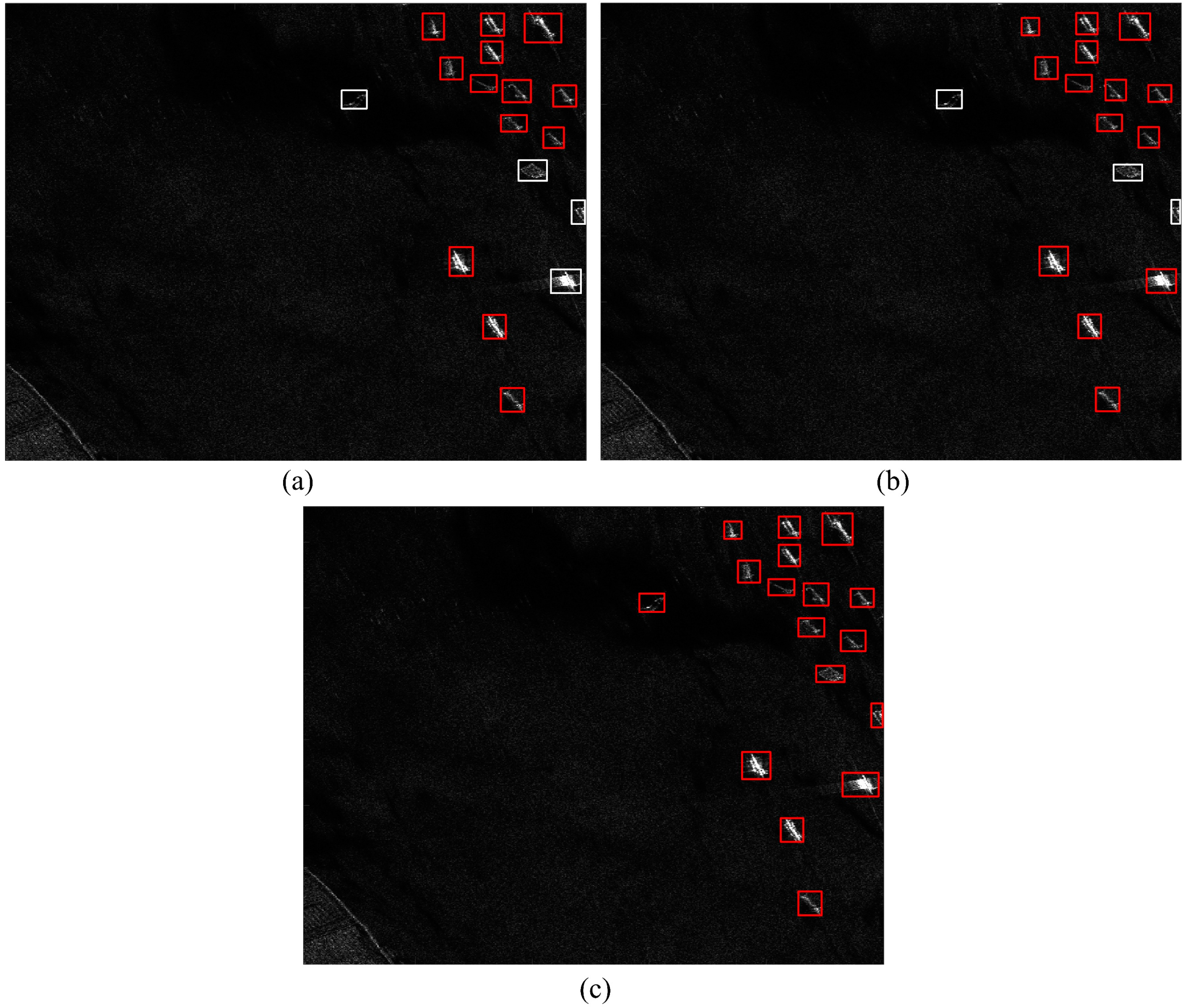
In the above experiment, the detection results of the proposed algorithm are compared with algorithms under the concept of CFAR. The following experiment is used to compare the detection results of the proposed algorithm and deep learning methods. SAR ship detection dataset (SSDD) [39] is used in the training of models. The dataset contains 1160 SAR images and 2456 ships. Figure 11 and Figure 12 shows the detection and comparison results of Yolo_v3 [21], densely-faster-RCNN [3], and the proposed method. Figure 11 and Figure 12 are the open dataset published in the Journal of Radars [38], which has SAR images and their ground truths.
Consider the peculiarity of learning method, we apply the evaluation criteria mentioned below to evaluate the quality of the method, which are also used in [3,14]. The target detection accuracy is defined as:
Recall is defined as [3,14]:
where is the number of correct detected objects, denotes the number of detected ships, is the number of ground-truth. Table 2 displays the performance of three methods.
Figure 11 and Figure 12, and Table 2 show that comparing with the deep learning method the proposed method has higher a recall rate. The deep learning methods have a low recall rate because the SAR imaging results defocus when the ship target moves and if the data set does not contain this case the method cannot detection the target. Besides, the reason for the proposed method has lower detection accuracy is that it detects ships based on the intensity of the pixel, which may lead to some bright spots on the sea being detected as target ships. With the guarantee that the targets are all detected, these false alarms can be removed by subsequent discrimination operations, i.e., eigenellipse discrimination or maximum-likelihood (ML) discrimination [8].
5. Conclusions
In order to improve the robustness of ship target detection in high-resolution SAR and avoid the mismatch risk of the clutter model, a nonparametric fast high-resolution SAR image ship target detection method based on the coarse-to-fine mechanism is proposed in this paper. First, an improved visual attention mechanism combining the image domain with the frequency domain is constructed. It not only produces a saliency map that maintains better image details, but also has a higher speed than other attention mechanisms. Then, the candidate target region segmentation threshold is obtained by the mean dichotomy, which eliminates the instability caused by the hard threshold selection. Third, the speed block kernel density estimation method is used to perform ship target precise detection. The idea of region partitioning avoids the computational burden of superpixel segmentation and the kernel density estimation eliminates the mismatch risk of the clutter model. In addition, the frequency domain acceleration method improves the execution efficiency of the detection method. Compared with existing ship target detection methods in high-resolution SAR images, the proposed method can detect the target while maintaining the CFAR characteristics. Experiments and data processing verify the effectiveness of the method.
Author Contributions
Conceptualization, Y.L.; methodology, Y.L., and K.S.; writing—original draft preparation, Y.L., K.S., Y.Z., G.L., and M.X. All authors have read and agreed to the published version of the manuscript.
Funding
This work was supported by the National Natural Science Foundation of China under Grant 61971326.
Acknowledgments
The authors would like to thank the anonymous reviewers for their valuable comments to improve the paper quality.
Conflicts of Interest
The authors declare no conflict of interest.
Appendix A
This part is to analyze the convergence speed of the mean dichotomy method. It should be noted that the convergence speed at the initial iteration stage is hard to analyze because it relates to the ratio of target to clutter pixel and the clutter distribution model. However, when the iteration goes into later stages, the process can be simplified to the following form:
where and are the intensity of clutter pixels and ship pixels, respectively. The reason for this simplification is that the pixel intensity of the ship target is often higher than that of the sea clutter. Then, Equation (14) can be rewritten as:
Calculate the derivative of , we have:
Since ,
Then:
Hence, the threshold value obtained by the iteration gradually increases. Meanwhile,
Therefore, the convergence speed of threshold gradually decreases.
Appendix B
This part is to analyze the computation complexity of speed KDE. The calculation burden comes from the following equation:
If one real addition or one real multiplication is regarded as one operation, FFT or IFFT needs operations ( is the number of FFT operation). So, the computation complexity of Equation (A8) is proportional to .
The computation complexity of the original KDE method mainly comes from:
Equation (A9) needs almost operations (N is the number of sample points). Generally, the pixel number for estimating the clutter distribution is selected as , and the value is selected as 1000. So . The computation complexity of speed KDE is obviously less than that of original KDE.
References
- Philippe, S.; Sergi, L.; Carlos, L. Ship Detection in SAR Images Based on Maxtree Representation and Graph Signal Processing. IEEE Trans. Geosci. Remote Sens. 2019, 57, 2709–2724. [Google Scholar]
- Wang, S.; Wang, M.; Yang, S.; Jiao, L. New hierarchical saliency filtering for fast ship detection in high-resolution SAR images. IEEE Trans. Geosci. Remote Sens. 2017, 55, 351–362. [Google Scholar] [CrossRef]
- Jiao, J.; Zhang, Y.; Sun, H.; Yang, X.; Gao, X.; Hong, W.; Fu, K.; Sun, X. A Densely Connected End-to-End Neural Network for Multiscale and Multiscene SAR Ship Detection. IEEE Access 2018, 6, 20881–20892. [Google Scholar] [CrossRef]
- Goldstein, G. False-Alarm Regulation in Log-Normal and Weibull Clutter. IEEE Trans. Aerosp. Electron. Syst. 1973, AES–9, 84–92. [Google Scholar] [CrossRef]
- Blake, S. OS-CFAR theory for multiple targets and nonuniform clutter. IEEE Trans. Aerosp. Electron. Syst. 1988, 24, 785–790. [Google Scholar] [CrossRef]
- Schwegmann, C.P.; Kleynhans, W.; Salmon, B.P. Manifold Adaptation for Constant False Alarm Rate Ship Detection in South African Oceans. IEEE J. Sel. Top. Appl. Earth Obs. Remote Sens. 2015, 8, 1–9. [Google Scholar] [CrossRef] [Green Version]
- Leng, X.; Ji, K.; Fan, Q.; Zhou, S.; Zou, H. A novel adaptive ship detection method for spaceborne SAR imagery. In Proceedings of the 2016 IEEE International Geoscience and Remote Sensing Symposium (IGARSS), Beijing, China, 10–15 July 2016; pp. 108–111. [Google Scholar]
- Ao, W.; Xu, F.; Li, Y.; Wang, H. Detection and Discrimination of Ship Targets in Complex Background From Spaceborne ALOS-2 SAR Images. IEEE J. Sel. Top. Appl. Earth Obs. Remote Sens. 2018, 11, 536–550. [Google Scholar] [CrossRef]
- Yu, W.; Wang, Y.; Liu, H.; He, J. Superpixel-Based CFAR Target Detection for High-Resolution SAR Images. IEEE Geosci. Remote Sens. Lett. 2016, 13, 730–734. [Google Scholar] [CrossRef]
- Li, T.; Liu, Z.; Xie, R.; Ran, L. An improved superpixel-level CFAR detection method for ship targets in high-resolution SAR images. IEEE J. Sel. Top. Appl. Earth Obs. Remote Sens. 2018, 11, 184–194. [Google Scholar] [CrossRef]
- Migliaccio, M.; Nunziata, F.; Montuori, A.; Paes, R. Single-look complex COSMO-SkyMed SAR data to observe metallic targets at sea. IEEE J. Sel. Top. Appl. Earth Obs. Remote Sens. 2012, 5, 893–901. [Google Scholar] [CrossRef]
- Almalki, S.J.; Yuan, J. A new modified Weibull distribution. Reliab. Eng. Syst. Saf. 2012, 111, 164–170. [Google Scholar] [CrossRef]
- Qin, X.; Zhou, S.; Zou, H.; Gao, G. A CFAR detection algorithm for generalized gamma distributed background in high resolution SAR images. IEEE Geosci. Remote Sens. Lett. 2013, 10, 806–810. [Google Scholar]
- Lin, Z.; Ji, K.; Leng, X.; Kuang, G. Squeeze and Excitation Rank Faster R-CNN for Ship Detection in SAR Images. IEEE Geosci. Remote Sens. Lett. 2019, 16, 751–755. [Google Scholar] [CrossRef]
- Gao, G.; Liu, L.; Zhao, L.; Shi, G.; Kuang, G. An adaptive and fast CFAR algorithm based on automatic censoring for target detection in high-resolution SAR images. IEEE Trans. Geosci. Remote Sens. 2009, 47, 1685–1697. [Google Scholar] [CrossRef]
- Gao, G.; Shi, G. CFAR Ship Detection in Nonhomogeneous Sea Clutter Using Polarimetric SAR Data Based on the Notch Filter. IEEE Trans. Geosci. Remote Sens. 2017, 55, 4811–4824. [Google Scholar] [CrossRef]
- Di Simone, A.; Iodice, A.; Riccio, D.; Camps, A.; Park, H. GNSS-R: A useful tool for sea target detection in near real-time. In Proceedings of the 2017 IEEE 3rd International Forum on Research and Technologies for Society and Industry-Innovation to Shape the Future for Society and Industry (RTSI), Modena, Italy, 11–13 September 2017. [Google Scholar]
- Reggiannini, M.; Righi, M.; Tampucci, M.; Duca, A.L.; Bacciu, C.; Bedini, L.; D’Errico, A.; Di Paola, C.; Marchetti, A.; Martinelli, M.; et al. Remote Sensing for Maritime Prompt Monitoring. J. Mar. Sci. Eng. 2019, 7, 202. [Google Scholar] [CrossRef] [Green Version]
- Redmon, J.; Divvala, S.; Girshick, R.; Farhadi, A. You Only Look Once: Unified, Real-Time Object Detection. In Proceedings of the 2016 IEEE Conference on Computer Vision and Pattern Recognition (CVPR), Las Vegas, NV, USA, 26 June–1 July 2016; pp. 779–788. [Google Scholar]
- Redmon, J.; Farhadi, A. YOLO9000: Better, Faster, Stronger. In Proceedings of the 2017 IEEE Conference on Computer Vision and Pattern Recognition (CVPR), Honolulu, HI, USA, 21–26 July 2017; pp. 6517–6525. [Google Scholar]
- Redmon, J.; Farhadi, A. Yolov3: An incremental improvement. arXiv 2018, arXiv:1804.02767. [Google Scholar]
- Girshick, R.; Donahue, J.; Darrell, T.; Malik, J.; Malik, J. Rich Feature Hierarchies for Accurate Object Detection and Semantic Segmentation. In Proceedings of the 2014 IEEE Conference on Computer Vision and Pattern Recognition, Columbus, OH, USA, 24–27 June 2014; pp. 580–587. [Google Scholar]
- Girshick, R. Fast R-CNN. In Proceedings of the 2015 IEEE International Conference on Computer Vision (ICCV), Santiago, Chile, 11–18 December 2015; pp. 1440–1448. [Google Scholar]
- Ren, S.; He, K.; Girshick, R. Faster r-cnn: Towards real-time object detection with region proposal networks. IEEE Trans. Pattern Anal. Mach. Intell. 2017, 39, 1137–1149. [Google Scholar] [CrossRef] [Green Version]
- Crisp, D.J. The State-of-the-Art in Ship Detection in Synthetic Aperture Radar Imagery; DSTO-RR–0272; DSTO Information Sciences Laboratory: Edinburgh, Australia, 2004. [Google Scholar]
- Ren, H.; Lv, C.; Zou, F. An improved algorithm for active contour extraction based on greedy snake. In Proceedings of the 2015 IEEE/ACIS 14th International Conference on Computer and Information Science (ICIS), Las Vegas, NV, USA, 28 June–1 July 2015. [Google Scholar]
- Otsu, N. A Threshold Selection Method from Gray-Level Histograms. IEEE Trans. Syst. Man, Cybern. 1979, 9, 62–66. [Google Scholar] [CrossRef] [Green Version]
- Hou, B.; Chen, X.Z.; Jiao, L.C. Multilayer CFAR detection of ship targets in very high resolution SAR images. IEEE Geosci. Remote Sens. Lett. 2015, 12, 811–815. [Google Scholar]
- Gao, L.; Bi, F.; Yang, J. Visual attention based model for target detection in large-field images. J. Syst. Eng. Electron. 2011, 22, 150–156. [Google Scholar] [CrossRef]
- Achanta, R.; Susstrunk, S. Saliency detection using maximum symmetric surround. In Proceedings of the 2010 IEEE International Conference on Image Processing, Hong Kong, China, 26–29 September 2010; pp. 2653–2656. [Google Scholar]
- Hou, X.; Zhang, L. Saliency Detection: A Spectral Residual Approach. In Proceedings of the 2007 IEEE Conference on Computer Vision and Pattern Recognition, Minneapolis, MN, USA, 17–22 June 2007; pp. 1–8. [Google Scholar]
- Botev, Z.I.; Grotowski, J.F.; Kroese, D.P. Kernel density estimation via diffusion. Ann. Stat. 2010, 38, 2916–2957. [Google Scholar] [CrossRef] [Green Version]
- Cui, Y.; Yang, J.; Yamaguchi, Y.; Singh, G.; Park, S.; Kobayashi, H. On semiparametric clutter estimation for ship detection in synthetic aperture radar images. IEEE Trans. Geosci. Remote Sens. 2013, 51, 3170–3180. [Google Scholar] [CrossRef]
- Gao, G. A Parzen-Window-Kernel-Based CFAR Algorithm for Ship Detection in SAR Images. IEEE Geosci. Remote Sens. Lett. 2011, 8, 557–561. [Google Scholar] [CrossRef]
- Achanta, R.; Estrada, F.; Wils, P.; Süsstrunk, S. Salient Region Detection and Segmentation. In Computer Vision—ECCV 2012; Springer: Berlin/Heidelberg, Germany, 2008; Volume 5008, pp. 66–75. [Google Scholar]
- Itti, L.; Koch, C.; Niebur, E. A model of saliency-based visual attention for rapid scene analysis. IEEE Trans. Pattern Anal. Mach. Intell. 1980, 20, 1254–1259. [Google Scholar] [CrossRef] [Green Version]
- Devore, M.D.; A O’Sullivan, J. Quantitative statistical assessment of conditional models for synthetic aperture radar. IEEE Trans. Image Process. 2004, 13, 113–125. [Google Scholar] [CrossRef] [Green Version]
- Xian, S.; Zhirui, W.; Yuanrui, S. AIR-SARShip–1.0: High Resolution SAR Ship Detection Dataset. J. Radars 2019, 8. [Google Scholar] [CrossRef]
- Li, J.; Qu, C.; Shao, J. Ship detection in SAR images based on an improved faster R-CNN. In Proceedings of the 2017 SAR in Big Data Era: Models, Methods and Applications (BIGSARDATA), Beijing, China, 13–14 November 2017; pp. 1–6. [Google Scholar]
Figure 1.
The flow chart of the improved visual attention mechanism.

Figure 2.
The detection windows. (a) Two-parameter constant false alarm rate (CFAR) window. (b) Candidate region window. (c) Superpixel window. (d) Block detection window.
Figure 2.
The detection windows. (a) Two-parameter constant false alarm rate (CFAR) window. (b) Candidate region window. (c) Superpixel window. (d) Block detection window.

Figure 3.
Pipeline of the proposed ship detection method.

Figure 4.
Comparison of saliency algorithm results. (a) Input image. (b) ITTI. (c) MSSS. (d) SR. (e) AC. (f) The proposed method.
Figure 4.
Comparison of saliency algorithm results. (a) Input image. (b) ITTI. (c) MSSS. (d) SR. (e) AC. (f) The proposed method.

Figure 5.
Algorithm processing time.

Figure 6.
Comparison of clutter fitting result. (a) Clutter region. (b) Histogram fitting results.

Figure 7.
Comparison of clutter fitting result.

Figure 8.
The detection results. (a) Input image. (b) Ground truth. (c) Otsu result. (d) Saliency map. (e) Coarse detection result. (f) Fine detection result. The red ellipses and green ellipses in the figures represent the correct and false test results respectively.
Figure 8.
The detection results. (a) Input image. (b) Ground truth. (c) Otsu result. (d) Saliency map. (e) Coarse detection result. (f) Fine detection result. The red ellipses and green ellipses in the figures represent the correct and false test results respectively.

Figure 9.
The detection results. (a) Two-parameter method. (b) Multiscale method. (c) Superpixel method. The red ellipses and green ellipses in the figures represent the correct and false test results respectively.
Figure 9.
The detection results. (a) Two-parameter method. (b) Multiscale method. (c) Superpixel method. The red ellipses and green ellipses in the figures represent the correct and false test results respectively.

Figure 10.
The detection results. (a) Input image. (b) Ground truth (c) Two-parameter method. (d) Multiscale method. (e) Superpixel method. (f) Proposed method.
Figure 10.
The detection results. (a) Input image. (b) Ground truth (c) Two-parameter method. (d) Multiscale method. (e) Superpixel method. (f) Proposed method.

Figure 11.
The detection results. (a) Yolo_v3 result. (b) Densely-faster-RCNN result. (c) Proposed method. The red, white, and green rectangles represent the correct detection ships, the missing ships, and the false alarms, respectively.
Figure 11.
The detection results. (a) Yolo_v3 result. (b) Densely-faster-RCNN result. (c) Proposed method. The red, white, and green rectangles represent the correct detection ships, the missing ships, and the false alarms, respectively.

Figure 12.
The detection results. (a) Yolo_v3 result. (b) Densely-faster-RCNN result. (c) Proposed method. The red, white, and green rectangles represent the correct detection ships, the missing ships, and the false alarms, respectively.
Figure 12.
The detection results. (a) Yolo_v3 result. (b) Densely-faster-RCNN result. (c) Proposed method. The red, white, and green rectangles represent the correct detection ships, the missing ships, and the false alarms, respectively.


Table 1.
Detection performance comparisons ().
| Methods | Time (s) | |||
|---|---|---|---|---|
| Figure 8a | Two-parameter method | 95.3 | 0.89 | 6.8 |
| Multiscale method | 98.1 | 0.86 | 5.3 | |
| Superpixel method | 98.5 | 0.57 | 19.7 | |
| Proposed method | 98.6 | 0.11 | 3.8 | |
| Figure 10a | Two-parameter method | 89.8 | 0.21 | 3007.2 |
| Multiscale method | 91.3 | 0.38 | 11.7 | |
| Superpixel method | 92.4 | 0.34 | 148.7 | |
| Proposed method | 92.7 | 0.24 | 5.3 |
© 2020 by the authors. Licensee MDPI, Basel, Switzerland. This article is an open access article distributed under the terms and conditions of the Creative Commons Attribution (CC BY) license (http://creativecommons.org/licenses/by/4.0/).
Share and Cite
MDPI and ACS Style
Liang, Y.; Sun, K.; Zeng, Y.; Li, G.; Xing, M. An Adaptive Hierarchical Detection Method for Ship Targets in High-Resolution SAR Images. Remote Sens. 2020, 12, 303. https://0-doi-org.brum.beds.ac.uk/10.3390/rs12020303
AMA Style
Liang Y, Sun K, Zeng Y, Li G, Xing M. An Adaptive Hierarchical Detection Method for Ship Targets in High-Resolution SAR Images. Remote Sensing. 2020; 12(2):303. https://0-doi-org.brum.beds.ac.uk/10.3390/rs12020303
Chicago/Turabian StyleLiang, Yi, Kun Sun, Yugui Zeng, Guofei Li, and Mengdao Xing. 2020. "An Adaptive Hierarchical Detection Method for Ship Targets in High-Resolution SAR Images" Remote Sensing 12, no. 2: 303. https://0-doi-org.brum.beds.ac.uk/10.3390/rs12020303
Note that from the first issue of 2016, this journal uses article numbers instead of page numbers. See further details here.