Measuring the Directional Ocean Spectrum from Simulated Bistatic HF Radar Data


1
School of Mathematics and Statistics, University of Sheffield, Sheffield S10 2TN, UK
2
Seaview Sensing Ltd., Sheffield S10 3GR, UK
*
Author to whom correspondence should be addressed.
†
These authors contributed equally to this work.
Remote Sens. 2020, 12(2), 313; https://0-doi-org.brum.beds.ac.uk/10.3390/rs12020313
Submission received: 19 December 2019
/
Revised: 9 January 2020
/
Accepted: 14 January 2020
/
Published: 18 January 2020
(This article belongs to the Special Issue Bistatic HF Radar)
Abstract
:HF radars are becoming important components of coastal operational monitoring systems particularly for currents and mostly using monostatic radar systems where the transmit and receive antennas are colocated. A bistatic configuration, where the transmit antenna is separated from the receive antennas, offers some advantages and has been used for current measurement. Currents are measured using the Doppler shift from ocean waves which are Bragg-matched to the radio signal. Obtaining a wave measurement is more complicated. In this paper, the theoretical basis for bistatic wave measurement with a phased-array HF radar is reviewed and clarified. Simulations of monostatic and bistatic radar data have been made using wave models and wave spectral data. The Seaview monostatic inversion method for waves, currents and winds has been modified to allow for a bistatic configuration and has been applied to the simulated data for two receive sites. Comparisons of current and wave parameters and of wave spectra are presented. The results are encouraging, although the monostatic results are more accurate. Large bistatic angles seem to reduce the accuracy of the derived oceanographic measurements, although directional spectra match well over most of the frequency range.
1. Introduction
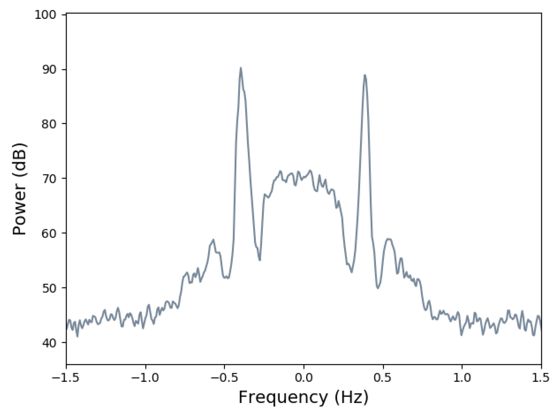
Coastal high frequency or HF radar (3–30 MHz) is a tool that has enabled users to remotely measure ocean currents, winds and waves, in real-time, since the initial observation of Crombie [1] in 1955, who realised the relationship between ocean wave and HF radar Doppler spectra (such as that shown in Figure 1). The measurements are important in a number of coastal engineering topics, including testing of and assimilation in operational wave models, sea vessel navigation, land/beach erosion, designing offshore structures, and in supporting marine activities. Additionally, collecting ocean data over a long period of time can be useful in climate changes studies; the same data can also be used to assess the potential of a coastal region to become a wave/wind farm as shown by Wyatt [2]. With such important applications, the accuracy of the measurements is imperative.
The majority of the existing theory is for monostatic radar, where the transmitter and receiver are co-located. Ocean surface current measurements from such a radar are robust, and hundreds of radars provide real-time current measurements all over the world; see the work of Paduan and Washburn [3] for an introduction to the subject. Methods for measuring wind direction and variability are also reliable, such as the method of Wyatt et al. [4], where the maximum likelihood method is used fit the wind distribution to the available radar data. Ocean wave measurements are also possible, however, they can be less robust as they are more vulnerable to noise (for limitations see Wyatt et al. [5]). Notable methods of Lipa [6,7], Howell and Walsh [8], and Hisaki [9] are all significant in the history of measuring the wave spectrum. Another key method is the Seaview method, presented by Wyatt [10], and Green and Wyatt [11], which will be explained in Section 3.
To obtain the ocean measurements using radar data, many researchers use the radar cross section of the ocean surface, which models what the radar output will be for a given ocean state and radar frequency. For monostatic radars, the most commonly used radar cross section is that of Barrick [12,13], derived in 1972, based on the perturbation method of Rice [14]. The expression is split into its first and second order components; the first order radar cross section, , is due to resonance between the emitted radio waves and ocean waves of a particular length and direction, and the second order radar cross section, , is due to double scattering of the emitted radio waves from two ocean waves and the non linear combination of the same two ocean waves. In full, for radar wavenumber and ocean spectrum ,
where , is known as the Bragg wavenumber and
is known as the Bragg frequency, for ocean depth d and gravity g. The second order term is given by
where and , with respective angular frequencies and , are the two contributing wave vectors, defined by the relationship . The term is known as the coupling coefficient and contains the mathematics of the nonlinear combinations of the waves and, as such, is a function of and . More detail on the monostatic coupling coefficient is given by Lipa and Barrick [15].
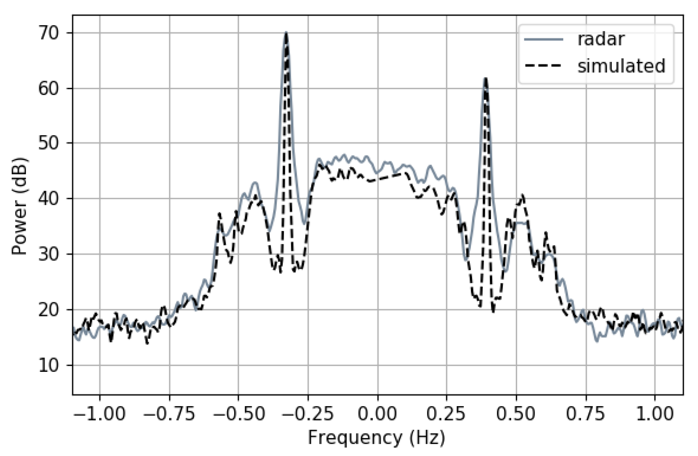
Numerical methods like that of Holden and Wyatt [16] can be used to simulate monostatic Doppler spectra for given ocean conditions and radar settings, using Equations (24) and (28); a comparison of a radar measured Doppler spectrum and a simulated Doppler spectrum, using co-spatial and co-temporal wave buoy data as input to the simulation, is shown in Figure 2 where good agreement is shown.
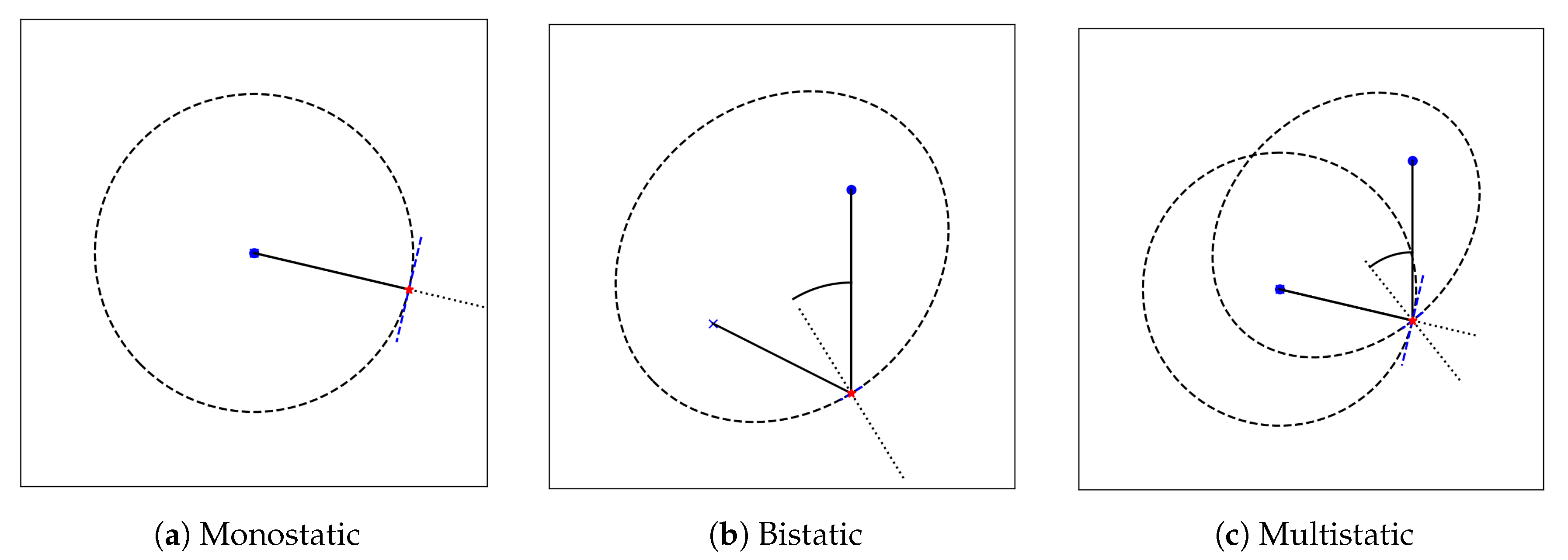
Recently, bistatic radar—where the transmitter and receiver are separated by a notable distance—is on the ascendancy. Therefore, conversely to monostatic radar which receives backscatter, the detected radio waves in a bistatic radar have been scattered at a non-zero angle. A traditional coastal HF radar site consists of two monostatic radars, each providing data from ocean backscatter. However, a third dataset can be obtained at no additional cost if one of the receivers also receives bistatic scatter from the other transmitter. In this case, the radar site is called multistatic. Each different radar setup is shown in Figure 3. The advantages of employing a bistatic/multistatic radar setup are that (1) it can reduce the cost of setting up/maintaining a HF radar and (2) it can increase spatial coverage and data quality as shown by Whelan Hubbard [17].
In this paper, the aim is to obtain directional wave measurements from bistatic radar data. Previously, for bistatic radar, Zhang and Gill [18] developed an inversion algorithm to obtain the nondirectional wave spectrum from bistatic radar data and, when tested on simulated data, they obtained good results. Silva [19] has also presented results of simulated bistatic HF radar data inversion where the directional wave spectrum was estimated using Tikhonov regularization. They achieved good results for simulated data, however, the method is limited as a model is assumed for the direction of the spectrum, and this assumption may not always be appropriate.
In the existing numerical methods for extracting wave measurements from monostatic radar data, the aim is to invert Equation (3), to obtain the ocean spectrum in terms of the measured . Anderson [20] stated that the existing algorithms should work for a bistatic system if the inverted radar cross section is changed to the bistatic expression. In this work, we test this hypothesis and modify the Seaview method to measure the directional wave spectrum from bistatic HF radar data. Therefore, to do this, the bistatic radar cross section must be known.
In 1975, Johnstone [21] presented a bistatic radar cross section of the ocean surface and then, in 2001, Gill and Walsh [22] presented an alternative expression. However, under monostatic conditions, neither of the expressions reduce exactly to the monostatic term of Barrick [12,13] (which the Seaview method depends on). The derivation of Johnstone appears to have an error which causes the difference in the resulting expressions; Gill and Walsh followed a more complicated method, however, it has been shown that the monostatic form of their radar cross section is similar to Barrick’s and it is, therefore, unnecessary to change the existing operational inversion programs to use theirs instead. Another recent derivation is given in Chen et al. [23].
A bistatic radar cross section that reduces exactly to the monostatic term of Barrick [12,13] would be beneficial to systems based on Barrick’s expression (such as the Seaview inversion) as, in the radar coverage area, the bistatic angle can vary between 0° and 90°, so the discontinuity between the monostatic and bistatic radar cross section expressions would cause a discontinuity in the inversion program used and perhaps, then, the results. Therefore, in this work, we follow the method of Barrick, whilst retaining the bistatic angle, to derive the bistatic radar cross section of the ocean surface. A reviewer of this paper has drawn our attention to similar work by Hisaki and Tokuda [24] who allowed for a finite scattering area and showed that their equations reduced to those of Barrick for an infinite scattering area and a monostatic geometry.
We begin with an overview of the derivation of the bistatic radar cross section in Section 2.1, before presenting the numerical solution of the resulting expression in Section 2.2. Details of the Seaview inversion method (for which details of the cross-section equations and numerical simulations are a pre-requisite) are then given in Section 3. The results of the modified Seaview inversion, when tested on simulated bistatic data, are given in Section 4 and these are discussed in Section 5 which also includes some concluding remarks.
2. Materials and Methods
2.1. Bistatic Radar Cross Section of the Ocean Surface
To derive the bistatic radar cross section of the ocean surface, we follow the method of Barrick [12], where the equivalent monostatic radar cross section was derived. In his work, Barrick used the perturbation analysis of Rice [14] where, by assuming small waveheights and slopes, the electric field scattered from the ocean surface, , was calculated. They key points of the derivation follow, however, more details can be found in the work of Hardman [25].
The value of depends on both the incident radio waves and the properties of the scattering surface. Firstly, the incident waves will propagate as vertically polarised ground waves. Secondly, as the ocean varies in both time and space, by assuming that these variations are periodic and that the surface is of infinite extent, we can define the surface, , as a Fourier series expansion, such that
for wavenumber , angular frequency and Fourier coefficients which are dependent on the integers m, n and l.
The electric field scattered from this surface, will also be periodic with the same fundamental spatial and temporal periods and hence Rice defined as a Fourier series. For a perfectly conducting flat surface, the exact solution can be found. Therefore, we perturb the solution around the flat surface, with ordering parameter (for radar wavenumber ), using Maxwell’s equations and the tangential boundary condition to obtain the first and second order Fourier coefficients. Details of the calculations for vertically polarised waves can be found in the work of Hardman [25]; for horizontally polarised waves, the details are provided by Rice [14]. The resulting scattered electric field has components
where is the angular frequency of the emitted radio waves,
in which
and
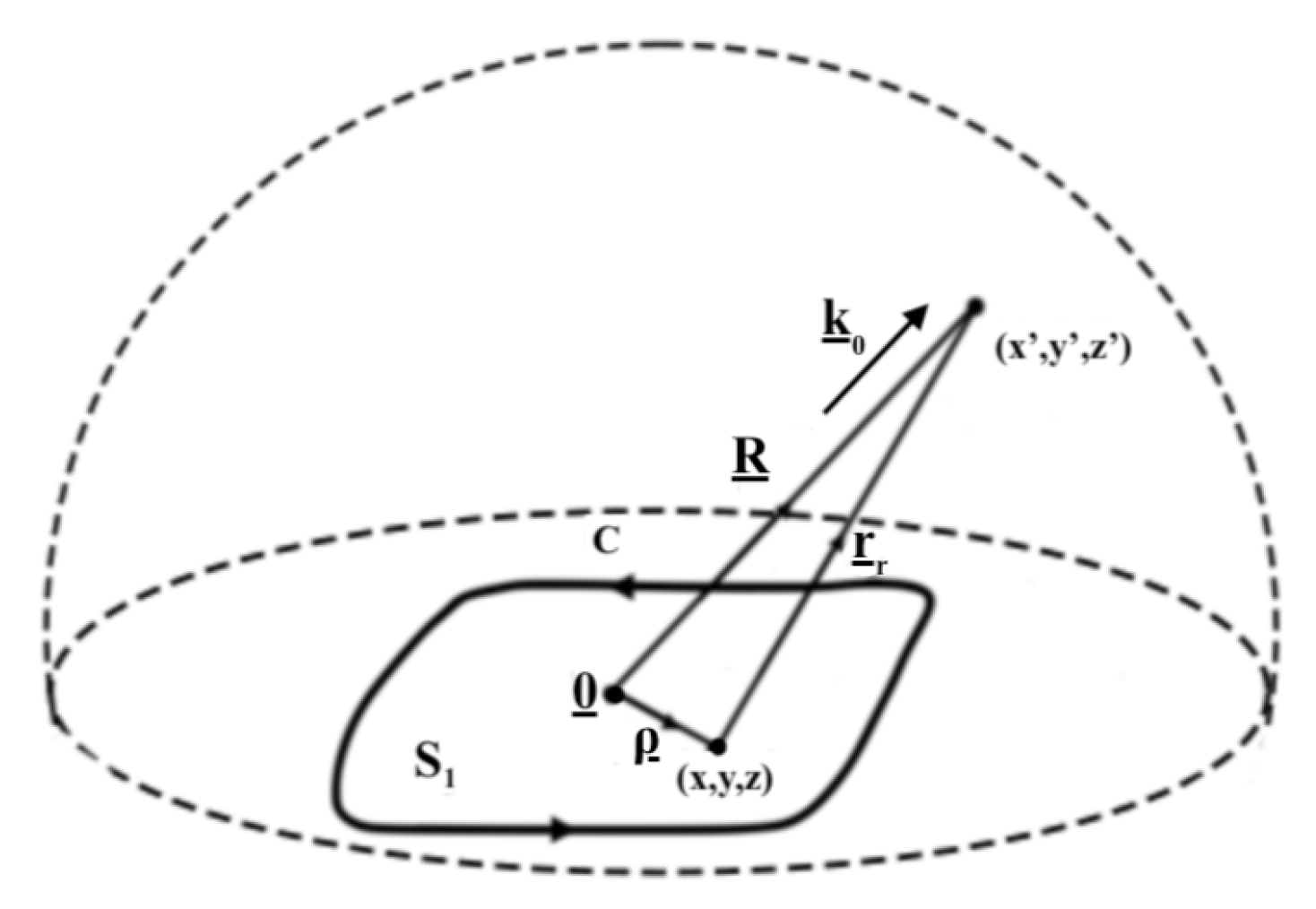
By definition, the electric field in Equations (5)–(7) corresponds to the scattering of infinite plane waves from a surface of infinite extent. To transform the fields to finitely scattered fields, which is necessary as only a portion of the whole ocean will be illuminated by the radar, we can use the equation presented by Johnstone [21] who followed the work of Stratton [26]. He showed that if the electric field is known on a finite section of an infinitely large volume such as the surface on the hemisphere shown in Figure 4, then the scattered electric field at a point inside of the volume can be calculated.
The equation is given by
where is the vector on , are the radius, polar angle and azimuthal angle measured from the origin to and is the radar wavevector given by
Note that the integral can be evaluated on any plane and is used for convenience. However, as pointed out by Hisaki and Tokuda [24], this choice is in fact the infinite scattering surface limit. Evaluating the integral on z = f as they did changes the resulting power spectrum of the scatter but differences are very small at the Doppler frequencies used for inversion so z = 0 is sufficient for this work. To find the scattered field at a point , the values for , and from Equations (5)–(7) are substituted into Equation (8) and the integral is calculated. The vertically polarised component, , is then identified in the resulting expression (as these are the radio waves that the receiver will detect) such that
where,
and,
for and .
In the scattered electric field in Equation (9), the first order components (namely, the terms including a single P term) represent the single scattering of one electromagnetic wave, to the receiver, from one ocean wave. The second order components (which include a factor of Q) represent doubly scattered electromagnetic waves, to the receiver, from two single ocean waves. The order of the ocean wave, currently denoted by , has not yet been considered and is assumed to be first order. However, in making such an assumption, a second order contribution from first order scattering from second order oceans waves is missed, where a second order ocean wave is the result of the nonlinear interaction between two first order ocean waves.
To allow for the second order hydrodynamic effects in shallow water, Barrick and Lipa [27] used a perturbation method to relate the second order coefficients , of a surface defined by , to the first order coefficients . Their method involved expanding the surface height Fourier coefficients around the flat surface, i.e.,
alongside boundary conditions from the equations of motion, also expanded to second order. They showed that for ocean waves with wavevectors and , with corresponding angular frequencies and (related by the dispersion relation of ocean waves given by ),
where , , and
is called the hydrodynamic coupling coefficient.
To include the second order hydrodynamic effects in the scattered electric field, we expand into and then substitute in the value of using Equation (13) (by letting and ), and so Equation (9) becomes
where for brevity
and
Following Johnstone [21], we finally calculate the radar cross section by substituting Equation (15) into
where R is the distance from the scatter patch to the receiver and denotes a Fourier transform, with definition
To calculate Equation (16), the following properties of the surface height Fourier coefficients are used:
- The Fourier coefficients are normally distributed about zero; hence
- As the surface is real, is equal to , which is true when
- The surface roughness spectrum , found by utilising the Wiener–Khinchin theorem, is related to the surface height Fourier coefficients bywhere and .
Then, substituting from Equation (15) into Equation (16) and using Equation (20) leads to
where the arguments of Q are implied. The calculation of Equation (23) can be separated into its first and second order terms, such that
where the first order radar cross section, , is defined by the term including the average , and the second order, , including . To calculate each of and , the properties in Equations (18)–(22) are used to enforce restrictions on the Fourier coefficients and to introduce the roughness spectrum . The mathematical details are spared here, but can be found in the work of Hardman [25].
2.1.1. First Order
2.1.2. Second Order
The second order bistatic radar cross section is
for wavevector pairs and (with respective angular frequencies and ) such that
Explicitly,
and is the electromagnetic coupling coefficient given by
where
is the normalized surface impedance derived by Barrick [29] and
and
(noting that both and can be real or imaginary depending on the argument), where is a unit vector in the direction of the receiver from the scattering patch (see Figure 5), namely,
2.1.3. Monostatic Conditions
When , i.e., under monostatic conditions, the first and second order radar cross section expressions given in Equations (24) and (28), respectively, are equivalent to the commonly used first order monostatic radar cross section of Lipa and Barrick [15], except for a factor of 2. The difference is due to differing Fourier transform definitions, however, the factor is ultimately not important as when the inverse Fourier transform (which will also be different by a factor of 2) is taken to find the power in the spectrum, the two terms will be equal. Furthermore, when inverting the expression, the whole spectrum is normalised to removed the effects of propagation over the ocean and so the factor is again inconsequential.
2.2. Numerical Solution
The method for finding the numerical solution of the bistatic radar cross section given in Equations (24) and (28), is analogous to the method of Holden and Wyatt [16].
2.2.1. First Order
Due to the delta function in Equation (24), the first order contribution to the Doppler spectrum will appear as two peaks at , defined in Equation (25). The contribution comes from two wave vectors, , travelling in the direction of the Bragg bearing, both toward and away from the radar set up. As Crombie [1] hypothesised (for monostatic radar), these particular signals are amplified by resonance. As includes a factor of , for one radar using a single carrier frequency, there will be a number of different Bragg waves, dependent on the radar beam range and angle. Scattering from locations where are referred to as forward scatter and when this occurs, both and tend to 0. Consequently, the wavelengths of the Bragg waves in this region become infinitely long and in addition, the factors in Equations (24) and (28) will tend to zero, leading to a low SNR.
2.2.2. Second Order
The second order radar cross section contribution, given in Equation (28), is due to double electromagnetic scattering from two first order ocean waves, with wavevectors and , and the nonlinear interaction between the same two ocean waves. The wave vector pair sum to give the Bragg wavevector and, theoretically, large numbers of pairs exist in the p, q wavenumber plane; an example pair can be seen in Figure 6. To find the values of and , the solution to the delta function in Equation (28), such that
is sought. For each value of , the set of solutions of and defines a frequency contour in the p, q plane. As m and can both take the values of 1 or , Equation (36) has four different forms.
Case :
Now, as the sum of two sides of a triangle is greater than the third, , and therefore
Taking the square root gives
which is equal to the bragg frequency given in Equation (25). This leads to two conditions;
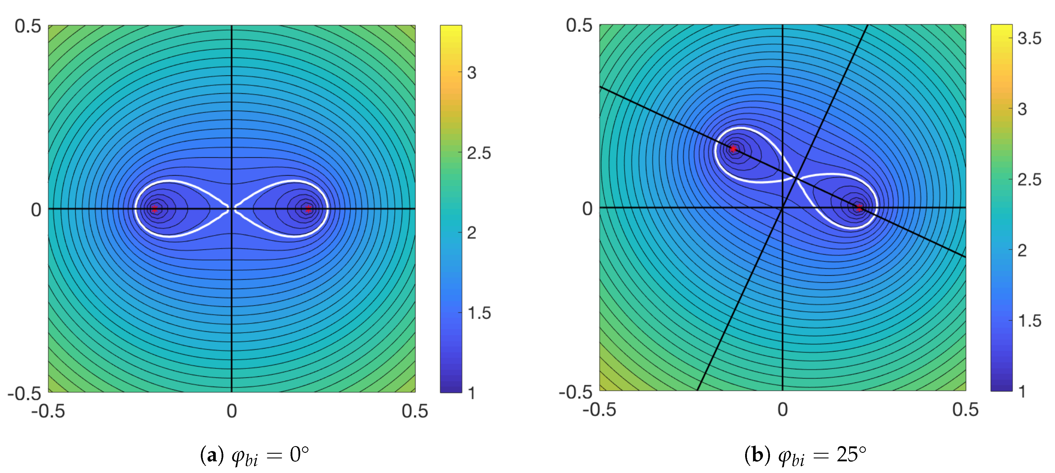
Figure 7 shows the frequency contours, defined by Equation (36). At frequencies close to the Bragg frequencies the contours are circular in shape, centred around the Bragg frequency. As increases, the contours become less circular, until , shown in white in Figure 7, where they separate.
When , the contours are symmetrical about the p and q axes, however, when , the contours rotate clockwise in the p, q plane, becoming symmetrical about some other axes, say and , shown by the additional black lines in Figure 7b.
Case :
In the right hand plane, when and lie in opposite directions along the axis, meeting at a point past the bragg frequency, reaches its maximum value of . Therefore,
and this leads to the conditions
In the left hand plane, where , the result is reversed giving
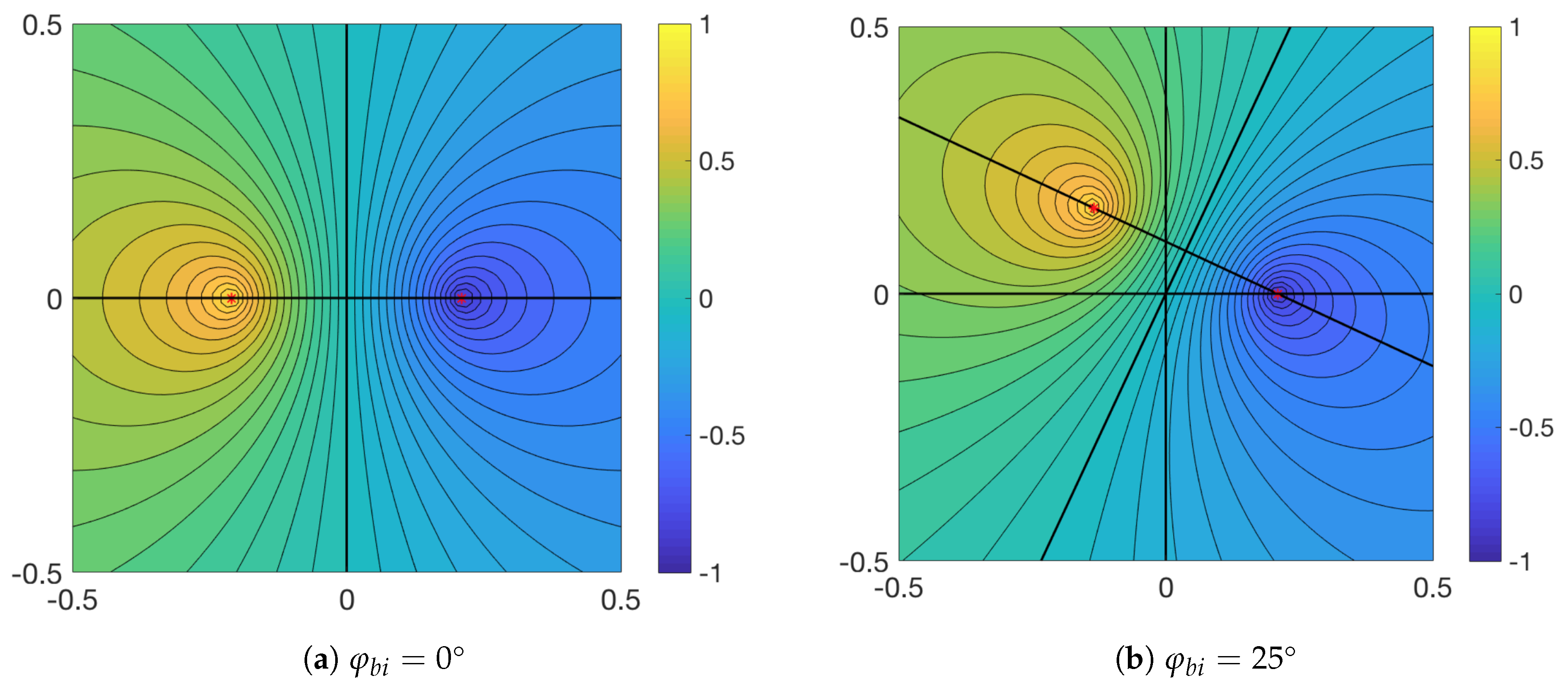
Figure 8 shows the normalised frequency contours when for different values of . Like when , the contours are symmetric about the and axes, however, in this case, they do not cross the axis for any frequency. The contours depict small circles around the Bragg frequencies, growing in size and becoming less circular as the frequency approaches zero.
As the frequency contours for all four possible combinations of m and are symmetrical about the axis, the integration in Equation (28) can be taken over one half of the symmetric plane and doubled. Therefore, we integrate Equation (28) over the right hand plane, and double the result and hence
In the right hand plane, where , we can calculate the integral in polar coordinates and , where is the angle between and the p axis, as shown Figure 6. Explicitly,
where and are the integration limits of and vary with frequency as well as . In general, we find that the integration limits are
however a particular set of values require different limits. This happens when and , as the frequency contours cross the axis and no longer complete full rotations in the right hand plane. By symmetry, when the contours cross the axis, and are the same length. Therefore, when and , the delta constraint of Equation (36) becomes
and then squaring Equation (40) gives
which can be solved numerically for .
Introducing a term, , as the angle between and (see Figure 6), the integration limits are given by
Therefore, as , where the solution for from Equation (41) is used,
In terms of and ,
To calculate , we now reduce the double integral in Equation (38) to a single integral using the delta function. By defining
Equation (38) can be written as
Now, in order to integrate over the delta function, Equation (44) should have an integration variable of h. Therefore, we calculate
where
whose reciprocal is . To integrate over the delta function, the solution, , to
is required, which can be found using a numerical method. For timely convergence in the numerical method, a good initial guess for is important. As the solution for shallow water should not be too different to that for deep water, we find an initial solution for the deep water case and use that, as a starting point, for the shallow water case. The deep water equation can be solved exactly in two cases:
- When and , the solution of is
- When and , the solution is
Upon finding , the second order cross section calculation in Equation (45) reduces to
which can be calculated using a numerical integration method. For speed and convergence we update the value of to the previously found solution for , as incrementally increases.
2.2.3. Electromagnetic Singularities
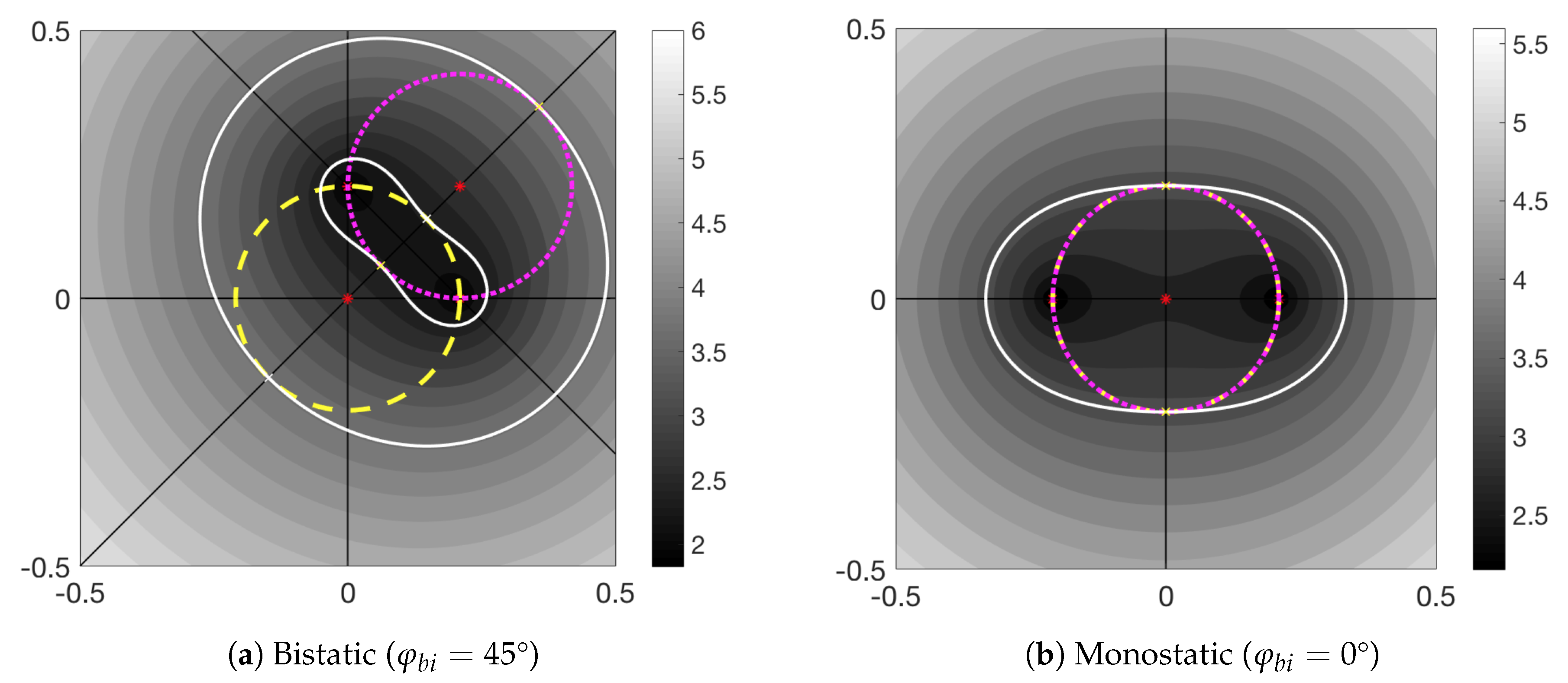
The electromagnetic coupling coefficient given in Equation (30), contains two singularities; either when or is equal to zero. The singularities lie on two circles in the p, q plane, shown in Figure 9; explicitly,
and
Each singularity will be most prominent when a frequency contour is tangential to the singular circle. In order to find the frequencies that this is true for, the solutions for p and q such that the gradient of the frequency contour expression of Equation (36) is equal to the gradient of the circle functions of Equations (50) and (51) are sought. Knowledge of the geometry of the contours and the radii of the circles is exploited to find the solutions for p and q and then the solutions are substituted into Equation (36) to give the tangential frequencies. The four solutions for p and q are
and
Substituting the solutions for p and q, from Equations (52)–(55) into Equation (36) gives two distinct tangential frequencies:
where the solution with the + signs is for the p and q in Equations (52) and (53), and the − signs for the solutions of p and q in Equations (54) and (55).
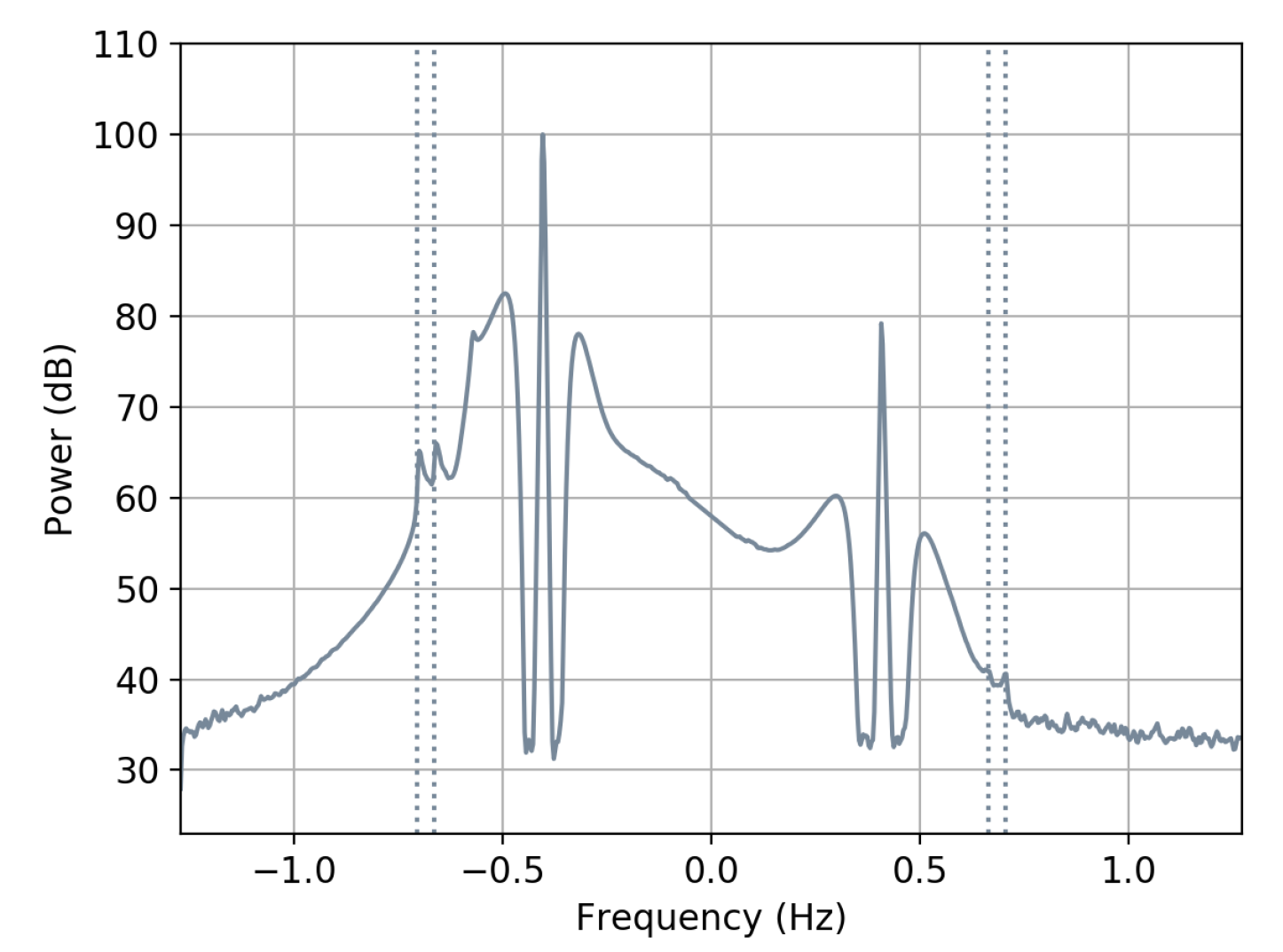
These values for are highlighted in Figure 7 by the white contours and are shown to be tangential to the circles expressed in Equations (50) and (51). Both singularities are highlighted in a simulated Doppler spectrum in Figure 10 by dashed vertical lines. A low amplitude Gaussian noise spectrum has been added as can be seen at the extremities of the plot. For deep water, or when , the values for become
which agree with the results of Gill Walsh [22].
2.2.4. Currents
An ocean current affects how an ocean wave propagates, both in direction and speed. The change in speed means that, because of the Doppler effect, the entire spectrum is subject to an additional shift, . The additional shift is
where is the component of the current velocity in the elliptical normal direction for beam angle .
3. Inversion of to Measure the Directional Wave Spectrum
The aim of inversion is to obtain the ocean wave directional spectrum, , from the power spectrum of the measured radar cross section, using Equations (24) and (28). The power spectrum of the backscattered radar signal is proportional to and therefore in principle needs to be calibrated to account for antenna gains, propagation losses and other factors. To avoid this the problem is usually framed in terms of the ratio of the second and first order backscatter power spectra. A number of inversion methods have been published e.g., [6,8,9,15,16,30]. Here we use the method of Wyatt [10,11] which is referred to in this paper as the Seaview inversion method since Seaview Sensing Ltd has an exclusive license from the University of Sheffield to commercialise the software package and continue its development.
The Seaview Inversion Method
The method used makes the assumption that the first order Bragg wave, , is generated by the local wind and that, by limiting the Doppler frequency range used in the inversion, the waves contributing to the second order scatter can be separated into long waves and short waves the latter also being locally wind-driven. These short wind waves are then modelled with a Pierson–Moskowitz spectrum [31], using an initial waveheight estimate obtained using an empirical method [32], and a sech directional distribution [33] the parameters of which are determined using a wind direction estimation model [4].
The method is iterative and is initialised assuming the wind–wave model applies at all wavenumbers. The ratio of the Equations (1) and (3), , is then integrated to provide a simulated Doppler spectrum ratio which is compared with the measured Doppler spectrum ratio to obtain the difference between them at each Doppler frequency. The wave spectrum is then updated taking into account the calculated Doppler spectrum ratio difference and the value of the coupling coefficient at the long wave vector wavenumber, relative to the maximum along the Doppler frequency contour. The iteration continues until convergence is achieved or a specified number of iterations, usually 100, has been reached. The quality of the convergence is measured by a quantity that reflects the difference between the measured and simulated ratio. The solution can be very different from the initialising spectrum and often shows bimodality in frequency or direction or both due to the presence of swell or changing wind conditions. More details of the method can be found in Wyatt [10], and Green and Wyatt [11]. The maximum frequency (or equivalently wavenumber) of the long waves that can be measured is dependant on the radio frequency [5,34]. The minimum frequency depends on the quality of the radar data which impacts on the ability to clearly separate first and second order parts of the measured Doppler spectrum. An independent validation of the method applied to monostatic data is presented in [35].
The inversion software, providing surface current, wind direction and wave information, was written for monostatic radar configurations only. This has been extended to bistatic configurations using the analysis in Section 2.1 and Section 2.2 above with some modifications to account for a difference in the coordinate system used in the Seaview software. The bistatic extension is not yet part of the commercial package. It has been tested using simulated data, using the methods given in Section 2.2, of two types: (a) two monostatic radars (in order to check that the bistatic extension to the Seaview package provides the same results for zero bistatic angle as the original monostatic package); (b) one monostatic and one bistatic radar sharing a transmitter at the monostatic site. Tests using two bistatic radars with a transmitter between the two sites are in progress but the results are not ready to be reported on at this time. The two receiver sites are those of the University of Plymouth wavehub WERA radar [36,37] and a limited number of cells from the coverage grid for that radar have been used to provide different bistatic angles for the simulations. Using an existing configuration made it easier to provide data for the inversions in standard Seaview formats. The wave parameters used in each simulation are the same at all cells and propagations losses and any antenna effects are not included so the only differences at each cell are the bistatic angle and the Bragg wave bearing relative to wave, wind and current directions.
The wave parameters for the different simulations are described in Table 1. They include modelled and buoy-measured wave spectra.
4. Results
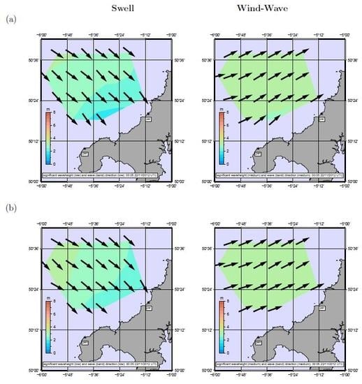
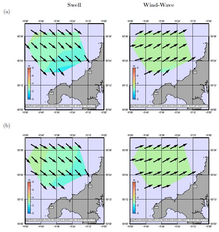
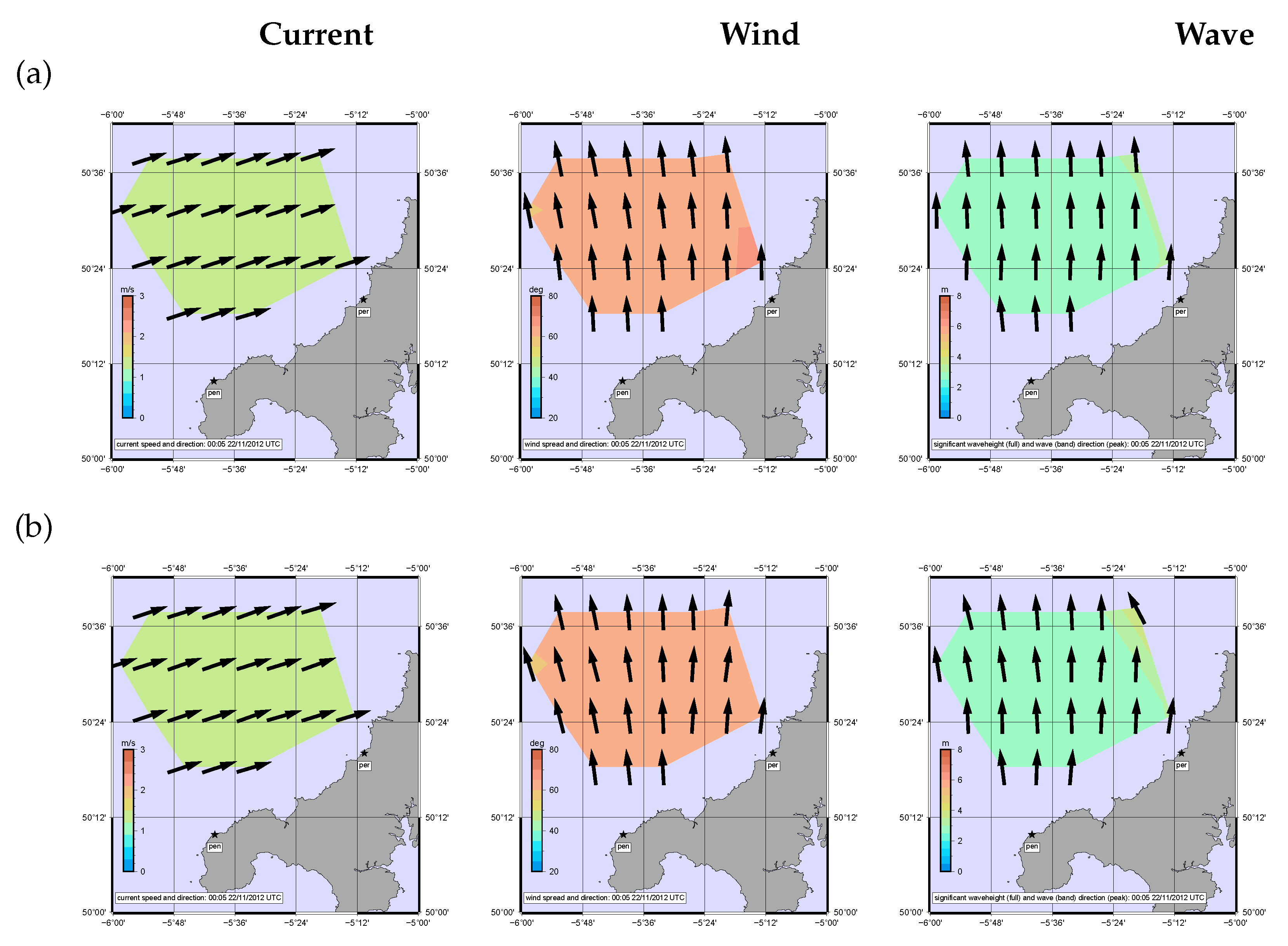
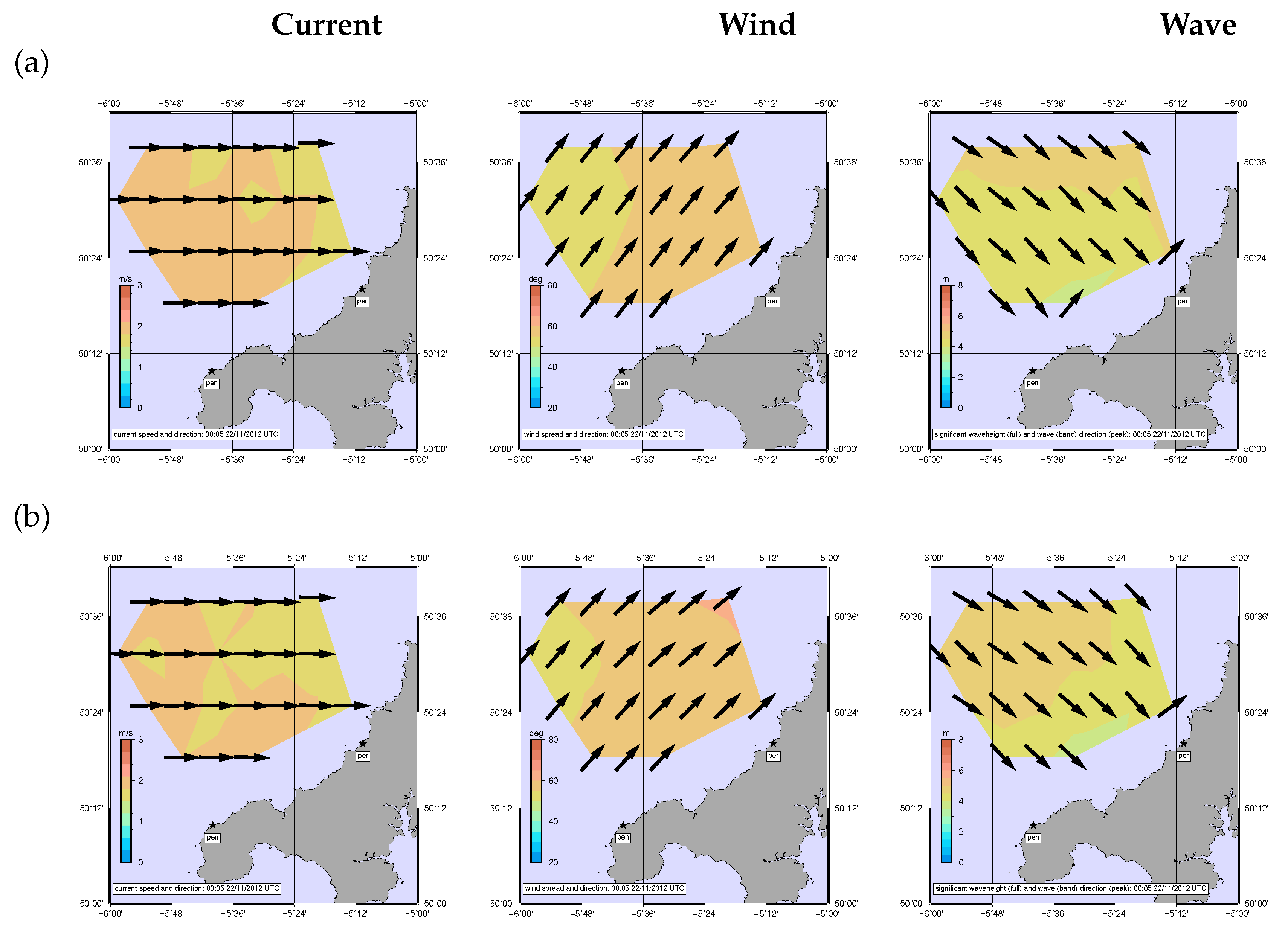
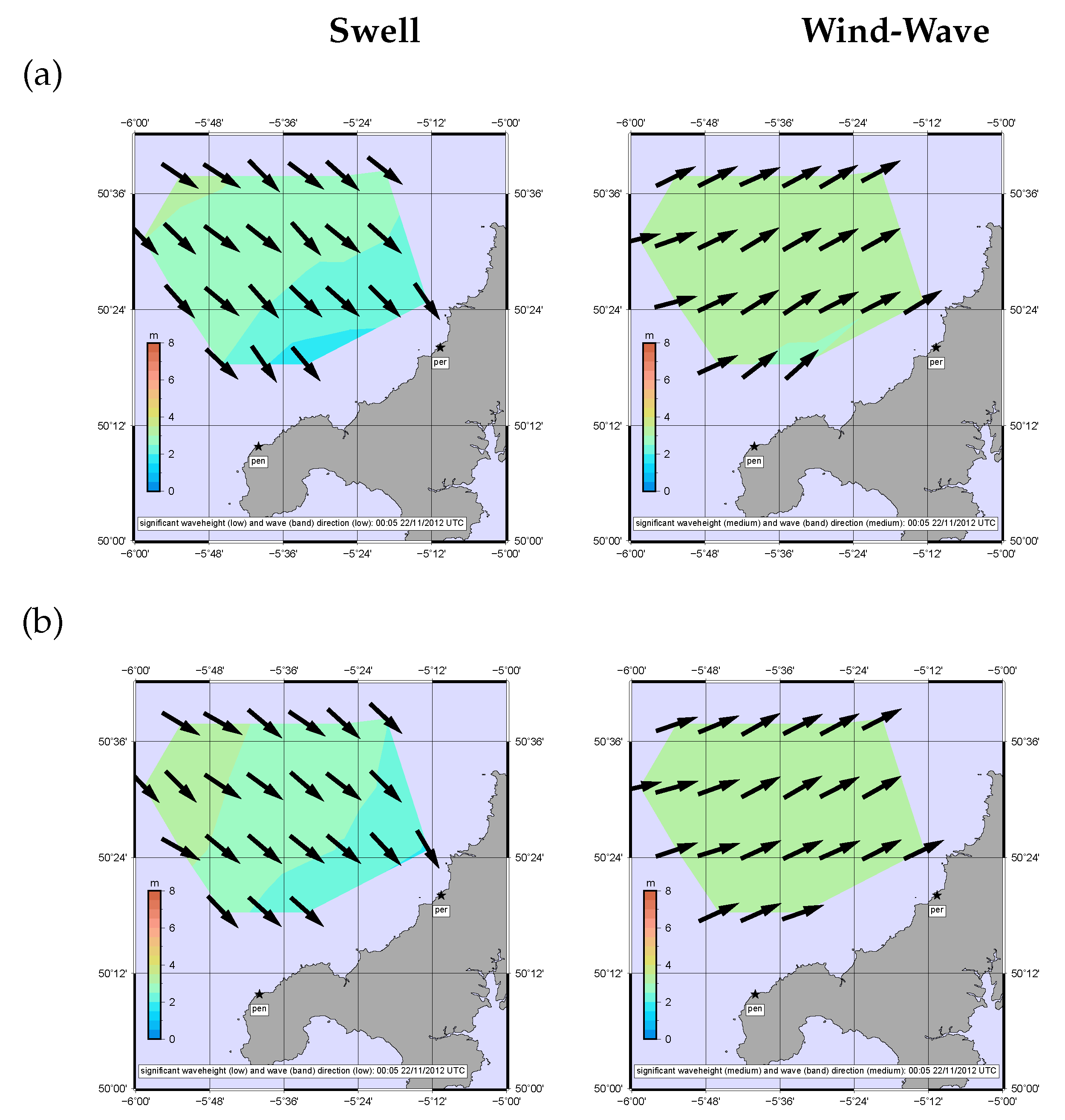
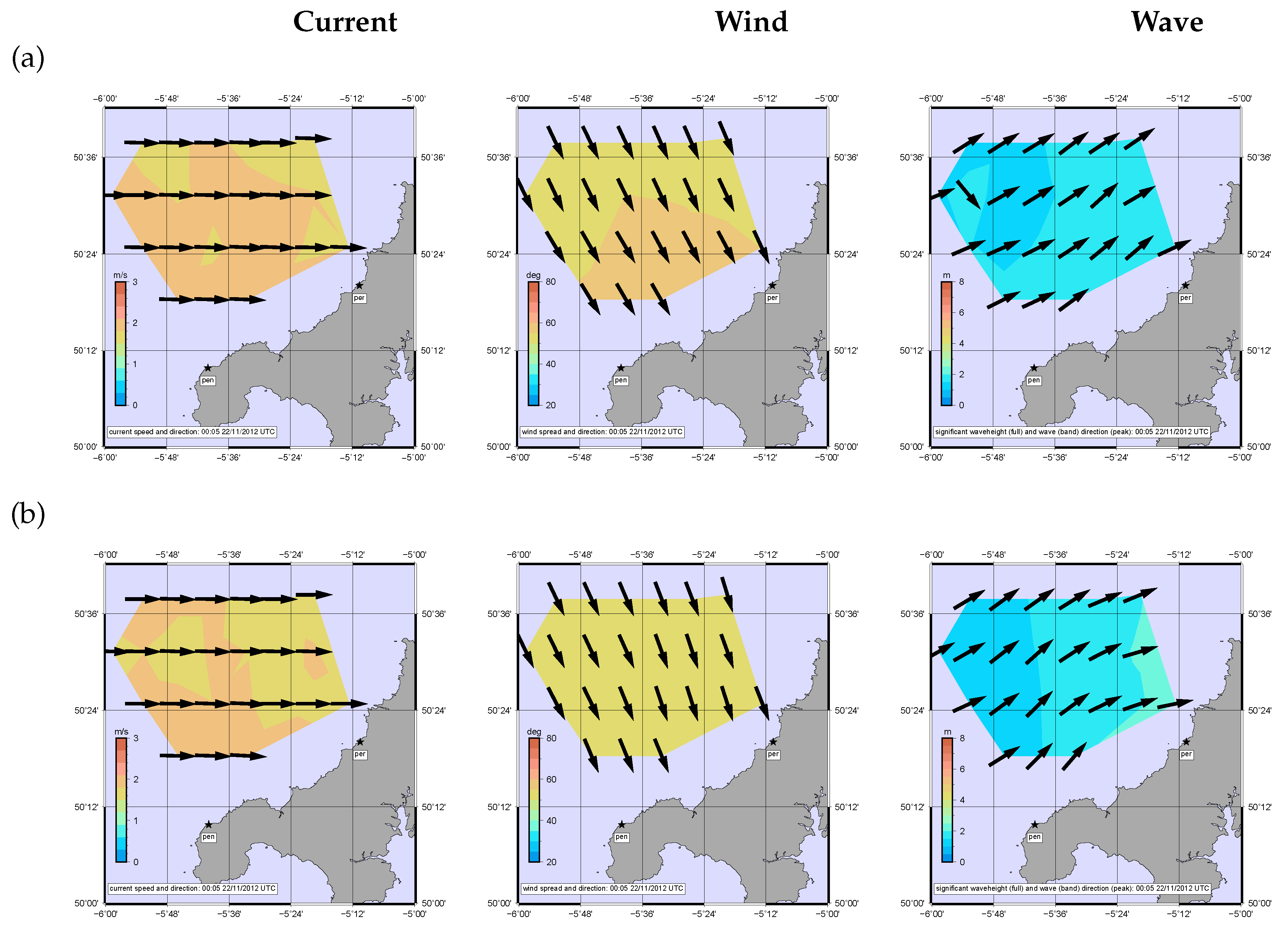
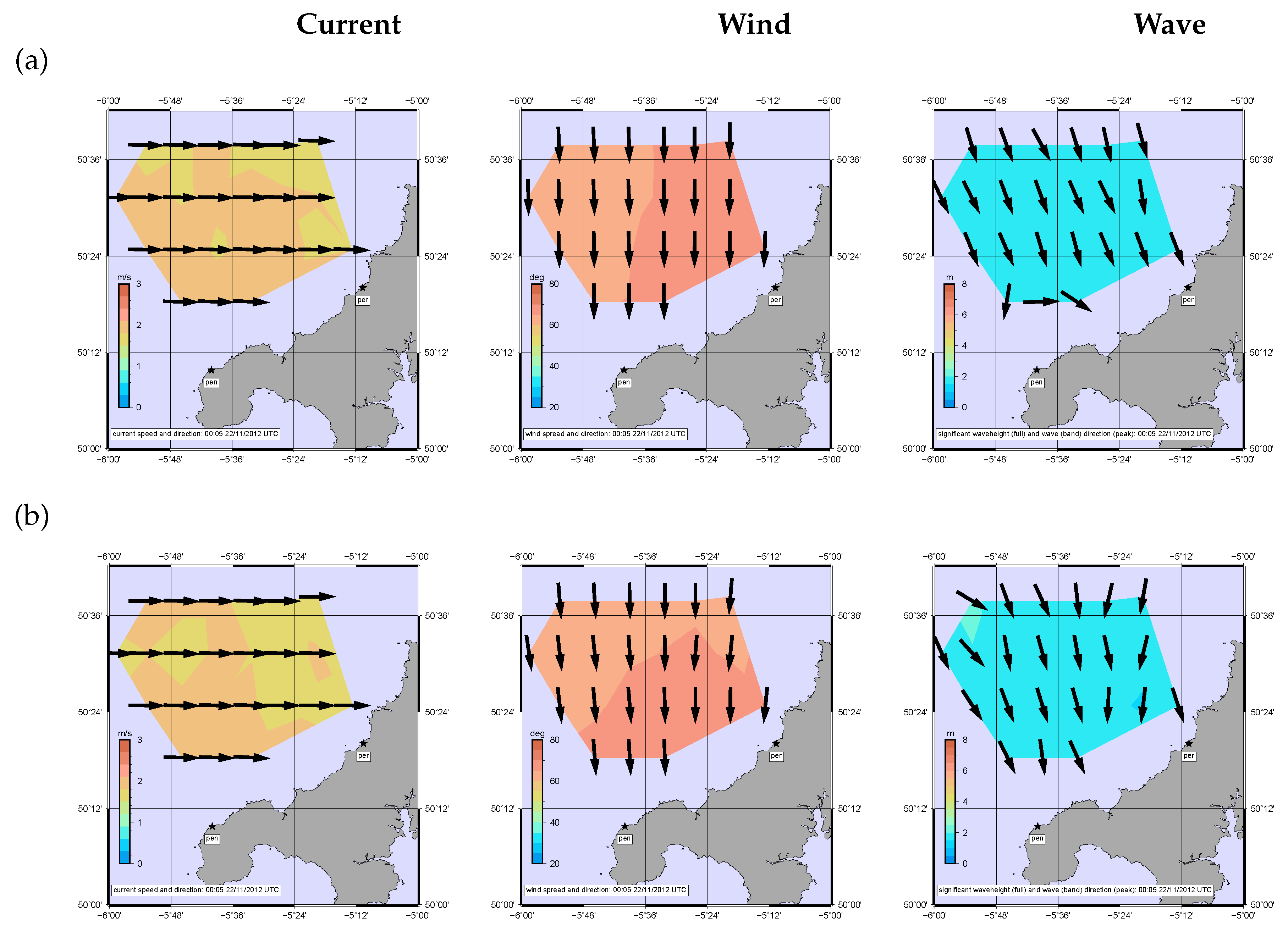
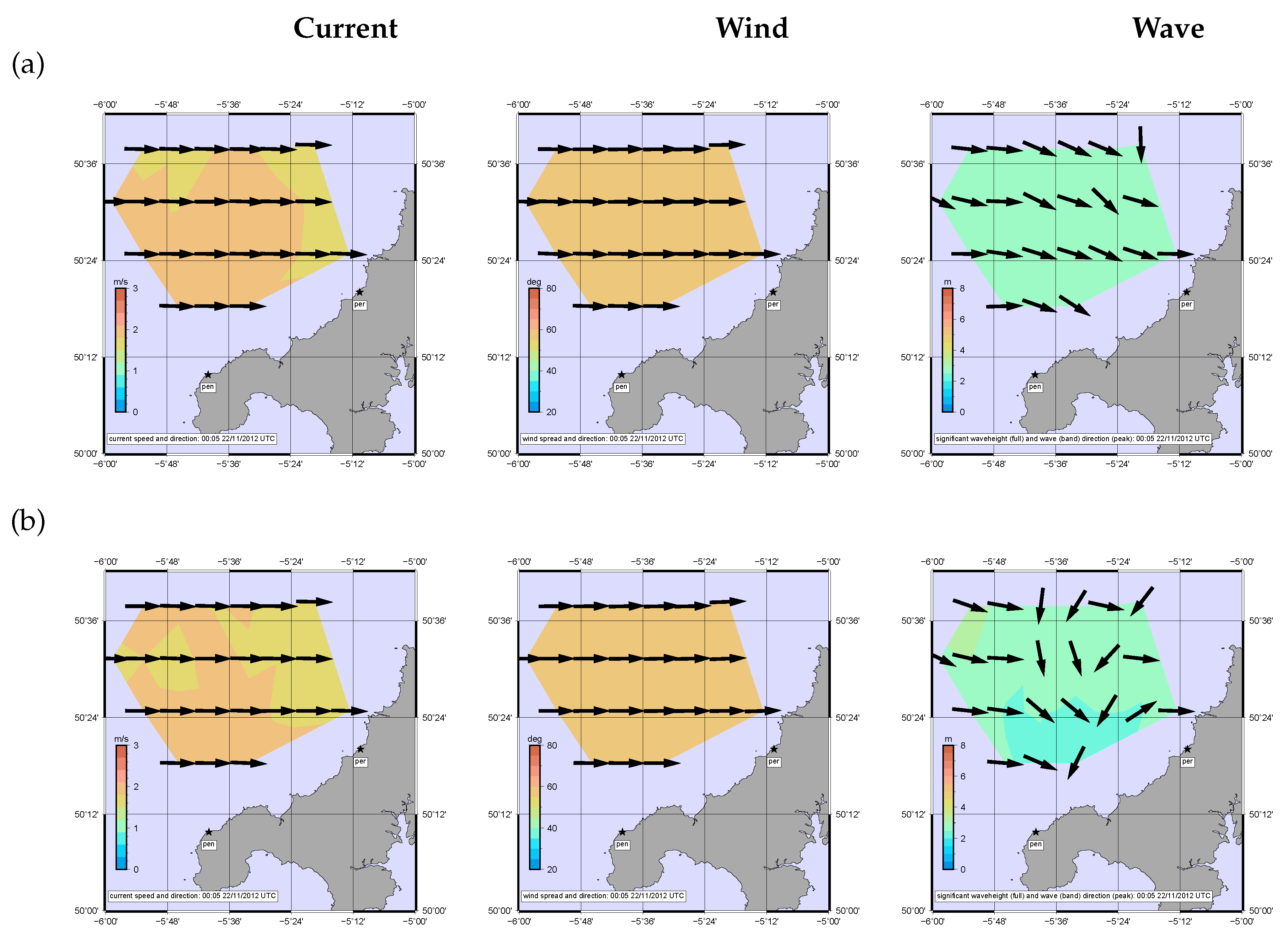
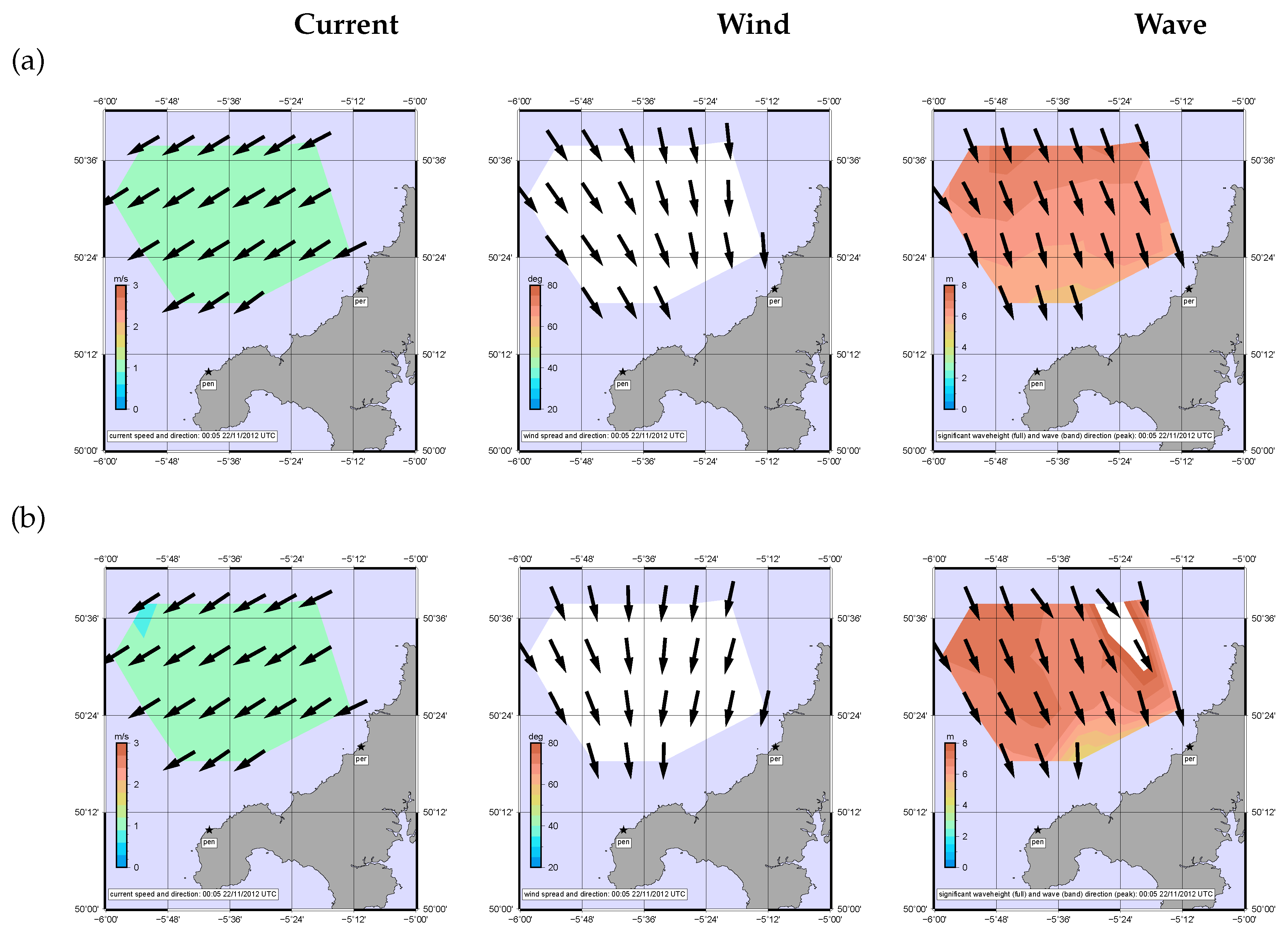
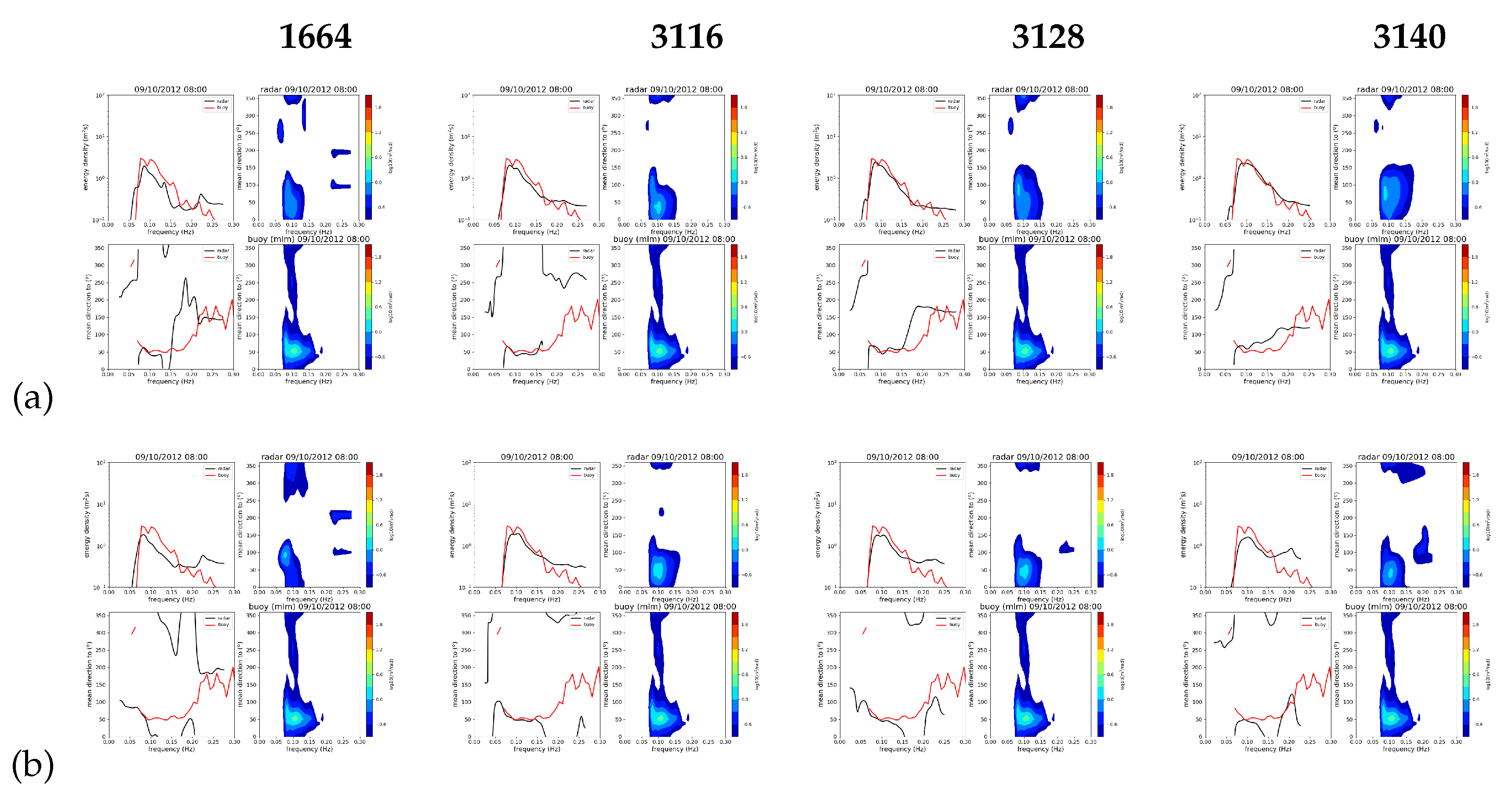
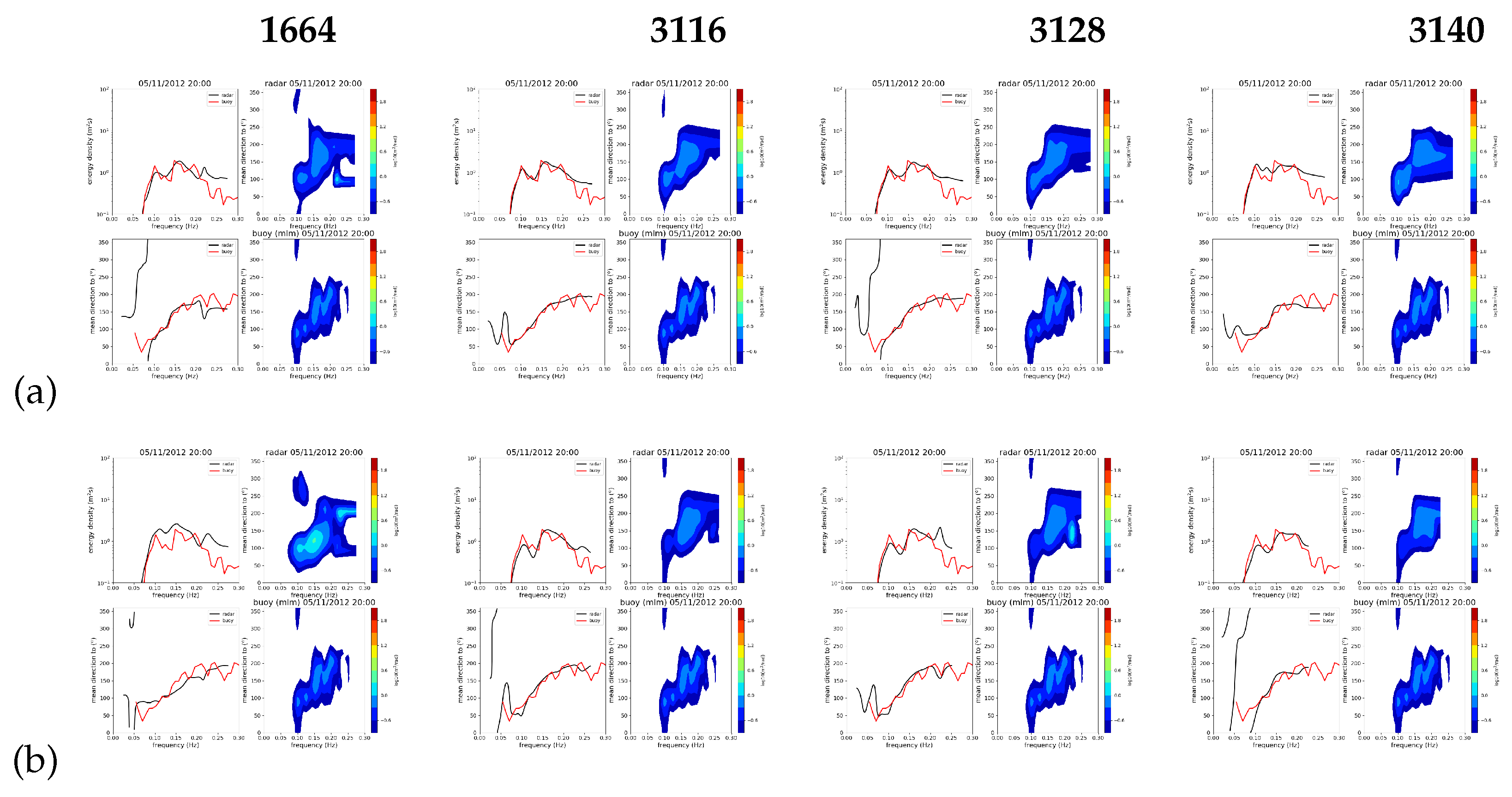
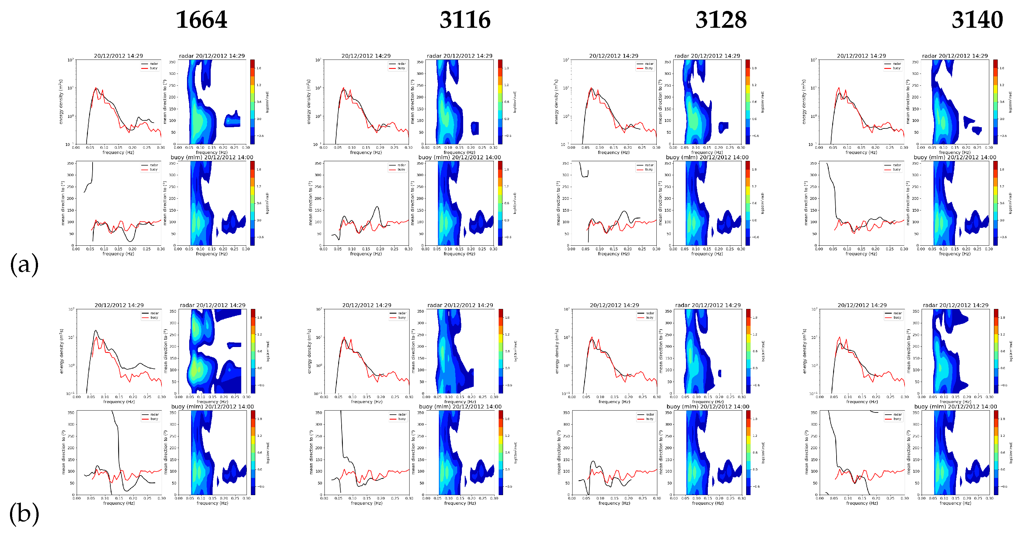
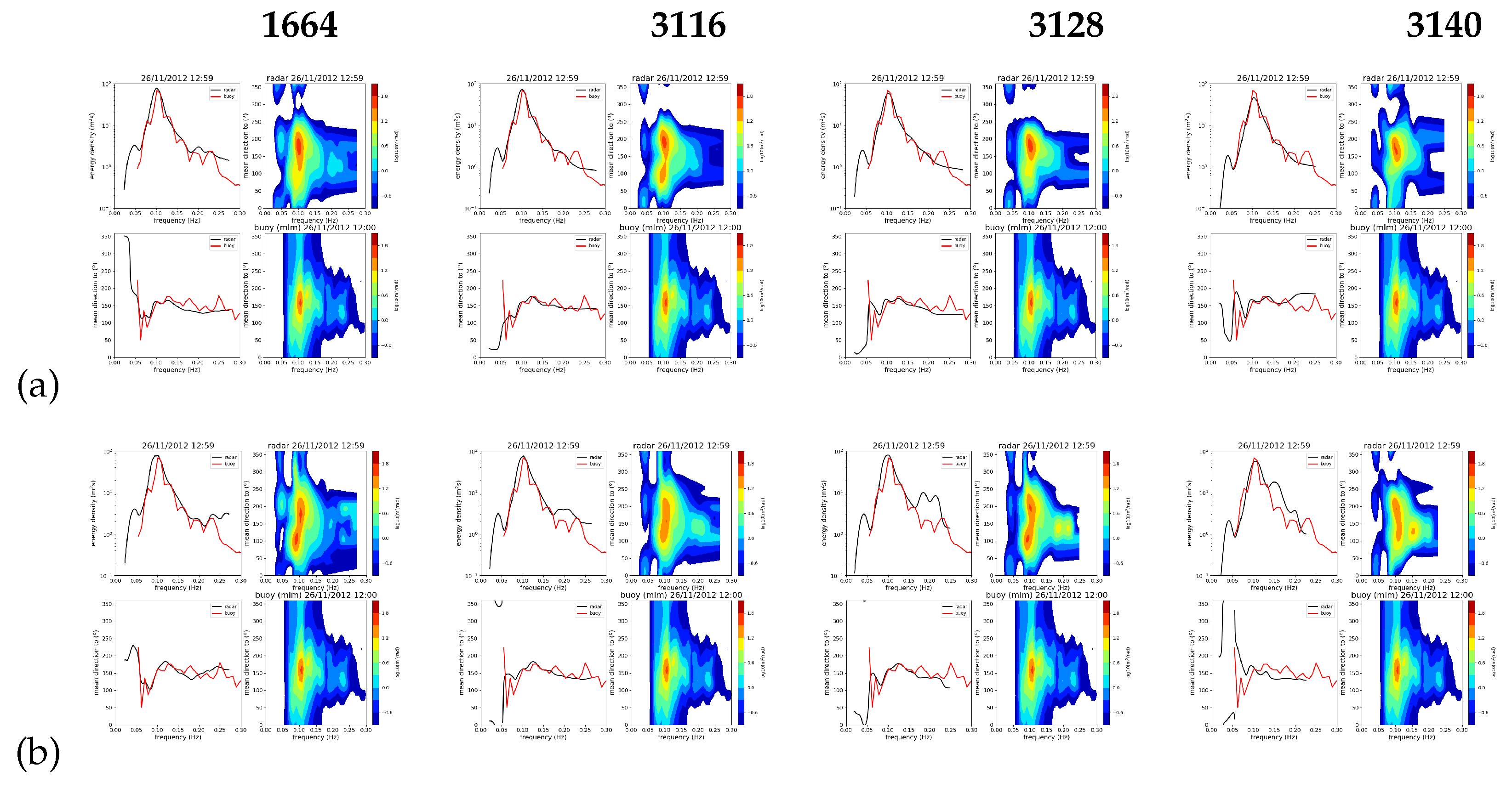
Figure 11 and Figure 12 show inverted surface current speed and direction, wind direction and significant waveheight and spectral peak direction maps for the model cases in Table 1 for the monostatic and bistatic configurations. For the bimodal case 2, Figure 13 shows the long (swell, here defined as waves in 0.05-0.1Hz band) and short (wind–wave, 0.1–0.2Hz) contributions separately to confirm that the latter are aligned with the wind. Figure 14, Figure 15, Figure 16 and Figure 17 show current, wind and wave maps for the buoy cases. Figure 18, Figure 19, Figure 20 and Figure 21 show sample directional spectra compared with those measured by the buoy and used in the simulations to provide a qualitative validation of the radar measured spectra. They are from 4 selected locations to cover the key parameter ranges expected to be important in the accuracy of the inversion. The key parameters are the bistatic angles and the difference in angle between the two Bragg directions (a minimum of is required for monostatic processing [38]) and are presented in Table 2. Note that for some of the locations the Bragg angle difference is below the suggested monostatic threshold. Cell 1664 is the one on the left of the top row in the maps, cells 3116, 3128 and 3140 are the lower three going south along the column to the east of .
There is generally good agreement both for both the standard monostatic and the bistatic case. Differences will be discussed further in the next section.
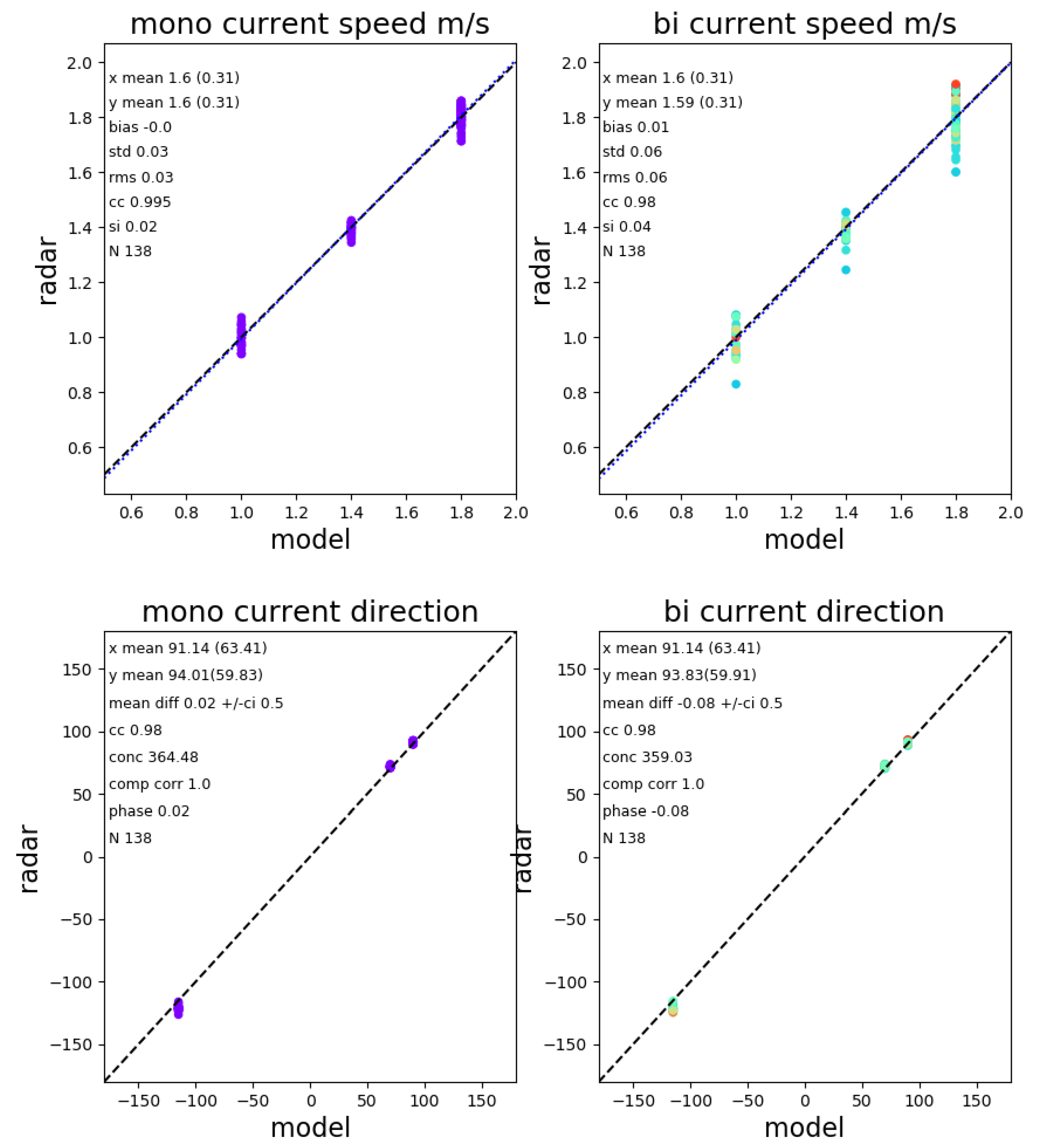
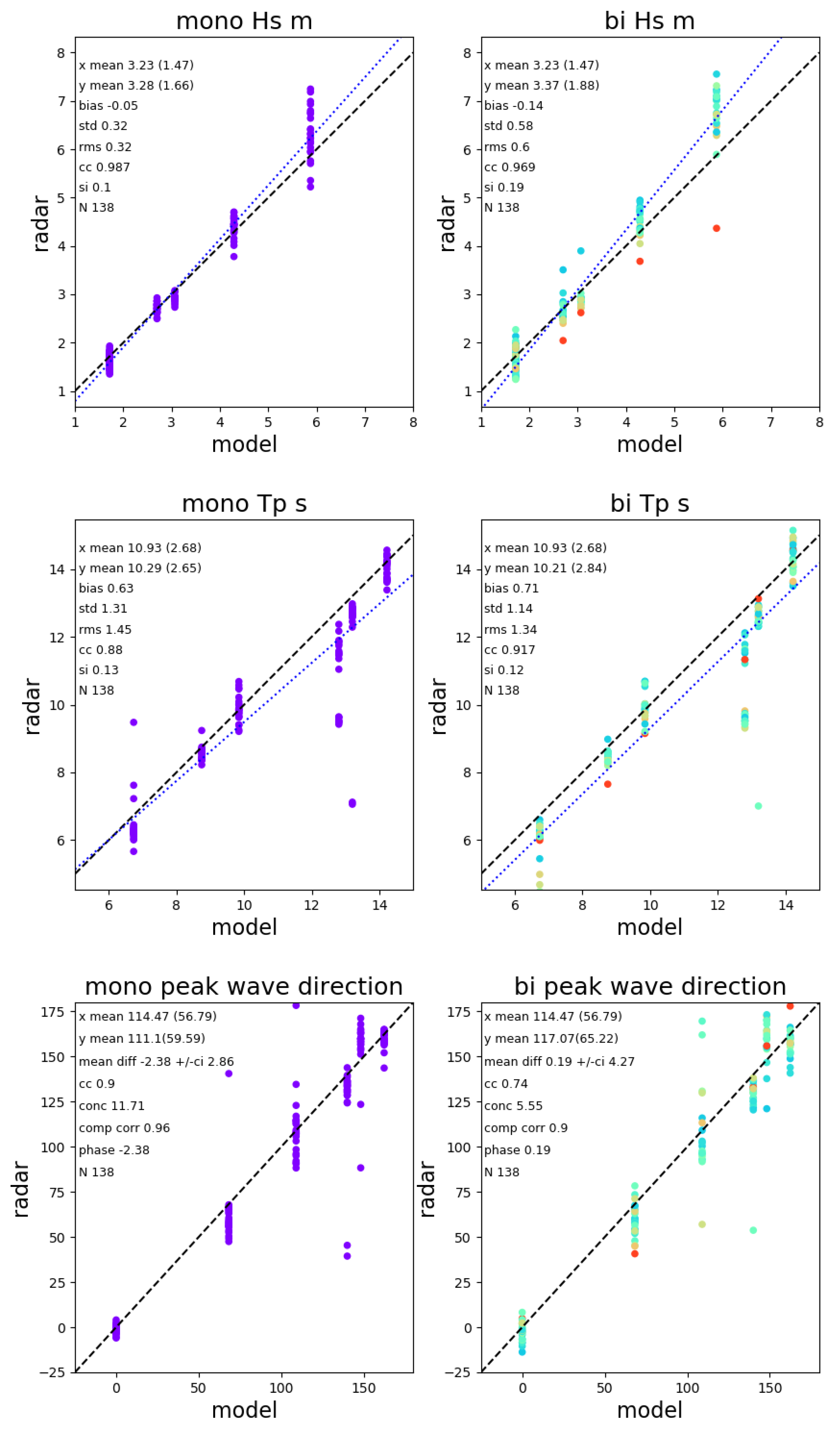
Scatter plots and statistics of the comparisons for currents are presented in Figure 22 and for waves in Figure 23. The data are colour-coded according to the bistatic angle with red being the largest bistatic angle. There is some dependence of the accuracy of the wave measurements on this parameter as can be seen in the right hand column of Figure 23. Most of the larger differences in peak period and peak direction are associated with the bimodal model case where the swell and wind–waves peaks were of similar magnitude and small differences in these magnitudes can lead to differences in peak identification. This is also evident when comparing Figure 12 with Figure 13.
5. Discussion
Monostatic and bistatic radar data have been simulated using the backscatter cross-section formulations developed in Section 2. The Seaview software package has been modified to include bistatic configurations and inverted to provide current, wind direction and wave measurements.
Currents have been obtained with good accuracy and consistency over many different bistatic and Bragg angles as evidenced in the scatter plots, Figure 22, and maps.
Wind directions are consistent with modelling except for the case shown in Figure 17. Note that the colour-coding in the wind plots is the derived directional spreading of the short waves which we haven’t attempted to validate at this point. In Figure 17 this goes beyond the expected maximum () for this parameter. The reason is that the simulation used a wind direction that was roughly aligned with the Bragg direction and the smaller Bragg peak was mostly lost in the simulated noise level. The Seaview algorithm has difficulty estimating a wind direction accurately in these circumstances which, in our experience, rarely occur in measured data. It is interesting to note that waves are still measurable in these conditions confirming that the inversion result is independent of the initial guess which uses the wind direction.
The wave inversions are not as uniform as those for currents and winds. The significant waveheights are in reasonable agreement, Figure 23, although there is some evidence of overestimation at the highest simulated waveheight. That figure also shows that waveheight is underestimated for the largest bistatic angles of . More work is needed to determine a bistatic angle threshold for accurate wave measurement. Case 5 shows particularly noisy peak wave directions, Figure 16, including at the selected cells for which directional spectra are shown in Figure 20. While the frequency spectra (top left in each case) show good agreement, the low frequency part of the mean directions as a function of frequency (bottom left in each case) are not good at the low frequency peaks for three of these cases particuarly for the bistatic case. The inversion seems to be oversensitive to noise at these frequencies, which correspond with Doppler frequencies near the first order peak, and this needs further work as has been noted in many other applications of this method ([34,39]). Although some locations, including cell 1664, have Bragg angle differences in the bistatic case that are below the suggested monostatic angle threshold, there is no evidence that the results are worse there. This aspect also needs further work.
The directional spectra in Figure 18, Figure 19, Figure 20 and Figure 21 use log scales for both the frequency spectra (top left) and the directional spectra (right column) so that differences at both high and low amplitudes can be identified. Apart from the low frequency issue referred to above, the shape of the spectra are in good agreement in all cases. As mentioned above, the maximum frequency for the radar measurements is variable and depends on geometrical factors such as Bragg direction relative to wind direction. At the frequency (12.355 MHz) of the examples presented her, the monostatic cases have maximum frequencies in the range of 0.22–0.283 Hz and the bistatic in the range of 0.187–0.277 Hz.
6. Conclusions
In this paper, the theory for the interpretation of bistatic radar Doppler spectra in terms of currents, winds and waves has been reviewed and methods to simulate and then invert such data have been developed. As far as the authors are aware this is the first time that ocean wave directional spectra, to a maximum frequency that depends on the geometrical parameters and without any prior assumptions about the shape of those spectra, have been obtained from bistatic, albeit only simulated, data. The next step will be to apply the method to measured radar data.
Current, wind and wave measurements from bistatic radar data have been obtained with reasonable accuracy. The statistics for the bistatic cases are not quite as good as the monostatic cases, although they are biased by the large bistatic angle cases. The exact limits on bistatic angle and angle between Braggs still need to be determined but are expected to be about and respectively.
The results in this paper compare a monostatic configuration with a combined monostatic and bistatic configuration with one transmitter at one of the receive sites. Work on a configuration involving two bistatic radars with one transmitter located between the two sites is in progress. This will help to determine suitable configurations for bistatic radar installations for oceanographic measurements.
Author Contributions
Conceptualization, R.L.H., L.R.W.; methodology, R.L.H., L.R.W.; software, C.C.E., L.R.W., R.L.H.; validation, R.L.H., L.R.W.; formal analysis, R.L.H., L.R.W.; investigation, R.L.H., L.R.W.; resources, R.L.H., L.R.W.; data curation, R.L.H., L.R.W.; writing–original draft preparation, R.L.H., L.R.W.; writing–review and editing, L.R.W.; visualization, R.L.H., L.R.W.; supervision, L.R.W.; project administration, L.R.W.; funding acquisition, R.L.H., L.R.W. All authors have read and agreed to the published version of the manuscript.
Funding
This research was partly funded by the UK Engineering and Physical Sciences Research Council (grant number: X/008627-14). The contributions of L.R.W. and C.C.E. were funded by The University of Sheffield and the APC by the UKRI block grant administered by UoS.
Conflicts of Interest
R.L.H. and C.C.E. declare no conflict of interest. L.R.W. is the Technical Director of Seaview Sensing Ltd but her role in this paper is as a University of Sheffield Professor and, as such, makes only scientific inputs and judgements on the work. The funders had no role in the design of the study; in the collection, analyses, or interpretation of data; in the writing of the manuscript, or in the decision to publish the results.
References
- Crombie, D.D. Doppler spectrum of sea echo at 13.56 Mc./s. Nature 1955, 175, 681–682. [Google Scholar] [CrossRef]
- Wyatt, L.R. Wave and Tidal Power measurement using HF radar. In Proceedings of the Oceans 2007-Europe, Aberdeen, UK, 18–21 June 2007; pp. 1–5. [Google Scholar]
- Paduan, J.D.; Washburn, L. High-frequency radar observations of ocean surface currents. Annu. Rev. Mar. Sci. 2013, 5, 115–136. [Google Scholar] [CrossRef] [PubMed] [Green Version]
- Wyatt, L.R.; Ledgard, L.; Anderson, C. Maximum-likelihood estimation of the directional distribution of 0.53-Hz ocean waves. J. Atmos. Ocean. Technol. 1997, 14, 591–603. [Google Scholar] [CrossRef]
- Wyatt, L.R. Limits to the inversion of HF radar backscatter for ocean wave measurement. J. Atmos. Ocean. Technol. 2000, 17, 1651–1666. [Google Scholar] [CrossRef]
- Lipa, B.J. Derivation of directional ocean-wave spectra by integral inversion of second-order radar echoes. Radio Sci. 1977, 12, 425–434. [Google Scholar] [CrossRef]
- Lipa, B.J. Inversion of second-order radar echoes from the sea. J. Geophys. Res. Ocean. 1978, 83, 959–962. [Google Scholar] [CrossRef]
- Howell, R.; Walsh, J. Measurement of ocean wave spectra using narrow-beam HE radar. IEEE J. Ocean. Eng. 1993, 18, 296–305. [Google Scholar] [CrossRef]
- Hisaki, Y. Nonlinear inversion of the integral equation to estimate ocean wave spectra from HF radar. Radio Sci. 1996, 31, 25–39. [Google Scholar] [CrossRef]
- Wyatt, L.R. A relaxation method for integral inversion applied to HF radar measurement of the ocean wave directional spectrum. Int. J. Remote Sens. 1990, 11, 1481–1494. [Google Scholar] [CrossRef]
- Green, J.J.; Wyatt, L.R. Row-action inversion of the Barrick–Weber equations. J. Atmos. Ocean. Technol. 2006, 23, 501–510. [Google Scholar] [CrossRef]
- Barrick, D.E. First-order theory and analysis of MF/HF/VHF scatter from the sea. IEEE Trans. Antennas Propag. 1972, 20, 2–10. [Google Scholar] [CrossRef] [Green Version]
- Barrick, D.E. Remote Sensing of Sea State by Radar. In Remote Sensing of the Troposphere; Derr, V.E., Ed.; GPO: Washington, DC, USA, 1972; Chapter 12. [Google Scholar]
- Rice, S.O. Reflection of electromagnetic waves from slightly rough surfaces. Commun. Pure Appl. Math. 1951, 4, 351–378. [Google Scholar] [CrossRef]
- Lipa, B.J.; Barrick, D.E. Extraction of sea state from HF radar sea echo: Mathematical theory and modeling. Radio Sci. 1986, 21, 81–100. [Google Scholar] [CrossRef]
- Holden, G.J.; Wyatt, L.R. Extraction of sea state in shallow water using HF radar. In IEE Proceedings F (Radar and Signal Processing); IET: London, UK, 1992; Volume 139, pp. 175–181. [Google Scholar]
- Whelan, C.; Hubbard, M. Benefits of multi-static on HF Radar networks. In Proceedings of the OCEANS’15 MTS/IEEE Washington, Washington, DC, USA, 19–22 October 2015; pp. 1–5. [Google Scholar]
- Zhang, J.; Gill, E.W. Extraction of ocean wave spectra from simulated noisy bistatic high-frequency radar data. IEEE J. Ocean. Eng. 2006, 31, 779–796. [Google Scholar] [CrossRef]
- Silva, M.T. A Nonlinear Approach to Ocean Wave Spectrum Extraction From Bistatic HF-Radar Data. Master’s Thesis, Faculty of Engineering and Applied Science, Memorial University of Newfoundland, St. John’s, NL, Canada, 2017. [Google Scholar]
- Anderson, S. Directional wave spectrum measurement with multistatic HF surface wave radar. In Proceedings of the IEEE 2000 International Geoscience and Remote Sensing Symposium, Honolulu, HI, USA, 24–28 July 2000; Volume 7, pp. 2946–2948. [Google Scholar]
- Johnstone, D.L. Second-Order Electromagnetic and Hydrodynamic Effects in High-Frequency Radio-Wave Scattering from the Sea; Technical Report, DTIC Document; Stanford University: Stanford, CA, USA, 1975. [Google Scholar]
- Gill, E.; Walsh, J. High-frequency bistatic cross sections of the ocean surface. Radio Sci. 2001, 36, 1459–1475. [Google Scholar] [CrossRef]
- Chen, Z.; Li, J.; Zhao, C.; Ding, F.; Chen, X. The Scattering Coefficient for Shore-to-Air Bistatic High Frequency (HF) Radar Configurations as Applied to Ocean Observations. Remote Sens. 2019, 11, 2978. [Google Scholar] [CrossRef] [Green Version]
- Hisaki, Y.; Tokuda, M. VHF and HF sea echo Doppler spectrum for a finite illuminated area. Radio Sci. 2001, 36, 425–440. [Google Scholar]
- Hardman, R.L. Remote Sensing of Ocean Winds and Waves With Bistatic HF Radar. Ph.D. Thesis, School of Mathematics and Statistics, University of Sheffield, Sheffield, UK, 2019. [Google Scholar]
- Stratton, J.A. Electromagnetic Theory; John Wiley Sons: Hoboken, NJ, USA, 2007. [Google Scholar]
- Barrick, D.E.; Lipa, B.J. The second-order shallow-water hydrodynamic coupling coefficient in interpretation of HF radar sea echo. IEEE J. Ocean. Eng. 1986, 11, 310–315. [Google Scholar] [CrossRef]
- Thomas, J.B. An Introduction to Statistical Communication Theory; Wiley: Hoboken, NJ, USA, 1969. [Google Scholar]
- Barrick, D.E. Theory of HF and VHF propagation across the rough sea, 1, The effective surface impedance for a slightly rough highly conducting medium at grazing incidence. Radio Sci. 1971, 6, 517–526. [Google Scholar] [CrossRef]
- Hashimoto, N.; Tokuda, M. A Bayesian approach for estimating directional spectra with HF radar. Coast. Eng. J. 1999, 41, 137–149. [Google Scholar] [CrossRef]
- Pierson, W.J.; Moskowitz, L. A proposed spectral form for fully developed wind seas based on the similarity theory of SA Kitaigorodskii. J. Geophys. Res. 1964, 69, 5181–5190. [Google Scholar] [CrossRef]
- Wyatt, L.R. An evaluation of wave parameters measured using a single HF radar system. Can. J. Remote Sens. 2002, 28, 205–218. [Google Scholar] [CrossRef]
- Donelan, M.A.; Hamilton, J.; Hui, W. Directional spectra of wind-generated ocean waves. Phil. Trans. R. Soc. Lond. A 1985, 315, 509–562. [Google Scholar] [CrossRef]
- Wyatt, L.R.; Green, J.J.; Middleditch, A. HF radar data quality requirements for wave measurement. Coast. Eng. 2011, 58, 327–336. [Google Scholar] [CrossRef]
- Lopez, G.; Conley, D.C. Comparison of HF Radar Fields of Directional Wave Spectra against in Situ Measurements at Multiple Locations. J. Mar. Sci. Eng. 2019, 7, 217. [Google Scholar] [CrossRef] [Green Version]
- Lopez, G.; Conley, D.C.; Greaves, D. Calibration, validation and analysis of an empirical algorithm for the retrieval of wave spectru from HF radar sea echo. J. Atmos. Ocean. Technol. 2016, 33, 245–261. [Google Scholar] [CrossRef]
- Hardman, R.; Wyatt, L. Inversion of HF radar Doppler spectrum using a neural network. J. Mar. Sci. Eng. 2019, 7, 255. [Google Scholar] [CrossRef] [Green Version]
- Wyatt, L.R.; Holden, G.J. Limits in direction and frequency resolution for HF radar ocean wave directional spectra measurement. Glob. Atmos. Ocean. Syst. 1994, 2, 265–290. [Google Scholar]
- Wyatt, L.R. Measuring the ocean wave directional spectrum ‘First Five’ with HF radar. Ocean. Dyn. 2019, 69, 123–144. [Google Scholar] [CrossRef] [Green Version]
Figure 1.
Example of a radar Doppler spectrum measured by a bistatic HF radar on the south coast of France on 09/07/2014 00:01. Radar data provided by Celine Quentin, University of Toulon.
Figure 1.
Example of a radar Doppler spectrum measured by a bistatic HF radar on the south coast of France on 09/07/2014 00:01. Radar data provided by Celine Quentin, University of Toulon.

Figure 2.
Comparison of measured and simulated monostatic Doppler spectra. The simulated Doppler spectrum has been generated using wave buoy data, measured at the same time and place as the radar Doppler spectrum. Radar and buoy data provided by Daniel Conley, Univeresity of Plymouth.
Figure 2.
Comparison of measured and simulated monostatic Doppler spectra. The simulated Doppler spectrum has been generated using wave buoy data, measured at the same time and place as the radar Doppler spectrum. Radar and buoy data provided by Daniel Conley, Univeresity of Plymouth.

Figure 3.
Comparison of (a) monostatic (receiver and transmitter colocated), (b) bistatic (receiver and transmitter separated) and (c) multistatic (b with extra receiver) radar geometries. In each case, the transmitter is shown by the blue cross and the receiver is shown by the blue circle (in the monostatic case, is also at the same location as the transmitter). An example scatter point is shown by the red star and the path the signal takes is shown by the solid black line. The line of constant range for each particular range is shown by the dashed black line and the angle marker shown represents the bistatic angle.

Figure 4.
The finite scattering surface, , with boundary C, as part of a hemispherical surface. The vector denotes the position on ; the vector is the vector from to some distant point where the scattered electric field is desired. The vector is the radar wavevector in the direction of the scattered radio wave, .

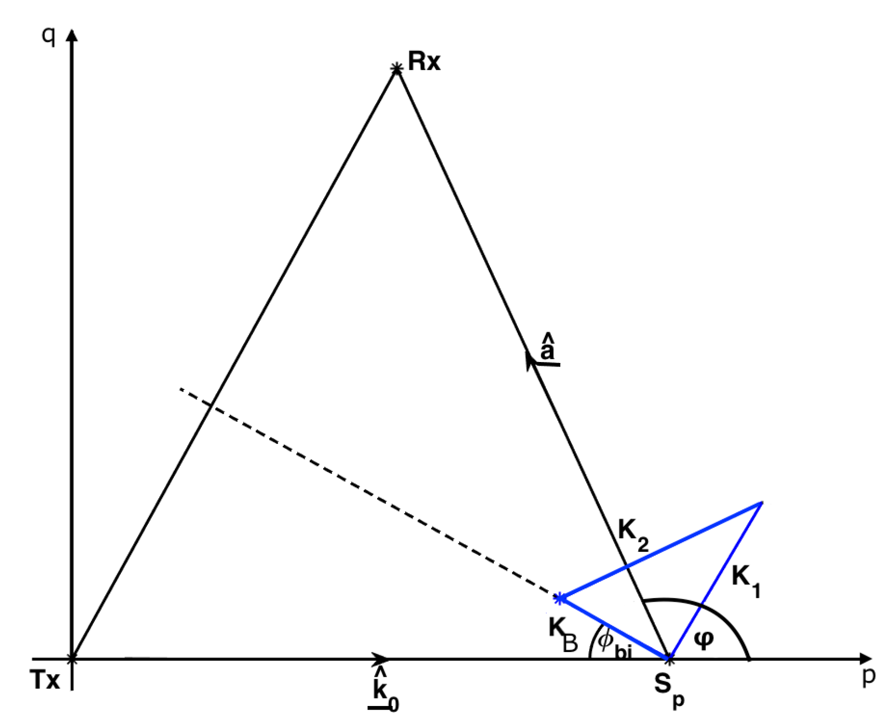
Figure 5.
Scattering geometry for a bistatic radar where , and denote the transmitter, scatter patch and receiver respectively, is the bistatic angle, is the radar wavevector and, p and q are spatial wavenumbers, with p in the direction of the emitted radio wave.
Figure 5.
Scattering geometry for a bistatic radar where , and denote the transmitter, scatter patch and receiver respectively, is the bistatic angle, is the radar wavevector and, p and q are spatial wavenumbers, with p in the direction of the emitted radio wave.

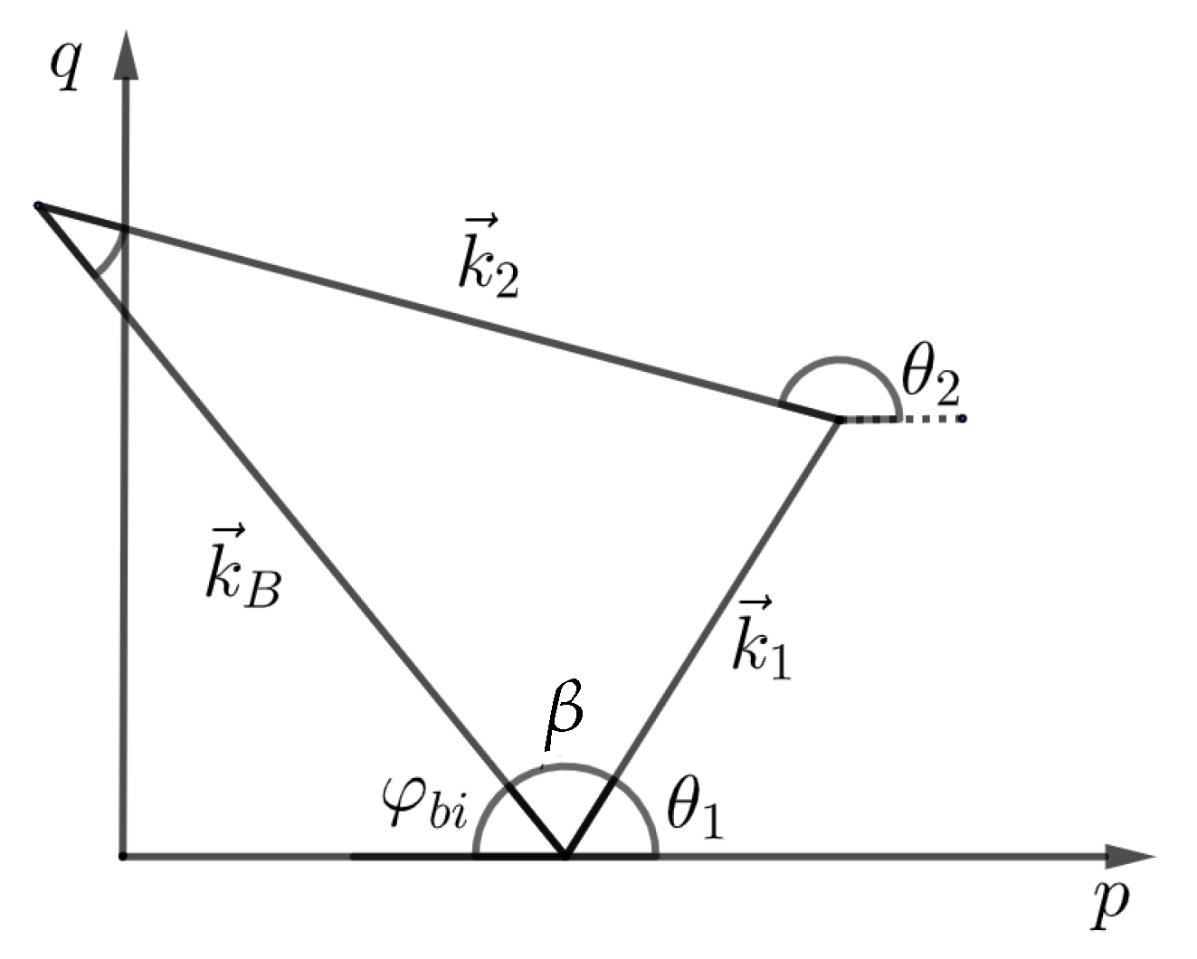
Figure 6.
Geometry of the second order scattering wave vectors, and , at angles and , respectively.

Figure 7.
The frequency contours of Equation (36) for two values of , (a) monostatic and (b) bistatic angle when . The normalised frequency, , is shown by the colour, in the p, q plane.
Figure 7.
The frequency contours of Equation (36) for two values of , (a) monostatic and (b) bistatic angle when . The normalised frequency, , is shown by the colour, in the p, q plane.

Figure 8.
The frequency contours of Equation (36) shown for (where ) with two different values for : (a) monostatic and (b) bistatic angle . The colour shows the value of the normalised frequency, , in the p, q plane.
Figure 8.
The frequency contours of Equation (36) shown for (where ) with two different values for : (a) monostatic and (b) bistatic angle . The colour shows the value of the normalised frequency, , in the p, q plane.

Figure 9.
Contours in the p, q plane defined by Equation (36) when . (a) Bistatic case with bistatic angle , (b) monostatic case. The electromagnetic singularities are shown for both monostatic and bistatic radars. The yellow dashed circle shows the singularities defined by Equation (50) and the magenta dotted circle shows those defined by Equation (51). In the monostatic case, Equations (50) and (51) are equal and hence both circles are in the same location. The white contours highlight the frequencies tangential to the circles.

Figure 10.
A simulated bistatic Doppler spectrum showing the electromagnetic singularities.

Figure 11.
Inverted data for case 1. (a) monostatic (b) 1 bistatic. Current speed and direction on left, shortwave directional spreading and wind direction, centre, significant waveheight and peak direction, right.
Figure 11.
Inverted data for case 1. (a) monostatic (b) 1 bistatic. Current speed and direction on left, shortwave directional spreading and wind direction, centre, significant waveheight and peak direction, right.

Figure 12.
Inverted data for case 2. (a) monostatic (b) 1 bistatic.

Figure 13.
Inverted swell and wind wave components for case 2 (a) monostatic (b) 1 bistatic.

Figure 14.
Inverted data for case 3. (a) monostatic (b) 1 bistatic.

Figure 15.
Inverted data for case 4. (a) monostatic (b) 1 bistatic.

Figure 16.
Inverted data for case 5. (a) monostatic (b) 1 bistatic.

Figure 17.
Inverted data for case 6. (a) monostatic (b) 1 bistatic.

Figure 18.
Inverted spectra for case 3. (a) monostatic (b) 1 bistatic.

Figure 19.
Inverted spectra for case 4. (a) monostatic (b) 1 bistatic.

Figure 20.
Inverted spectra for case 5. (a) monostatic (b) 1 bistatic.

Figure 21.
Inverted spectra for case 6. (a) monostatic (b) 1 bistatic.

Figure 22.
Scatter plots and statistics of the current measurements. These are colour-coded with the bistatic angle.
Figure 22.
Scatter plots and statistics of the current measurements. These are colour-coded with the bistatic angle.

Figure 23.
Scatter plots and statistics of the wave parameter measurements, colour-coded with the bistatic angle.
Figure 23.
Scatter plots and statistics of the wave parameter measurements, colour-coded with the bistatic angle.


Table 1.
Wave, wind and current parameters used for the Doppler spectra simulations. The buoy data are not separated into wind–waves and swell but their peak period and direction are included in the swell columns.
Table 1.
Wave, wind and current parameters used for the Doppler spectra simulations. The buoy data are not separated into wind–waves and swell but their peak period and direction are included in the swell columns.
| Case | Type | Wind–Wave Hs m | Spread | Wind Speed m/s | Current Speed m/s | Swell Hs m | Tp s | Spread | |||
|---|---|---|---|---|---|---|---|---|---|---|---|
| 1 | Model | 3.07 | 0.0 | 3.0 | 12.0 | 1.4 | 70.0 | ||||
| 2 | Model | 3.07 | 30.0 | 2.0 | 12.0 | 1.8 | 90.0 | 3.0 | 140.0 | 13.2 | 10.0 |
| 3 | Buoy | 1.72 | 1.8 | 90.0 | 68.24 | 12.8 | |||||
| 4 | Buoy | 1.72 | 1.8 | 90.0 | 148.16 | 6.74 | |||||
| 5 | Buoy | 2.70 | 1.8 | 90.0 | 109.01 | 14.22 | |||||
| 6 | Buoy | 5.87 | 1.0 | 245.0 | 162.36 | 9.85 |
Table 2.
Configuration parameters at selected cells.
| Cell Number | Configuration | Bistatic Angle | Angle between Braggs |
|---|---|---|---|
| 1664 | monostatic | 0 | 40.6 |
| 1 mono, 1 bistatic | 20.4 | 20.3 | |
| 3116 | monostatic | 0 | 60.0 |
| 1 mono, 1 bistatic | 30.1 | 29.9 | |
| 3128 | monostatic | 0 | 77.8 |
| 1 mono, 1 bistatic | 39.1 | 38.8 | |
| 3140 | monostatic | 0 | 99.6 |
| 1 mono, 1 bistatic | 50.1 | 49.5 |
© 2020 by the authors. Licensee MDPI, Basel, Switzerland. This article is an open access article distributed under the terms and conditions of the Creative Commons Attribution (CC BY) license (http://creativecommons.org/licenses/by/4.0/).
Share and Cite
MDPI and ACS Style
Hardman, R.L.; Wyatt, L.R.; Engleback, C.C. Measuring the Directional Ocean Spectrum from Simulated Bistatic HF Radar Data. Remote Sens. 2020, 12, 313. https://0-doi-org.brum.beds.ac.uk/10.3390/rs12020313
AMA Style
Hardman RL, Wyatt LR, Engleback CC. Measuring the Directional Ocean Spectrum from Simulated Bistatic HF Radar Data. Remote Sensing. 2020; 12(2):313. https://0-doi-org.brum.beds.ac.uk/10.3390/rs12020313
Chicago/Turabian StyleHardman, Rachael L., Lucy R. Wyatt, and Charles C. Engleback. 2020. "Measuring the Directional Ocean Spectrum from Simulated Bistatic HF Radar Data" Remote Sensing 12, no. 2: 313. https://0-doi-org.brum.beds.ac.uk/10.3390/rs12020313
Note that from the first issue of 2016, this journal uses article numbers instead of page numbers. See further details here.