Deep Neural Network Cloud-Type Classification (DeepCTC) Model and Its Application in Evaluating PERSIANN-CCS

Abstract

Satellite remote sensing plays a pivotal role in characterizing hydrometeorological components including cloud types and their associated precipitation. The Cloud Profiling Radar (CPR) on the Polar Orbiting CloudSat satellite has provided a unique dataset to characterize cloud types. However, data from this nadir-looking radar offers limited capability for estimating precipitation because of the narrow satellite swath coverage and low temporal frequency. We use these high-quality observations to build a Deep Neural Network Cloud-Type Classification (DeepCTC) model to estimate cloud types from multispectral data from the Advanced Baseline Imager (ABI) onboard the GOES-16 platform. The DeepCTC model is trained and tested using coincident data from both CloudSat and ABI over the CONUS region. Evaluations of DeepCTC indicate that the model performs well for a variety of cloud types including Altostratus, Altocumulus, Cumulus, Nimbostratus, Deep Convective and High clouds. However, capturing low-level clouds remains a challenge for the model. Results from simulated GOES-16 ABI imageries of the Hurricane Harvey event show a large-scale perspective of the rapid and consistent cloud-type monitoring is possible using the DeepCTC model. Additionally, assessments using half-hourly Multi-Radar/Multi-Sensor (MRMS) precipitation rate data (for Hurricane Harvey as a case study) show the ability of DeepCTC in identifying rainy clouds, including Deep Convective and Nimbostratus and their precipitation potential. We also use DeepCTC to evaluate the performance of the Precipitation Estimation from Remotely Sensed Information using Artificial Neural Networks-Cloud Classification System (PERSIANN-CCS) product over different cloud types with respect to MRMS referenced at a half-hourly time scale for July 2018. Our analysis suggests that DeepCTC provides supplementary insights into the variability of cloud types to diagnose the weakness and strength of near real-time GEO-based precipitation retrievals. With additional training and testing, we believe DeepCTC has the potential to augment the widely used PERSIANN-CCS algorithm for estimating precipitation.

1. Introduction

Clouds play a crucial role, as an element of the Earth system, in a wide range of hydrometeorological and engineering applications, yet there is not a deep understating of their physical dynamics. Satellite cloud remote sensing is pivotal in identifying meteorological conditions and hydrological components such as precipitation [1,2]. Low Earth Orbiting (LEO) satellite observations are recognized as reliable sources to characterize clouds and their associated precipitation processes but they are limited due to their narrow satellite swath and low temporal coverage characteristics. Although data retrieved from Geosynchronous Earth Orbiting (GEO) satellites are reliant solely on cloud top properties such as temperature and albedo, their high spatiotemporal and spectral resolution data stream makes them a very attractive to monitor the distribution of various cloud types. Recent developments in satellite technologies resulting in higher temporal, spatial and spectral resolutions, along with advancements in machine learning techniques and computational power, open great opportunities to develop efficient near real-time models to characterize cloud types and their behaviors.

The history of satellite-based cloud detection using infrared and visible imageries began with studies by Booth [3] and Hughes [4], followed by Goodman and Henderson-Sellers [5], Rossow [6], Rossow and Garder [7], Wielicki and Parker [8], Key [9], Yhann and Simpson [10]. Rossow and Schiffer [11] used cloud top pressure and cloud optical depth information to provide a valuable comprehensive study about global climatology of clouds, International Satellite Cloud Climatology Project (ISCCP). Several methods have been developed to classify clouds from single- or multispectral satellite imageries, including threshold-based [12,13,14,15,16] and machine learning approaches. The main drawback of threshold-based cloud-type classification (e.g., Reference [17]) is that a threshold over certain situations may not be applicable for another [18]. Also, a large number of studies have addressed satellite cloud-type classification from a variety of perspectives but they rely on specific regions. For instance, Hameg et al. [19] used a naive Bayes classifier and northern Algeria weather radar observations to find the relationship between predefined spectral parameters from MSG-SEVIRI (Meteosat Second Generation-Spinning Enhanced Visible and Infrared Imager) for convective clouds differentiation. Tebbi and Haddad [20] focused on the combination of two machine learning models and Lazri and Ameur [21] utilized an ensemble of learning algorithms to identify convective or stratiform precipitation over a small Mediterranean region. It should be pointed out that the computational expenses and complexity of the implementation of these models are challenging.

One of the primary applications of a classical machine learning methodology in cloud classification was presented by Lee et al. [22] using a single visible channel of Landsat Multispectral Scanner sensor to classify Stratocumulus, Cumulus, and Cirrus cloudy images. Yhann and Simpson [10] combined top-of-atmosphere reflectance and radiance from the National Oceanic and Atmospheric Administration’s (NOAA) Advanced Very High-Resolution Radiometer (AVHRR) to detect cloudy pixels. Bankert [23] and Tian et al. [24] investigated the performance of neural-network-based cloud classifications on AVHRR measurements and multispectral GOES-8 satellite imagery, respectively. Cloud Automated Neural Network (CANN) was presented by Miller and Emery [25] which defined different thresholds along with six textural features to distinguish between nine cloud classes. Hsu et al. [26] used the Self-Organizing Feature Map (SOFM) to classify cloud features into several groups in the Precipitation Estimation from Remotely Sensed Information using Artificial Neural Networks algorithm (PERSIANN) [27]. Mazzoni et al. [28] used a Support Vector Machine (SVM) cloud-type classifier on NASA’s Terra satellite measurements. Nasrollahi [29] developed an artificial neural network cloud classification system using CloudSat and MODIS datasets. Also, Cai and Wang [30] and Wohlfarth et al. [31] applied SVM and neural network cloud classification algorithms on Fy-2C and Landsat8 images, respectively.

Both supervised (classification) (e.g., Reference [32]) and unsupervised learning (clustering) (e.g., Reference [33]) techniques have helped in analyzing the large amount of real-time remotely sensed data (i.e., Big Data) and have proven their abilities to discriminate different cloud characteristics. Supervised neural networks classifiers are flexible and fast in learning [34] and they reveal their capability of dealing with consecutive images from GEO satellites with promising results for meteorological application [24,31,35]. In recent years, deep learning algorithms have been a popular solution to overcome the complexity of real-time data mining problems in earth and atmospheric sciences. Ball et al. [36] reviewed the existing deep learning methods and discussed the advantages of applying these techniques in remote sensing science. Tao et al. [37] presented a related application of deep learning techniques to generate binary classification (i.e., rain/no-rain pixels). They showed the effectiveness of using water vapor and infrared data in deep neural network models which aid in capturing rainy clouds. However, this research does not attempt to conduct any information of cloud types and their precipitation potentials.

The purpose of this study is to take advantage of revolutionized Cloud Profiling Radar (CPR) on National Aeronautics and Space Administration’s (NASA) CloudSat satellite and the new generation of GEO-based sensors such as the Advanced Baseline Imager (ABI) onboard GOES-16/17 satellites to develop a near real-time global-scale cloud-type classification system. The output would serve as a valuable real-time source of data for hydrometeorological applications as well as improving rain detection skills in GEO-based precipitation retrievals such as Precipitation Estimation from Remotely Sensed Information Using Artificial Neural Networks-Cloud Classification System (PERSIANN-CCS) [16]. This effort will support the current NASA Integrated Multisatellite Retrievals for Global Precipitation Measurement (IMERG) system [38], which unifies multiple algorithms such as PERSIANN-CCS and Climate Prediction Center Morphing with Kalman Filter (CMORPH-KF) [39].

PERSIANN-CCS uses an incremental temperature threshold approach for cloud-patch segmentation and then employs an unsupervised classification technique to differentiate between cloud patches based on similarity of statistical indices (i.e., features). These features are predefined to capture coldness, geometry, and texture properties of the clouds with little attention to distinguish between the cloud types such as Nimbostratus, Cumulus, Altocumulus, or Deep Convective clouds before rainfall mapping. Deep Convective clouds produce higher rain rates (convective rainfall) compared to Nimbostratus clouds (stratiform rainfall). It is possible that Cumulus congestus clouds produce drizzle but they can grow into Cumulonimbus clouds associated with heavy rain. Clearly, limited features are insufficient to interpret actual cloud types. Therefore, establishing rapid cloud-type classification will provide supplementary insights into the variability of the vertical structure of clouds, stages of a cloud’s life cycle, and their associated precipitation systems [29,40].

Our contributions in this paper are summarized as:

(1)

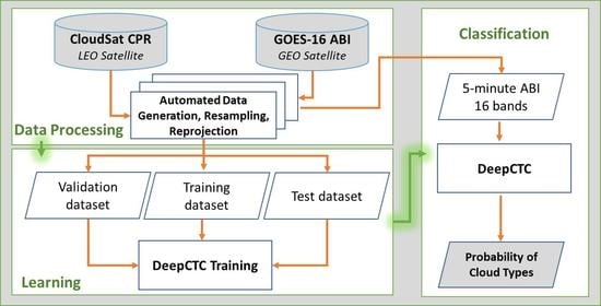
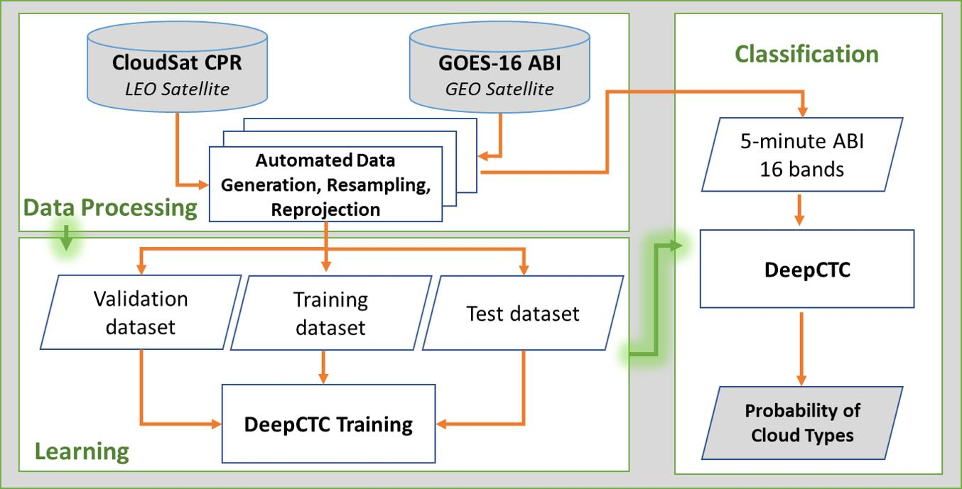
Introducing an automatic data generation pipeline to meet the critical demand for an accurately labeled cloud-type dataset. The integration of CloudSat space-borne radar satellite data with GOES-16 ABI observations also addresses the spatial and temporal discontinuity in cloud-type information from narrow satellite swaths.

(2)

Using the Deep Neural Network Cloud-Type Classification (DeepCTC) system to perform a rapid and global cloud-type classification for the new generation of geostationary satellite observations (e.g., GOES-16 ABI).

(3)

Evaluating the performance of PERSIANN-CCS based on DeepCTC to diagnose the weakness and strength of precipitation estimates over different cloud types. This assessment is performed over a period of one month (July 2018) for half-hourly precipitation estimates.

The rest of this paper is organized as follows: Section 2 describes the data sets and domain used in this study. In Section 3, the methodology and general workflow of DeepCTC are reported. Results and discussions are provided in Section 4. Lastly, Section offers Section 5 the conclusion and future direction of DeepCTC. In the rest of the paper, to be consistent in the terminology, “classification” refers to supervised machine learning techniques which assign single pixels from multispectral imageries to different classes [41].

2. Data Sources

2.1. CloudSat

The unique NASA CloudSat CPR is a 94 GHz (3.2 mm) nadir-looking radar, providing a valuable source of information about the vertical properties of clouds [42]. The nominal vertical resolution is about 480 m and the horizontal resolution is about 1.4 km and 1.7 km across and along the track, respectively. In this study, CloudSat Level 2 Cloud Scenario Classification product (2B-CLDCLASS) [1] is used to train, validate and test the DeepCTC model (from 2017 to present). The widely used 2B-CLDCLASS product integrates passive remote sensing data from MODIS (including bands 0.6, 0.8, 1.3, 8.5, 11 and 12 $\mathsf{\mu }$m), CPR and CALIPSO lidar measurements. Based on different rules for the vertical and horizontal extent of hydrometeors, the maximum radar reflectivity factor, indications of precipitation and ancillary data including predicted European Center for Medium-Range Weather Forecast (ECMWF) temperature profiles and surface topography height, 2B-CLDCLASS provides most, but not all, tropospheric cloud types. Some studies show the consistency of cloud-type information from this product with ISCCP data [43], cloud water content [44], and precipitation occurrence [45]. The 2B-CLDCLASS process description is available at http://www.cloudsat.cira.colostate.edu/data-products/level-2b/2b-cldclass?term=88.

Table 1. Characteristics of cloud types.

	Cloud-Type	Vertical Dimension	Cloud Base Level	Precipitation	Horizontal Dimension
1	High clouds (Hi)	Moderate	High	None	Continuous
2	Altostratus (As)	Moderate	Middle	None	Continuous
3	Altocumulus (Ac)	Shallow/ Moderate	Middle	None/Drizzle	Discontinuous
4	Stratus (St)	Shallow/ Moderate	Low	Possible	Continuous
5	Stratocumulus (Sc)	Shallow	Low	Possible	Discontinuous
6	Cumulus (Cu)	Moderate/ Deep	Low	Possible	Isolated
7	Nimbostratus (Ns)	Deep	Low/ Middle	Yes	Continuous
8	Deep Convective (DC)	Deep	Low	Yes	Continuous

presents a brief listing of the cloud types which will be used in this study [1]. The High cloud types include Cirrus, Cirrocumulus and Cirrostratus which are thin in horizontal direction and are predominantly non-rainy clouds with cold cloud-top temperature in IR images. The Cumulus cloud-type is Cumulus Congestus and fair weather Cumulus in lower part of the atmosphere with flat bases. Cumulus clouds are expanded vertically and they can turn into Cumulonimbus clouds in less than 30 min. Deep Convective and Nimbostratus cloud types are mainly precipitable clouds which expand from the lower level of the atmosphere to the higher troposphere; Deep Convective clouds result in higher precipitation intensity than the Nimbostratus type [1,43,46,47].

2.2. Geostationary Satellite Observations

For this study, Level 2 Cloud and Moisture Imagery Product (CMIP) from the Advanced Baseline Imager (ABI) onboard the GOES-R series of NOAA geostationary meteorological/environmental satellite (GOES-16) is used. The proposed algorithm is flexible to be extended to other GEO-based observations including GOES-17 ABI and Himawari 8/9 AHI. GOES-16 scans the full disk western hemisphere every 15 min and Continental United States (CONUS) every 5 min on the “flex” mode. GOES-16 ABI measures reflected and emitted radiance in two bands at visible wavelengths (0.47 and 0.64 $\mathsf{\mu }$m central), four near-infrared bands (0.86, 1.37, 1.6 and 2.2 $\mathsf{\mu }$m central) and ten bands at thermal infrared with approximate central wavelengths of 3.9, 6.2, 6.9, 7.3, 8.4, 9.6, 10.3, 11.2, 12.3 and 13.3 $\mathsf{\mu }$m [48]. Additional information about GOES-16 ABI sensors are described in

Table 2. Properties of ABI bands.

ABI Bands	Descriptive Name	Central Wavelength	Primary Purpose
1	Blue	0.47 $\mathsf{\mu }$m	Aerosol monitoring
2	Red	0.64 $\mathsf{\mu }$m	Detection of smoke, dust, fog and low level clouds
3	Vegetation	0.86 $\mathsf{\mu }$m	Aerosol and cloud monitoring; Land characterizing (NDVI)
4	Cirrus	1.37 $\mathsf{\mu }$m	Daytime detection of thin/high cirrus clouds
5	Snow/Ice	1.61 $\mathsf{\mu }$m	Snow and ice discrimination, Cloud phase detection
6	Cloud particle size	2.24 $\mathsf{\mu }$m	Cloud particle size and cloud phase discrimination
7	Shortwave window	3.9 $\mathsf{\mu }$m	Fog, low level and stratus cloud identification
8	Upper-level water vapor	6.19 $\mathsf{\mu }$m	Tropospheric water vapor monitoring
9	Middle-level water vapor	6.93 $\mathsf{\mu }$m	Tropospheric water vapor monitoring
10	Lower-level water vapor	7.37 $\mathsf{\mu }$m	Tropospheric water vapor monitoring
11	Cloud top phase	8.44 $\mathsf{\mu }$m	Determining cloud phase
12	Ozone	9.61 $\mathsf{\mu }$m	Dynamics of the atmosphere near tropopause
13	Clean long-wave window	10.33 $\mathsf{\mu }$m	Cloud boundary detection
14	Long-wave window	11.21 $\mathsf{\mu }$m	Cloud boundary detection
15	Dirty long-wave window	12.29 $\mathsf{\mu }$m	Distinguishing dust and volcanic ash from clouds
16	CO2	13.28 $\mathsf{\mu }$m	Cloud top height

. ABI can monitor multiple layers of the Earth-atmosphere system with a wide range of imagery and radiometric information related to cloud products (chap. 4 and 6 [49]). The nominal spatial resolution at the sub satellite pixel is 0.5 km for the “Red” band, 1 km for “Blue”, “Vegetation”, “Snow/Ice” bands and 2 km for other thermal emissive bands. ABI data implemented in our experiments are resampled (bilinear interpolation) to ${0.01}^{°}$ spatial resolution.

A theoretical description of the algorithms used by CMIP can be found in the Algorithm Theoretical Basis Document by Schmit et al. [50]. The GOES-16 ABI data (from 2017 to present) is available for public access through the NOAA’s comprehensive Large Array-data Stewardship System (CLASS) at https://www.avl.class.noaa.gov/saa/products/welcome. In this study, we use NOAA’s GOES-16 ABI data on Amazon Web Services (AWS) S3 bucket (https://registry.opendata.aws/noaa-goes/). Using the AWS S3 Command Line Interface (CLI), a list of all available files in the S3 bucket is created. This list is used to look up time based GOES-16 ABI files in the automated data generation pipeline which is explained in Section 3.2.

2.3. Precipitation Datasets

NOAA/National Severe Storms Laboratory—University of Oklahoma Level-3 half-hourly gauge-adjusted Multi-Radar Multi-Sensor (MRMS) [51] product at 0.01${}^{°}$ resolution is used to examine the performance of the proposed cloud-type classification model and PERSIANN-CCS product. This high-resolution quality-controlled rain rate mosaic covers an area with latitude bounds of 20${}^{°}$ and 55${}^{°}$N and longitude bounds of 130${}^{°}$ and 60${}^{°}$W, available from 1 June 2014 (http://wallops-prf.gsfc.nasa.gov/NMQ/index.html). Level-3 half-hourly MRMS is liquid precipitation and 0.1 mm/h rain rate was used as a threshold to define rain/no-rain pixels. In order to show high variability of cloud types and different rainfall pattern during one day, Hurricane Harvey which caused extreme precipitation [52] during 26–28 August 2017 is considered as a case study. Both GOES-16 and CloudSat satellites completely monitored this event on 26 August and MRMS rain rates provides independent data for assessing cloud types covering different precipitation patterns.

The half-hourly MRMS rain rate dataset is mapped to 0.04${}^{°}$ spatial resolution to evaluate PERSIANN-CCS product over the CONUS for July 2018. The operational near real-time high resolution (0.04${}^{°}$) PERSIANN-CCS product is developed by the Center for Hydrometeorology and Remote Sensing (CHRS) at the University of California, Irvine (UCI) and is available through the CHRS Data Portal (http://chrsdata.eng.uci.edu/). As mention earlier, this algorithm uses solely infrared satellite imagery to map rain rate in near global- scale and details about this product can be found in [16,26].

3. Methodology

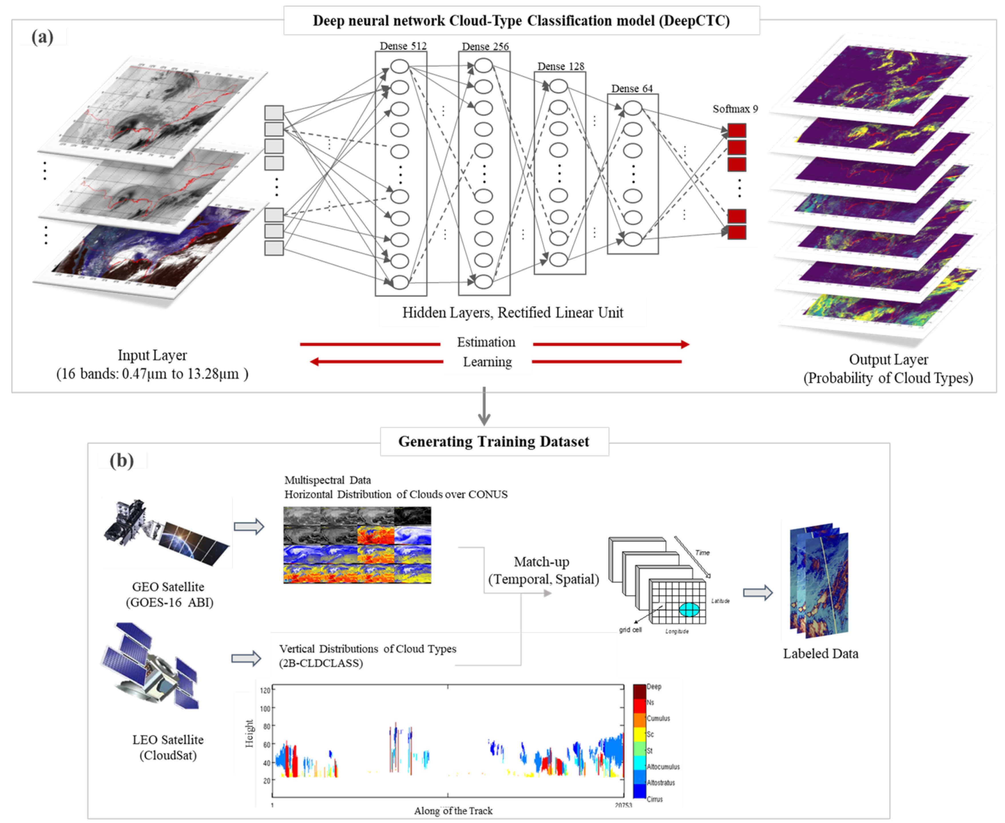
3.1. The Architecture and Configuration of DeepCTC

The Deep Neural Network Cloud-Type Classification (DeepCTC) model is a multilayer perceptron classification system which includes successive layers. Each layer composed of several neurons that receive outputs from preceding layers by weighted connections. As shown in Figure 1a DeepCTC consists of one input layer taking a series of normalized values from visible, water vapor and infrared observations from GOES-16 ABI (16 neurons), 4 sequential fully connected hidden layers and one output layer (9 neurons). For the node j in the kth hidden layer, the net input $x_{kj}$ is a weighted average of the outputs of the $(k-1)$th layer which is given by:

$$x_{kj}=\sum _{i=1}^{N_{k-1}}{w}_{(k-1)ij}{O}_{(k-1)i}, \mathrm{where} O_{kj}=max(0,x_{kj}).$$

(1)

$w_{(k-1)ij}$ is the synapse coefficient of the node i in the $(k-1)$th layer to the node j in the kth. $N_k$ is the number of nodes in the kth layer and $O_{kj}$ is the output of node j in the kth hidden layer which is computed by Rectified Linear Unit activation function (ReLU). We used ReLU in our backpropagation model to speed up the training procedure with more accurate results [53]. The last layer, maps the non-normalized output of the deep neural network to a probability distribution over possible cloud labels. The activation function in this layer is a normalized exponential function (Softmax) defined by the following expression:

$$P(y=c|\xi )=\frac{exp({\xi }^{T}W+b)}{{\sum }_{c=1}^{C}exp({\xi }^{T}W+b)}.$$

(2)

$\xi$ and W are output (labeled) and weight vectors of penultimate layer, respectively. ${\xi }^T$ is the transpose of matrix $\xi$; b is bias vector of the cth cloud class and C is the total number of classes. We used the Adam optimizer to train the deep neural network and minimize the loss function (Equation (3)); Adam is well suited for non-stationary objectives and noisy gradients [54]. The categorical cross entropy loss function (Adam) represents the dissimilarity of the approximated output distribution from the true labels given by:

$$\mathcal{L}=-i/N\sum _{c=1}^C{Y}_{c}ln{y}_c;$$

(3)

where the $Y_c$ is a vector of cth class and $y_c$ is vector of predicted categories [55]. To mitigate the overfitting issue and improve the performance of the network, DeepCTC is regularized with a 0.1 dropout rate to hidden layers [56].

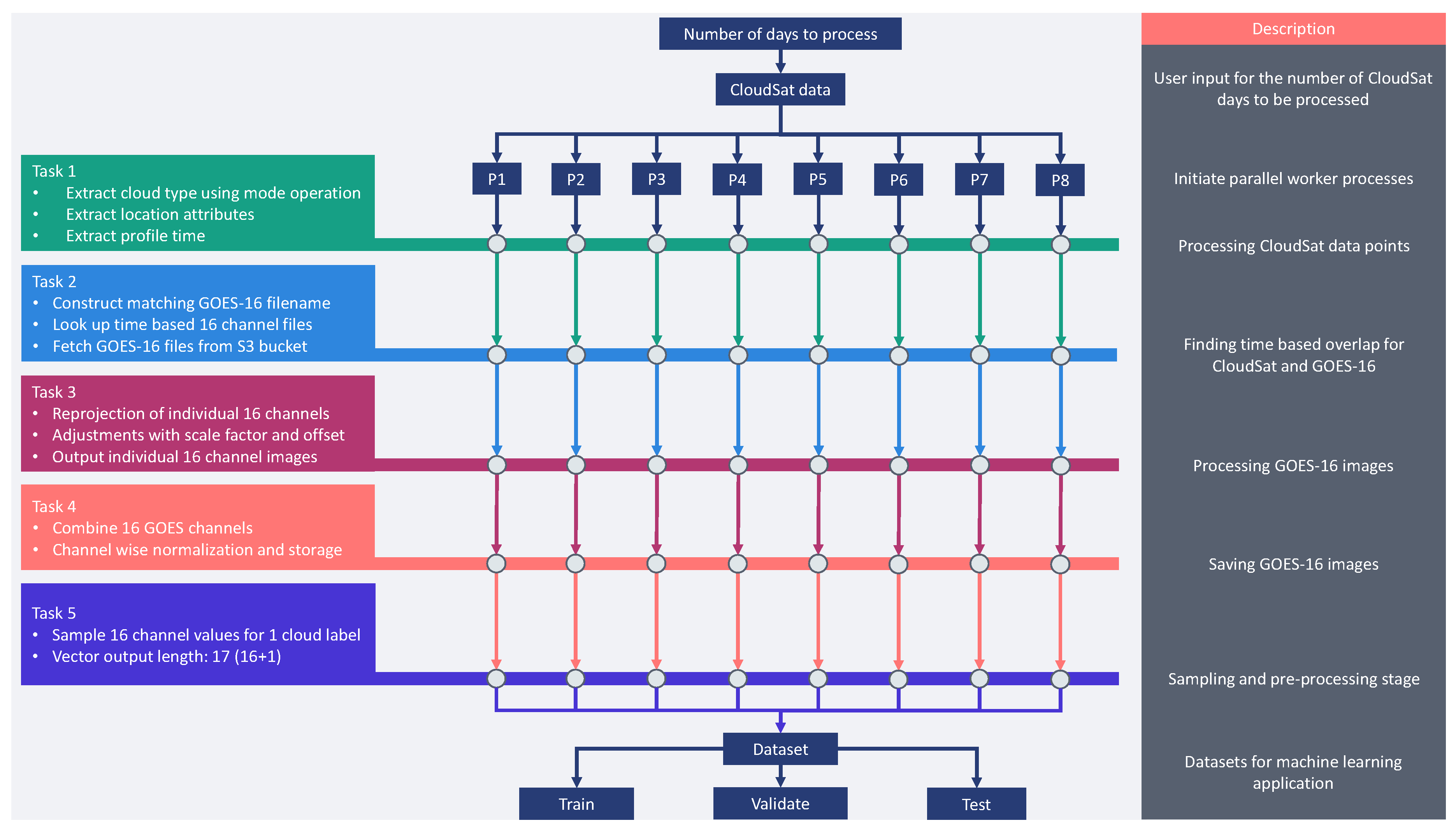
3.2. Automated Data Generation Pipeline

Providing large, labeled and scientific datasets is one of the most challenging parts of the supervised deep learning cloud-type classification approach [57]. In most real-time cloud-type classification studies, limited human-reported datasets are used which rely on experts’ experience. The unreliability of these datasets stems from their dependency on manual interpretations and introduces concealed uncertainty in classification results. In this study, we met the critical demand for a large, accurately labeled dataset concerning the different types of clouds. An automatic data processing pipeline is implemented to generate multi-class data from coincidences of LEO-based CloudSat observations and multispectral GEO-based imagery (Figure 1b). One of the benefits of this extendable scheme is that it can be applied to the new generation of advanced GEO satellites with similar channels and capabilities such as ABI on GOES-16/17, Advanced Himawari Imager (AHI) on Himawari-8/9, Advanced Meteorological Imager (AMI) on GEO-KOMPSAT2A, Flexible Combined Imager (FCI) on Meteosat Third Generation-Imaging (MTG-I) and Advanced Geosynchronous Radiation Imager (AGRI) on Fengyun-4A. Also, using vertical properties of clouds from the CloudSat satellite, which is nearing the end of its expected lifetime, is a pioneering effort to be followed by the Earth Clouds, Aerosol and Radiation Explorer (EarthCARE) mission [58]. Another advantage of training this deep neural network classification model with reliable and large datasets is the “Transfer Learning” capability; this trained model can be reused in related investigations [59].

The experimental cloud-type dataset is prepared for all available CloudSat 2B-CLDCLASS data coincident with GOES-16 ABI observations (CMIP) for 2017 within the bounds of the case study (CONUS). We achieve this goal by creating an automated data generation pipeline which requires minimum user involvement. A user simply defines the total number of CloudSat days to be processed and the training data for DeepCTC model is generated automatically. The key major steps in the automated data generation pipeline includes: finding the cloud types, searching the appropriate time based GOES-16 ABI files within a time window, obtaining and pre-processing the 16 bands, generating multispectral images and finally sampling cloud labels. To speed-up the overall procedure when handling the high volume of GOES-16 data, parallel processes are utilized which works independently by processing an individual CloudSat 2B-CLDCLASS data point. The overall procedure for processing one point using a single process is explained with the help of a task based schematic as shown in Figure 2.

The key information such as location attributes (latitude and longitude) and the time of the bins are extracted from a given 2B-CLDCLASS profile. A mode operation is carried out on the bins to identify cloud types that appear the most frequently. The profile time is used to identify the required GOES-16 ABI images within a specified 30-second time window since each CloudSat profile represents 160 milliseconds of time and 1.1 km of distance for one horizontal pixel [60]. The S3 bucket download links for the identified GOES-16 ABI files are looked up from an indexed file containing all the S3 bucket GOES-16 download links. The individual files are downloaded automatically and processed further for re-projection, scaling pixel values and adding offsets. All 16 bands are combined to create a single multispectral image (${0.01}^{°}$ spatial resolution) which gets cropped for the CONUS and is stored to the disk after carrying out a band wise normalization pre-processing operation. The location attributes of the cloud-type are used to sample a vector (length 16) from the stored multispectral image. Finally, the vector containing the multispectral data along with the cloud-type label provides a single entry of the dataset. Several vectors are obtained in parallel by multiple processes which completes the dataset used in this work.

Once the dataset is ready for the machine learning application, a uniform distribution of cloud types (same number of classes) is considered in order to avoid class imbalance [29,61]. To perform an independent evaluation, the data from 26 August 2017 to 28 August 2017 along with 120,000 random samples (1500 samples from each class) are separated for testing purposes. The remaining $80\%$ of the data was randomly selected for training and $20\%$ of the data was used for validation. As described by Sassen and Wang [43], identifying the difference between Stratus and Stratocumulus clouds is challenging for the CloudSat 2B-CLDCLASS algorithm, so we consider these two middle-level cloud types in one class. To generate the labeled dataset and DeepCTC implementation, the following system configuration is used: 2 Intel CPUs each having 48 cores, 128 GB system RAM and 1 NVIDIA Quadro P6000 GPU. The implementation of DeepCTC is carried out in Python (3.6), using Keras (2.1.6) with TensorFlow (1.9.0) backend. With respect to our experimental system setup, DeepCTC is able to identify cloud types every 5 min over the study area (CONUS).

4. Results and Discussion

In order to assess the performance of the DeepCTC model, common statistical verification indices for multi-class classification models are reported; then some sample cloud-type results from GOES-16 ABI imageries during Hurricane Harvey are illustrated over the CONUS. All of the comparisons cover the test datasets (not including in the training dataset) and are based upon matching data pairs between GOES-16 and CloudSat with a spatial resolution of ${0.01}^{°}$. The MRMS half-hourly rain rate dataset is used as reference precipitation information to evaluate the ability of DeepCTC to identify different patterns of rain rates regarding cloud-type information. Furthermore, DeepCTC is used to examine the performance of high spatiotemporal resolution satellite precipitation estimates, PERSIANN-CCS, based on individual cloud types.

First, the confusion matrix is prepared with respect to the completely independent test dataset (

Table 3. Confusion matrix ($\sim \mathrm{12,000}$ total test samples).

	Predicted Cloud-Type (DeepCTC)
		Hi	As	Ac	St, Sc	Cu	Ns	Dc	No Cloud
Reference (CloudSat)	Hi	1239	46	33	8	2	1	10	161
	As	53	1317	40	13	9	1	55	9
	Ac	39	44	1182	83	22	4	27	99
	St, Sc	51	7	33	968	16	0	2	417
	Cu	43	44	71	218	998	6	14	112
	Ns	35	70	38	2	9	1312	34	0
	DC	23	76	23	13	10	22	1329	4
	No Cloud	39	2	4	47	0	0	0	1408

). This cross-tabulation provides brief information on predicted cloud types (DeepCTC) against the reference data (CloudSat 2B-CLDCLASS) (described in Appendix A). By comparing cloud-type results to the CloudSat 2B-CLDCLASS data, we can see the highest confusion is between the class of Stratus/Stratocmulus (actual) cloud types and No Cloud class (predicted), which is about $27\%$ of Stratus/Stratocmulus sample data. Also, about 15% of Cumulus clouds are miscategorized as Stratus and Stratocmulus types. These confusions confirm the difficulty of visible- and infrared-based classification models in recognizing shallow/low level clouds (see the Table 1 for more detailed information on cloud types). Note that DeepCTC model performs very well in capturing warm clouds compared to previous studies such as Nasrollahi [29]. Moreover, the model shows its capability in recognizing the difference between Deep Convective and Nimbostratus cloud types.

The common statistical indices for evaluation of a multi-class classification model are shown in

Table 4. Results for statistical evaluation of DeepCTC.

	Cloud Type
Index	Hi	As	Ac	St, Sc	Cu	Ns	DC	No Cloud
PPV	0.81	0.82	0.83	0.71	0.93	0.97	0.90	0.63
TPR	0.82	0.87	0.78	0.64	0.66	0.87	0.88	0.93
TNR	0.97	0.97	0.97	0.96	0.99	0.99	0.98	0.92
NPV	0.97	0.98	0.96	0.95	0.95	0.98	0.98	0.99
FPR	0.02	0.02	0.02	0.03	0.00	0.00	0.01	0.07

for each cloud type; these indices are described in Appendix A. In terms of TNR and NPV, DeepCTC performs very well by correctly identifying all cloud types. The probability of true negative (NPV) is more than 95% for all classes and the TNR index which indicates the specificity of predicted cloud-type is high, especially for cloud type Cu (cumulus Congestus and fair weather cumulus) and Ns (Nimbostratus). The values of PPV in Table 4 demonstrate the good agreement between predicted cloud types and the CloudSat reference data. The precision is also high for cloud types Cu and Ns, about 93% and 97%, respectively. However, we can see lower skill in the No Cloud class because of the high confusion in capturing shallow clouds (see Table 3). The high value of TPR shows the recall or effectiveness of DeepCTC in identifying cloud types, which is about 93% for the No Cloud class. Furthermore, false alarm ratio is significantly low for all cloud types (less than 0.03) and 0.07 for the No Cloud class.

In general, the average accuracy of the DeepCTC model is approximately $85\%$. It can be argued that DeepCTC is notably skillful in classifying High clouds, Altostratus, Altocumulus, Cumulus, Nimbostratus and Deep Convective Clouds but it is less accurate in the case of Stratus and Stratocumulus clouds. This mainly results from the expected confusion between low level clouds and clear sky, especially in high altitude regions in which the elevation of clouds may be at the same elevation as the surface.

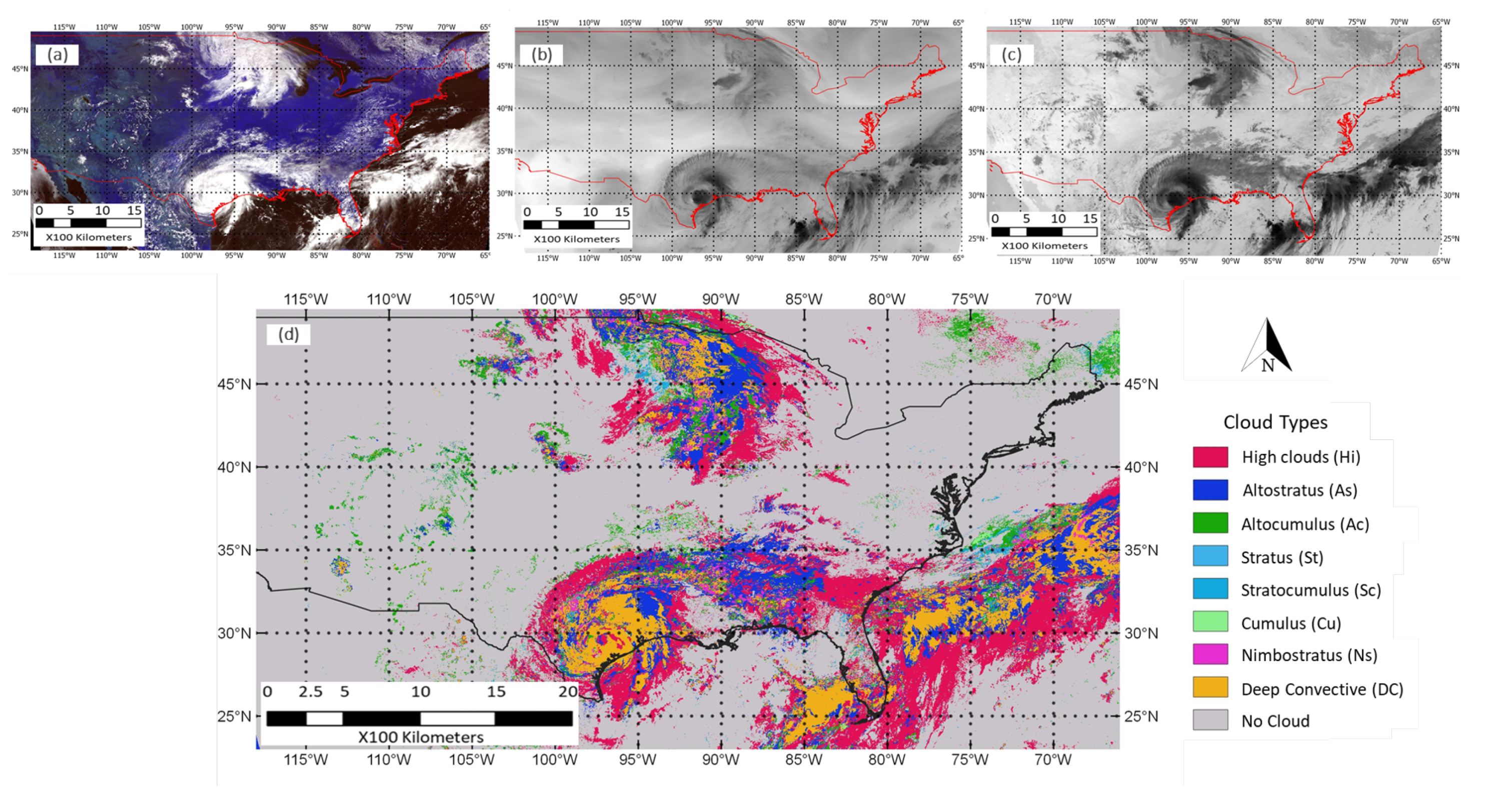
4.1. Visualization of Cloud-Type Information over the CONUS

Hurricane Harvey is chosen as a case study to illustrate the life cycle of different cloud types. Figure 3a–c displays samples from ABI’s 16 bands (0.47 to 13.28 $\mathsf{\mu }$m) as DeepCTC inputs on 26 August 2017 at 17:30 UTC and the simulated cloud types from DeepCTC are shown in Figure 3d. We take the argument of the maxima from the probability of cloud types (Softmax outputs) at each pixel to obtain the distribution of different classes (Figure 3d). This figure illustrates the Deep Convective, Altostratus and High cloud types over the southern area of Texas, the Gulf of Mexico and East Coast instantaneously with detecting the Altocumulus clouds over the central US on 26 August 2017 at 17:30 UTC. The proposed high resolution automated DeepCTC system provides a large-scale perspective of cloud types and meets the need for rapid and consistent cloud-type tracking over the CONUS and the future extension of the model to the globe.

Since DeepCTC simulates consecutive images, 288 frames per day over the CONUS, we select four random DeepCTC results during one day (26 August 2017) to demonstrate high variability and changes of cloud types during that day (Figure 4). We can see the clouds are mainly Deep Convective within the hurricane; high level clouds spiral “anticyclonically outward” and low level clouds move “cyclonically inward”, as time passes from panel a to d in Figure 4 (chap. 10 [47]). The spatial distribution of the MRMS precipitation rate within the bounds of these clouds (Figure 4e–h) shows similar motions and exhibits a strong relation between cloud types and rainy regions.

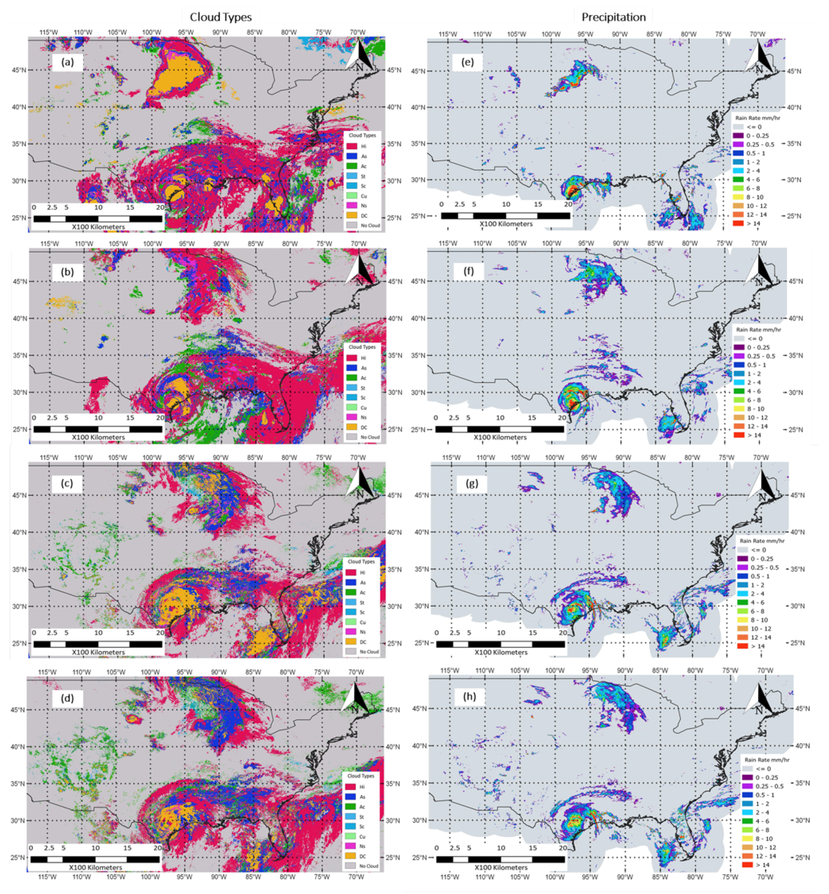
4.2. Assessment of DeepCTC Through Precipitation

The outputs of DeepCTC over the CONUS allow the exploration of spatial distribution of rainfall for various cloud types. Figure 5 displays the distinctive variation of rain rates within retrieved cloud types from DeepCTC. MRMS rain rates are 30-minute accumulated values (e.g., from 17:30 to 18:00 UTC) and cloud types in pixels are the most frequent cloud types in the same 30 min time interval. The comparison is from 0 to 10 mm/h of rain intensity on 26 August 2017. Some of the rain intensities extend to higher values but are truncated here to better represent the variability between the classes. The bin size of histograms are 0.2 mm/h and each plot shows the relative frequencies greater than a minimum 0.001 for rainfall information. A large amount of precipitation can be observed across cloud types Ns and DC, which is compatible with the observations in Figure 4. It should be mentioned that Altostratus clouds are composed of water droplets and ice crystals and they do not produce significant precipitation at the surface. However, these clouds occasionally alter to either Stratus clouds (low rain rate may occur) or Nimbostratus clouds (causes stratiform precipitation) [47]. The histogram in Figure 5b accounts for these instantaneous cloud conversions. Changes in the spatial patterns of precipitation can be seen in Figure 4.

Further details for distribution of rain rates over Deep Convective and Nimbostratus clouds are shown in Figure 6. Deep Convective and Nimbostratus clouds mostly cover extreme rainfall intensities which is consistent with the definition of these cloud types. Deep Convective clouds produce high rain rates (0.1 mm/h to about 18 mm/h) where rain drops melted from large ice particles above the freezing level are known as convective precipitation (Figure 6b).

These clouds are often surrounded spatially by Nimbostratus clouds (see Figure 4a–d). Moreover, stratiform rainfall, which results from Nimbostratus clouds, shows lower precipitation rates (0.1 mm/h to about 7 mm/h in Figure 6a) compared to that from Convective clouds (0.1 mm/h to about 18 mm/h in Figure 6b). Also, the maximum density for Nimbostratus and Deep Convective clouds are 0.65 and 0.37 in about 0.5 mm/h and 1.5 mm/h rain rates, respectively. Our comparison between different cloud types and precipitation rates is a good evidence of DeepCTC’s ability for real-time global-scale cloud-type classification and identification of their associated precipitation potential.

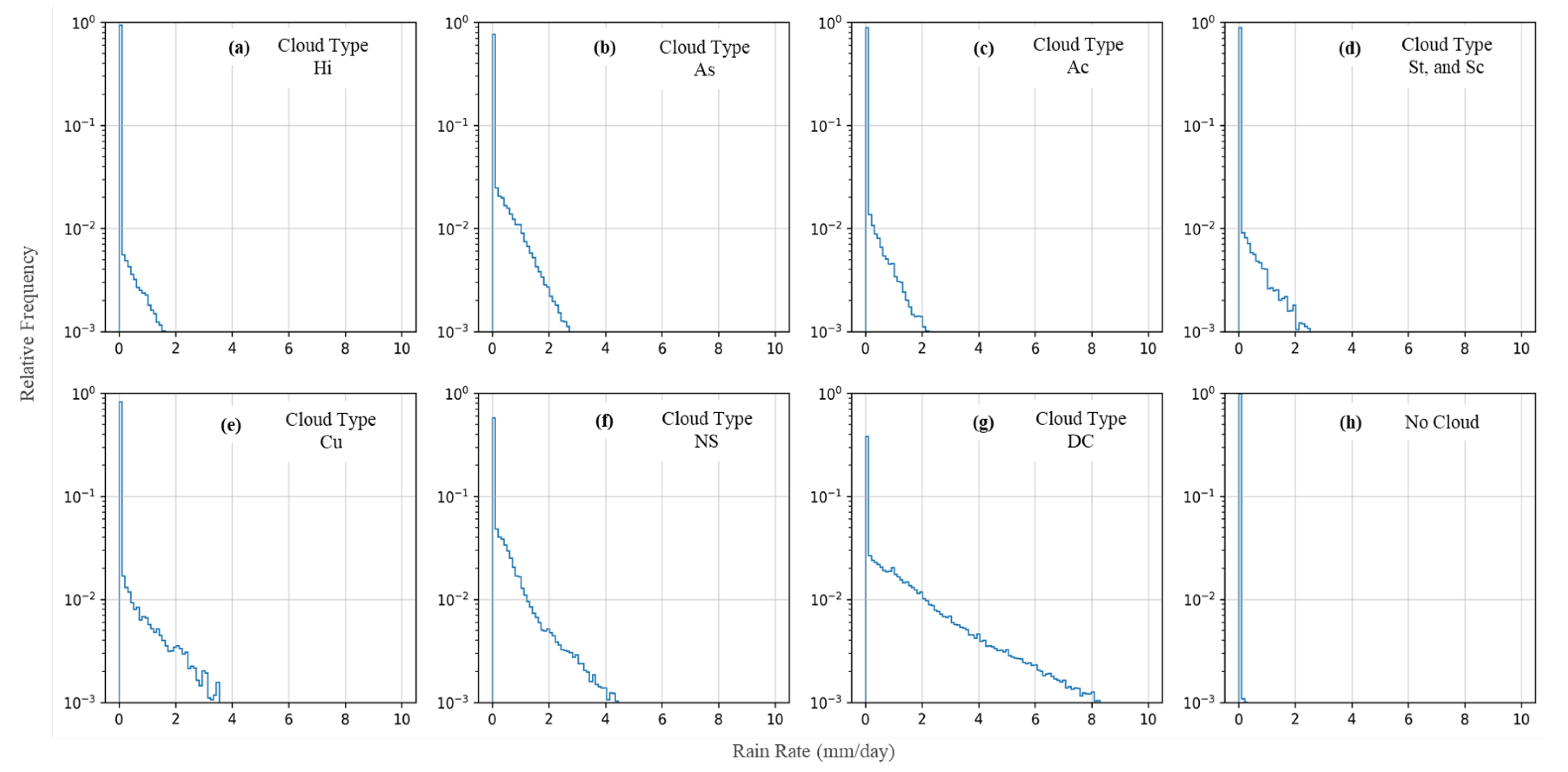
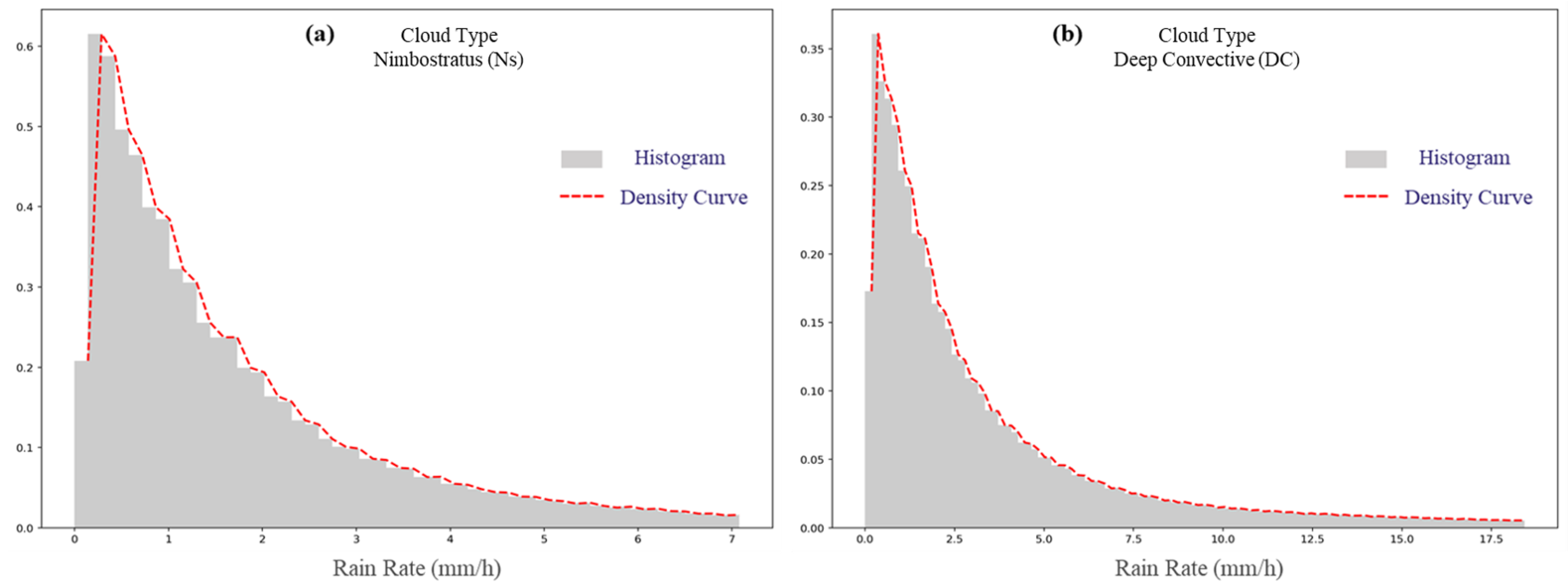
4.3. Evaluation of Half-Hourly PERSIANN-CCS According to Cloud-Type Information

We used the proposed DeepCTC model to evaluate the performance of the operational PERSIANN-CCS product based on different cloud types with respect to MRMS rain rate data as a reference, at a half-hourly scale over the CONUS. Both the MRMS and DeepCTC datasets are resampled to ${0.04}^{°}$ for each 30 min to be comparable with the PERSIANN-CCS product [62].

Table 5. Evaluation of PERSIANN-CCS across the United States for July 2018; $MRMS$ dataset is used as a reference.

	Cloud Type
Metrics	Hi	As	Ac	St, Sc	Cu	Ns	DC
$Bias$	0.69	1.19	0.32	0.70	0.39	0.82	1.56
$RMSE$$(mm/h)$	2.14	2.63	1.28	1.44	2.03	3.08	5.61
$Corr$	0.26	0.27	0.17	0.36	0.22	0.17	0.26

provides the verification statistics including Pearson correlation coefficient (Corr), bias ratio (bias) and root mean square error (RMSE) of the satellite-based precipitation estimates compared to MRMS for individual cloud types for July 2018. These continuous verification metrics are explained in Appendix A. The bias values show that PERSIANN-CCS underestimates about 65% of precipitation ratesfor cloud-type Ac. This cloud-type also has the lowest RMSE value and lowest correlation with reference data. Precipitation retrievals for cloud types Ac and Ns (with bias ratios of 1.19 and 0.82) are significantly better than other cloud types. However, PERSIANN-CCS overestimates rain rates by over 65% for High clouds (Hi). The best correlation can be seen over cloud type St, Sc with a low RMSE value of about 1.4 mm/h. The highest RMSE is associated with cloud-type DC, about 5.6 mm/h (which are the deep convective clouds with mostly high rain rates).

We examine the performance of PERSIANN-CCS with reference to MRMS data utilizing volumetric categorical indices [63] such as Volumetric Hit Index (VHI), Volumetric False Alarm Ratio (VFAR) and Volumetric Critical Success Index (VCSI) in addition to Probability of Detection (POD), False Alarm Ratio (FAR) and Critical Success Index (CSI). These categorical metrics are explained in Appendix A. Figure 7 displays the summary of volumetric indices for each cloud-type for evaluating the entire distribution of precipitation estimation with a 0.1 mm/h rain rate threshold for July 2018 over the CONUS. Notice that 1-FAR and 1-VFAR are plotted instead of FAR and VFAR so that the ideal value of all indicators is 1. This figure shows that about 52% of the reference observations (MRMS) are detected correctly by PERSIANN-CCS over cloud-type DC (POD = 0.52) and it estimates about 80% of the volume of observed precipitation (VHI = 0.79) for this cloud type. The low values of POD and VHI for cloud-type AC indicate that PERSIANN-CCS often fails to capture precipitation over this type, about 0.05 and 0.3, respectively. The FAR ranges from 0.3 to 0.5 and VFAR values are less than 0.4 for all cloud types, with 0 being perfect FAR and VFAR. The FAR value is relatively high for High clouds (Hi), about 0.5, while VFAR shows that false precipitations for this cloud-type is below 40% of the volume of rainfall related to reference data. One can see that PERSIANN-CCS has less false precipitation (higher values of 1-FAR and 1-VFAR) over cloud types St, Sc and Cu compared to other cloud types.

The CSI index decomposes the POD and FAR and identifies the overall skill of PERSIANN-CCS relative to MRMS rain rate data. Furthermore, VCSI provides the general volumetric performance of PERSIANN-CCS associated with the volume of hit, false and miss components of precipitation. As clearly shown in Figure 7, the overall performance of PERSIANN-CCS over Deep Convective (DC) clouds is superior to all other cloud types in capturing precipitation. The CSI value over cloud-type DC is approximately 0.42, whereas the VCSI indicates a better skill of about 0.64 with respect to the amount of precipitation. CSI and VCSI for cloud-type Ac expresses the challenges of the PERSIANN-CCS algorithm in detecting rainy events over shallow clouds. One of the probable sources of bias over this cloud-type (Altocumulus clouds) can be the “virga” phenomenon [64], which radar-based measurements (e.g., MRMS) are able to detect but not GEO-based precipitation algorithms like PERSIANN-CCS.

5. Conclusions and Future Direction

The Deep Neural Network Cloud-Type Classification model (DeepCTC) in this paper deploys high spatiotemporal and multispectal images from advanced geostationary satellites to provide dynamic cloud-type information. The goal is to have an accurate and flexible algorithm to overcome the lack of real-time high temporal and spatial resolution cloud-type data over the globe. In order to train DeepCTC, we use CloudSat CPR measurements which provide a valuable source of information on the vertical structure and properties of clouds; this is a pioneering effort to be followed by using the EarthCARE satellite observations. In this study, experiments are achieved by applying DeepCTC on GOES-16 ABI multispectal imageries. This approach can be applied on other imageries from the new generation geostationary sensors such as ABI on GOES-17, Advanced Himawari Imager (AHI) on Himawari-8/9, Advanced Meteorological Imager (AMI) on GEO-KOMPSAT2A, Flexible Combined Imager (FCI) on Meteosat Third Generation-Imaging (MTG-I) and Advanced Geosynchronous Radiation Imager (AGRI) on Fengyun-4A.

Regarding statistical and visual evaluation, DeepCTC classifies multispectral data into different cloud types and our evaluation displays the ability of DeepCTC for effective near real-time global-scale cloud-type monitoring. DeepCTC distinguishes rainy clouds (e.g., Deep Convective and Nimbostratus clouds) with different rainfall patterns very well, so this information can be used toward diagnosing the source of uncertainties in GEO-based precipitation retrievals regarding well-known cloud types. The evaluation of PERSIANN-CCS for individual cloud types for July 2018 shows that this GEO-based precipitation algorithm has the best overall performance over cloud-type DC. However, it mainly fails to capture precipitation for cloud-type Ac. In terms of FAR and VFAR, PERSIANN-CCS performs better over cloud types Cu and DC than it does for cloud-type Hi. In terms of VHI and POD, PERSIANN-CCS is also effective at capturing precipitation related to Deep Convective, as shown in Figure 7. Since the PERSIANN-CCS algorithm clusters cloud features into different subgroups without any interpretation of the vertical structure of clouds, DeepCTC’s future direction will be mainly integrating cloud-type information into this GEO-based precipitation algorithm. It should be noted that a broader statistical analysis for spatial and temporal variation is needed to draw more comprehensive conclusions. Overall, the advantages of the DeepCTC model are its simplicity in algorithm, the ability to rapidly identify cloud types over large-scale areas (every 5 min for the CONUS, 15 min for a full disk), and the ability to transfer learning to other multispectral classification models.

References

1. Wang, Z.; Sassen, K. Cloud type and macrophysical property retrieval using multiple remote sensors. J. Appl. Meteorol. 2001, 40, 1665–1682. [Google Scholar] [CrossRef]
2. Boucher, O.; Randall, D.; Artaxo, P.; Bretherton, C.; Feingold, G.; Forster, P.; Kerminen, V.M.; Kondo, Y.; Liao, H.; Lohmann, U.; et al. Clouds and aerosols. In Climate Change 2013: The Physical Science Basis. Contribution of Working Group I to the Fifth Assessment Report of the Intergovernmental Panel on Climate Change; Cambridge University Press: Cambridge, UK, 2013; pp. 571–657. [Google Scholar]
3. Booth, A.L. Objective Cloud Type Classification Using Visual and Infrared Satellite Data; American Meteorological Society: Boston, MA, USA, 1973; Volume 54, p. 275. [Google Scholar]
4. Hughes, N. Global cloud climatologies: A historical review. J. Clim. Appl. Meteorol. 1984, 23, 724–751. [Google Scholar] [CrossRef]
5. Goodman, A.; Henderson-Sellers, A. Cloud detection and analysis: A review of recent progress. Atmos. Res. 1988, 21, 203–228. [Google Scholar] [CrossRef]
6. Rossow, W.B. Measuring cloud properties from space: A review. J. Clim. 1989, 2, 201–213. [Google Scholar] [CrossRef] [Green Version]
7. Rossow, W.B.; Garder, L.C. Cloud detection using satellite measurements of infrared and visible radiances for ISCCP. J. Clim. 1993, 6, 2341–2369. [Google Scholar] [CrossRef]
8. Wielicki, B.A.; Parker, L. On the determination of cloud cover from satellite sensors: The effect of sensor spatial resolution. J. Geophys. Res. Atmos. 1992, 97, 12799–12823. [Google Scholar] [CrossRef]
9. Key, J.R. The area coverage of geophysical fields as a function of sensor field-of-view. Remote Sens. Environ. 1994, 48, 339–346. [Google Scholar] [CrossRef]
10. Yhann, S.R.; Simpson, J.J. Application of neural networks to AVHRR cloud segmentation. IEEE Trans. Geosci. Remote Sens. 1995, 33, 590–604. [Google Scholar] [CrossRef]
11. Rossow, W.B.; Schiffer, R.A. Advances in understanding clouds from ISCCP. Bull. Am. Meteorol. Soc. 1999, 80, 2261–2288. [Google Scholar] [CrossRef] [Green Version]
12. Marais, I.V.Z.; Du Preez, J.A.; Steyn, W.H. An optimal image transform for threshold-based cloud detection using heteroscedastic discriminant analysis. Int. J. Remote Sens. 2011, 32, 1713–1729. [Google Scholar] [CrossRef]
13. Ackerman, S.; Holz, R.; Frey, R.; Eloranta, E.; Maddux, B.; McGill, M. Cloud detection with MODIS. Part II: Validation. J. Atmos. Ocean. Technol. 2008, 25, 1073–1086. [Google Scholar] [CrossRef] [Green Version]
14. Dybbroe, A.; Karlsson, K.G.; Thoss, A. NWCSAF AVHRR cloud detection and analysis using dynamic thresholds and radiative transfer modeling. Part I: Algorithm description. J. Appl. Meteorol. 2005, 44, 39–54. [Google Scholar] [CrossRef]
15. So, D.; Shin, D.B. Classification of precipitating clouds using satellite infrared observations and its implications for rainfall estimation. Q. J. R. Meteorol. Soc. 2018, 144, 133–144. [Google Scholar] [CrossRef] [Green Version]
16. Hong, Y.; Hsu, K.L.; Sorooshian, S.; Gao, X. Precipitation estimation from remotely sensed imagery using an artificial neural network cloud classification system. J. Appl. Meteorol. 2004, 43, 1834–1853. [Google Scholar] [CrossRef] [Green Version]
17. Purbantoro, B.; Aminuddin, J.; Manago, N.; Toyoshima, K.; Lagrosas, N.; Sumantyo, J.T.S.; Kuze, H. Comparison of Cloud Type Classification with Split Window Algorithm Based on Different Infrared Band Combinations of Himawari-8 Satellite. Adv. Remote Sens. 2018, 7, 218. [Google Scholar] [CrossRef] [Green Version]
18. Li, J.; Menzel, W.P.; Yang, Z.; Frey, R.A.; Ackerman, S.A. High-spatial-resolution surface and cloud-type classification from MODIS multispectral band measurements. J. Appl. Meteorol. 2003, 42, 204–226. [Google Scholar] [CrossRef]
19. Hameg, S.; Lazri, M.; Ameur, S. Using naive Bayes classifier for classification of convective rainfall intensities based on spectral characteristics retrieved from SEVIRI. J. Earth Syst. Sci. 2016, 125, 945–955. [Google Scholar] [CrossRef] [Green Version]
20. Tebbi, M.A.; Haddad, B. Artificial intelligence systems for rainy areas detection and convective cells’ delineation for the south shore of Mediterranean Sea during day and nighttime using MSG satellite images. Atmos. Res. 2016, 178, 380–392. [Google Scholar] [CrossRef]
21. Lazri, M.; Ameur, S. Combination of support vector machine, artificial neural network and random forest for improving the classification of convective and stratiform rain using spectral features of SEVIRI data. Atmos. Res. 2018, 203, 118–129. [Google Scholar] [CrossRef]
22. Lee, J.; Weger, R.C.; Sengupta, S.K.; Welch, R.M. A neural network approach to cloud classification. IEEE Trans. Geosci. Remote Sens. 1990, 28, 846–855. [Google Scholar] [CrossRef]
23. Bankert, R.L. Cloud classification of AVHRR imagery in maritime regions using a probabilistic neural network. J. Appl. Meteorol. 1994, 33, 909–918. [Google Scholar] [CrossRef] [Green Version]
24. Tian, B.; Shaikh, M.A.; Azimi-Sadjadi, M.R.; Haar, T.H.V.; Reinke, D.L. A study of cloud classification with neural networks using spectral and textural features. IEEE Trans. Neural Netw. 1999, 10, 138–151. [Google Scholar] [CrossRef] [PubMed] [Green Version]
25. Miller, S.W.; Emery, W.J. An automated neural network cloud classifier for use over land and ocean surfaces. J. Appl. Meteorol. 1997, 36, 1346–1362. [Google Scholar] [CrossRef]
26. Hsu, K.l.; Gao, X.; Sorooshian, S.; Gupta, H.V. Precipitation estimation from remotely sensed information using artificial neural networks. J. Appl. Meteorol. 1997, 36, 1176–1190. [Google Scholar] [CrossRef]
27. Sorooshian, S.; Hsu, K.L.; Gao, X.; Gupta, H.V.; Imam, B.; Braithwaite, D. Evaluation of PERSIANN system satellite-based estimates of tropical rainfall. Bull. Am. Meteorol. Soc. 2000, 81, 2035–2046. [Google Scholar] [CrossRef] [Green Version]
28. Mazzoni, D.; Horváth, Á.; Garay, M.J.; Tang, B.; Davies, R. A MISR cloud-type classifier using reduced Support Vector Machines. In Proceedings of the IEEE International Geoscience and Remote Sensing Symposium, Honolulu, HI, USA, 25–30 July 2010. [Google Scholar]
29. Nasrollahi, N. Cloud Classification and its Application in Reducing False Rain. In Improving Infrared-Based Precipitation Retrieval Algorithms Using Multi-Spectral Satellite Imagery; Springer: Berlin/Heidelberg, Germany, 2015; pp. 43–63. [Google Scholar]
30. Cai, K.; Wang, H. Cloud classification of satellite image based on convolutional neural networks. In Proceedings of the 2017 8th IEEE International Conference on Software Engineering and Service Science (ICSESS), Beijing, China, 20–22 November 2017; pp. 874–877. [Google Scholar]
31. Wohlfarth, K.; Schröer, C.; Klaß, M.; Hakenes, S.; Venhaus, M.; Kauffmann, S.; Wilhelm, T.; Wohler, C. Dense Cloud Classification on Multispectral Satellite Imagery. In Proceedings of the 2018 10th IAPR Workshop on Pattern Recognition in Remote Sensing (PRRS), Beijing, China, 19–20 August 2018; pp. 1–6. [Google Scholar]
32. Krizhevsky, A.; Sutskever, I.; Hinton, G.E. Imagenet classification with deep convolutional neural networks. In Advances in Neural Information Processing Systems; Neural Information Processing Systems Foundation Inc.: La Jolla, CA, USA, 2012; pp. 1097–1105. [Google Scholar]
33. Kohonen, T. The self-organizing map. Proc. IEEE 1990, 78, 1464–1480. [Google Scholar] [CrossRef]
34. Alpaydin, E. Introduction to Machine Learning; MIT Press: Cambridge, MA, USA, 2009. [Google Scholar]
35. Pankiewicz, G. Pattern recognition techniques for the identification of cloud and cloud systems. Meteorol. Appl. 1995, 2, 257–271. [Google Scholar] [CrossRef]
36. Ball, J.E.; Anderson, D.T.; Chan, C.S. Comprehensive survey of deep learning in remote sensing: Theories, tools, and challenges for the community. J. Appl. Remote Sens. 2017, 11, 042609. [Google Scholar] [CrossRef] [Green Version]
37. Tao, Y.; Gao, X.; Ihler, A.; Sorooshian, S.; Hsu, K. Precipitation identification with bispectral satellite information using deep learning approaches. J. Hydrometeorol. 2017, 18, 1271–1283. [Google Scholar] [CrossRef]
38. Huffman, G.J.; Bolvin, D.T.; Braithwaite, D.; Hsu, K.; Joyce, R.; Xie, P.; Yoo, S.H. NASA global precipitation measurement (GPM) integrated multi-satellite retrievals for GPM (IMERG). Algorithm Theor. Basis Doc. Version 2015, 4, 30. [Google Scholar]
39. Joyce, R.J.; Xie, P. Kalman filter–based CMORPH. J. Hydrometeorol. 2011, 12, 1547–1563. [Google Scholar] [CrossRef]
40. Behrangi, A.; Hsu, K.; Imam, B.; Sorooshian, S. Daytime precipitation estimation using bispectral cloud classification system. J. Appl. Meteorol. Climatol. 2010, 49, 1015–1031. [Google Scholar] [CrossRef] [Green Version]
41. Camps-Valls, G.; Tuia, D.; Bruzzone, L.; Benediktsson, J.A. Advances in hyperspectral image classification: Earth monitoring with statistical learning methods. IEEE Signal Process. Mag. 2013, 31, 45–54. [Google Scholar] [CrossRef] [Green Version]
42. Stephens, G.L.; Vane, D.G.; Boain, R.J.; Mace, G.G.; Sassen, K.; Wang, Z.; Illingworth, A.J.; O’connor, E.J.; Rossow, W.B.; Durden, S.L.; et al. The CloudSat mission and the A-Train: A new dimension of space-based observations of clouds and precipitation. Bull. Am. Meteorol. Soc. 2002, 83, 1771–1790. [Google Scholar] [CrossRef] [Green Version]
43. Sassen, K.; Wang, Z. Classifying clouds around the globe with the CloudSat radar: 1-year of results. Geophys. Res. Lett. 2008, 35. [Google Scholar] [CrossRef]
44. Huang, L.; Jiang, J.H.; Wang, Z.; Su, H.; Deng, M.; Massie, S. Climatology of cloud water content associated with different cloud types observed by A-Train satellites. J. Geophys. Res. Atmos. 2015, 120, 4196–4212. [Google Scholar] [CrossRef]
45. Hudak, D.; Rodriguez, P.; Donaldson, N. Validation of the CloudSat precipitation occurrence algorithm using the Canadian C band radar network. J. Geophys. Res. Atmos. 2008, 113. [Google Scholar] [CrossRef] [Green Version]
46. Nasrollahi, N. Improving Infrared-Based Precipitation Retrieval Algorithms Using Multi-Spectral Satellite Imagery; University of California: Irvine, CA, USA, 2013. [Google Scholar]
47. Houze, R.A., Jr. Cloud Dynamics; Academic Press: Cambridge, MA, USA, 2014; Volume 104. [Google Scholar]
48. Schmit, T.J.; Griffith, P.; Gunshor, M.M.; Daniels, J.M.; Goodman, S.J.; Lebair, W.J. A closer look at the ABI on the GOES-R series. Bull. Am. Meteorol. Soc. 2017, 98, 681–698. [Google Scholar] [CrossRef]
49. Schmit, T.J.; Gunshor, M.M. ABI Imagery from the GOES-R Series. In The GOES-R Series; Elsevier: Amsterdam, The Netherlands, 2020; pp. 23–34. [Google Scholar]
50. Schmit, T.; Gunshor, M.; Fu, G.; Rink, T.; Bah, K.; Wolf, W. GOES-R Advanced Baseline Imager (ABI) Algorithm Theoretical Basis Document for: Cloud and Moisture Imagery Product (CMIP); University of Wisconsin: Madison, WI, USA, 2010. [Google Scholar]
51. Zhang, J.; Howard, K.; Langston, C.; Kaney, B.; Qi, Y.; Tang, L.; Grams, H.; Wang, Y.; Cocks, S.; Martinaitis, S.; et al. Multi-Radar Multi-Sensor (MRMS) quantitative precipitation estimation: Initial operating capabilities. Bull. Am. Meteorol. Soc. 2016, 97, 621–638. [Google Scholar] [CrossRef]
52. Van Oldenborgh, G.J.; Van Der Wiel, K.; Sebastian, A.; Singh, R.; Arrighi, J.; Otto, F.; Haustein, K.; Li, S.; Vecchi, G.; Cullen, H. Attribution of extreme rainfall from Hurricane Harvey, August 2017. Environ. Res. Lett. 2017, 12, 124009. [Google Scholar] [CrossRef]
53. Nair, V.; Hinton, G.E. Rectified linear units improve restricted boltzmann machines. In Proceedings of the 27th International Conference on Machine Learning (ICML-10), Haifa, Israel, 21–24 June 2010; pp. 807–814. [Google Scholar]
54. Kingma, D.P.; Ba, J. Adam: A method for stochastic optimization. arXiv 2014, arXiv:1412.6980. [Google Scholar]
55. Zhang, Z.; Sabuncu, M. Generalized cross entropy loss for training deep neural networks with noisy labels. In Advances in Neural Information Processing Systems; Neural Information Processing Systems Foundation Inc.: La Jolla, CA, USA, 2018; pp. 8778–8788. [Google Scholar]
56. Srivastava, N.; Hinton, G.; Krizhevsky, A.; Sutskever, I.; Salakhutdinov, R. Dropout: A simple way to prevent neural networks from overfitting. J. Mach. Learn. Res. 2014, 15, 1929–1958. [Google Scholar]
57. Zhang, J.; Liu, P.; Zhang, F.; Song, Q. CloudNet: Ground-Based Cloud Classification with Deep Convolutional Neural Network. Geophys. Res. Lett. 2018, 45, 8665–8672. [Google Scholar] [CrossRef]
58. Stephens, G.; Winker, D.; Pelon, J.; Trepte, C.; Vane, D.; Yuhas, C.; L’ecuyer, T.; Lebsock, M. CloudSat and CALIPSO within the A-Train: Ten years of actively observing the Earth system. Bull. Am. Meteorol. Soc. 2018, 99, 569–581. [Google Scholar] [CrossRef] [Green Version]
59. Pan, S.J.; Yang, Q. A survey on transfer learning. IEEE Trans. Knowl. Data Eng. 2009, 22, 1345–1359. [Google Scholar] [CrossRef]
60. Sun-Mack, S.; Minnis, P.; Chen, Y.; Gibson, S.; Yi, Y.; Trepte, Q.; Wielicki, B.; Kato, S.; Winker, D.; Stephens, G.; et al. Integrated cloud-aerosol-radiation product using CERES, MODIS, CALIPSO, and CloudSat data. In Remote Sensing of Clouds and the Atmosphere XII; International Society for Optics and Photonics: Bellingham, DC, USA, 2007; Volume 6745, p. 674513. [Google Scholar]
61. Hsu, K.l.; Gupta, H.V.; Gao, X.; Sorooshian, S.; Imam, B. Self-organizing linear output map (SOLO): An artificial neural network suitable for hydrologic modeling and analysis. Water Resour. Res. 2002, 38, 38-1–38-17. [Google Scholar] [CrossRef] [Green Version]
62. Hayatbini, N.; Kong, B.; Hsu, K.L.; Nguyen, P.; Sorooshian, S.; Stephens, G.; Fowlkes, C.; Nemani, R.; Ganguly, S. Conditional Generative Adversarial Networks (cGANs) for Near Real-Time Precipitation Estimation from Multispectral GOES-16 Satellite Imageries—PERSIANN-cGAN. Remote Sens. 2019, 11, 2193. [Google Scholar] [CrossRef] [Green Version]
63. AghaKouchak, A.; Mehran, A. Extended contingency table: Performance metrics for satellite observations and climate model simulations. Water Resour. Res. 2013, 49, 7144–7149. [Google Scholar] [CrossRef] [Green Version]
64. Wang, Z.; Sassen, K.; Whiteman, D.N.; Demoz, B.B. Studying altocumulus with ice virga using ground-based active and passive remote sensors. J. Appl. Meteorol. 2004, 43, 449–460. [Google Scholar] [CrossRef]
65. Ting, K.M. Confusion matrix. In Encyclopedia of Machine Learning and Data Mining; Springer: Berlin/Heidelberg, Germany, 2017; p. 260. [Google Scholar]
66. Sokolova, M.; Lapalme, G. A systematic analysis of performance measures for classification tasks. Inf. Process. Manag. 2009, 45, 427–437. [Google Scholar] [CrossRef]
67. Wilks, D.S. Statistical Methods in the Atmospheric Sciences; Academic Press: Cambridge, MA, USA, 2011; Volume 100. [Google Scholar]
68. AghaKouchak, A.; Behrangi, A.; Sorooshian, S.; Hsu, K.; Amitai, E. Evaluation of satellite-retrieved extreme precipitation rates across the central United States. J. Geophys. Res. Atmos. 2011, 116. [Google Scholar] [CrossRef]
Figure 1. The workflow of DeepCTC. (a) Structure of deep neural network; (b) GEO- and LEO-based data integration to generate labeled dataset.
Remotesensing 12 00316 g001
Figure 2. A schematic for automated data generation pipeline.
Remotesensing 12 00316 g002
Figure 3. Visualization of (a) visible bands (0.47 μ m, 0.64 μ m, 0.86 μ m), (b) Midlevel Water Vapor Band (6.9 μ m), (c) infrared band (10.3 μ m) and (d) DeepCTC output from the GOES-16 ABI images, Hurricane Harvey event 26 August 2017 at 17:32 UTC.
Remotesensing 12 00316 g003
Figure 4. Visualization of cloud types for the Hurricane Harvey event compared to half-hourly MRMS rain rate contours on 26 August 2017. Cloud types (a) at 03:32 UTC, (b) at 11:57 UTC; (c) at 18:32 UTC and (d) at 20:02 UTC. Half-hourly rain rate (e) from 03:00 to 03:30 UTC; (f) from 11:30 to 12:00 UTC, (g) from 18:00 to 18:30 UTC, (h) from 19:30 to 20:00 UTC.
Remotesensing 12 00316 g004
Figure 5. Plots of relative frequency of MRMS rain rates (temporal resolution 30 min) for different cloud types (a–h) on 26 August 2017. Number on the x axis represents rain rate boundaries with a bin size of 0.1 mm/h and the y axis is logarithmic scale of the relative frequency of rain-rate occurrence.
Remotesensing 12 00316 g005
Figure 6. Histogram and density curve of rain rate (≥0.1 mm/h with a bin size of 0.2 mm/h) for (a) Nimbostratus cloud; (b) Deep Convective clouds for one day of simulation, 26 August 2017.
Remotesensing 12 00316 g006
Figure 7. Evaluation of PERSIANN-CCS across the United States for July 2018. Categorical verification metrics: Probability Of Detection (POD), Volumetric Hit Index (VHI), False Alarm Ratio (FAR), Volumetric False Alarm Ratio (VFAR), Critical Success Index (VCSI) and Volumetric Critical Success Index (VCSI). MRMS rain rate data is used as a reference.
Remotesensing 12 00316 g007